Information Geometry of Dynamics on Graphs and Hypergraphs

Abstract

We introduce a new information-geometric structure associated with the dynamics on discrete objects such as graphs and hypergraphs. The presented setup consists of two dually flat structures built on the vertex and edge spaces, respectively. The former is the conventional duality between density and potential, e.g., the probability density and its logarithmic form induced by a convex thermodynamic function. The latter is the duality between flux and force induced by a convex and symmetric dissipation function, which drives the dynamics of the density. These two are connected topologically by the homological algebraic relation induced by the underlying discrete objects. The generalized gradient flow in this doubly dual flat structure is an extension of the gradient flows on Riemannian manifolds, which include Markov jump processes and nonlinear chemical reaction dynamics as well as the natural gradient and mirror descent. The information-geometric projections on this doubly dual flat structure lead to information-geometric extensions of the Helmholtz-Hodge decomposition and the Otto structure in $L^{2}$ Wasserstein geometry. The structure can be extended to non-gradient nonequilibrium flows, from which we also obtain the induced dually flat structure on cycle spaces. This abstract but general framework can extend the applicability of information geometry to various problems of linear and nonlinear dynamics.

I Introduction

Information geometry is finding and establishing a firm position as a geometric language in various scientific disciplines[1, 2]. Information geometry enables us to gain an intuitive understanding of the structures behind complicated problems of inference and estimation, for which Euclidean or Riemannian geometry is not sufficient. In addition, it can provide ways to devise new solutions and approaches for the problems[1]. While information geometry was originally developed for statistics, its applicability now reaches far beyond statistical problems. Whenever the notions of probability, information, or positive density appear in a problem, it is natural to consider its information-geometric structure.

I.1 Information geometry of dynamics

Dynamical systems and phenomena can be naturally analyzed with information geometric methods, as conventionally one considers the dynamics of probability distributions[3, 4, 5], e.g., via the Fokker-Planck equations (FPE) and the Master equation, or those of positive densities, e.g, via population dynamics, epidemic models, diffusion dynamics on networks, and chemical reaction dynamics[6, 7, 8]. Although the application of information geometry to dynamical systems has been attempted almost since its birth, information geometry for dynamics is much less organized and principled compared with those for static problems in statistics, optimization, and others[1]. In connection with statistical inference, information geometry was employed by Amari and others to investigate Gaussian time series and autoregressive moving average (ARMA) models by representing their power spectrum as parametric manifolds[9, 10, 11]. This idea was also used to investigate linear systems[12]. Markov jump processes on finite states were investigated information-geometrically by considering the hierarchical structure of joint or conditional probabilities at different time points, e.g., $\mathbb{P}_{\bm{\theta}}(x_{1},x_{2},\cdots,x_{t})$[13]. or by introducing exponential families of Markov kernels (transition matrices), $\mathbb{T}_{\bm{\theta}}(x|x^{\prime})$, via exponential tilting of the kernels[14, 15, 16, 17, 18, 19, 20]. Furthermore, information geometry was applied to studies of random walks, nonlinear diffusion equations of porous media , and networks[21, 22, 23]. In relation to mechanics, integrable systems were associated with the dualistic gradient flow of information geometry in the seminal works[24, 25], and other connections of information geometry with Lagrangian or Hamiltonian mechanics have been pursued[26, 27, 28].

I.2 Information measures for dynamics

Concurrently with and almost independently of these attempts within the community of information geometry, information measures relevant to information geometry have been employed in various problems of dynamical systems and stochastic processes in information theory[29], filtering theory[30, 31], control theory[32, 33, 34], and non-equilibrium physics and chemistry[35, 36, 37]. The Kullback-Leibler (KL) divergence[38] for probabilities and positive densities was shown to be a Lyapunov function of Markov jump processes (MJP)[5], FPE[39, 3], deterministic chemical reaction networks (CRN)[40, 41], and other dynamical systems[42, 43], the origin of which can be dated back to Gibbs’ H-theorem[44]. Among those topics, since the establishment of chemical thermodynamics by Gibbs[44] and chemical kinetics by Guldberg and Waage[45], CRN has played the role of a seedbed for cultivating the theory between dynamics and divergence owing to its close connection with thermodynamics[46, 47, 48]. More recently, it was also clarified that the divergences and information geometry are fundamental in stochastic thermodynamics [49, 50, 51, 52, 53].

In addition to the KL divergence, the Fisher-information-like quantity

$$\mathbb{I}_{F}[p]:=\int p(\bm{r})(\nabla_{\bm{r}}\ln p(\bm{r}))^{2}\mathrm{d}\bm{r}\in\mathbb{R}_{\geq 0}$$ (1)

was also revealed to play an important role in characterizing dynamics for densities on a continuous space, e.g., Gaussian convolution, diffusion processes, and FPE[54, 55, 56]. Various governing equations in physics were claimed to be derived in a unified way from this quantity[36]. The quantity $\mathbb{I}_{F}$ looks like the Fisher information[57] but is different from the conventional Fisher information matrix [58, 59, 60] because the derivative $\nabla_{\bm{r}}\ln p(\bm{r})$ is not for the parameters but for the base space variable of $p(\bm{r})$. Because $\mathbb{I}_{F}$ is a scalar, we follow [59] and call it Fisher information number. The Fisher information number $\mathbb{I}_{F}$ is related to the KL divergence in additive Gaussian channels[54] and other systems[62, 56], which is known as the De Bruijn identity[54]. In addition, the logarithmic Sobolev inequality also provides a relation between the Fisher information number and the KL divergence (or Shannon information)[63, 64]. These results have recently been associated with the formal Riemannian geometric structure induced by the $L^{2}$-Wasserstein geometry[65, 66].

I.3 Information geometry and dynamics in machine learning

On top of these traditional trends, information geometry is now playing a pivotal role in machine learning for designing and evaluating online optimization algorithms (dynamics) in the space of model parameters such as natural gradient[67] and mirror descent[68, 69] as well as evolutionary computation (information-geometric optimization) [70]. Geometric interpretation allows to understand the behaviors and efficiency of algorithms and their dynamics more intuitively in a principled manner[71, 69, 70].

I.4 Aim and contributions of this work

Despite the wide applicability and the long history of information geometry, we still lack a solid theoretical framework to unify these outcomes that spread across different fields from the viewpoint of information geometry. In this work, we introduce a new information geometric structure for the dynamics of probability and positive densities. In this structure, we consider not only the single dually flat structure built on the space of densities as in [24, 25] but also another structure constructed on the space of fluxes. These two structures are linked algebraically and topologically via the continuity equation and the gradient equation as illustrated in Fig. 1.

Under this doubly dual flat structure, we can consider the dynamics of densities as a generalized flow, and various previous results can be unified in this framework. We exclusively consider dynamics of densities on finite-dimensional discrete manifolds, i.e., finite graphs or hypergraphs, because the structure introduced here can be explicitly manifested in this setup and also because we do not need the mathematically elaborated setup for infinite-dimensional information geometry on a smooth manifold[72]. For the case of FPE in a continuous state space, the dually flat structure built on the flux space can be reduced to the formal Riemannian geometric structure of $L^{2}$ Wasserstein geometry where the convex functions that induce the dually flat structure become quadratic. Our structure generalizes the linear inner product on the tangent and cotangent spaces with the nonlinear Legendre transform, thereby requiring information geometry. By elucidating this information geometric structure, we can easily see that some quantities such as the bilinear product, convex thermodynamic potential functions, the Fisher information matrix, and the Fisher information number are consolidated into one quantity for FPE with the quadratic convex functions (see Sec. V.3 and Sec. V.4). Therefore, our structure provides a way to unify the dualistic gradient flow mentioned in Sec. I.1 and also the information-number related topics in Sec. I.2.

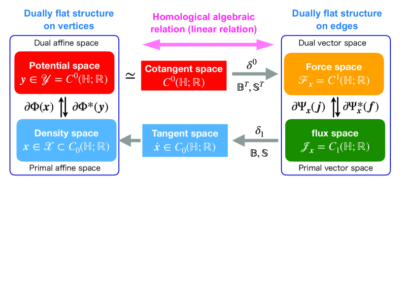
Figure 1: Diagrammatic illustration of the doubly dual flat structure established on the vertex affine spaces (left) and the edge spaces (right), which are topologically related via the underlying graph or hypergraph.

From the viewpoint of homological algebra, the structure we work on is a modification of the chain and cochain complexes of graphs or hypergraphs, which replace the usual inner product duality[73] on each pair of chains and cochains with Legendre duality. Moreover, the dually flat space built on the flux space is linked to a finite-dimensional version of Orlicz spaces[74], which have been employed for constructing infinite-dimensional information geometry[72]. From the nice properties of the doubly dual flat structures, we can obtain information-geometric extensions of the Helmholtz-Hodge-Kodaira (HHK) decomposition (Thm. 1), the Otto calculus (Thm. 2), and its induction to cycle spaces(Thm. 3).

Our construction of an information geometry for dynamics is heavily based on the idea of using Legendre duality for the force and flux relation, proposed in the recent work of large deviations theory and the macroscopic fluctuation theorem for MJP and CRN led by A.Mieleke, R.I.A.Petterson, M.A.Peletier, D.R.M. Renger, J.Zimmer, and others[75, 76, 77, 78, 79, 80, 81, 82]. We clarified its information-geometric aspects in the context of CRN and thermodynamics in our previous work[83]. We also concurrently elucidated the intimate link of equilibrium chemical thermodynamics and information geometry on the density state space [84, 85, 86]. In light of those, the contribution of this work is three-fold. First, we integrate these results in terms of information geometry, which clarifies the underlying geometric nature of the problem, provides transparent interpretations for known results, and leads to new information geometric results and insights (Thm. 1–Thm. 3); Second, this structure substantially extends the applicability of information geometry to a wide variety of dynamical problems; Lastly, the structure links information geometry to algebraic graph theory, discrete calculus, and homological algebra, which were not fully appreciated yet but provides a versatile way to consider the topology of the base manifold in information geometry.

I.5 Organization of this paper

This work is organized as follows: In Sec. II, we introduce a range of models of dynamics on graphs and hypergraphs. In Sec. III, we outline the homological algebra of graphs and hypergraphs. In Sec. IV, we abstractly introduce the doubly dual flat structures on the density and flux spaces and define the generalized flow associated with these structures. In Sec. V, we clarify that the introduced structures include a wide class of dynamics on graph and hypergraph. In Sec. VI and Sec. VII, we further define information-geometric objects and quantities, which naturally appear from this setup and play an integral role in the subsequent analysis of dynamics. In Sec. VIII and Sec. IX, we derive several results for equilibrium and nonequilibrium flows, respectively. Finally, we provide a summary and prospects of our work in Sec. X. The notations and symbols are listed in the appendix.

II Classes of models for density dynamics on graph and hypergraph

In this work, we focus on linear and nonlinear dynamics defined on graphs[87] and hypergraphs[88].

The linear dynamics of densities on graphs (LDG) includes Markov jump processes (MJP)[89], monomolecular chemical reaction networks[90], and others[87]. We consider an extension of LDG to hypergraphs and nonlinear dynamics, common instances of which are chemical reaction networks (CRN) with the law of mass action (LMA) kinetics [8] and polynomial dynamical systems (PDS)[91]. Because the extension we deal with in this work is a subclass of nonlinear dynamical systems on hypergraphs, we use CRN to designate this subclass.

In the following subsections, LDG and CRN are introduced using the language of algebraic graph theory[92, 87]. Then, we also give a brief and formal introduction of the Fokker-Planck equation (FPE)[3], a linear dynamics of probability densities defined in Euclidean space. We use the FPE throughout this paper only to contrast our results with the previous ones obtained for the FPE.

II.1 Reversible Linear Dynamics of Densities on Graphs

Definition 1 (Edge-weighted finite graph $\mathbb{G}_{\bm{k}^{\pm}}$).

A finite graph $\mathbb{G}:=(\{\mathbb{v}_{i}\},\{\mathbb{e}_{e}\},\mathbb{B})$ consists of $N_{\mathbb{v}}\in\mathbb{Z}_{>0}$ vertices, $\{\mathbb{v}_{i}\}_{i\in[1,N_{\mathbb{v}}]}$, and $N_{\mathbb{e}}\in\mathbb{Z}_{>0}$ oriented edges, $\{\mathbb{e}_{e}\}_{e\in[1,N_{\mathbb{e}}]}$, each of which connects two different vertices (Fig. 2 (a)). The incidence relation is represented by the incidence matrix $\mathbb{B}\in\{0,\pm 1\}^{N_{\mathbb{v}}\times N_{\mathbb{e}}}$ where, for $\mathbb{B}=(b_{i,e})$,

$$b_{i,e} :=+1 \mbox{if $\mathbb{v}_{i}$ is the head of edge $\mathbb{e}_{e}$},$$

$$b_{i,e} :=-1 \mbox{if $\mathbb{v}_{i}$ is the tail of edge $\mathbb{e}_{e}$},$$

$$b_{i,e} :=0 \mbox{otherwise}.$$

An edge-weighted finite graph $\mathbb{G}_{\bm{k}^{\pm}}:=(\{\mathbb{v}_{i}\},\{\mathbb{e}_{e}\},\mathbb{B},\{k_{e}^{\pm}\})$ has two positive weighting parameters $k_{e}^{\pm}=(k_{e}^{+},k_{e}^{-})\in\mathbb{R}_{>0}$ for each edge $\mathbb{e}_{e}$. Parameters $k_{e}^{+}$ and $k_{e}^{-}$ are denoted as forward and reverse rates or weights of edge $\mathbb{e}_{e}$, respectively.

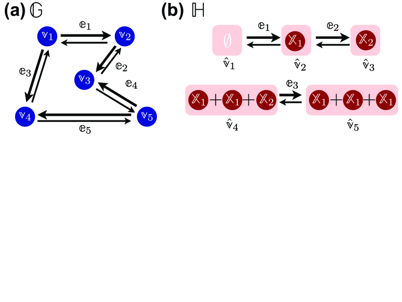
Figure 2: Schematic diagrams of the reversible finite graph $\mathbb{G}$ (a) and CRN-hypergraph $\mathbb{H}$ (b). Each pair of thick and thin arrows represents the pair of forward and reverse orientations of the corresponding edge. The CRN-hypergraph $\mathbb{H}$ in (b) corresponds to the simplified Brusselator reaction. The hypervertex $\hat{\mathbb{v}}_{1}$ contains no vertices.

A reversible linear dynamics (rLDG) on graphs is defined on the edge-weighted finite graph $\mathbb{G}_{\bm{k}^{\pm}}$:

Definition 2 (Reversible linear dynamics of density on graph $\mathbb{G}_{\bm{k}^{\pm}}$).

The reversible linear dynamics of the non-negative density $\bm{x}(t)=(x_{1}(t),\cdots,x_{N_{\mathbb{v}}}(t))^{T}\in\mathbb{R}_{\geq 0}^{N_{\mathbb{v}}}$ on $\mathbb{G}_{\bm{k}^{\pm}}$ is defined by the continuity equation

$$\dot{\bm{x}} =-\mathbb{B}\bm{j}(\bm{x})=-\mathbb{B}[\bm{j}^{+}(\bm{x})-\bm{j}^{-}(\bm{x})],$$ (2)

and linear forward and reverse one-way fluxes $\bm{j}^{\pm}(\bm{x})=(j^{\pm}_{1}(\bm{x}),\cdots,j^{\pm}_{N_{\mathbb{e}}}(\bm{x}))^{T}\in\mathbb{R}^{N_{\mathbb{e}}}_{\geq 0}$ with the following specific functional form:

$$\bm{j}^{\pm}(\bm{x}) =\bm{k}^{\pm}\circ(\mathbb{B}^{\pm})^{T}\bm{x},$$ (3)

where $\bm{j}(\bm{x}):=\bm{j}^{+}(\bm{x})-\bm{j}^{-}(\bm{x})$ is the total flux, the symbol $\circ$ denotes the component-wise product of two vectors, and $\mathbb{B}^{+}$ and $\mathbb{B}^{-}$ are the head and tail incidence matrices defined respectively as $\mathbb{B}^{+}:=\max[\mathbb{B},0]$ and $\mathbb{B}^{-}:=\max[-\mathbb{B},0]$. The incidence matrix $\mathbb{B}$ in Eq. 2 is often regarded as the discrete divergence operator on a graph [73] and denoted also by $\mathrm{div}_{\mathbb{B}}=\mathbb{B}$ to emphasize this interpretation in this work.

Reversible Markov jump processes (rMJP) are a representative class of the rLDG describing random jumps of noninteracting particles on $\mathbb{G}_{\bm{k}^{\pm}}$. The weighting parameter $k_{e}^{+}$ is interpreted as the forward jump rate from the head of the oriented edge $\mathbb{e}_{e}$ to its tail, whereas $k_{e}^{-}$ is the reverse jump rate from the tail to the head of $\mathbb{e}_{e}$. For infinitely many such particles, we consider $p_{i}(t)\in[0,1]$, the fraction of particles on vertex $\mathbb{v}_{i}$ at time $t$, which is a non-negative density on vertices. Then, the forward and reverse one-way fluxes on the $e$th edge defined by Eq. 3 are represented as

$$j^{+}_{e}(\bm{p}) =k_{e}^{+}p_{\mathbb{v}^{+}_{e}}\in\mathbb{R}_{\geq 0}, j^{-}_{e}(\bm{p}) =k_{e}^{-}p_{\mathbb{v}^{-}_{e}}\in\mathbb{R}_{\geq 0},$$ (4)

where $\mathbb{v}^{+}_{e}$ and $\mathbb{v}^{-}_{e}$ are the head and tail vertices of edge $\mathbb{e}_{e}$. The linearity of $j^{\pm}_{e}(\bm{p})$ with respect to $\bm{p}$ comes from the independence of particles on the graph. Then, the continuity equation (Eq. 2) with the state vector $\bm{p}(t):=(p_{1}(t),\cdots,p_{N_{\mathbb{v}}}(t))^{T}\in\mathbb{R}^{N_{\mathbb{v}}}_{\geq 0}$ is reduced to the master equation: $\dot{\bm{p}}=-\mathbb{B}\bm{j}(\bm{p})$.

Definition 3 (Weighted asymmetric graph Laplacian[92, 93]).

For $\mathbb{G}_{\bm{k}^{\pm}}$, the corresponding weighted asymmetric graph Laplacian is defined by

$$\mathcal{L}_{\bm{\theta}}:=\mathbb{B}\left[\mathrm{diag}[\bm{k}^{+}](\mathbb{B}^{+})^{T}-\mathrm{diag}[\bm{k}^{-}](\mathbb{B}^{-})^{T}\right],$$ (5)

where $\bm{\theta}:=(\bm{k}^{+},\bm{k}^{-})$ and $\mathrm{diag}[\bm{k}^{+}]$ is the diagonal matrix whose diagonal elements are $\bm{k}^{+}$. Using $\mathcal{L}_{\bm{\theta}}$, Eq. 2 and Eq. 3 are represented as

$$\dot{\bm{x}} =-\mathbb{B}\bm{j}(\bm{x})=-\mathbb{B}\left[\mathrm{diag}[\bm{k}^{+}](\mathbb{B}^{+})^{T}-\mathrm{diag}[\bm{k}^{-}](\mathbb{B}^{-})^{T}\right]\bm{x}=-\mathcal{L}_{\bm{\theta}}\bm{x}.$$ (6)

The operator $\mathcal{L}_{\bm{\theta}}$ is reduced to the weighted symmetric graph Laplacian if $\bm{k}^{+}=\bm{k}^{-}$ and also to the conventional graph Laplacian if $\bm{k}^{+}=\bm{k}^{-}=\bm{1}$[92, 93]. Eq. 6 can also cover linear transport on graphs, linear electric circuits [94], consensus dynamics on graphs [95], and other linear dynamics on graphs [87, 96].

II.2 Chemical reaction network and polynomial dynamical systems on hypergraphs

Next, we introduce a class of nonlinear dynamics on hypergraphs, which includes the rLDG (Eq. 2 and Eq. 3) as a special case. The most common instance is deterministic chemical reaction networks (CRN) with the law of mass action (LMA) kinetics[45, 7, 97, 8], and this class is sometimes referred to as polynomial dynamical systems (PDS). Because the major part of the PDS theory has been developed for CRN, we use CRN to introduce and specify this class in this work.

Definition 4 (Reversible edge-weighted CRN hypergraph $\mathbb{H}_{\bm{k}^{\pm}}$).

The reversible CRN hypergraph $\mathbb{H}:=(\{\mathbb{X}_{i}\},\{\mathbb{e}_{e}\},{\mathchoice{\raisebox{0.0pt}{\scalebox{1.0}[-1.0]{$\displaystyle\mathbb{L}$}}}{\raisebox{0.0pt}{\scalebox{1.0}[-1.0]{$\textstyle\mathbb{L}$}}}{\raisebox{0.0pt}{\scalebox{1.0}[-1.0]{$\scriptstyle\mathbb{L}$}}}{\raisebox{0.0pt}{\scalebox{1.0}[-1.0]{$\scriptscriptstyle\mathbb{L}$}}}},\mathbb{B})$ consists of a finite number of vertices $\{\mathbb{X}_{i}\}_{i\in[1,N_{\mathbb{X}}]}$ and hyperedges $\{\mathbb{e}_{e}\}_{e\in[1,N_{\mathbb{e}}]}$ where $N_{\mathbb{X}},N_{\mathbb{e}}\in\mathbb{Z}_{>0}$ (Fig. 2 (b)). Each hyperedge $\mathbb{e}_{e}$ connects two different hypervertices $\hat{\mathbb{v}}^{+}_{e}$ and $\hat{\mathbb{v}}^{-}_{e}$ where $\hat{\mathbb{v}}^{+}_{e}\neq\hat{\mathbb{v}}^{-}_{e}$. The hypervertices are multisets of vertices $\{\mathbb{X}_{i}\}_{i\in[1,N_{\mathbb{X}}]}$, each of which is defined as $\hat{\mathbb{v}}_{\ell}=\sum_{i=1}^{N_{\mathbb{X}}}\gamma_{i,\ell}\mathbb{X}_{i}$ where $\gamma_{i,\ell}\in\mathbb{Z}_{\geq 0}$ is the number of the $i$th vertex included in the $\ell$th hypervertex. Thus, the nonnegative integer vector $\bm{\gamma}_{\ell}:=(\gamma_{1,\ell},\cdots,\gamma_{N_{\mathbb{X}},\ell})^{T}\in\mathbb{Z}_{\geq 0}^{N_{\mathbb{X}}}$ defines the $\ell$th hypervertex. Let $N_{\hat{\mathbb{v}}}\in\mathbb{Z}_{>0}$ be the total number of the hypervertices and ${\mathchoice{\raisebox{0.0pt}{\scalebox{1.0}[-1.0]{$\displaystyle\mathbb{L}$}}}{\raisebox{0.0pt}{\scalebox{1.0}[-1.0]{$\textstyle\mathbb{L}$}}}{\raisebox{0.0pt}{\scalebox{1.0}[-1.0]{$\scriptstyle\mathbb{L}$}}}{\raisebox{0.0pt}{\scalebox{1.0}[-1.0]{$\scriptscriptstyle\mathbb{L}$}}}}:=(\bm{\gamma}_{1},\cdots,\bm{\gamma}_{N_{\hat{\mathbb{v}}}})\in\mathbb{Z}_{\geq 0}^{N_{\mathbb{X}}\times N_{\hat{\mathbb{v}}}}$ be the hypervertex matrix. The matrix $\mathbb{B}\in\{0,\pm 1\}^{N_{\hat{\mathbb{v}}}\times N_{\mathbb{e}}}$ is the incidence matrix encoding the incidence relations among the hypervertices and the hyperedges. The hypergraph incidence matrix $\mathbb{S}\in\mathbb{Z}^{N_{\mathbb{X}}\times N_{\mathbb{e}}}$ is then defined as

$$\mathbb{S}:={\mathchoice{\raisebox{0.0pt}{\scalebox{1.0}[-1.0]{$\displaystyle\mathbb{L}$}}}{\raisebox{0.0pt}{\scalebox{1.0}[-1.0]{$\textstyle\mathbb{L}$}}}{\raisebox{0.0pt}{\scalebox{1.0}[-1.0]{$\scriptstyle\mathbb{L}$}}}{\raisebox{0.0pt}{\scalebox{1.0}[-1.0]{$\scriptscriptstyle\mathbb{L}$}}}}\mathbb{B}.$$ (7)

If ${\mathchoice{\raisebox{0.0pt}{\scalebox{1.0}[-1.0]{$\displaystyle\mathbb{L}$}}}{\raisebox{0.0pt}{\scalebox{1.0}[-1.0]{$\textstyle\mathbb{L}$}}}{\raisebox{0.0pt}{\scalebox{1.0}[-1.0]{$\scriptstyle\mathbb{L}$}}}{\raisebox{0.0pt}{\scalebox{1.0}[-1.0]{$\scriptscriptstyle\mathbb{L}$}}}}=I$ where $I$ is the identity matrix, then $\mathbb{H}=(\{\mathbb{X}_{i}\}_{i\in[1,N_{\mathbb{X}}]},\{\mathbb{e}_{e}\}_{e\in[1,N_{\mathbb{e}}]},{\mathchoice{\raisebox{0.0pt}{\scalebox{1.0}[-1.0]{$\displaystyle\mathbb{L}$}}}{\raisebox{0.0pt}{\scalebox{1.0}[-1.0]{$\textstyle\mathbb{L}$}}}{\raisebox{0.0pt}{\scalebox{1.0}[-1.0]{$\scriptstyle\mathbb{L}$}}}{\raisebox{0.0pt}{\scalebox{1.0}[-1.0]{$\scriptscriptstyle\mathbb{L}$}}}},\mathbb{B})$ is reduced to $\mathbb{G}=(\{\mathbb{v}_{\ell}\}_{\ell\in[1,N_{\mathbb{X}}]},\{\mathbb{e}_{e}\}_{e\in[1,N_{\mathbb{e}}]},\mathbb{B})$ where $\mathbb{v}_{\ell}=\mathbb{X}_{\ell}$. An edge-weighted CRN hypergraph $\mathbb{H}_{\bm{k}^{\pm}}:=(\{\mathbb{X}_{i}\},\{\mathbb{e}_{e}\},{\mathchoice{\raisebox{0.0pt}{\scalebox{1.0}[-1.0]{$\displaystyle\mathbb{L}$}}}{\raisebox{0.0pt}{\scalebox{1.0}[-1.0]{$\textstyle\mathbb{L}$}}}{\raisebox{0.0pt}{\scalebox{1.0}[-1.0]{$\scriptstyle\mathbb{L}$}}}{\raisebox{0.0pt}{\scalebox{1.0}[-1.0]{$\scriptscriptstyle\mathbb{L}$}}}},\mathbb{B},\{k_{e}^{\pm}\})$ has forward and reverse rates $k_{e}^{\pm}>0$ as weights of edge $\mathbb{e}_{e}$.

In the context of CRN theory, the vertices $\{\mathbb{X}_{i}\}$ correspond to the molecular species involved in a CRN, and each hyperedge $\mathbb{e}_{e}$ represents a pair of forward and reverse reactions:

$$\gamma_{1,e}^{+}\mathbb{X}_{1}+\cdots+\gamma_{N_{\mathbb{X}},e}^{+}\mathbb{X}_{N_{\mathbb{X}}}\xrightleftharpoons{}\gamma^{-}_{1,e}\mathbb{X}_{1}+\cdots+\gamma^{-}_{N_{\mathbb{X}},e}\mathbb{X}_{N_{\mathbb{X}}},$$ (8)

where the forward and reverse reactions are from left to right and from right to left, respectively. Head and tail hypervertices $\hat{\mathbb{v}}_{e}^{+}:=(\gamma^{+}_{1,e}\mathbb{X}_{1}+\cdots+\gamma^{+}_{N_{\mathbb{X}},e}\mathbb{X}_{N_{\mathbb{X}}})$ and $\hat{\mathbb{v}}_{e}^{-}:=(\gamma^{-}_{1,e}\mathbb{X}_{1}+\cdots+\gamma^{-}_{N_{\mathbb{X}},e}\mathbb{X}_{N_{\mathbb{X}}})$ in Eq. 8 are the sets of reactants and products of the $e$th forward reaction, respectively. More specifically, $\gamma^{+}_{i,e}\in\mathbb{Z}_{\geq 0}$ and $\gamma^{-}_{i,e}\in\mathbb{Z}_{\geq 0}$ are the numbers of the molecule $\mathbb{X}_{i}$ involved as the reactants and products of the $e$th forward reaction, respectively. For the reverse reaction, $\hat{\mathbb{v}}_{e}^{-}$ and $\hat{\mathbb{v}}_{e}^{+}$ are the reactants and products. Some head and tail hypervertices are overlapping among different reactions (hyperedges) as in Fig. 2 (b). As a result, $\{\hat{\mathbb{v}}_{\ell}\}_{\ell\in N_{\hat{\mathbb{v}}}}$ is the union of the head and tail hypervertices, $\{\hat{\mathbb{v}}_{\ell}\}_{\ell\in N_{\hat{\mathbb{v}}}}=\bigcup_{e\in N_{\mathbb{e}}}\{\hat{\mathbb{v}}_{e}^{+},\hat{\mathbb{v}}_{e}^{-}\}$.

The hypervertices are called complexes in CRN theory [8]. From $\{\gamma^{+}_{i,e}\}$ and $\{\gamma^{-}_{i,e}\}$, we can define

$$\bm{s}_{e}:=(\gamma^{+}_{1,e}-\gamma^{-}_{1,e},\cdots,\gamma^{+}_{N_{\mathbb{X}},e}-\gamma^{-}_{N_{\mathbb{X}},e})^{T}\in\mathbb{Z}^{N_{\mathbb{X}}},$$ (9)

where $\mp\bm{s}_{e}$ specify the change in the number of molecules induced when the $e$th forward or reverse reaction occurs just once, respectively. The hypergraph incidence matrix $\mathbb{S}$ defined in Eq. 7 is represented as $\mathbb{S}=(\bm{s}_{1},\cdots,\bm{s}_{N_{\mathbb{e}}})\in\mathbb{Z}^{N_{\mathbb{X}}\times N_{\mathbb{e}}}$. In chemistry, the negative of $\bm{s}_{e}$ and $\mathbb{S}$, i.e., $-\bm{s}_{e}$ and $-\mathbb{S}$, are called the stoichiometric vector and matrix, respectively[8].

Remark 1.

To define a reversible CRN hypergraph, the hypergraph matrix $\mathbb{S}$ is not sufficient. If the head and tail hypervertices of a hyperedge contain the same vertex (molecule), the corresponding element in $\mathbb{S}$ of such a shared vertex becomes $0$ by canceling out. Thus, the existence of shared vertices (molecules) is invisible in $\mathbb{S}$, and the pair $({\mathchoice{\raisebox{0.0pt}{\scalebox{1.0}[-1.0]{$\displaystyle\mathbb{L}$}}}{\raisebox{0.0pt}{\scalebox{1.0}[-1.0]{$\textstyle\mathbb{L}$}}}{\raisebox{0.0pt}{\scalebox{1.0}[-1.0]{$\scriptstyle\mathbb{L}$}}}{\raisebox{0.0pt}{\scalebox{1.0}[-1.0]{$\scriptscriptstyle\mathbb{L}$}}}},\mathbb{B})$ is required to define $\mathbb{H}$. Such shared molecules are called catalysts in CRN.

For a CRN hypergraph, the continuity equation for CRN is defined:

Definition 5 (CRN continuity equation).

Let a vector of nonnegative densities $\bm{x}=(x_{1},\cdots,x_{N_{\mathbb{X}}})^{T}\in\mathbb{R}_{\geq 0}^{N_{\mathbb{X}}}$ represents the concentration of molecules $\{\mathbb{X}_{i}\}$. The CRN continuity equation is defined as

$$\dot{\bm{x}}=-\mathbb{S}\bm{j}(\bm{x})=-\mathrm{div}_{\mathbb{S}}\bm{j}(\bm{x}),$$ (10)

where $j_{e}^{+}(\bm{x})\in\mathbb{R}_{\geq 0}$ and $j_{e}^{-}(\bm{x})\in\mathbb{R}_{\geq 0}$ are the one-way fluxes of the $e$th forward and reverse reactions, $\bm{j}^{\pm}(\bm{x}):=(j_{1}^{\pm}(\bm{x}),\cdots,j_{N_{\mathbb{e}}}^{\pm}(\bm{x}))^{T}\in\mathbb{R}_{\geq 0}^{N_{\mathbb{e}}}$ are their vector representations, and $\bm{j}(\bm{x}):=\bm{j}^{+}(\bm{x})-\bm{j}^{-}(\bm{x})\in\mathbb{R}^{N_{\mathbb{e}}}$ is the total reaction flux[7, 97, 8]. The hypergraph divergence operator $\mathrm{div}_{\mathbb{S}}:=\mathbb{S}$ is defined accordingly.

To define the dynamics of a CRN, the functional form of $j_{e}^{\pm}(\bm{x})$ is required. Before introducing specific forms, we define two important properties of the fluxes and also other functions defined on edges:

Definition 6 (Consistency of fluxes $\bm{j}^{\pm}(\bm{x})$ with hypergraph $\mathbb{H}$).

One-way fluxes $\bm{j}^{\pm}(\bm{x})$ are consistent with the hypergraph $\mathbb{H}$ if, for all $e\in[1,N_{\mathbb{e}}]$, $j^{\pm}_{e}(\bm{x})$ becomes $0$ when $x_{i}=0$ where $\mathbb{X}_{i}$ is any reactant of $j^{\pm}_{e}(\bm{x})$, respectively. In other words, $j^{\pm}_{e}(\bm{x})$ satisfies $\gamma_{i,e}^{\pm}j_{e}^{\pm}(\bm{x})=0$ if $x_{i}=0$ for any $i\in[1,N_{\mathbb{X}}]$.

Definition 7 (Locality of function on edges over $\mathbb{H}$).

A vector function $\bm{g}(\bm{x})\in\mathbb{R}^{N_{\mathbb{e}}}$ defined on edges is local on $\mathbb{H}$ if, for all $e\in[1,N_{\mathbb{e}}]$, $g_{e}(\bm{x})$ is a function only of the elements of $\bm{x}$ incident to the edge $\mathbb{e}_{e}$ on $\mathbb{H}$, i.e., $g_{e}(\bm{x})=g_{e}(\bar{\gamma}_{1,e}^{+}x_{1},\cdots,\bar{\gamma}_{N_{\mathbb{X}},e}^{+}x_{N_{\mathbb{X}}},\bar{\gamma}_{1,e}^{-}x_{1},\cdots,\bar{\gamma}_{N_{\mathbb{X}},e}^{-}x_{N_{\mathbb{X}}})$ where $\bar{\gamma}_{i,e}^{\pm}:=\min[1,\gamma_{i,e}^{\pm}]\in\{0,1\}$.

The consistency condition is indispensable to prohibit a reaction that can decrease $x_{i}$ from occurring when $x_{i}=0$. For $\bm{j}^{\pm}(\bm{x})$, the locality means that the fluxes of the $e$th reaction depend only on the concentrations of their reactants and products. The local flux is determined solely by the information stored on the vertices incident to the edge and plays a crucial role when we regard the structure introduced in this work as an extension of differential forms on continuous manifolds to graphs and hypergraphs. When we work on specific forms of fluxes in this work, we consider only local fluxes consistent with the given hypergraph $\mathbb{H}$.

In chemistry, we have a variety of candidates for the functional form of flux, e.g., the Michaelis-Menten function, Hill’s function, and others[7, 98]. Among others, the LMA kinetics is the most basic and well-established one.

Definition 8 (Waage-Guldberg’s law of mass action kinetics (LMA kinetics)).

A CRN follows the LMA kinetics if, for all $e\in[1,N_{\mathbb{e}}]$, the $e$th forward and reverse reaction fluxes are represented as

$$j^{\pm}_{e}(\bm{x})=k^{\pm}_{e}\prod_{j=1}^{N_{\mathbb{X}}}x_{j}^{\gamma^{\pm}_{j,e}}=k^{\pm}_{e}\sum_{\ell=1}^{N_{\hat{\mathbb{v}}}}b_{\ell,e}^{\pm}\prod_{j=1}^{N_{\mathbb{X}}}x_{j}^{\gamma_{j,\ell}},$$ (11)

where $k_{e}^{+}\in\mathbb{R}_{>0}$ and $k_{e}^{-}\in\mathbb{R}_{>0}$ are the reaction rate constants of the $e$th forward and reverse reactions, respectively. The fluxes under LMA kinetics can be compactly represented as

$$\bm{j}^{\pm}_{\mathrm{MA}}(\bm{x})=\bm{k}^{\pm}\circ(\mathbb{B}^{\pm})^{T}\bm{x}^{{\mathchoice{\raisebox{0.0pt}{\scalebox{1.0}[-1.0]{$\displaystyle\mathbb{L}$}}}{\raisebox{0.0pt}{\scalebox{1.0}[-1.0]{$\textstyle\mathbb{L}$}}}{\raisebox{0.0pt}{\scalebox{1.0}[-1.0]{$\scriptstyle\mathbb{L}$}}}{\raisebox{0.0pt}{\scalebox{1.0}[-1.0]{$\scriptscriptstyle\mathbb{L}$}}}}^{T}},$$ (12)

where $\bm{x}^{\bm{\gamma}}:=\prod_{j=1}^{N_{\mathbb{X}}}x_{j}^{\gamma_{j}}\in\mathbb{R}_{\geq 0}$ and $\bm{x}^{{\mathchoice{\raisebox{0.0pt}{\scalebox{1.0}[-1.0]{$\displaystyle\mathbb{L}$}}}{\raisebox{0.0pt}{\scalebox{1.0}[-1.0]{$\textstyle\mathbb{L}$}}}{\raisebox{0.0pt}{\scalebox{1.0}[-1.0]{$\scriptstyle\mathbb{L}$}}}{\raisebox{0.0pt}{\scalebox{1.0}[-1.0]{$\scriptscriptstyle\mathbb{L}$}}}}^{T}}:=(\bm{x}^{\bm{\gamma}_{1}},\cdots,\bm{x}^{\bm{\gamma}_{N_{\hat{\mathbb{v}}}}})^{T}\in\mathbb{R}_{\geq 0}^{N_{\hat{\mathbb{v}}}}$. We use the subscript $\mathrm{MA}$ as in $\bm{j}^{\pm}_{\mathrm{MA}}(\bm{x})$ to discriminate this specific form of the fluxes from others. We can easily observe that $\bm{j}^{\pm}_{\mathrm{MA}}(\bm{x})$ is consistent and local with respect to $\mathbb{H}$. Furthermore, $\bm{j}^{\pm}_{\mathrm{MA}}(\bm{x})$ is specified by the edge-weighted CRN hypergraph $\mathbb{H}_{\bm{k}^{\pm}}:=(\{\mathbb{X}_{i}\},\{\mathbb{e}_{e}\},{\mathchoice{\raisebox{0.0pt}{\scalebox{1.0}[-1.0]{$\displaystyle\mathbb{L}$}}}{\raisebox{0.0pt}{\scalebox{1.0}[-1.0]{$\textstyle\mathbb{L}$}}}{\raisebox{0.0pt}{\scalebox{1.0}[-1.0]{$\scriptstyle\mathbb{L}$}}}{\raisebox{0.0pt}{\scalebox{1.0}[-1.0]{$\scriptscriptstyle\mathbb{L}$}}}},\mathbb{B},\{k_{e}^{\pm}\})$.

Remark 2 (Algebraic aspect of LMA kinetics).

Because $\bm{x}^{{\mathchoice{\raisebox{0.0pt}{\scalebox{1.0}[-1.0]{$\displaystyle\mathbb{L}$}}}{\raisebox{0.0pt}{\scalebox{1.0}[-1.0]{$\textstyle\mathbb{L}$}}}{\raisebox{0.0pt}{\scalebox{1.0}[-1.0]{$\scriptstyle\mathbb{L}$}}}{\raisebox{0.0pt}{\scalebox{1.0}[-1.0]{$\scriptscriptstyle\mathbb{L}$}}}}^{T}}$ is a vector of monomials of $\bm{x}$, each one-way flux, $j^{\pm}_{e}(\bm{x})$, is a monomial of $\bm{x}$ under Eq. 12 and thus the total flux $j_{e}(\bm{x})=j^{+}_{e}(\bm{x})-j^{-}_{e}(\bm{x})$ is a binomial. This fact links the real algebraic geometry of the toric varieties[99, 100] to CRN[101, 102] as it does in algebraic statistics[103, 104].

Remark 3 (Extended LMA kinetics).

While we mainly work on the normal LMA kinetics, we can extend it. The extended LMA kinetics defined on $\mathbb{H}$ is defined as

$$\bm{j}^{\pm}_{\mathrm{eMA}}(\bm{x})=\bm{k}^{\pm}\circ\bm{g}(\bm{x})\circ(\mathbb{B}^{\pm})^{T}\bm{x}^{{\mathchoice{\raisebox{0.0pt}{\scalebox{1.0}[-1.0]{$\displaystyle\mathbb{L}$}}}{\raisebox{0.0pt}{\scalebox{1.0}[-1.0]{$\textstyle\mathbb{L}$}}}{\raisebox{0.0pt}{\scalebox{1.0}[-1.0]{$\scriptstyle\mathbb{L}$}}}{\raisebox{0.0pt}{\scalebox{1.0}[-1.0]{$\scriptscriptstyle\mathbb{L}$}}}}^{T}},$$ (13)

where $\bm{g}(\bm{x})\in\mathbb{R}_{>0}^{N_{\mathbb{e}}}$ and is local with respect to $\mathbb{H}$. An example of the extended LMA kinetics is reversible Michaelis-Menten kinetics[106].

By combining the continuity equation (Eq. 10) and the LMA kinetics (Eq. 12), we have the following chemical rate equation:

$$\dot{\bm{x}} =-\mathbb{S}\bm{j}_{\mathrm{MA}}(\bm{x})=-{\mathchoice{\raisebox{0.0pt}{\scalebox{1.0}[-1.0]{$\displaystyle\mathbb{L}$}}}{\raisebox{0.0pt}{\scalebox{1.0}[-1.0]{$\textstyle\mathbb{L}$}}}{\raisebox{0.0pt}{\scalebox{1.0}[-1.0]{$\scriptstyle\mathbb{L}$}}}{\raisebox{0.0pt}{\scalebox{1.0}[-1.0]{$\scriptscriptstyle\mathbb{L}$}}}}\mathbb{B}\left[\mathrm{diag}[\bm{k}^{+}](\mathbb{B}^{+})^{T}-\mathrm{diag}[\bm{k}^{-}](\mathbb{B}^{-})^{T}\right]\bm{x}^{{\mathchoice{\raisebox{0.0pt}{\scalebox{1.0}[-1.0]{$\displaystyle\mathbb{L}$}}}{\raisebox{0.0pt}{\scalebox{1.0}[-1.0]{$\textstyle\mathbb{L}$}}}{\raisebox{0.0pt}{\scalebox{1.0}[-1.0]{$\scriptstyle\mathbb{L}$}}}{\raisebox{0.0pt}{\scalebox{1.0}[-1.0]{$\scriptscriptstyle\mathbb{L}$}}}}^{T}}=-{\mathchoice{\raisebox{0.0pt}{\scalebox{1.0}[-1.0]{$\displaystyle\mathbb{L}$}}}{\raisebox{0.0pt}{\scalebox{1.0}[-1.0]{$\textstyle\mathbb{L}$}}}{\raisebox{0.0pt}{\scalebox{1.0}[-1.0]{$\scriptstyle\mathbb{L}$}}}{\raisebox{0.0pt}{\scalebox{1.0}[-1.0]{$\scriptscriptstyle\mathbb{L}$}}}}\mathcal{L}_{\bm{\theta}}\bm{x}^{{\mathchoice{\raisebox{0.0pt}{\scalebox{1.0}[-1.0]{$\displaystyle\mathbb{L}$}}}{\raisebox{0.0pt}{\scalebox{1.0}[-1.0]{$\textstyle\mathbb{L}$}}}{\raisebox{0.0pt}{\scalebox{1.0}[-1.0]{$\scriptstyle\mathbb{L}$}}}{\raisebox{0.0pt}{\scalebox{1.0}[-1.0]{$\scriptscriptstyle\mathbb{L}$}}}}^{T}},$$ (14)

where $\mathcal{L}_{\bm{\theta}}$ is the weighted asymmetric graph Laplacian defined as in Eq. 5. Now, we can see that CRN contains rLDG (Eq. 6) as a special case if ${\mathchoice{\raisebox{0.0pt}{\scalebox{1.0}[-1.0]{$\displaystyle\mathbb{L}$}}}{\raisebox{0.0pt}{\scalebox{1.0}[-1.0]{$\textstyle\mathbb{L}$}}}{\raisebox{0.0pt}{\scalebox{1.0}[-1.0]{$\scriptstyle\mathbb{L}$}}}{\raisebox{0.0pt}{\scalebox{1.0}[-1.0]{$\scriptscriptstyle\mathbb{L}$}}}}=I$. Owing to this inclusion relation, CRN with LMA kinetics is a mathematically sound generalization of rLDG. Because LDG has been used in various fields of social science, network science, machine learning, and so on, CRN theory is potentially important for extending the results there.

Example 1 (Simplified Brusselator CRN[8, 107]).

The Brusselator is a representative CRN, which can generate non-trivial dynamic behaviors such as oscillations. We use a reversible CRN version of the simplified Brusselator[8, 107], whose CRN-hypergraph depicted in Fig. 2 (b) has the following structural information:

$$\mathbb{L} =\bordermatrix{&\hat{\mathbb{v}}_{1}&\hat{\mathbb{v}}_{2}&\hat{\mathbb{v}}_{3}&\hat{\mathbb{v}}_{4}&\hat{\mathbb{v}}_{5}\cr\mathbb{X}_{1}&0&1&0&2&3\cr\mathbb{X}_{2}&0&0&1&1&0\cr}, \mathbb{B} =\bordermatrix{&\mathbb{e}_{1}&\mathbb{e}_{2}&\mathbb{e}_{3}\cr\hat{\mathbb{v}}_{1}&+1&0&0\cr\hat{\mathbb{v}}_{2}&-1&+1&0\cr\hat{\mathbb{v}}_{3}&0&-1&0\cr\hat{\mathbb{v}}_{4}&0&0&+1\cr\hat{\mathbb{v}}_{5}&0&0&-1\cr}, \mathbb{S} =\bordermatrix{&\mathbb{e}_{1}&\mathbb{e}_{2}&\mathbb{e}_{3}\cr\mathbb{X}_{1}&-1&+1&-1\cr\mathbb{X}_{2}&0&-1&+1\cr}$$ (15)

,

The rate equation (Eq. 14) can be represented as

$$\frac{\mathrm{d}}{\mathrm{d}t}\begin{pmatrix}x_{1}\\ x_{2}\end{pmatrix}=-\overbrace{\begin{pmatrix}-1&+1&-1\\ 0&-1&+1\end{pmatrix}}^{\mathbb{S}}\left[\overbrace{\begin{pmatrix}k_{1}^{+}\\ k_{2}^{+}x_{1}\\ k_{3}^{+}x_{1}^{2}x_{2}\end{pmatrix}}^{\bm{j}^{+}(\bm{x})}-\overbrace{\begin{pmatrix}k_{1}^{-}x_{1}\\ k_{2}^{-}x_{2}\\ k_{3}^{-}x_{1}^{3}\end{pmatrix}}^{\bm{j}^{-}(\bm{x})}\right].$$ (16)

II.3 Fokker Planck Equations

While our main focus is the dynamics on graphs and hypergraphs, we use FPE as a representative class of density dynamics on a continuous Euclidean space. Specifically, we use FPE only to demonstrate the relation of our results with previous ones obtained for FPE in various contexts. Because FPE is infinite-dimensional, we treat it here only formally.

Let $\bm{r}\in\mathbb{R}^{d}$ be a vector in a $d$ dimensional Euclidean space. We consider infinitely many noninteracting particles randomly walking in the space and describe the dynamics by a probability density $p_{t}(\bm{r})\in\mathbb{R}_{\geq 0}$ of the particles. The continuity equation for $p_{t}(\bm{r})$ is

$$\partial_{t}p_{t}(\bm{r}) =-\nabla\cdot\bm{j}_{\mathrm{FP}}[p_{t}(\bm{r})]$$ (17)

where $\bm{j}_{\mathrm{FP}}[p_{t}(\bm{r})]\in\mathbb{R}^{d}$ is the probability flux, $\nabla:=(\partial/\partial r_{1},\cdots,\partial/\partial r_{d})^{T}$ is the gradient operator on the Euclidean space, and $(\nabla\cdot):\nabla\cdot\bm{F}(\bm{r}):=\sum_{i=1}^{d}\partial F_{i}(\bm{r})/\partial r_{i}\in\mathbb{R}$ is the divergence. The flux of the FPE is defined as

$$\bm{j}_{\mathrm{FP}}[p(\bm{r})] =\left[\bm{F}(\bm{r})p(\bm{r})-D_{0}\nabla p(\bm{r})\right],$$ (18)

where $\bm{F}(\bm{r})\in\mathbb{R}^{d}$ is the drift force, and $D_{0}\in\mathbb{R}_{>0}$ is the diffusion constant.

III Discrete Calculus and Homological Algebra of Graphs and Hypergraphs

The algebraic and topological structure of the dynamics on graphs and hypergraphs can be explicitly and abstractly treated using the language of discrete calculus and homological algebra. The discrete version of the gradient and divergence mentioned in Sec. II is also characterized. In this section, we briefly introduce the chain and cochain complexes defined for a finite graph or a hypergraph and discrete calculus[92, 73, 108, 109]. We first introduce the complexes for a graph $\mathbb{G}$ and then extend them to a hypergraph $\mathbb{H}$ algebraically. It should be noted that the conventional discrete calculus (the discrete version of the theory for differential forms) presumes the Riemannian metric structure in the dual space of chains and cochains or that of cochains on primal and dual complexes [110, 111]. However, we are going to introduce Legendre duality instead. For this purpose, our introduction of chain and cochain complexes depends only on the topological (algebraic) information of the underlying graph and hypergraph[73] without specifying the metric information.

III.1 Chain and cochain complexes on graphs

The elements of a graph $\mathbb{G}$ are called cells in discrete calculus . A vertex and an edge are, respectively, called $0$-cell and $1$-cell, and the graph $\mathbb{G}$ is denoted as a cell-complex. For each type of the cells, we consider vectors (chains and cochains) defined on the cells. For $\mathbb{G}$, a $0$-chain with field $\mathbb{R}$ is an $N_{\mathbb{v}}$-tuple of real scalars, each of which is assigned to a vertex, i.e., a $0$ cell. Thus, a $0$-chain is a real vector defined on the vertices of $\mathbb{G}$ with the basis $\{\mathbb{v}_{i}\}$. This basis is called the standard basis. The vector space of real $0$-chains is called the vertex space here and denoted as $C_{0}(\mathbb{G})=\mathbb{R}^{N_{\mathbb{v}}}$[92]. The components of the vector $\bm{x}\in C_{0}(\mathbb{G})$ are given as $\bm{x}(\mathbb{v}_{i}):=x_{i}$. Similarly, a real $1$-chain is a real vector defined on the edges of $\mathbb{G}$. The real vector space of $1$-chains is called the edge space and denoted as $C_{1}(\mathbb{G})=\mathbb{R}^{N_{\mathbb{e}}}$. The standard basis is introduced by using edges $\{\mathbb{e}_{e}\}$, accordingly. A flux $\bm{j}$ is a $1$-chain: $\bm{j}(\mathbb{e}_{e}):=j_{e}$. The graph incidence matrix $\mathbb{B}$ induces the discrete differential $\delta_{1}:C_{1}(\mathbb{G})\to C_{0}(\mathbb{G})$ as $\delta_{1}\bm{j}:=\mathbb{B}\bm{j}$.

To obtain an exact sequence, we algebraically define the $(-1)$ and $2$ chains and the corresponding differentials $\delta_{0}$ and $\delta_{2}$. Let $C_{2}(\mathbb{G})=\mathbb{R}^{N_{\mathbb{z}}}$ where $N_{\mathbb{z}}=\mathrm{dim}[\mathrm{Ker}\mathbb{B}]$ and $\{\bm{v}_{i}\}_{i\in[1,N_{\mathbb{z}}]}$ is a set of complete basis of $\mathrm{Ker}\mathbb{B}$ where $\bm{v}_{i}\in\{0,+1,-1\}^{N_{\mathbb{e}}}$. In algebraic graph theory, $\mathrm{Ker}\mathbb{B}$ is called a cycle subspace[92, 112, 87]. For a graph $\mathbb{G}$, we can construct $\{\bm{v}_{i}\}_{i\in[1,N_{\mathbb{z}}]}$ by, for example, using the fundamental cycle basis of $\mathbb{G}$ obtained from a fixed spanning tree of $\mathbb{G}$[87]. Thus, $C_{2}(\mathbb{G})$ is the vector space defined on the cycles of $\mathbb{G}$ and isomorphic to the cycle subspace. We define a matrix, $\mathbb{V}:=(\bm{v}_{1},\cdots,\bm{v}_{N_{\mathbb{z}}})$, and the differential $\delta_{2}:C_{2}(\mathbb{G})\to C_{1}(\mathbb{G})$ as $\delta_{2}:=\mathbb{V}$. From the construction, $\mathbb{B}\mathbb{V}=\delta_{1}\delta_{2}=0$ and $\mathrm{Im}[\delta_{2}]=\mathrm{Ker}[\delta_{1}]$ hold. Similarly, let $C_{-1}(\mathbb{G})=\mathbb{R}^{N_{\mathbb{l}}}$ where $N_{\mathbb{l}}=\mathrm{dim}[\mathrm{Ker}\mathbb{B}^{T}]$ and $\{\bm{u}_{\ell}\}_{\ell\in[1,N_{\mathbb{l}}]}$ is a set of complete basis of $\mathrm{Ker}\mathbb{B}^{T}$ where $\bm{u}_{\ell}\in\{0,+1,-1\}^{N_{\mathbb{v}}}$. The subspace $\mathrm{Ker}\mathbb{B}^{T}$ is related to the connected components of $\mathbb{G}$ and $\bm{u}_{i}$ can be chosen such that $u_{i,\ell}=+1$ if the $i$th vertex is included in the $\ell$th connected component and $u_{i,\ell}=0$, otherwise. Thus, $C_{-1}(\mathbb{G})$ is the vector space on the connected components. From the matrix $\mathbb{U}:=(\bm{u}_{1},\cdots,\bm{u}_{N_{\mathbb{l}}})^{T}$, the differential $\delta_{0}:C_{0}(\mathbb{G})\to C_{-1}(\mathbb{G})$ is defined as $\delta_{0}:=\mathbb{U}$. From the construction, $\mathbb{U}\mathbb{B}=\delta_{0}\delta_{1}=0$ and $\mathrm{Im}[\delta_{1}]=\mathrm{Ker}[\delta_{0}]$ hold. Then, we obtain the exact chain sequence:

$$0\xleftarrow{}C_{-1}(\mathbb{G})\xleftarrow{\delta_{0}=\mathbb{U}}C_{0}(\mathbb{G})\xleftarrow{\delta_{1}=\mathbb{B}}C_{1}(\mathbb{G})\xleftarrow{\delta_{2}=\mathbb{V}}C_{2}(\mathbb{G})\xleftarrow{}0.$$ (19)

Because $C_{p}(\mathbb{G})$ is a vector space for each $p\in\{-1,0,1,2\}$, we can consider its dual vector space $C^{p}(\mathbb{G}):=C_{p}^{*}(\mathbb{G})$ consisting of the linear functions on $C_{p}(\mathbb{G})$. An element of $C^{p}(\mathbb{G})$ is called $p$-cochain. Let $\langle\cdot,\cdot\rangle:C_{p}(\mathbb{G})\times C^{p}(\mathbb{G})\to\mathbb{R}$ be the standard bilinear pairing of the $p$-chain and $p$-cochain defined with the standard basis. The transposes of $\mathbb{U}$, $\mathbb{B}$, and $\mathbb{V}$ induce the differentials between cochains as $\delta^{-1}:=\mathbb{U}^{T}:C^{-1}(\mathbb{G})\to C^{0}(\mathbb{G})$, $\delta^{0}:=\mathbb{B}^{T}:C^{0}(\mathbb{G})\to C^{1}(\mathbb{G})$, and $\delta^{1}:=\mathbb{V}^{T}:C^{1}(\mathbb{G})\to C^{2}(\mathbb{G})$. The differentials $\delta^{p}$ on cochains are the adjoints of the differentials $\delta_{p}$ on chains, which induce the exact cochain sequence:

$$0\xrightarrow{}C^{-1}(\mathbb{G})\xrightarrow{\delta^{-1}=\mathbb{U}^{T}}C^{0}(\mathbb{G})\xrightarrow{\delta^{0}=\mathbb{B}^{T}}C^{1}(\mathbb{G})\xrightarrow{\delta^{1}=\mathbb{V}^{T}}C^{2}(\mathbb{G})\xrightarrow{}0.$$ (20)

Note that the definition of chains, cochains, and differential operators are topological in the sense that we do not include any metric information.

III.2 Chain and cochain complexes on hypergraphs

The definitions of chain and cochain complexes introduced above are algebraically extended to hypergraphs $\mathbb{H}$ simply by replacing the graph incidence matrix $\mathbb{B}$ with the hypergraph incidence matrix $\mathbb{S}$.

Definition 9 (Exact chain and cochain sequences on a hypergraph).

The chain and cochain complexes on a hypergraph are defined by the following diagram:

$$0 \xrightarrow{} C^{-1}(\mathbb{H}) \xrightarrow{\delta^{-1}=\mathbb{U}^{T}} C^{0}(\mathbb{H}) \xrightarrow{\delta^{0}=\mathbb{S}^{T}} C^{1}(\mathbb{H}) \xrightarrow{\delta^{1}=\mathbb{V}^{T}} C^{2}(\mathbb{H}) \xrightarrow{} 0$$

$$0 \xleftarrow{} C_{-1}(\mathbb{H}) \xleftarrow{\delta_{0}=\mathbb{U}} C_{0}(\mathbb{H}) \xleftarrow{\delta_{1}=\mathbb{S}} C_{1}(\mathbb{H}) \xleftarrow{\delta_{2}=\mathbb{V}} C_{2}(\mathbb{H}) \xleftarrow{} 0$$ .

where $C^{-1}(\mathbb{H})\simeq C_{-1}(\mathbb{H})\simeq\mathbb{R}^{N_{\mathbb{l}}}$, $C^{0}(\mathbb{H})\simeq C_{0}(\mathbb{H})\simeq\mathbb{R}^{N_{\mathbb{X}}}$, $C^{1}(\mathbb{H})\simeq C_{1}(\mathbb{H})\simeq\mathbb{R}^{N_{\mathbb{e}}}$, and $C^{2}(\mathbb{H})\simeq C_{2}(\mathbb{H})\simeq\mathbb{R}^{N_{\mathbb{z}}}$.

The bases, $\mathbb{V}$ and $\mathbb{U}$, are obtained as integral bases, i.e., the components of $\mathbb{V}$ and $\mathbb{U}$ can be chosen from $\mathbb{Z}$ because $\mathbb{S}$ is an integer-valued matrix. As we will explain in Sec. VI and Sec. IX, the meaning of $C_{2}(\mathbb{H})$ can be retained as the space on generalized cycles. The meaning of $C_{-1}(\mathbb{H})$ becomes the space of conserved quantities under the dynamics (Eq. 10).

III.3 Discrete calculus on graphs and hypergraphs

The $p$-cochain and $p$-chain introduced above are an algebraic abstraction of the $p$-differential form and its Hodge dual on a differential manifold[73]. Accordingly, the discrete versions of gradient, divergence, and curl are associated with the differentials (exterior derivative).

Definition 10 (Discrete gradients, divergences, and curls).

The discrete gradient is defined as $\mathrm{grad}_{\mathbb{B}}:=\delta^{0}=\mathbb{B}^{T}$ for $\mathbb{G}$ and also as $\mathrm{grad}_{\mathbb{S}}:=\delta^{0}=\mathbb{S}^{T}$ for $\mathbb{H}$. The adjoints of the gradients are defined with the corresponding adjoint differentials: $\mathrm{grad}^{*}_{\mathbb{B}}:=\delta_{1}=\mathbb{B}$ and $\mathrm{grad}^{*}_{\mathbb{S}}:=\delta_{1}=\mathbb{S}$. They are called discrete divergences and denoted also as $\mathrm{div}_{\mathbb{B}}=\mathrm{grad}^{*}_{\mathbb{B}}$ and $\mathrm{div}_{\mathbb{S}}=\mathrm{grad}^{*}_{\mathbb{S}}$. The discrete curl and its adjoint are defined as $\mathrm{curl}_{\mathbb{V}}:=\delta^{1}=\mathbb{V}^{T}$ and $\mathrm{curl}^{*}_{\mathbb{V}}:=\delta_{2}=\mathbb{V}$, respectively.

III.4 Linear Graph Laplacian Dynamics and Metric structure in discrete calculus

In the theory of graph Laplacian, a metric matrix $M_{p}$ and its associated inner product are typically endowed for each $p$. To contrast it with the Legendre duality introduced later, we briefly outline it here. For an edge-weighted graph $\mathbb{G}_{\bm{k}^{\pm}}$ and for the case that $\bm{k}^{+}=\bm{k}^{-}=\bm{k}\in\mathbb{R}_{>0}^{N_{\mathbb{e}}}$, $M_{0}=I$ and $M_{1}=\mathrm{diag}[1/\bm{k}]$ are conventionally employed. With these metric matrices, the graph Laplacian introduced in Eq. 5 can be described as

$$\mathcal{L}_{\bm{k}}=\mathrm{div}_{\mathbb{B}}M^{1}\mathrm{grad}_{\mathbb{B}}M_{0}$$ (21)

where $M^{p}:=M_{p}^{-1}$. By including such metric information, the following pair of metric gradient and divergence is often used in graph theory and network theory: $\mathrm{grad}_{M}:=\sqrt{M^{1}}\mathbb{B}^{T}$ and $\mathrm{div}_{M}:=\mathbb{B}\sqrt{M^{1}}$ where $\sqrt{M^{1}}:=\mathrm{diag}[\sqrt{\bm{k}}]$. This symmetric graph Laplacian $\mathcal{L}_{\bm{k}}$ induces a linear dynamics of $\bm{x}\in\mathbb{R}^{N_{\mathbb{v}}}$ on graph via Eq. 6:

$$\dot{\bm{x}}=-\mathcal{L}_{\bm{k}}\bm{x}.$$ (22)

The eigenvalues and eigenvectors of $\mathcal{L}_{\bm{k}}$ enable us to obtain spectral information of the underlying graph[93]. Even for nonlinear dynamics on a hypergraph as in Eq. 14, the same symmetric Laplacian can provide some information when $\bm{k}^{+}=\bm{k}^{-}=\bm{k}$. We can also include other information in the metric matrices such as the degree of vertices[113]. Various normalizations of the graph Laplacian can be attributed to the choice of metrics.

However, such a choice of metric matrices ends up only with linear dynamics on $\mathbb{R}^{N_{\mathbb{v}}}$ and is relevant only when the weighting is symmetric: $\bm{k}^{+}=\bm{k}^{-}=\bm{k}$. In addition, it may not always capture important aspects of the density dynamics such as gradient flow properties and information-theoretic properties, because nonlinear terms such as $\ln\bm{p}$ appear in information-theoretic quantities. To extend the class of dynamics being covered and to enable the information-geometric characterization of dynamics, we have to generalize the conventional inner product structure by replacing it with the Legendre dual structure induced by convex functions.

IV Dually flat spaces on vertices and edges and generalized flow

In this section, we introduce two pairs of dually flat spaces (Fig. 1): one is associated with the vertex spaces, i.e., the dual spaces of $0$-chains and $0$-cochains. The other corresponds to the edge spaces, i.e., the dual spaces of $1$-chains and $1$-cochains. By combining them, the dynamics on graphs and hypergraphs are characterized as a generalized flow.

IV.1 Dually flat spaces on vertices and thermodynamic functions

We work on the density $\bm{x}$ and the vertex space for CRN because its reduction to rLDG is straightforward. For a probability vector $\bm{p}$, the introduction of dually flat spaces of $\bm{p}$ and $\ln\bm{p}$ is natural from the information-geometric viewpoint. In CRN, $\bm{x}$ is the vector of concentrations of molecular species. As we recently clarified[48, 102], the dually flat spaces, in this case, result from the Legendre duality between extensive and intensive variables in thermodynamics, which is also natural from the physical viewpoint.

Definition 11 (Density space (primal vertex affine space)).

The density space (also called primal affine vertex space) is the positive orthant $\mathcal{X}:=\mathbb{R}_{>0}^{N_{\mathbb{X}}}$ of a vector space $\mathbb{R}^{N_{\mathbb{X}}}$, which is isomorphic to $C_{0}(\mathbb{H})$: $\mathbb{R}^{N_{\mathbb{X}}}\simeq C_{0}(\mathbb{H})$ (Fig. 1, lower left).

Remark 4.

The density space $\mathcal{X}$ is defined as the positive orthant rather than as $\mathbb{R}_{\geq 0}^{N_{\mathbb{X}}}$. This excludes the cases where some elements of $\bm{x}$ become $0$. From the viewpoint of information geometry, this restriction is necessary to consider densities with the same support (all $\bm{x}$ in $\mathcal{X}$ should be equivalent in terms of absolute continuity of measures). From the viewpoint of dynamical systems, depending on the specific functional form of the flux $\bm{j}(\bm{x})$, the trajectory $\bm{x}(t)$ may not be restricted within $\mathcal{X}$. The property $\bm{x}(t)$ in $\mathcal{X}$ for $t\in[0,\infty]$ is known as persistence. Without going into this intricate problem, we simply assume that $\bm{x}(t)\in\mathcal{X}$ for $t\in[0,\infty]$. We call $\partial\mathcal{X}:=\mathbb{R}^{N_{\mathbb{X}}}_{\geq 0}\setminus\mathcal{X}$ the boundary of $\mathcal{X}$.

We define the dual of the density space by the Legendre transformation via the thermodynamic function:

Definition 12 (Primal thermodynamic function).

A strictly convex differentiable function $\Phi:\mathcal{X}\to\mathbb{R}$ is called the primal thermodynamic function if the following two conditions are satisfied: (1) the associated Legendre transformation

$$\partial\Phi:\mathcal{X} \to\mathbb{R}^{N_{\mathbb{X}}}$$ (23)

$$\bm{x} \longmapsto\bm{y}:=\partial_{\bm{x}}\Phi(\bm{x})=\left(\frac{\partial\Phi(\bm{x})}{\partial x_{1}},\cdots,\frac{\partial\Phi(\bm{x})}{\partial x_{N_{\mathbb{X}}}}\right)^{T}$$ (24)

has the image $\mathcal{Y}:=\left\{\bm{y}|\bm{y}=\partial\Phi(\bm{x}),\bm{x}\in\mathcal{X}\right\}$ being equal to $\mathbb{R}^{N_{\mathbb{X}}}$, i.e., $\mathcal{Y}=\mathbb{R}^{N_{\mathbb{X}}}$; (2) for any $\bm{x}_{in}\in\mathcal{X}$ and any point on the boundary $\bm{x}_{bd}\in\partial\mathcal{X}$,

$$\lim_{\lambda\to+0}\frac{\mathrm{d}\Phi(\bm{x}_{\lambda})}{\mathrm{d}\lambda}=-\infty$$ (25)

holds where $\bm{x}_{\lambda}:=\lambda\bm{x}_{in}+(1-\lambda)\bm{x}_{bd}$ for $\lambda\in[0,1]$.

Definition 13 (Potential space (dual affine vertex space) and dual thermodynamic function).

The potential (field) space $\mathcal{Y}=\mathbb{R}^{N_{\mathbb{X}}}$ (also called the dual affine vertex space) is an affine space dual to $\mathcal{X}$ with the associated vector space $C^{0}(\mathbb{H})$((Fig. 1, upper left)). The dual thermodynamic function $\Phi^{*}:\mathcal{Y}\to\mathbb{R}$ is the Legendre-Fenchel conjugate of the primal thermodynamic function:

$$\Phi^{*}:\mathcal{Y}\to\mathbb{R},\quad\bm{y}\mapsto\Phi^{*}(\bm{y}):=\max_{\bm{x}^{\prime}\in\mathcal{X}}\left[\langle\bm{x}^{\prime},\bm{y}\rangle-\Phi(\bm{x}^{\prime})\right],$$ (26)

where $\langle\cdot,\cdot\rangle:\mathcal{X}\times\mathcal{Y}\to\mathbb{R}$ is the bilinear pairing under the standard basis. From the properties of the primal function, $\Phi^{*}(\bm{y})$ is also a strictly convex differentiable function. From $\Phi^{*}(\bm{y})$, we have the inverse Legendre transformation $\partial\Phi^{*}:\mathcal{Y}\to\mathcal{X},\,\bm{y}\mapsto\bm{x}=\partial_{\bm{y}}\Phi^{*}(\bm{y})$.

The Legendre transformations, $\partial\Phi$ and $\partial\Phi^{*}$, are continuous and establish a bijection between $\mathcal{X}$ and $\mathcal{Y}$, where $\partial\Phi^{*}=\partial\Phi^{-1}$. In the following, we regard a pair $(\bm{x},\bm{y})$ with the same decoration as a Legendre dual pair satisfying $\bm{y}=\partial\Phi(\bm{x})$. For a pair, the Legendre-Fenchel-Young identity holds:

$$\Phi(\bm{x})+\Phi^{*}(\bm{y})=\langle\bm{x},\bm{y}\rangle.$$ (27)

Different pairs are discriminated with the difference of decorations as $(\bm{x}^{\prime},\bm{y}^{\prime})$ or $(\bm{x}_{p},\bm{y}_{p})$.

Based on the thermodynamic function, the Bregman divergence can be defined:

Definition 14 (Bregman divergence[116, 1]).

The Bregman divergence on $\mathcal{X}$ with the generating thermodynamic function $\Phi(\bm{x})$ is defined as

$$\mathcal{D}^{\mathcal{X}}_{\Phi}[\bm{x}\|\bm{x}^{\prime}]:=\Phi(\bm{x})-\Phi(\bm{x}^{\prime})-\langle\bm{x}-\bm{x}^{\prime},\partial\Phi(\bm{x}^{\prime})\rangle\in\mathbb{R}_{\geq 0}.$$ (28)

The non-negativity of the Bregman divergence follows from the Fenchel-Young inequality for products[117, 118]. Furthermore, from the strict convexity of the thermodynamic function, $\mathcal{D}^{\mathcal{X}}_{\Phi}[\bm{x}\|\bm{x}^{\prime}]$ is also strictly convex with respect to $\bm{x}$ and $\mathcal{D}^{\mathcal{X}}_{\Phi}[\bm{x}\|\bm{x}^{\prime}]=0$ if and only if $\bm{x}=\bm{x}^{\prime}$. Bregman divergences are defined for $(\bm{y},\bm{y}^{\prime})$ and also for $(\bm{x},\bm{y}^{\prime})$ as

$$\mathcal{D}^{\mathcal{Y}}_{\Phi^{*}}[\bm{y}^{\prime}\|\bm{y}] :=\Phi^{*}(\bm{y}^{\prime})-\Phi^{*}(\bm{y})-\langle\partial\Phi^{*}(\bm{y}),\bm{y}^{\prime}-\bm{y}\rangle,$$ (29)

$$\mathcal{D}^{\mathcal{X},\mathcal{Y}}_{\Phi,\Phi^{*}}[\bm{x};\bm{y}^{\prime}] :=\Phi(\bm{x})+\Phi^{*}(\bm{y}^{\prime})-\langle\bm{x},\bm{y}^{\prime}\rangle.$$ (30)

Because $(\bm{x},\bm{y})$ and $(\bm{x}^{\prime},\bm{y}^{\prime})$ are Legendre pairs, all the three representations are equivalent: $\mathcal{D}^{\mathcal{X}}_{\Phi}[\bm{x}\|\bm{x}^{\prime}]=\mathcal{D}^{\mathcal{Y}}_{\Phi^{*}}[\bm{y}^{\prime}\|\bm{y}]=\mathcal{D}^{\mathcal{X},\mathcal{Y}}_{\Phi,\Phi^{*}}[\bm{x};\bm{y}^{\prime}]$. $\mathcal{D}^{\mathcal{X}}_{\Phi}[\bm{x}\|\bm{x}^{\prime}]$, $\mathcal{D}^{\mathcal{Y}}_{\Phi^{*}}[\bm{y}^{\prime}\|\bm{y}]$, and $\mathcal{D}^{\mathcal{X},\mathcal{Y}}_{\Phi,\Phi^{*}}[\bm{x};\bm{y}^{\prime}]$ are abbreviated as $\mathcal{D}^{\mathcal{X}}[\bm{x}\|\bm{x}^{\prime}]$, $\mathcal{D}^{\mathcal{Y}}[\bm{y}^{\prime}\|\bm{y}]$, and $\mathcal{D}^{\mathcal{X},\mathcal{Y}}[\bm{x};\bm{y}^{\prime}]$, respectively.

Finally, the Hessian matrices of the primal and dual thermodynamic functions are defined when they are twice differentiable:

Definition 15 (Hessian matrices).

The primal and dual Hessian matrices, $G_{\bm{x}}\in\mathbb{R}^{N_{\mathbb{v}}\times N_{\mathbb{v}}}$ and $G_{\bm{y}}^{*}\in\mathbb{R}^{N_{\mathbb{v}}\times N_{\mathbb{v}}}$, of thermodynamic functions, $\Phi(\bm{x})$ and $\Phi^{*}(\bm{y})$, are defined as

$$(G_{\bm{x}})_{i,j} :=\frac{\partial^{2}\Phi(\bm{x})}{\partial x_{i}\partial x_{j}}, (G_{\bm{y}}^{*})_{i,j} :=\frac{\partial^{2}\Phi^{*}(\bm{y})}{\partial y_{i}\partial y_{j}}.$$ (31)

In addition, they are positive definite and $G_{\bm{x}}^{-1}=G_{\bm{y}}^{*}$ holds for a Legendre dual pair $\bm{x}$ and $\bm{y}$.

The Hessian matrices induce a Riemannian metric over $\mathcal{X}$. The tangent and cotangent spaces $\mathcal{T}_{\bm{x}}\mathcal{X}$ and $\mathcal{T}^{*}_{\bm{x}}\mathcal{X}$ are isomorphic to the corresponding tangent and cotangent spaces $\mathcal{T}^{*}_{\bm{y}}\mathcal{Y}$ and $\mathcal{T}_{\bm{y}}\mathcal{Y}$ over $\mathcal{Y}$ and also to $C_{0}(\mathbb{H})$ and $C^{0}(\mathbb{H})$: $\mathcal{T}_{\bm{x}}\mathcal{X}\cong\mathcal{T}^{*}_{\bm{y}}\mathcal{Y}\cong C_{0}(\mathbb{H})$ and $\mathcal{T}^{*}_{\bm{x}}\mathcal{X}\cong\mathcal{T}_{\bm{y}}\mathcal{Y}\cong C^{0}(\mathbb{H})$.

The typical example of the duality between $\bm{x}$ and $\bm{y}$ in statistics is. Other than this typical one, depending on the purpose, we adopt different forms of thermodynamic functions $(\Phi(\bm{x}),\Phi^{*}(\bm{y}))$, associated dual variables, and Bregman divergence to endow different properties to inference or estimation methods that we are designing[1]. In the case of CRN, the thermodynamic functions and Legendre duality are associated with the equilibrium thermodynamics[120]. Specifically, as we recently demonstrated[121], $\mathcal{X}$ and $\mathcal{Y}$ are the conjugate spaces of the extensive and intensive thermodynamic variables (density of molecules and their chemical potential), $\Phi(\bm{x})$ is the thermodynamic potential function of the system, and the Bregman divergence becomes the difference of the total entropy. These correspondences are derived directly from the axiomatic formulation of thermodynamics[120, 121]. The explicit functional form of $\Phi(\bm{x})$ is then determined by the physical details of the thermodynamic system that we work on.

Before closing this subsection, we introduce the notion of separability, which will be linked to the locality of the flux.

Definition 16 (Separability of a thermodynamic function).

A thermodynamic function $\Phi(\bm{x})$ is separable if it can be represented as

$$\Phi(\bm{x})=\sum_{i=1}^{N_{\mathbb{v}}}c_{i}\phi(x_{i}/x_{i}^{o}),$$ (32)

where $c_{i}>0$, $x_{i}^{o}>0$, and $\phi(x):\mathbb{R}_{>0}\to\mathbb{R}$ is a scalar primal thermodynamic function.

If $\Phi(\bm{x})$ is separable, then its conjugate $\Phi^{*}(\bm{y})$ is also separable as $\Phi^{*}(\bm{y})=\sum_{i=1}^{N_{\mathbb{v}}}c_{i}\phi^{*}(\frac{x_{i}^{o}}{c_{i}}y_{i})$ where $\phi^{*}(y):\mathbb{R}\to\mathbb{R}$ is the Legendre conjugate of $\phi(x)$. If a thermodynamic function is separable, then the corresponding Bregman divergence is separable. The Hessian matrices become diagonal for a separable thermodynamic function. Most of our results can hold without the separability, but common thermodynamic functions and related quantities are typically separable. For example, the Kullback-Leibler divergence is an example of separable Bregman divergences.

IV.2 Dually flat spaces on edges and dissipation functions

Next, we introduce another dually flat structure onto the edge space of graphs and hypergraphs based on the flux-force relation.

Definition 17 (Flux and force spaces (primal and dual edge spaces)).

The flux and force spaces on the edges, $\mathcal{J}_{\bm{x}}=\mathbb{R}^{N_{\mathbb{e}}}$ and $\mathcal{F}_{\bm{x}}=\mathbb{R}^{N_{\mathbb{e}}}$, are a pair of the primal and dual vector spaces defined for each $\bm{x}\in\mathcal{X}$, which are isomorphic to $C_{1}(\mathbb{H})$ and $C^{1}(\mathbb{H})$, respectively (Fig. 1, right). The bilinear pairing under the standard basis $\langle\cdot,\cdot\rangle:C_{1}(\mathbb{H})\times C^{1}(\mathbb{H})\to\mathbb{R}$ is inherited to $(\mathcal{J}_{\bm{x}},\mathcal{F}_{\bm{x}})$.

To introduce Legendre duality on $(\mathcal{J}_{\bm{x}},\mathcal{F}_{\bm{x}})$, we use the dissipation functions:

Definition 18 (Dissipation function).

A dissipation function on $\mathcal{F}_{\bm{x}}$, $\Psi^{*}_{\bm{x}}:\mathcal{F}_{\bm{x}}\to\mathbb{R},\bm{f}\mapsto\Psi^{*}_{\bm{x}}(\bm{f})$, is a strictly convex and continuously differentiable function with respect to $\bm{f}$ for all $\bm{x}\in\mathcal{X}$ that also satisfies the following additional conditions:

1-coercive: $$\frac{\Psi^{*}_{\bm{x}}(\bm{f})}{\|\bm{f}\|} \to\infty\quad\mbox{as $\|\bm{f}\|\to\infty$ },$$ (33)

Symmetric: $$\Psi^{*}_{\bm{x}}(\bm{f}) =\Psi^{*}_{\bm{x}}(-\bm{f})$$ (34)

Bounded below by $0$: $\displaystyle\Psi^{*}_{\bm{x}}(\bm{0})$ $\displaystyle=0,$ (35)

Proposition 1 (Duality of dissipation functions).

The Legendre-Fenchel conjugate of $\Psi_{\bm{x}}^{*}(\bm{f})$, i.e., $\Psi_{\bm{x}}(\bm{j}):=\max_{\bm{f}}\left[\langle\bm{j},\bm{f}\rangle-\Psi^{*}_{\bm{x}}(\bm{f})\right]$, is also the dissipation function on $\mathcal{J}_{\bm{x}}$. $\Psi_{\bm{x}}(\bm{j})$ and $\Psi^{*}_{\bm{x}}(\bm{f})$ are called primal and dual dissipation functions.

Proof.

For each $\bm{x}\in\mathcal{X}$, the function $\Psi_{\bm{x}}(\bm{j})$ is strictly convex, continuously differentiable, $1$-coercive, and $\Psi_{\bm{x}}(\bm{j})<+\infty$ for all $\bm{j}\in\mathcal{J}_{\bm{x}}$ because $\Psi_{\bm{x}}^{*}(\bm{f})$ is ( see Corollary 4.1.4 in [122]). For $\bm{j}\in\mathcal{J}_{\bm{x}}$, the symmetry holds as $\Psi_{\bm{x}}(-\bm{j})=\max_{\bm{f}}\left[\langle\bm{-j},\bm{f}\rangle-\Psi^{*}_{\bm{x}}(\bm{f})\right]=\max_{\bm{f}}\left[\langle\bm{j},-\bm{f}\rangle-\Psi^{*}_{\bm{x}}(\bm{f})\right]=\max_{\bm{f}}\left[\langle\bm{j},\bm{f}\rangle-\Psi^{*}_{\bm{x}}(-\bm{f})\right]=\max_{\bm{f}}\left[\langle\bm{j},\bm{f}\rangle-\Psi^{*}_{\bm{x}}(\bm{f})\right]=\Psi_{\bm{x}}(\bm{j})$. From the convexity and symmetry, the minimum of $\Psi_{\bm{x}}(\bm{j})$ is attained at $\bm{j}=\bm{0}$ and $\min_{\bm{j}}\Psi_{\bm{x}}(\bm{j})=\Psi_{\bm{x}}(\bm{0})=\max_{\bm{f}}\left[\langle\bm{0},\bm{f}\rangle-\Psi^{*}_{\bm{x}}(\bm{f})\right]=-\min_{\bm{f}}\Psi^{*}_{\bm{x}}(\bm{f})=0$. ∎

From these properties, for each $\bm{x}\in X$, the one-to-one Legendre duality via Legendre transformations is established for all over $(\mathcal{J}_{\bm{x}},\mathcal{F}_{\bm{x}})$:

$$\bm{j} =\partial_{\bm{f}}\Psi^{*}_{\bm{x}}(\bm{f}), \bm{f} =\partial_{\bm{j}}\Psi_{\bm{x}}(\bm{j}).$$ (36)

In the following, we abbreviate the Legendre transformations as $\partial_{\bm{f}}\Psi^{*}_{\bm{x}}(\bm{f})=\partial\Psi^{*}_{\bm{x}}(\bm{f})$ and $\partial_{\bm{j}}\Psi_{\bm{x}}(\bm{j})=\partial\Psi_{\bm{x}}(\bm{j})$ . Similarly to the Legendre dual pair $(\bm{x},\bm{y})$ in $\mathcal{X}$ and $\mathcal{Y}$, a pair of flux and force with the same decoration, e.g., $(\bm{j},\bm{f})_{\bm{x}}$ or $(\bm{j}_{0},\bm{f}_{0})_{\bm{x}}$, represents a Legendre dual pair linked by Eq. 36 at $\bm{x}$. We omit the $\bm{x}$-dependency for simplicity. The Legendre dual pair $(\bm{j},\bm{f})$ satisfies the Legendre-Fenchel-Young identity for each $\bm{x}\in\mathcal{X}$:

$$\Psi^{*}_{\bm{x}}(\bm{f})+\Psi_{\bm{x}}(\bm{j})-\langle\bm{j},\bm{f}\rangle=0.$$ (37)

Furthermore, the additional conditions of dissipation functions enable the Legendre duality to work as an extension of a Riemannian metric structure:

Proposition 2 ([75]).

The Legendre transformations satisfy the following properties:

Pairing of $$\bm{0}\in\mathcal{J} \bm{0}\in\mathcal{F} \bm{0} =\partial\Psi^{*}_{\bm{x}}(\bm{0}), \bm{0} =\partial\Psi_{\bm{x}}(\bm{0})$$ and : (38)

Symmetry: $$-\bm{f} =\partial\Psi_{\bm{x}}(-\bm{j}), -\bm{j} =\partial\Psi^{*}_{\bm{x}}(-\bm{f}).$$ (39)

Nonnegativity of bilinear pairing: $$\langle\bm{j},\bm{f}\rangle =\Psi^{*}_{\bm{x}}(\bm{f})+\Psi_{\bm{x}}(\bm{j})\geq 0.$$ (40)

The first property means that zero force $\bm{f}=\bm{0}$ and zero flux $\bm{j}=\bm{0}$ are always Legendre dual regardless of $\bm{x}$, and the second one indicates that if $(\bm{j},\bm{f})$ is a Legendre dual pair, then $(-\bm{j},-\bm{f})$ is as well. The third property, as well as the nonnegativity of the dissipation functions, enables them to play the similar roles to the metric-induced norm in Riemannian geometry.

With the dissipation functions, $\Psi_{\bm{x}}(\bm{j})$ and $\Psi^{*}_{\bm{x}}(\bm{f})$, we now have the second dually flat structure on the edge spaces $(\mathcal{J}_{\bm{x}},\mathcal{F}_{\bm{x}})$. In these dually flat spaces, we define the Bregman divergence and Hessian matrices:

Definition 19 (Bregman divergence and Hessian matrices on the edge spaces).

For each $\bm{x}\in\mathcal{X}$, the Bregman divergence between $\bm{j}\in\mathcal{J}_{\bm{x}}$ and $\bm{f}^{\prime}\in\mathcal{F}_{\bm{x}}$ is defined as

$$\mathcal{D}_{\bm{x}}^{\mathcal{J},\mathcal{F}}[\bm{j};\bm{f}^{\prime}]:=\Psi_{\bm{x}}(\bm{j})+\Psi^{*}_{\bm{x}}(\bm{f}^{\prime})-\langle\bm{j},\bm{f}^{\prime}\rangle.$$ (41)

$\mathcal{D}_{\bm{x}}^{\mathcal{J}}[\bm{j}\|\bm{j}^{\prime}]$ and $\mathcal{D}_{\bm{x}}^{\mathcal{F}}[\bm{f}\|\bm{f}^{\prime}]$ are also defined analogously to the Bregman divergence on the vertex space $(\mathcal{X},\mathcal{Y})$. For a Legendre conjugate pair of twice differentiable dissipation functions, the Hessian matrices, $G_{\bm{x},\bm{j}}$ and $G_{\bm{x},\bm{f}}^{*}$, are defined as

$$(G_{\bm{x},\bm{j}})_{e,e^{\prime}} :=\frac{\partial^{2}\Psi_{\bm{x}}(\bm{j})}{\partial j_{e}\partial j_{e^{\prime}}}, (G_{\bm{x},\bm{f}}^{*})_{e,e^{\prime}} :=\frac{\partial^{2}\Psi_{\bm{x}}^{*}(\bm{f})}{\partial f_{e}\partial f_{e^{\prime}}}.$$ (42)

These matrices are positive-definite.

The Legendre dual structure via the dissipation functions provides an extension of a Riemannian metric structure in the following sense. If the dissipation function is a quadratic function, i.e., a positive definite quadratic form as

$$\Psi^{q,*}_{\bm{x}}(\bm{f}):=\frac{1}{2}\langle\bm{f},M^{*}_{\bm{x}}\bm{f}\rangle,$$ (43)

where $M^{*}_{\bm{x}}$ is a positive definite $N^{\mathbb{e}}\times N^{\mathbb{e}}$ matrix, the Legendre transformation is reduced to the linear mapping $\bm{j}=\partial\Psi^{q,*}_{\bm{x}}(\bm{f})=M^{*}_{\bm{x}}\bm{f}$. Then, the bilinear paring, $\langle\bm{j},\bm{f}^{\prime}\rangle=\langle\bm{j},M_{\bm{x}}\bm{j}^{\prime}\rangle=\langle M^{*}_{\bm{x}}\bm{f},\bm{f}^{\prime}\rangle$ , becomes the inner product under the metric matrix $M_{\bm{x}}$ where $M_{\bm{x}}=(M_{\bm{x}}^{*})^{-1}$. The dissipation functions are associated with the induced norms: $\Psi^{*}_{\bm{x}}(\bm{f})=\frac{1}{2}\|\bm{f}\|_{M^{*}_{\bm{x}}}^{2}$, $\Psi_{\bm{x}}(\bm{j})=\frac{1}{2}\|\bm{j}\|_{M_{\bm{x}}}^{2}$. The Bregman divergence is reduced to the norm-induced squared distance: $\mathcal{D}_{\bm{x}}^{\mathcal{J},\mathcal{F}}[\bm{j};\bm{f}^{\prime}]=\frac{1}{2}\|\bm{j}-\bm{j}^{\prime}\|_{M_{\bm{x}}}^{2}=\frac{1}{2}\|\bm{f}-\bm{f}^{\prime}\|_{M^{*}_{\bm{x}}}^{2}$.

Finally, we also introduce the notion of separability to the dissipation functions:

Definition 20 (Separability and locality of dissipation functions).

A dissipation function $\Psi^{*}_{\bm{x}}(\bm{f})$ is separable if it can be represented as

$$\Psi^{*}_{\bm{x}}(\bm{f})=\sum_{e=1}^{N_{\mathbb{e}}}\omega_{e}(\bm{x})\psi^{*}(f_{e}/f^{o}_{e}(\bm{x})),$$ (44)

where $\omega_{e}(\bm{x})>0$ and $f^{o}_{e}(\bm{x})>0$ for $\bm{x}\in\mathcal{X}$ are positive weights and $\psi^{*}(f):\mathbb{R}\to\mathbb{R}$ is a scalar dissipation function, i.e., a strictly convex differentiable scalar function satisfying Eq. 34, Eq. 35, and Eq. 33. If $\omega_{e}(\bm{x})$ and $f^{o}_{e}(\bm{x})$ are additionally local, then the dissipation function is separable and local. If $\Psi^{*}_{\bm{x}}(\bm{f})$ is separable, then its dual $\Psi_{\bm{x}}(\bm{j})$ is also separable. The same is true for the locality.

Remark 5 (Young functions and N functions).

The scalar dissipation function is a N function, which appears in the theory of Orlicz spaces. A function $\tilde{\psi}(j):[0,\infty)\to[0,\infty]$ represented as $\tilde{\psi}(j)=\int_{0}^{j}\varsigma(j^{\prime})\mathrm{d}j^{\prime}$ is called Young function where $\varsigma(j):[0,\infty)\to[0,\infty]$ is a non-decreasing function satisfying $\varsigma(0)=0$ and being left-continuous on $(0,\infty)$. If $\varsigma(j)$ additionally satisfies $0<\varsigma(j)<+\infty(0<j<\infty)$, $\lim_{j\to+0}\varsigma(j)=0$, and $\lim_{j\to\infty}\varsigma(j)=+\infty$, then $\tilde{\psi}(j)$ is called an N-function. If we define a function $\psi(j)$ with a N-function $\tilde{\psi}(j)$ as $\psi(j)=\tilde{\psi}(|j|)$, this becomes a scalar dissipation function[123]. A separable dissipation function (Eq. 44) is often called a weighted N-function[124, 125]. The dissipation function and induced Legendre duality are, therefore, related to Birnbaum-Orlicz spaces, which are an extension of $L^{p}$ spaces.

IV.3 Generalized flow on graphs and hypergraphs and its steady state

Because of the one-to-one Legendre duality between $(\bm{j},\bm{f})_{\bm{x}}$, the continuity equation (Eq. 10) can be represented as a generalized flow driven by the force $\bm{f}(\bm{x})$ dual to $\bm{j}(\bm{x})$[77]:

Definition 21 (Generalized flow).

A curve $\bm{x}(t)$ is a generalized flow on $\mathbb{H}$ driven by force $\bm{f}(\bm{x})$ under the dissipation function $\Psi^{*}_{\bm{x}}$ if it can be represented as

$$\dot{\bm{x}}=-\mathrm{div}_{\mathbb{S}}\bm{j}(\bm{x})=-\mathrm{div}_{\mathbb{S}}\partial\Psi^{*}_{\bm{x}}[\bm{f}(\bm{x})].$$ (45)

This representation is not dependent on the specific functional form of $\bm{f}(\bm{x})$ and $\Psi^{*}_{\bm{x}}(\bm{f})$ and also on the definition of $\mathrm{div}_{\mathbb{S}}$ as long as the generated $\bm{j}(\bm{x})$ is consistent with $\mathbb{H}$. Thus, we can potentially apply this framework to various systems by choosing these functions appropriately depending on the system or the problem we work on.

The generalized flow naturally encompasses three types of steady states:

Definition 22 (Steady state, complex-balanced state, and detailed-balanced state).

We define the manifolds of steady state $\mathcal{M}^{\mathrm{ST}}$, complex-balanced (CB) state $\mathcal{M}^{\mathrm{CB}}$, and detailed-balanced (DB) state $\mathcal{M}^{\mathrm{DB}}$, respectively, as follows:

$$\mathcal{M}^{\mathrm{ST}} :=\{\bm{x}\in\mathcal{X}|\mathbb{S}\bm{j}(\bm{x})=0\},$$ (46)

$$\mathcal{M}^{\mathrm{CB}} :=\{\bm{x}\in\mathcal{X}|\mathbb{B}\bm{j}(\bm{x})=0\},$$ (47)

$$\mathcal{M}^{\mathrm{DB}} :=\{\bm{x}\in\mathcal{X}|\bm{j}(\bm{x})=0\}=\{\bm{x}\in\mathcal{X}|\bm{f}(\bm{x})=0\},$$ (48)

where we used $\bm{j}(\bm{x})=0$ iff $\bm{f}(\bm{x})=0$ from the properties of the dissipation functions. The relations $\bm{j}(\bm{x})=0$ and $\mathbb{B}\bm{j}(\bm{x})=0$ are called the detail-balanced (DB) condition and the complex-balanced (CB) condition, respectively. From the decomposition $\mathbb{S}={\mathchoice{\raisebox{0.0pt}{\scalebox{1.0}[-1.0]{$\displaystyle\mathbb{L}$}}}{\raisebox{0.0pt}{\scalebox{1.0}[-1.0]{$\textstyle\mathbb{L}$}}}{\raisebox{0.0pt}{\scalebox{1.0}[-1.0]{$\scriptstyle\mathbb{L}$}}}{\raisebox{0.0pt}{\scalebox{1.0}[-1.0]{$\scriptscriptstyle\mathbb{L}$}}}}\mathbb{B}$, an inclusion relation holds: $\mathcal{M}^{\mathrm{DB}}\subseteq\mathcal{M}^{\mathrm{CB}}\subseteq\mathcal{M}^{\mathrm{ST}}$. It should be noted that, depending on the details of $\bm{j}(\bm{x})$, these manifolds can be empty.

A steady state is a state at which $\dot{\bm{x}}=0$ holds. The DB condition $\bm{j}(\bm{x})=\bm{0}$ means that all the fluxes are zero at $\bm{x}$. In other words, all the forward and reverse fluxes are balanced at $\bm{x}$, i.e., $j_{e}^{+}(\bm{x})=j_{e}^{-}(\bm{x})$. The CB condition is equivalent to the balance of all influx and outflux at each hypervertex of $\mathbb{H}$. As we will see later, DB states are tightly linked to the equilibrium state and equilibrium flow. The CB state is relevant as an extension of the equilibrium state to nonequilibrium flows.

IV.4 Generalized gradient flow and De Giorgi’s formulation

When $\bm{f}(\bm{x})$ can be represented as a gradient, i.e., $\bm{f}(\bm{x})=\mathrm{grad}_{\mathbb{S}}\partial\mathcal{F}(\bm{x})$ of a function $\mathcal{F}(\bm{x})\in\mathbb{R}$ on the density space, Eq. 45 is reduced to the generalized gradient flow of $\mathcal{F}(\bm{x})$.

Definition 23 (Generalized gradient flow).

$\bm{x}(t)$ is a generalized gradient flow when it is a generalized flow driven by a gradient force of $\mathcal{F}(\bm{x})$, i.e., $\bm{f}(\bm{x})=\mathrm{grad}_{\mathbb{S}}\partial\mathcal{F}(\bm{x})$ and

$$\dot{\bm{x}}=-\mathrm{div}_{\mathbb{S}}\bm{j}(\bm{x})=-\mathrm{div}_{\mathbb{S}}\partial\Psi^{*}_{\bm{x}}[\mathrm{grad}_{\mathbb{S}}\partial\mathcal{F}(\bm{x})].$$ (49)

The following proposition ensures that the generalized gradient flow behaves like the conventional gradient flow:

Proposition 3 ($\mathcal{F}(\bm{x})$ is non-increasing along the trajectory of generalized gradient flow ).

For a trajectory $\{\bm{x}_{t}\}_{t\in[0,\tau]}$ of the generalized gradient flow of $\mathcal{F}(\bm{x})$, $\mathcal{F}(\bm{x}_{t})$ is always decreasing except at the DB states $\mathcal{M}^{\mathrm{DB}}$. In addition, all the steady states of the generalized gradient flow are the DB states, i.e., $\mathcal{M}^{\mathrm{ST}}=\mathcal{M}^{DB}$.

Proof.

$\mathcal{F}(\bm{x}_{t})$ is non-increasing over time as follows:

$$\dot{\mathcal{F}}(\bm{x}_{t}) =\langle\dot{\bm{x}},\partial_{\bm{x}}\mathcal{F}(\bm{x})\rangle=-\langle\mathrm{div}_{\mathbb{S}}\partial\Psi^{*}_{\bm{x}}[\bm{f}(\bm{x})],\partial_{\bm{x}}\mathcal{F}(\bm{x})\rangle=-\langle\partial\Psi^{*}_{\bm{x}}[\bm{f}(\bm{x})],\mathrm{grad}_{\mathbb{S}}\partial_{\bm{x}}\mathcal{F}(\bm{x})\rangle$$

$$=-\langle\bm{j}(\bm{x}),\bm{f}(\bm{x})\rangle=-\left(\Psi_{\bm{x}}[\bm{j}(\bm{x})]+\Psi^{*}_{\bm{x}}[\bm{f}(\bm{x})]\right)\leq 0,$$ (50)

where Eq. 40 is used. The equality holds iff $\bm{f}(\bm{x})=\mathrm{grad}_{\mathbb{S}}\partial\mathcal{F}(\bm{x})=0$ because $\Psi^{*}_{\bm{x}}[\bm{f}(\bm{x})]=\Psi_{\bm{x}}[\bm{j}(\bm{x})]=0$ iff $\bm{f}(\bm{x})=\bm{j}(\bm{x})=0$. Thus, $\dot{\mathcal{F}}(\bm{x}_{t})=0$ iff $\bm{x}_{t}\in\mathcal{M}^{\mathrm{DB}}$. Because $\dot{\bm{x}}_{t}=0\Rightarrow\dot{\mathcal{F}}(\bm{x}_{t})=0$, $\mathcal{M}^{\mathrm{ST}}=\mathcal{M}^{\mathrm{DB}}$. ∎

It should be noted that, even if $\mathcal{F}(\bm{x})$ has a single minimum, the steady state $\bm{x}_{st}:=\lim_{t\to\infty}\bm{x}(t)$ may not be the minimum, because $\dot{\mathcal{F}}(\bm{x}_{t})=0$ holds for any $\bm{x}\in\mathcal{M}^{\mathrm{DB}}$.

The generalized gradient flow of this form (Eq. 49) was devised in the process to extend the conventional gradient flow to metric spaces[126, 127]. Furthermore, dissipation functions have been recognized since the seminal work of Onsager[128, 129, 130]. However, only quadratic dissipation functions have been investigated until very recently[75, 76, 77, 78, 79, 80, 81, 82]. This may be partly because we lack an adequate geometric language to handle the non-quadratic cases, i.e., information geometry. Actually, if the dissipation function is quadratic $\Psi^{q,*}_{\bm{x}}[\bm{f}]$ as in Eq. 43, then the generalized flow (Eq. 45) formally reduces to the flow on a Riemannian manifold with the metric $(\mathbb{S}M^{*}_{\bm{x}}\mathbb{S}^{T})^{-1}$.

The non-negativity of $\dot{\mathcal{F}}(\bm{x}_{t})$ is essentially attributed to the fact that $\dot{\mathcal{F}}(\bm{x}_{t})=-\langle\bm{j}(\bm{x}),\bm{f}(\bm{x})\rangle$ holds in Eq. 50 for the generalized gradient flow. The converse also holds.

Proposition 4 (De Giorgi’s formulation of generalized gradient flow[75, 79]).

Let $\bm{x}_{t}$ be a generalized flow induced by a force $\bm{f}(\bm{x})$. $\bm{x}_{t}$ is the generalized gradient flow of $\mathcal{F}(\bm{x})$ iff

$$\dot{\mathcal{F}}(\bm{x}_{t}) =-\langle\bm{j}(\bm{x}),\bm{f}(\bm{x})\rangle=-\left(\Psi_{\bm{x}}[\bm{j}(\bm{x})]+\Psi^{*}_{\bm{x}}[\bm{f}(\bm{x})]\right).$$ (51)

holds. The integral form of Eq. 51

$$\mathcal{F}(\bm{x}_{0})-\mathcal{F}(\bm{x}_{t})=\int_{0}^{t}\left[\Psi^{*}_{\bm{x}_{t^{\prime}}}(\bm{f}(\bm{x}_{t^{\prime}}))+\Psi_{\bm{x}_{t^{\prime}}}(\bm{j}(\bm{x}_{t^{\prime}}))\right]\mathrm{d}t^{\prime},$$ (52)

is called De Giorgi’s $(\Psi,\Psi^{*})$-formulation of generalized gradient flow.

Proof.

For a generalized flow $\bm{x}_{t}$ driven by force $\bm{f}(\bm{x})$ as in Eq. 45 and for any $\mathcal{F}(\bm{x})$, the following inequality holds:

$$\dot{\mathcal{F}}(\bm{x}_{t})=\left\langle\dot{\bm{x}},\frac{\partial\mathcal{F}(\bm{x}_{t})}{\partial\bm{x}}\right\rangle =\left\langle-\bm{j}(\bm{x}_{t}),\mathrm{grad}_{\mathbb{S}}\frac{\partial\mathcal{F}(\bm{x}_{t})}{\partial\bm{x}}\right\rangle$$ (53)

$$=-\left[\Psi_{\bm{x}_{t}}(\bm{j}(\bm{x}_{t}))+\Psi^{*}_{\bm{x}_{t}}(\bm{f}^{\prime}(\bm{x}_{t}))\right]+\mathcal{D}^{\mathcal{J},\mathcal{F}}_{\bm{x}_{t}}[\bm{j}(\bm{x}_{t});\bm{f}^{\prime}(\bm{x}_{t})]$$ (54)

$$\geq-\left[\Psi_{\bm{x}_{t}}(\bm{j}(\bm{x}_{t}))+\Psi^{*}_{\bm{x}_{t}}(\bm{f}^{\prime}(\bm{x}_{t}))\right],$$ (55)

where we define $\bm{f}^{\prime}(\bm{x}):=\mathrm{grad}_{\mathbb{S}}\partial\mathcal{F}(\bm{x})$. The last inequality becomes an equality if and only if $\bm{f}^{\prime}(\bm{x}_{t})$ is the Legendre dual of $\bm{j}(\bm{x}_{t})$, i.e.,

$$\mathcal{D}^{\mathcal{J},\mathcal{F}}_{\bm{x}_{t}}[\bm{j}(\bm{x}_{t});\bm{f}^{\prime}(\bm{x}_{t})]=0\Longleftrightarrow\bm{j}(\bm{x}_{t})=\partial\Psi^{*}_{\bm{x}_{t}}[\bm{f}^{\prime}(\bm{x}_{t})]$$ (56)

Thus, Eq. 51 holds only when $\bm{x}_{t}$ is the generalized gradient flow of $\mathcal{F}(\bm{x})$. ∎

De Giorgi’s formulation is a well-established approach for defining gradient flow in metric spaces[126].

IV.5 Equilibrium and nonequilibrium flow

In this work, we mainly focus on the case that $\mathcal{F}(\bm{x})=\mathcal{D}^{\mathcal{X}}_{\Phi}[\bm{x}\|\tilde{\bm{x}}]$ where $\mathcal{D}^{\mathcal{X}}_{\Phi}$ is the Bregman divergence associated with a thermodynamic function $\Phi$.

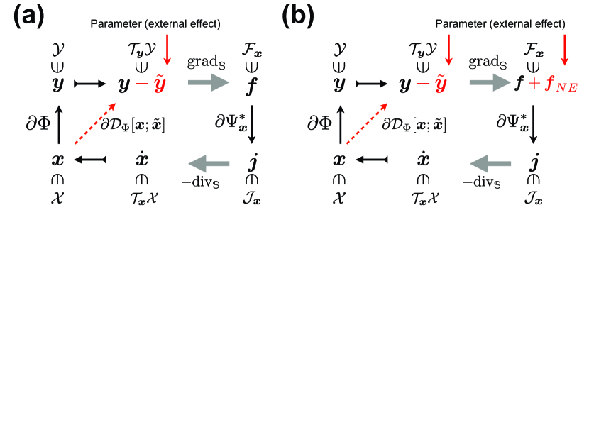
Figure 3: Schematic representation of the equilibrium (a) and nonequilibrium flow (b).

Definition 24 (Equilibrium force, equilibrium flux, and equilibrium flow).

The force generated by the gradient of Bregman divergence associated with a thermodynamic function $\Phi$ is called the (thermodynamic) equilibrium force, and the following equation is denoted as the thermodynamic gradient equation:

$$\bm{f}(\bm{x})=\mathrm{grad}_{\mathbb{S}}\partial\mathcal{D}^{\mathcal{X}}_{\Phi}[\bm{x}\|\tilde{\bm{x}}],$$ (57)

where $\tilde{\bm{x}}\in\mathcal{X}$ is a parameter. The dual of $\bm{f}(\bm{x})$, i.e., $\bm{j}(\bm{x})=\partial\Psi^{*}_{\bm{x}}[\bm{f}(\bm{x})]$, is called the equilibrium flux: A generalized flow $\bm{x}(t)$ is an equilibrium flow if it is driven by the equilibrium force :

$$\dot{\bm{x}}=-\mathrm{div}_{\mathbb{S}}\partial\Psi^{*}_{\bm{x}}[\mathrm{grad}_{\mathbb{S}}\partial\mathcal{D}^{\mathcal{X}}_{\Phi}[\bm{x}\|\tilde{\bm{x}}]].$$ (58)

Using the relation $\partial\mathcal{D}^{\mathcal{X}}_{\Phi}[\bm{x}\|\tilde{\bm{x}}]=\partial\Phi(\bm{x})-\tilde{\bm{y}}$ where $\tilde{\bm{y}}=\partial\Phi(\tilde{\bm{x}})$, Eq. 58 can be rewritten as

$$\dot{\bm{x}}=-\mathrm{div}_{\mathbb{S}}\left[\partial\Psi^{*}_{\bm{x}}\left[\mathrm{grad}_{\mathbb{S}}\left\{\partial\Phi(\bm{x})-\tilde{\bm{y}}\right\}\right]\right],$$ (59)

which explicitly shows the contribution of both the thermodynamic function and the dissipation function to the dynamics (Fig. 3 (a)).

Various properties of the equilibrium flow (Eq. 58) can be obtained from the doubly dual flat structure as we will see in the following sections. In addition, the equilibrium flow captures the properties that the dynamics of thermodynamic equilibrium systems should hold. In this sense, the equilibrium flow is the mathematical representation of the dynamics of equilibrium systems.

Beyond the gradient equilibrium flow, we also consider the non-gradient nonequilibrium flow of the following type:

Definition 25 (Nonequilibrium force and nonequilibrium flow).

The force generated by a shift of the equilibrium force

$$\bm{f}(\bm{x})=\mathrm{grad}_{\mathbb{S}}\partial\mathcal{D}^{\mathcal{X}}_{\Phi}[\bm{x}\|\tilde{\bm{x}}]+\bm{f}_{NE},$$ (60)

is called nonequilibrium force if $\bm{f}_{NE}\not\in\mathrm{Im}[\mathbb{S}^{T}]$. If the shift $\bm{f}_{NE}$ satisfies $\bm{f}_{NE}\in\mathrm{Im}[\mathbb{S}^{T}]$, then $\bm{f}(\bm{x})$ is reduced to the equilibrium force $\bm{f}_{NE}=\bm{0}$ by appropriately changing $\tilde{\bm{x}}$. The nonequilibrium flow is the flow induced by the nonequilibrium force (Fig. 3 (b)):

$$\dot{\bm{x}}=-\mathrm{div}_{\mathbb{S}}\partial\Psi^{*}_{\bm{x}}\left[\left[\mathrm{grad}_{\mathbb{S}}\partial_{\bm{x}}\mathcal{D}^{\mathcal{X}}_{\Phi}[\bm{x}\|\tilde{\bm{x}}]\right]+\bm{f}_{NE}\right].$$ (61)

In the next section, we show that this equation can cover a sufficiently wide class of models, e.g., all types of rLDG and CRN with extended LMA kinetics. Equation 61 can also be associated with nonequilibrium dynamics with a constant environmental force. The techniques in information geometry, Hessian geometry, and convex analysis enable us to investigate such non-gradient dynamics.

Remark 6 (Variational modeling[132]).

We introduced and characterized dynamics based on the thermodynamic functions and dissipation functions. While we employed a restricted definition in order to link dynamics to information geometry, we may further generalize this approach by appropriately choosing the state space, $\bm{f}(\bm{x})$, $\Psi^{*}_{\bm{x}}(\bm{f})$, and $\mathrm{div}_{\mathbb{S}}$. For example, we may consider a $\bm{x}$-dependent and noninteger-valued for the matrix $\mathbb{S}(\bm{x})$. The equilibrium flow may not be restricted to $\mathcal{F}(\bm{x})=\mathcal{D}^{\mathcal{X}}_{\Phi}[\bm{x}\|\tilde{\bm{x}}]$, and the nonequilibrium flow may be defined for $\bm{x}$-dependent $\bm{f}_{NE}(\bm{x})$. This type of approach for modeling dissipative dynamics has been known as variational modeling.

Before closing this section, we mention that the existence of DB states, i.e., $\mathcal{M}^{\mathrm{DB}}\neq\emptyset$, is necessary and sufficient for a nonequilibrium flow to be an equilibrium flow.

Proposition 5 (Detailed balance condition and equilibrium flow).

Consider a flow given by Eq. 61. If $\mathcal{M}^{\mathrm{DB}}\neq\emptyset$, then the flow is equilibrium, i.e., $\bm{f}_{NE}\in\mathrm{Im}\mathbb{S}^{T}$.

Proof.

$\mathcal{M}^{\mathrm{DB}}\neq\emptyset$ means that there exists $\bm{x}_{DB}$ satisfying $\bm{j}(\bm{x}_{DB})=\bm{0}$. Then we have $\bm{j}(\bm{x}_{DB})=\bm{0}\Leftrightarrow\bm{f}(\bm{x}_{DB})=\bm{0}$. If $\bm{f}_{NE}\not\in\mathrm{Im}[\mathbb{S}^{T}]$, $\bm{f}_{NE}\neq\bm{0}$ and thus $\bm{f}(\bm{x})\neq\bm{0}$ for all $\bm{x}\in\mathcal{X}$. Thus, $\bm{f}_{NE}\in\mathrm{Im}[\mathbb{S}^{T}]$ if $\mathcal{M}^{\mathrm{DB}}\neq\emptyset$. ∎

The necessity follows basically from Prop. 3, but we have to show $\mathcal{M}^{\mathrm{ST}}\neq\emptyset$. This will be shown in the following section (Lemma 1).

V Explicit form of thermodynamic and dissipation functions

Before investigating the dynamics of the equilibrium (Eq. 58) and nonequilibrium (Eq. 61) flow, we show how the flow can be associated with the dynamics on graphs and hypergraphs via specific forms of the thermodynamic and dissipation functions. The forms of functions depend on the functional form of the flux that we assume: Eq. 3 for rLDG, Eq. 12 for CRN with LMA kinetics, and Eq. 18 for FPE. It should be noted that the choice of the thermodynamic function and the dissipation function is not unique for a given dynamics in general. Depending on the purpose, we should choose or find an appropriate set of functions.

V.1 Explicit form of thermodynamic functions for rLDG and CRN

For rLDG (Eq. 3) and CRN with LMA kinetics (Eq. 12), the following pair of thermodynamic functions is particularly relevant:

$$\Phi(\bm{x}) :=\left[\ln\bm{x}-\ln\bm{x}^{o}-\bm{1}\right]^{T}\bm{x}=\sum_{i=1}^{N_{\mathbb{X}}}\left[\ln\frac{x_{i}}{x_{i}^{o}}-1\right]x_{i}, \Phi^{*}(\bm{y}) :=(\bm{x}^{o})^{T}e^{\bm{y}}=\sum_{i=1}^{N_{\mathbb{X}}}x_{i}^{o}e^{y_{i}},$$ (62)

which induce the following Legendre transformation:

$$\bm{y} =\partial\Phi(\bm{x})=\ln\bm{x}-\ln\bm{x}^{o}, \bm{x} =\partial\Phi^{*}(\bm{y})=\bm{x}^{o}\circ e^{\bm{y}}.$$ (63)

Here, $\mathcal{Y}=\mathbb{R}^{N_{\mathbb{X}}}$, and $\bm{x}^{o}\in\mathcal{X}$ is a parameter determining the point in $\mathcal{X}$ that is associated with the origin of $\mathcal{Y}$ via the Legendre transformation. For these thermodynamic functions, the Bregman divergence is reduced to the generalized Kullback-Leibler divergence.

$$\mathcal{D}^{\mathcal{X}}[\bm{x}\|\bm{x}^{\prime}]=\left(\ln\frac{\bm{x}}{\bm{x}^{\prime}}\right)^{T}\bm{x}-\bm{1}^{T}(\bm{x}-\bm{x}^{\prime}).$$ (64)

These thermodynamic functions and the Bregman divergence are separable.

If we choose $\bm{x}^{o}=\bm{1}$, then the conventional dual representation for the probability density $\bm{p}$ on a discrete space is recovered:

$$\Phi(\bm{p}) =\left[\ln\bm{p}-\bm{1}\right]^{T}\bm{p}, \Phi^{*}(\bm{y}) =\bm{1}^{T}e^{\bm{y}}, \bm{y} =\partial_{\bm{p}}\Phi(\bm{p})=\ln\bm{p}, \bm{p} =\partial_{\bm{y}}\Phi^{*}(\bm{y})=e^{\bm{y}}.$$ (65)

In this case, $\mathcal{Y}$ is the space of the logarithm of $\bm{p}$. These representations hold even if $\bm{p}$ is not a probability density. If $\bm{p}$ satisfies $\bm{1}^{T}\bm{p}=1$, the generalized KL divergence becomes the normal KL divergence $\mathcal{D}^{\mathcal{X}}[\bm{p}\|\bm{p}^{\prime}]=\left(\ln\frac{\bm{p}}{\bm{p}^{\prime}}\right)^{T}\bm{p}$.

V.2 Explicit form of dissipation functions for rLDG and CRN

To determine the dissipation functions, we need the definition of force, which may depend on the phenomena and purpose. In physics, the flux-force relations, which are also called constitutive equations[133], are central because they determine what kind of change is induced by an incurred force . For rMJP and CRNs, the flux and force are conventionally defined using the one-way fluxes, $\bm{j}^{+}(\bm{x})$ and $\bm{j}^{-}(\bm{x})$ as

$$\bm{j} =\bm{j}^{+}-\bm{j}^{-}, \bm{f} =\ln\bm{j}^{+}-\ln\bm{j}^{-},$$ (66)

where the dependency of $\bm{j}^{\pm}(\bm{x})$ on $\bm{x}$ is abbreviated for notational simplicity. In physics, assuming this form of force-flux relation goes by the name of the local detailed balance (LDB) assumption, or the generalized detailed balance assumption. By defining the frenetic activity [136]:

$$\bm{\omega}:=2\sqrt{\bm{j}^{+}\circ\bm{j}^{-}}\in\mathbb{R}_{\geq 0}^{N_{\mathbb{e}}},,$$ (67)

we have a relation $\bm{j}=\bm{\omega}\circ\left[\frac{\exp(\bm{f}/2)-\exp(-\bm{f}/2)}{2}\right]$. For a fixed $\bm{\omega}$, this relation between the pair $(\bm{j},\bm{f})$ is a one-to-one Legendre duality induced by the following specific form of dissipation functions:

$$\begin{split}\Psi^{*}_{\bm{\omega}}(\bm{f})&:=2\bm{\omega}^{T}\left[\cosh(\bm{f}/2)-\bm{1}\right],\\ \Psi_{\bm{\omega}}(\bm{j})&:=2\bm{\omega}^{T}\left(\mathrm{diag}\left[\frac{\bm{j}}{\bm{\omega}}\right]\sinh^{-1}\left(\frac{\bm{j}}{\bm{\omega}}\right)-\left[\sqrt{\bm{1}+\left(\frac{\bm{j}}{\bm{\omega}}\right)^{2}}-\bm{1}\right]\right),\end{split}$$ (68)

which lead to the Legendre transformation:

$$\bm{j} =\partial\Psi^{*}_{\bm{\omega}}(\bm{f})=\bm{\omega}\circ\sinh(\bm{f}/2), \bm{f} =\partial\Psi_{\bm{\omega}}(\bm{j})=2\sinh^{-1}\left(\frac{\bm{j}}{\bm{\omega}}\right).$$ (69)

We can easily verify that these functions satisfy the conditions for dissipation functions, i.e., Eq. 34, Eq. 35, and Eq. 33.

For the flux $\bm{j}_{\mathrm{MA}}(\bm{x})$ of LMA kinetics (Eq. 12), the force and activity become

$$\bm{f}_{\mathrm{MA}}(\bm{x};\bm{K}) =\left[\ln\bm{K}+\mathbb{S}^{T}\ln\bm{x}\right], \bm{\omega}_{\mathrm{MA}}(\bm{x};\bm{\kappa}) =2\bm{\kappa}\circ\bm{x}^{[{\mathchoice{\raisebox{0.0pt}{\scalebox{1.0}[-1.0]{$\displaystyle\mathbb{L}$}}}{\raisebox{0.0pt}{\scalebox{1.0}[-1.0]{$\textstyle\mathbb{L}$}}}{\raisebox{0.0pt}{\scalebox{1.0}[-1.0]{$\scriptstyle\mathbb{L}$}}}{\raisebox{0.0pt}{\scalebox{1.0}[-1.0]{$\scriptscriptstyle\mathbb{L}$}}}}(B^{+}+B^{-})]^{T}/2}.$$ (70)

where we introduced a transformation of the kinetic parameters $(\bm{k}^{+},\bm{k}^{-})$ into the force part $\bm{K}$ and activity part $\bm{\kappa}$ as $\bm{\kappa}:=\sqrt{\bm{k}^{+}\circ\bm{k}^{-}}$ and $\bm{K}:=\bm{k}^{+}/\bm{k}^{-}$. Because $\bm{k}^{\pm}=\bm{\kappa}\circ\bm{K}^{\pm 1/2}$ holds, $(\bm{\kappa},\bm{K})$ has the same information as $(\bm{k}^{+},\bm{k}^{-})$. Moreover, we can verify that the force and activity are dependent only on $\bm{K}$ and $\bm{\kappa}$, respectively. The dissipation functions of the forms above and their relations to rLDG and CRN were derived from the large deviation function of the corresponding microscopic stochastic models[75, 137]. Actually, the Bregman divergence $\mathcal{D}_{\bm{x}}^{\mathcal{J}}[\bm{j};\bm{j}_{\mathrm{MA}}(\bm{x})]$ of the dissipation functions is identical to the rate function of the flux for rMJP and CRN. Thus, these dissipation functions are keystones connecting macroscopic and microscopic dynamics.

If there exists $\tilde{\bm{y}}$ satisfying $-\mathbb{S}^{T}\tilde{\bm{y}}=\ln\bm{K}$, i.e., $\ln\bm{K}\in\mathrm{Im}\mathbb{S}^{T}$, the force in Eq. 70 is represented as

$$\bm{f}_{\mathrm{MA}}(\bm{x};\bm{K}) =\mathrm{grad}_{\mathbb{S}}\left(\ln\frac{\bm{x}}{\tilde{\bm{x}}}\right)=\mathrm{grad}_{\mathbb{S}}\partial_{\bm{x}}\mathcal{D}^{\mathcal{X}}[\bm{x}\|\tilde{\bm{x}}]\in\mathrm{Im}\mathbb{S}^{T},$$ (71)

where $\tilde{\bm{x}}$ is the Legendre conjugate of $\tilde{\bm{y}}$. Thus, CRN (and rMJP) is an equilibrium flow of the generalized KL divergence $\mathcal{D}^{\mathcal{X}}[\bm{x}\|\tilde{\bm{x}}]$ when the parameter $\bm{K}$ satisfies $\ln\bm{K}\in\mathrm{Im}\mathbb{S}^{T}$. In chemistry, the condition $\ln\bm{K}\in\mathrm{Im}\mathbb{S}^{T}$ is called Wegscheider’s equilibrium condition[138, 47], and the CRN satisfying this parametric condition is called equilibrium CRN . Even if $\ln\bm{K}\in\mathrm{Im}\mathbb{S}^{T}$ is not satisfied, we can represent $\ln\bm{K}=-\mathbb{S}^{T}\tilde{\bm{y}}+\bm{f}_{NE}$ with $\bm{f}_{NE}\not\in\mathrm{Im}\mathbb{S}^{T}$. The force in Eq. 70 is always represented as

$$\bm{f}_{\mathrm{MA}}(\bm{x};\bm{K}) =\mathrm{grad}_{\mathbb{S}}\left(\ln\frac{\bm{x}}{\tilde{\bm{x}}}\right)+\bm{f}_{NE}=\left[\mathrm{grad}_{\mathbb{S}}\left[\partial_{\bm{x}}\mathcal{D}^{\mathcal{X}}[\bm{x}\|\tilde{\bm{x}}]\right]+\bm{f}_{NE}\right],$$ (72)

which leads to the nonequilibrium flow (Eq. 61). Thus, CRN with LMA kinetics as well as rLDG are generally within the class of Eq. 61.

Example 2 (Simplified Brusselator CRN[8, 107] (continued)).

For the Brusselator CRN introduced in Ex. 1, the force and activity defined in Eq. 70 can be explicitly represented as

$$\bm{f}(\bm{x}) =\overbrace{\begin{pmatrix}\ln(k_{1}^{+}/k_{1}^{-})\\ \ln(k_{2}^{+}/k_{2}^{-})\\ \ln(k_{3}^{+}/k_{3}^{-})\\ \end{pmatrix}}^{\ln\bm{K}}+\overbrace{\begin{pmatrix}-\ln x_{1}\\ \ln x_{1}-\ln x_{2}\\ \ln x_{2}-\ln x_{1}\end{pmatrix}}^{\mathbb{S}^{T}\ln\bm{x}}, \bm{\omega}(\bm{x}) =2\overbrace{\begin{pmatrix}\sqrt{k_{1}^{+}k_{1}^{-}}\\ \sqrt{k_{2}^{+}k_{2}^{-}}\\ \sqrt{k_{3}^{+}k_{3}^{-}}\\ \end{pmatrix}}^{\bm{\kappa}}\circ\overbrace{\begin{pmatrix}\sqrt{x_{1}}\\ \sqrt{x_{1}x_{2}}\\ \sqrt{x_{1}^{5}x_{2}}\end{pmatrix}}^{\bm{x}^{[{\mathchoice{\raisebox{0.0pt}{\scalebox{1.0}[-1.0]{$\displaystyle\mathbb{L}$}}}{\raisebox{0.0pt}{\scalebox{1.0}[-1.0]{$\textstyle\mathbb{L}$}}}{\raisebox{0.0pt}{\scalebox{1.0}[-1.0]{$\scriptstyle\mathbb{L}$}}}{\raisebox{0.0pt}{\scalebox{1.0}[-1.0]{$\scriptscriptstyle\mathbb{L}$}}}}(B^{+}+B^{-})]^{T}/2}}.$$ (73)

Remark 7 (Wegscheider’s equilibrium condition and Detailed balance condition).

While we defined equilibrium flow by the specific functional form of force and obtained Wegscheider’s equilibrium condition as the necessary and sufficient condition to have the equilibrium force under LMA kinetics, the equilibrium dynamics is often defined by the existence of the steady state satisfying the DB condition (Eq. 47) in CRN theory. In addition, the DB condition is also often assumed in statistics when we design or analyze a random walk in parameter spaces, e.g., in the Markov Chain Monte Carlo (MCMC) simulations or in other random-walk-based optimization schemes. These two are equivalent for (extended) LMA kinetics. Actually, $\mathcal{M}^{\mathrm{DB}}\neq\emptyset$ means that there exists $\bm{x}_{DB}\in\mathcal{X}$ such that $\bm{j}_{MA}(\bm{x}_{DB})=\bm{0}\Leftrightarrow-\mathbb{S}^{T}\ln\bm{x}_{DB}=\ln\bm{K}$. From the Fredholm alternative, we obtain the Wegscheider’s equilibrium condition $\ln\bm{K}\in\mathrm{Im}\mathbb{S}^{T}$ for the existence of $\bm{x}_{DB}$.

Remark 8 (Linear graph Laplacian dynamics).

The linear graph Laplacian dynamics defined by Eq. 22 can be formally regarded as a generalized flow. From the form of the graph Laplacian (Eq. 21), it is easy to see that Eq. 22 coincides with Eq. 58 if

$$\Phi(\bm{x}) =\frac{1}{2}\langle\bm{x},M_{0}\bm{x}\rangle, \Psi^{*,q}_{\bm{x}}(\bm{f}) =\frac{1}{2}\langle\bm{f},M^{1}\bm{f}\rangle,$$ (74)

where $M_{0}=I$, $M^{1}=\mathrm{diag}[\bm{k}]$, and $\tilde{\bm{x}}=\bm{0}$. In contrast to rLDG, the natural state space and the corresponding dual is $\mathcal{X}=\mathcal{Y}=\mathbb{R}^{N_{\mathbb{v}}}$. In [23], non-quadratic general $\Phi(\bm{x})$ is considered as a class of nonlinear diffusion on a network from information geometric viewpoint.

V.3 Some remarks on the dissipation functions for rLDG and CRN

The dissipation functions in Eq. 68 have several notable properties. First, they are separable:

$$\Psi^{*}_{\bm{\omega}(\bm{x})}(\bm{f}) =\sum_{e=1}^{N_{\mathbb{e}}}\omega_{e}(\bm{x})\psi^{*}(f_{e}), \Psi_{\bm{\omega}(\bm{x})}(\bm{j}) =\sum_{e=1}^{N_{\mathbb{e}}}\omega_{e}(\bm{x})\psi(j_{e}/\omega_{e}(\bm{x})),$$ (75)

where

$$\psi^{*}(f) :=2\left[\cosh(f/2)-1\right]\in[0,\infty),$$ (76)

$$\psi(j) :=2\left(j\sinh^{-1}\left(j\right)-\left[\sqrt{\bm{1}+\bar{j}^{2}}-1\right]\right)\in[0,\infty).$$ (77)

and $\bm{\omega}(\bm{x})$ is local: $\omega_{e}(\bm{x})=2\kappa_{e}\prod_{i=1}^{N_{\mathbb{X}}}x_{i}^{(\gamma^{+}_{i,e}+\gamma^{-}_{i,e})/2}$. The thermodynamic functions in Eq. 62 are also separable.

Second, the scalar function $\psi^{*}(f)$ is the N-function. The N-function of the $(\cosh(f)-1)$-type and the associated Orlicz space have been employed for establishing the infinite-dimensional information geometry by Pistone[139, 140, 72]. In functional analysis, the Orlicz space is a generalization of the $L^{p}$ spaces, which arise naturally when we work on the $L\log^{+}L$ space for the divergences and large deviation functions. Hence, the dissipation functions in Eq. 68 are tightly related to such topics.

Third, various information geometric measures and quantities are related to the dissipation functions in Eq. 68 and also to the associated quantities as follows:

$$\frac{1}{4}\Psi^{*}_{\bm{\omega}}(\bm{f}) =\frac{1}{2}\sum_{e=1}^{N_{\mathbb{e}}}\left[\sqrt{j_{e}^{+}}-\sqrt{j_{e}^{-}}\right]^{2}=:\mathcal{D}_{Hel}[\bm{j}^{+};\bm{j}^{-}]^{2}$$ (78)

$$\frac{1}{2}\bm{1}^{T}\bm{\omega} =\sum_{e=1}^{N_{\mathbb{e}}}\sqrt{j_{e}^{+}j_{e}^{+}}=:\mathrm{BC}[\bm{j}^{+};\bm{j}^{-}]$$ (79)

$$\langle\bm{j},\bm{f}\rangle =\sum_{e=1}^{N_{\mathbb{e}}}(j^{+}_{e}-j^{-}_{e})\ln\frac{j^{+}_{e}}{j^{-}_{e}}=:\mathcal{D}_{Jef}[\bm{j}^{+};\bm{j}^{-}],$$ (80)

where $\mathcal{D}_{Hel}[\bm{j}^{+};\bm{j}^{-}]$, $\mathrm{BC}[\bm{j}^{+};\bm{j}^{-}]$, and $\mathcal{D}_{Jef}[\bm{j}^{+};\bm{j}^{-}]$ are the Hellinger–Kakutani distance, the Bhattacharyya coefficient, and the Jeffreys divergence (symmetrized KL divergence) for $\bm{j}^{+}$ and $\bm{j}^{-}$, respectively. In addition, in physics, the bilinear pairing $\langle\bm{j},\bm{f}\rangle$ of a Legendre dual pair and its approximation using the Hessian matrix are often referred to as the entropy production rate (EPR) $\dot{\Sigma}$ and pseudo-entropy production rate (pEPR) $\dot{\Sigma}^{p}$, respectively[141, 83]:

$$\dot{\Sigma} :=\langle\bm{j},\bm{f}\rangle=\sum_{e=1}^{N_{\mathbb{e}}}(j^{+}_{e}-j^{-}_{e})\ln\frac{j^{+}_{e}}{j^{-}_{e}}.$$ (81)

$$\dot{\Sigma}^{p} :=\langle\bm{j},G_{\bm{\omega},\bm{j}}\bm{j}\rangle=2\sum_{e=1}^{N_{\mathbb{e}}}\frac{(j^{+}_{e}-j^{-}_{e})^{2}}{j^{+}_{e}+j^{-}_{e}},$$ (82)

where we treat $\bm{j}\in\mathcal{J}_{\bm{x}}$ as a member of $\mathcal{T}_{\bm{j}}\mathcal{J}_{\bm{x}}$ by the isomorphism: $\mathcal{J}_{\bm{x}}\cong\mathcal{T}_{\bm{j}}\mathcal{J}_{\bm{x}}\cong C_{1}(\mathbb{H})$. The pEPR $\dot{\Sigma}^{p}$ is an approximation of EPR by replacing $\bm{f}=\partial\Psi_{\bm{\omega}}(\bm{j})$ with $G_{\bm{\omega},\bm{j}}\bm{j}$ and works as a lower bound of $\dot{\Sigma}$: $\dot{\Sigma}\geq\dot{\Sigma}^{p}$[141].

Finally, the dissipation functions in Eq. 68 are not the unique choice to reproduce the force-flux relation in Eq. 66. The quadratic dissipation functions $\Psi^{q,*}_{\bm{x}}(\bm{f}):=\frac{1}{2}\langle\bm{f},M^{*}_{\bm{x}}\bm{f}\rangle$ in Eq. 43 with the following diagonal metric tensor can reproduce the relation in Eq. 66:

$$M^{*}_{\bm{x}}=\mathrm{diag}\left[\frac{\bm{j}^{+}(\bm{x})-\bm{j}^{-}(\bm{x})}{\ln\bm{j}^{+}(\bm{x})-\ln\bm{j}^{-}(\bm{x})}\right]=\mathrm{diag}\left[\left(\frac{j^{+}_{e}(\bm{x})-j^{-}_{e}(\bm{x})}{\ln j^{+}_{e}(\bm{x})-\ln j^{-}_{e}(\bm{x})}\right)_{e}\right].$$ (83)

This type of quadratic dissipation function was proposed even earlier than the non-quadratic ones[142, 143, 144] and has been investigated[145, 107, 146]. Its advantage is that the induced geometry is Riemannian, and thus the information geometric argument is not necessarily required. In addition, this Riemannian geometric structure is analogous to the formal Riemannian geometric structure of FPE and other diffusion processes on continuous manifolds induced via the $L^{2}$-Wasserstein geometry[65, 66] (Fig. 4). Thus, this quadratic dissipation function provides a consistent extension of these results for FPE and diffusion processes to graphs and hypergraphs. Nevertheless, the doubly dual flat structure with the non-quadratic dissipation functions that we introduce is also another sound generalization of the formal Riemannian geometry of FPE, as we see in the next subsection.

As long as we focus only on the trajectory of the generalized flow (Eq. 45), the difference does not matter because both induce the same dynamics. However, the Bregman divergence of the quadratic dissipation functions is not directly related to the rate function of the microscopic stochastic models, while that of nonquadratic ones in Eq. 68 is[137]. Thus, if we consider projections of fluxes and forces in the edge spaces, different choices of dissipation functions lead to different projections. In addition, for non-quadratic dissipation functions, the contributions of the kinetic parameters $\bm{k}^{\pm}$ can be clearly separated into the force part $\bm{K}$ and the activity part $\bm{\kappa}$ in the case of CRN with the LMA kinetics (Eq. 70). This separation enables a physical realization of the projected flux as we derive in the following section.

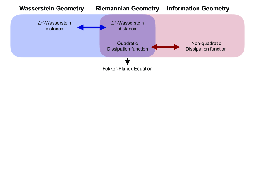
Figure 4: A relationship between Wasserstein geometry and information geometry. The formal Riemannian geometric structure appears at their intersection. It should be noted that, while the regions of $L^{p}$-Wasserstein distance for $p\neq 2$ and nonquadratic dissipation function are not overlapping in this figure, this does not mean that they are unrelated. There may be undiscovered relations between these two regions.

V.4 Explicit forms of thermodynamic and dissipation functions for FPE

For FPE, the dualistic representation of the density $p(\bm{r})$ and its logarithm $y(\bm{r})=\ln p(\bm{r})$ is also relevant. This duality is induced formally by the following thermodynamic functions:

$$\Phi[p] =\int[\ln p(\bm{r})-\bm{1}]p(\bm{r})\mathrm{d}\bm{r}, \Phi^{*}[y] =\int e^{y(\bm{r})}\mathrm{d}\bm{r},$$ (84)

the Legendre transformations of which are

$$y(\bm{r}) =\frac{\delta\Phi[p]}{\delta p}=\ln p(\bm{r}), p(\bm{r}) =\frac{\delta\Phi^{*}[y]}{\delta y}=e^{y(\bm{r})}.$$ (85)

The Bregman divergence becomes the KL divergence $\mathcal{D}_{\mathcal{X}}[p\|p^{\prime}]=\int\mathrm{d}\bm{r}p(\bm{r})\ln\frac{p(\bm{r})}{p^{\prime}(\bm{r})}$. In physics, the flux and force for FPE are defined conventionally as

$$\bm{j}_{\mathrm{FP}}[p(\bm{r})] =D_{0}p(\bm{r})\left\{\bm{F}(\bm{r})/D_{0}-\nabla\ln p(\bm{r})\right\},$$ (86)

$$\bm{f}_{\mathrm{FP}}[p(\bm{r})] =D^{-1}_{0}\bm{F}(\bm{r})-\nabla\ln p(\bm{r}).$$ (87)

The dissipation functions associated with the force-flux relation above are

$$\Psi^{\mathrm{FP},*}_{\bm{\omega}[p]}[\bm{f}] =\frac{1}{2}\int\bm{f}(p(\bm{r}))^{T}M^{*}_{p(\bm{r})}\bm{f}(p(\bm{r}))\mathrm{d}\bm{r}, \Psi^{\mathrm{FP}}_{\bm{\omega}[p]}[\bm{j}] =\frac{1}{2}\int\bm{j}(p(\bm{r}))^{T}M_{p(\bm{r})}\bm{j}(p(\bm{r}))\mathrm{d}\bm{r},$$ (88)

where $M^{*}_{p(\bm{r})}:=\mathrm{diag}[\bm{\omega}[p(\bm{r})]]$, $M_{p(\bm{r})}:=(M^{*}_{p(\bm{r})})^{-1}$, and $\omega_{i}[p(\bm{r})]=D_{0}p(\bm{r})$. Thus, the dissipation functions are formally quadratic and positive definite. If $\bm{F}(\bm{r})$ is a gradient of $U(\bm{r})$ as $\bm{F}(\bm{r})=D_{0}\nabla U(\bm{r})$, $\bm{f}_{\mathrm{FP}}[p(\bm{r})]=-\nabla\ln\frac{p(\bm{r})}{\tilde{p}(\bm{r})}$ holds where $\tilde{p}(\bm{r}):=\exp[U(\bm{r})]$. Then, the dissipation functions, the bilinear pairing $\langle\bm{j}_{\mathrm{FP}},\bm{f}_{\mathrm{FP}}\rangle$, the EPR $\dot{\Sigma}_{\mathrm{FP}}$ in Eq. 81, and the pEPR $\dot{\Sigma}^{p}_{\mathrm{FP}}$ in Eq. 82 formally consolidate into the same quantity:

$$2\Psi^{\mathrm{FP},*}_{\bm{\omega}[p]}[\bm{f}_{\mathrm{FP}}]=2\Psi^{\mathrm{FP}}_{\bm{\omega}[p]}[\bm{j}_{\mathrm{FP}}]=\langle\bm{j}_{\mathrm{FP}},\bm{f}_{\mathrm{FP}}\rangle=\dot{\Sigma}_{\mathrm{FP}}=\dot{\Sigma}^{p}_{\mathrm{FP}}=D_{0}\int p(\bm{r})\left(\nabla_{\bm{r}}\ln\frac{p(\bm{r})}{\tilde{p}(\bm{r})}\right)^{2}\mathrm{d}\bm{r}.$$ (89)

The last quantity without $D_{0}$ is known as relative Fisher information[66, 147] and Hyvärinen divergence[148, 124] between $p$ and $\tilde{p}$. For $U(\bm{f})=0$, it reduces to the Fisher information number $\mathbb{I}_{F}[p]$ in Eq. 1. This consolidation is a source of confusion, because the same quantity for FPE or linear diffusion processes has different names in different contexts and in different disciplines. However, they actually have different definitions, roles, and meanings, which becomes explicit in the information-geometric formulation.

VI Orthogonal subspaces, dual foliation, and Pythagorean relation

To investigate the behaviors and properties of the equilibrium (Eq. 58) and nonequilibrium (Eq. 61) flow, especially its topological and algebraic constraints from the graph or hypergraph structure, information geometry provides the ideal tools. In particular, the four affine subspaces associated with the cycle and cocycle subspaces of the chain and cochain complexes (Fig. 5) form dual foliations via the Legendre transformation, whose geometric properties are captured by information geometry[149, 1]. It should be noted that the results of this section do not assume the specific forms of the thermodynamic and dissipation functions introduced in Sec. V.

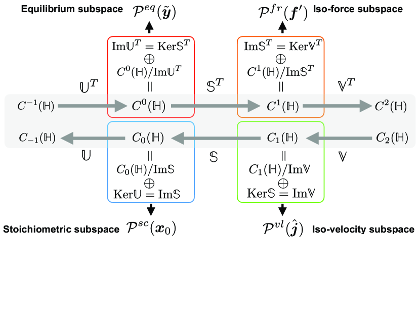
Figure 5: Diagrammatic representation of the four subspaces and their relationship with the chain and cochain complexes of $\mathbb{H}$.

VI.1 Four affine subspaces

Two families of orthogonally complement affine subspaces are naturally introduced on $\mathcal{X}$ and $\mathcal{Y}$, respectively, from the topological structure of graph and hypergraph, i.e., $\mathbb{B}$ and $\mathbb{S}$.

Definition 26 (Stoichiometric subspaces in $\mathcal{X}$).

The stoichiometric subspaces are defined as

$$\mathcal{P}^{sc}(\bm{x}_{0}) :=\{\bm{x}\in\mathcal{X}|\bm{x}-\bm{x}_{0}\in\mathrm{Im}\mathbb{S}\},\quad\bm{x}_{0}\in\mathcal{X}$$ (90)

where $\bm{x}_{0}$ is a parameter to specify the position of the subspace (Fig. 5, lower left).

Definition 27 (Equilibrium subspaces in $\mathcal{Y}$).

The equilibrium subspaces (Fig. 5, upper left) are defined as

$$\mathcal{P}^{eq}(\tilde{\bm{y}}) :=\left\{\bm{y}\in\mathcal{Y}|\bm{y}-\tilde{\bm{y}}\in\mathrm{Ker}\mathbb{S}^{T}\right\},\quad\tilde{\bm{y}}\in\mathcal{Y}.$$ (91)

$\mathcal{P}^{sc}(\bm{x}_{0})$ and $\mathcal{P}^{eq}(\tilde{\bm{y}})$ are of orthogonal complement to each other: $\langle\bm{x}-\bm{x}_{0},\bm{y}^{\prime}-\tilde{\bm{y}}\rangle=0$ for $\bm{x}\in\mathcal{P}^{sc}(\bm{x}_{0})$ and $\bm{y}^{\prime}\in\mathcal{P}^{eq}(\tilde{\bm{y}})$. Because $\mathbb{S}$ and $\mathbb{S}^{T}$ are the discrete differentials, $\delta_{1}$ and $\delta^{0}$, $\mathcal{P}^{sc}(\bm{x}_{0})$ and $\mathcal{P}^{eq}(\tilde{\bm{y}})$ are associated with the $0$-cycle and $0$-cocycle spaces, respectively.

Two other families of orthogonal-complement subspaces are introduced on $\mathcal{J}_{\bm{x}}$ and $\mathcal{F}_{\bm{x}}$.

Definition 28 (Iso-velocity subspaces in $\mathcal{J}_{\bm{x}}$).

The iso-velocity subspaces (Fig. 5, lower right) are defined as

$$\mathcal{P}^{vl}(\hat{\bm{j}})=\left\{\bm{j}\in\mathcal{J}_{\bm{x}}|\bm{j}-\hat{\bm{j}}\in\mathrm{Ker}\mathbb{S}\right\},\qquad\hat{\bm{j}}\in\mathcal{J}_{\bm{x}}.$$ (92)

Definition 29 (Iso-force subspaces in $\mathcal{F}_{\bm{x}}$).

The iso-external-force subspaces, iso-force subspaces in short, (Fig. 5, upper right) are defined as

$$\mathcal{P}^{fr}(\bm{f}^{\prime}):=\left\{\bm{f}\in\mathcal{F}_{\bm{x}}|\bm{f}-\bm{f}^{\prime}\in\mathrm{Im}\mathbb{S}^{T}\right\},\qquad\bm{f}^{\prime}\in\mathcal{F}_{\bm{x}}.$$ (93)

Again, from the correspondence of $\delta_{1}=\mathbb{S}$ and $\delta^{0}=\mathbb{S}^{T}$, $\mathcal{P}^{vl}(\hat{\bm{j}})$ and $\mathcal{P}^{fr}(\bm{f}^{\prime})$ are associated with the $1$-cycle and $1$-cocycle spaces, respectively. We specifically call $\mathcal{P}^{vl}(\bm{0})$ and $\mathcal{P}^{fr}(\bm{0})$ zero-velocity subspace and equilibrium force subspace, respectively.

VI.2 Meaning of the subspaces

All four subspaces are natural constituents in the theory of algebraic graph theory and homological algebra. Here, we provide their meaning in terms of the dynamics on graphs and hypergraphs.

The stoichiometric and iso-velocity subspaces, $\mathcal{P}^{sc}(\bm{x}_{0})$ and $\mathcal{P}^{vl}(\hat{\bm{j}})$, are related by the continuity equation (Eq. 10). From the continuity equation, $\mathcal{P}^{vl}(\hat{\bm{j}})$ is the set of fluxes that induce the same velocity as a reference $\hat{\bm{j}}$ does: $\bm{j}\in\mathcal{P}^{vl}(\hat{\bm{j}})\Longleftrightarrow\dot{\bm{x}}=-\mathbb{S}\hat{\bm{j}}=-\mathbb{S}\bm{j}$. Thereby, $\mathcal{P}^{vl}(\hat{\bm{j}})$ is parametrized as follows:

$$\mathcal{P}^{vl}(\dot{\bm{x}}) =\{\bm{j}\in\mathcal{J}_{\bm{x}}|-\mathbb{S}\bm{j}=\dot{\bm{x}}\},\quad\dot{\bm{x}}\in\mathrm{Im}[\mathbb{S}]=\mathrm{Ker}[\mathbb{U}],$$ (94)

This subspace is crucial to characterize fluxes that can realize the same dynamics as the reference one.

The stoichiometric subspace $\mathcal{P}^{sc}(\bm{x}_{0})$ determines the subspace in which the dynamics are algebraically constrained via the topology of the underlying graph or hypergraph. Because $\dot{\bm{x}}=-\mathbb{S}\bm{j}(\bm{x}(t))$, for an initial state $\bm{x}(0)=\bm{x}_{0}$, $\bm{x}(t)-\bm{x}_{0}\in\mathrm{Im}[\mathbb{S}]$ should hold, meaning that $\bm{x}(t)\in\mathcal{P}^{sc}(\bm{x}_{0})$. Thus, $\mathcal{P}^{sc}(\bm{x}_{0})$ is the subspace in which the dynamics are restricted by the initial condition $\bm{x}_{0}$. $\mathcal{P}^{sc}(\bm{x}_{0})$ can also be represented parametrically by the quantities which are conserved by the dynamics. For any vector $\bm{u}\in\mathrm{Ker}\mathbb{S}^{T}$, $\eta(t):=\bm{u}^{T}\bm{x}(t)$ is constant over time:

$$\dot{\eta}(t)=\frac{\mathrm{d}\bm{u}^{T}\bm{x}(t)}{\mathrm{d}t}=\bm{u}^{T}\frac{\mathrm{d}\bm{x}(t)}{\mathrm{d}t}=-\bm{u}^{T}\mathbb{S}\bm{j}(\bm{x})=0.$$ (95)

In Sec. III.1, we defined a matrix $\mathbb{U}$ by a complete basis of $\mathrm{Ker}\mathbb{S}^{T}$ so that $\mathrm{Im}\mathbb{U}^{T}=\mathrm{Ker}\mathbb{S}^{T}$. Using $\mathbb{U}$, the conserved quantities for a given initial condition $\bm{x}_{0}$ are obtained as $\bm{\eta}=\mathbb{U}\bm{x}_{0}=\mathbb{U}\bm{x}(t)$. Because $\mathrm{Im}\mathbb{U}$ is isomorphic to $C_{-1}(\mathbb{H})$, the stoichiometric subspace is explicitly parametrized by the conserved quantities (an element of $C_{-1}(\mathbb{H})$):

$$\mathcal{P}^{sc}(\bm{\eta}) =\{\bm{x}\in\mathcal{X}|\mathbb{U}\bm{x}=\bm{\eta}\},\quad\bm{\eta}\in C_{-1}(\mathbb{H}).$$ (96)

For rMJP, the conserved quantity is reduced to the conservation of probability $\bm{1}\bm{p}(t)=1$ and $\mathcal{P}^{sc}(\bm{p}_{0})$ becomes the probability simplex. Because $\mathrm{Ker}\mathbb{B}^{T}$ determines the connected components of the graph $\mathbb{G}$ and we conventionally assume that the underlying graph is connected in rMJP, we only have the one-dimensional cokernel space and one conserved quantity, which is $\eta=1$. Thus, the conservation of probability or, equivalently, the restriction of $\bm{p}$ in the probability simplex is automatically guaranteed from the topological constraint of the dynamics if we start from the initial state satisfying $\bm{1}^{T}\bm{p}_{0}=1$.

The iso-force subspace $\mathcal{P}^{fr}(\bm{f}^{\prime})$ and the equilibrium subspace $\mathcal{P}^{eq}(\tilde{\bm{y}})$ are related to the equilibrium and nonequilibrium force equations, Eq. 57 and Eq. 60. The equilibrium force defined in Eq. 57 satisfies $\bm{f}(\bm{x})\in\mathrm{Im}\mathbb{S}^{T}=\mathcal{P}^{fr}(\bm{0})$. Thus, the equilibrium-force subspace $\mathcal{P}^{fr}(\bm{0})$ is literally the set of equilibrium forces. $\mathcal{P}^{fr}(\bm{f}^{\prime})$ is its shift by $\bm{f}^{\prime}\in\mathcal{F}_{\bm{x}}$. Using $\mathbb{V}$ defined in Sec. III.1, we can represent $\mathcal{P}^{fr}$ parametrically as

$$\mathcal{P}^{fr}(\bm{\zeta}) =\{\bm{f}\in\mathcal{F}_{\bm{x}}|\mathbb{V}^{T}\bm{f}=\bm{\zeta}\},\quad\bm{\zeta}\in C^{2}(\mathbb{H})$$ (97)

because $\mathcal{F}_{\bm{x}}/\mathrm{Im}\mathbb{S}^{T}\cong\mathcal{F}_{\bm{x}}/\mathrm{Ker}\mathbb{V}^{T}\cong\mathrm{Im}\mathbb{V}^{T}\cong C^{2}(\mathbb{H})$. Thus, $\bm{\zeta}$ characterizes the type of nonequilibrium forces quotient by the equilibrium forces.

Finally, the equilibrium subspace $\mathcal{P}^{eq}(\tilde{\bm{y}})$ can also be regarded as the set of potentials $\bm{y}$ that generate the same equilibrium force because any $\bm{y}\in\mathcal{P}^{eq}(\tilde{\bm{y}})$ satisfies $\bm{f}^{\prime}=\mathbb{S}^{T}\bm{y}=\mathbb{S}^{T}\tilde{\bm{y}}\in\mathcal{P}^{fr}(\bm{0})$. Due to this, the equilibrium subspace $\mathcal{P}^{eq}$ is parameterized as

$$\mathcal{P}^{eq}(\bm{f}^{\prime}) =\{\bm{y}\in\mathcal{Y}|\mathbb{S}^{T}\bm{y}=\bm{f}^{\prime}\},\quad\bm{f}^{\prime}\in\mathrm{Im}[\mathbb{S}^{T}].$$ (98)

The parametric forms of the subspaces are summarized as follows:

$$\mathcal{P}^{vl}(\dot{\bm{x}}) =\{\bm{j}\in\mathcal{J}_{\bm{x}}|-\mathbb{S}\bm{j}=\dot{\bm{x}}\}, \dot{\bm{x}} \in\mathrm{Im}[\mathbb{S}]=\mathrm{Ker}[\mathbb{U}],$$ (99)

$$\mathcal{P}^{sc}(\bm{\eta}) =\{\bm{x}\in\mathcal{X}|\mathbb{U}\bm{x}=\bm{\eta}\}, \bm{\eta} \in\mathrm{Im}[\mathbb{U}]=C_{-1}(\mathbb{H}),$$ (100)

$$\mathcal{P}^{fr}(\bm{\zeta}) =\{\bm{f}\in\mathcal{F}_{\bm{x}}|\mathbb{V}^{T}\bm{f}=\bm{\zeta}\}, \bm{\zeta} \in\mathrm{Im}[\mathbb{V}^{T}]=C^{2}(\mathbb{H}),$$ (101)

$$\mathcal{P}^{eq}(\bm{f}^{\prime}) =\{\bm{y}\in\mathcal{Y}|\mathbb{S}^{T}\bm{y}=\bm{f}^{\prime}\}, \bm{f}^{\prime} \in\mathrm{Im}[\mathbb{S}^{T}]=\mathrm{Ker}[\mathbb{V}^{T}].$$ (102)

From these subspaces, we can obtain dual foliations on the vertex and edge spaces.

VI.3 Dual Manifold, Dual Foliation, and Pythagorean relation in vertex spaces

For the subspaces $\mathcal{P}^{sc}$ and $\mathcal{P}^{eq}$ in the density and potential spaces, we introduce their Legendre transformation via the thermodynamic functions, $\Phi(\bm{x})$ and $\Phi^{*}(\bm{y})$, which form the dual foliation with the subspaces of orthogonal complement (Fig. 6, left).

Figure 6: Diagrammatic representation of the dual foliations in $\mathcal{X}$, $\mathcal{Y}$, $\mathcal{J}_{\bm{x}}$, and $\mathcal{F}_{\bm{x}}$ spaces.

Definition 30 (Stoichiometric manifold in $\mathcal{Y}$ and equilibrium manifold in $\mathcal{X}$).

The stoichiometric and equilibrium manifolds (Fig. 6, left) are defined respectively as

$$\mathcal{M}^{sc}(\bm{y}_{0}) :=\partial\Phi[\mathcal{P}^{sc}(\bm{x}_{0})]\subset\mathcal{Y},\quad\bm{y}_{0}=\partial\Phi(\bm{x}_{0}),$$ (103)

$$\mathcal{M}^{eq}(\tilde{\bm{x}}) :=\partial\Phi^{*}[\mathcal{P}^{eq}(\tilde{\bm{y}})]\subset\mathcal{X},\quad\tilde{\bm{x}}=\partial\Phi^{*}(\tilde{\bm{y}}).$$ (104)

Lemma 1 (Dual foliations in density and potential spaces[85]).

$\mathcal{P}^{sc}$ and $\mathcal{M}^{eq}$ are foliations of $\mathcal{X}$, and $\mathcal{M}^{sc}$ and $\mathcal{P}^{eq}$ are foliations of $\mathcal{Y}$. For each pair of $(x_{0},\tilde{x})$, the intersection of $\mathcal{P}^{sc}(\bm{x}_{0})$ and $\mathcal{M}^{eq}(\tilde{\bm{x}})$ is unique and transversal. The same applies to $\mathcal{M}^{sc}(\bm{y}_{0})$ and $\mathcal{P}^{eq}(\tilde{\bm{y}})$. Then, $(\mathcal{P}^{sc},\mathcal{M}^{eq})$ and $(\mathcal{M}^{sc},\mathcal{P}^{eq})$ form dual foliations (nonlinear coordinate systems) in $\mathcal{X}$ and $\mathcal{Y}$ spaces, respectively.

Proof.

The polyhedron $\mathcal{P}^{sc}(\bm{x}_{0})$ and the affine subspace $\mathcal{P}^{eq}(\tilde{\bm{y}})$ can cover the whole $\mathcal{X}$ and $\mathcal{Y}$ by changing $\bm{x}_{0}$ and $\tilde{\bm{y}}$, respectively. Similarly, $\mathcal{M}^{eq}(\tilde{\bm{x}})$ and $\mathcal{M}^{sc}(\bm{y}_{0})$ can cover the whole $\mathcal{X}$ and $\mathcal{Y}$ because Legendre transformations by the thermodynamic functions are one-to-one between $\mathcal{X}$ and $\mathcal{Y}$. Consider the intersection of $\mathcal{P}^{sc}(\bm{x}_{0})$ and $\mathcal{M}^{eq}(\tilde{\bm{x}})$ in $\mathcal{X}$ space. The condition that $\mathcal{P}^{sc}(\bm{x}_{0})\cap\mathcal{M}^{eq}(\tilde{\bm{x}})\neq\emptyset$ is related to the existence of $\bm{x}^{\dagger}$ defined by the following convex optimization problem:

$$\bm{x}^{\dagger}:=\arg\min_{\bm{x}\in\overline{\mathcal{P}^{sc}(\bm{x}_{0})}}\mathcal{D}^{\mathcal{X}}_{\Phi}[\bm{x}\|\tilde{\bm{x}}].$$ (105)

Because of the properties of $\Phi(\bm{x})$, $\mathcal{D}^{\mathcal{X}}_{\Phi}[\bm{x}\|\tilde{\bm{x}}]$ and its restriction to $\overline{\mathcal{P}^{sc}(\bm{x}_{0})}$ are strictly convex with respect to $\bm{x}$. Thus, $\bm{x}^{\dagger}$ is unique and either satisfies the stationarity condition $\bm{x}^{\dagger}\in\mathcal{P}^{sc}(\bm{x}_{0})\cap\mathcal{M}^{eq}(\tilde{\bm{x}})$ if $\bm{x}^{\dagger}\in\mathcal{P}^{sc}(\bm{x}_{0})$ or locates on the boundary $\partial\mathcal{X}$ if $\bm{x}^{\dagger}\not\in\mathcal{P}^{sc}(\bm{x}_{0})$, where we used $\mathbb{S}^{T}\frac{\partial\mathcal{D}^{\mathcal{X}}[\bm{x}\|\tilde{\bm{x}}]}{\partial\bm{x}}=\bm{0}\Leftrightarrow\mathbb{S}^{T}(\bm{y}-\tilde{\bm{y}})=\bm{0}\Leftrightarrow\bm{y}\in\mathcal{P}^{eq}(\tilde{\bm{y}})\Leftrightarrow\bm{x}\in\mathcal{M}^{eq}(\tilde{\bm{x}})$. Let $\bm{x}_{bd}\in\partial\mathcal{X}$ and $\bm{x}_{in}\in\mathcal{X}$ be arbitrary points on the boundary and interior of $\mathcal{X}$. From the condition Eq. 25 of the thermodynamic function, for $\bm{x}_{\lambda}:=\lambda\bm{x}_{in}+(1-\lambda)\bm{x}_{bd}$ where $\lambda\in[0,1]$,

$$\lim_{\lambda\to+0}\frac{\mathrm{d}\mathcal{D}^{\mathcal{X}}[\bm{x}_{\lambda}\|\tilde{\bm{x}}]}{\mathrm{d}\lambda}=\lim_{\lambda\to+0}\left[\frac{\mathrm{d}\Phi(\bm{x}_{\lambda})}{\mathrm{d}\lambda}-\left\langle\tilde{\bm{y}},\frac{\mathrm{d}\bm{x}_{\lambda}}{\mathrm{d}\lambda}\right\rangle\right]=-\infty.$$ (106)

Thus, $\bm{x}^{\dagger}\not\in\mathcal{X}$ is excluded, and the intersection exists, i.e., $\bm{x}^{\dagger}\in\mathcal{P}^{sc}(\bm{x}_{0})\cap\mathcal{M}^{eq}(\tilde{\bm{x}})$. The intersection $\bm{x}^{\dagger}$ is unique and transversal because $\langle\bm{x}_{sc}-\bm{x}^{\dagger},\bm{y}_{eq}-\bm{y}^{\dagger}\rangle=0$ holds for any $\bm{x}_{sc}\in\mathcal{P}^{sc}(\bm{x}_{0})$ and $\bm{x}_{eq}\in\mathcal{M}^{eq}(\tilde{\bm{x}})$ and the dimensions of $\mathcal{P}^{sc}(\bm{x}_{0})$ and $\mathcal{M}^{eq}(\tilde{\bm{x}})$ are complementary because $\mathcal{P}^{sc}(\bm{x}_{0})$ and $\mathcal{P}^{eq}(\tilde{\bm{y}})$ are of orthogonal complement (see also the proof in [83]). As a result, $\bm{x}^{\dagger}\in\mathcal{P}^{sc}(\bm{x}_{0})\cap\mathcal{M}^{eq}(\tilde{\bm{x}})$ always exists, and $(\mathcal{P}^{sc},\mathcal{M}^{eq})$ forms a dual foliation in $\mathcal{X}$. Also $(\mathcal{M}^{sc},\mathcal{P}^{eq})$ does in $\mathcal{Y}$ because they are bijective Legendre duals of $(\mathcal{P}^{sc},\mathcal{M}^{eq})$. ∎

This result is reduced to Birch’s theorem[101, 103] and the seminal result by Horn and Jackson[41] when the thermodynamic function is the generalized KL divergence.

With the dual foliation, we can consider the generalized Pythagorean relations and orthogonal decomposition. For any three points satisfying $\bm{x}\in\mathcal{P}^{sc}(\bm{x}_{0})$, $\bm{x}_{q}\in\mathcal{M}^{eq}(\tilde{\bm{x}})$, and $\bm{x}^{\dagger}=\mathcal{P}^{sc}(\bm{x}_{0})\cap\mathcal{M}^{eq}(\tilde{\bm{x}})$, we have the generalized Pythagorean relation:

$$\mathcal{D}^{\mathcal{X}}[\bm{x}\|\bm{x}_{q}]=\mathcal{D}^{\mathcal{X}}[\bm{x}\|\bm{x}^{\dagger}]+\mathcal{D}^{\mathcal{X}}[\bm{x}^{\dagger}\|\bm{x}_{q}].$$ (107)

In $\mathcal{Y}$ space, we also have the dual version of the relations as

$$\mathcal{D}^{\mathcal{Y}}[\bm{y}_{q}\|\bm{y}]=\mathcal{D}^{\mathcal{Y}}[\bm{y}_{q}\|\bm{y}^{\dagger}]+\mathcal{D}^{\mathcal{Y}}[\bm{y}^{\dagger}\|\bm{y}].$$ (108)

These relations are used to characterize the steady state of equilibrium and nonequilibrium flow geometrically and also variationally.

Remark 9 (Interpretation in terms of statistical inference).

The meaning of the equilibrium manifold in statistics can be clarified more explicitly by considering the specific form of thermodynamic function (Eq. 65). For this thermodynamic function, the equilibrium manifold $\mathcal{M}^{eq}(\tilde{\bm{p}})$ is represented as

$$\mathcal{M}^{eq}(\tilde{\bm{p}}) =\left\{\bm{p}\in\mathcal{X}|\ln\bm{p}-\ln\tilde{\bm{p}}\in\mathrm{Ker}\mathbb{S}^{T}\right\}=\left\{\bm{p}\in\mathcal{X}|\bm{p}=\tilde{\bm{p}}\circ\exp\left[\mathbb{U}^{T}\bm{\eta}^{*}\right],\bm{\eta}^{*}\in C^{-1}(\mathbb{H})\right\}$$ (109)

where we use the fact $\mathbb{S}^{T}\mathbb{U}^{T}=0$. Thus, $\mathcal{M}^{eq}(\tilde{\bm{p}})$ is an exponential family with algebraic constraints via $\mathbb{U}^{T}$. In contrast, $\mathcal{P}^{sc}(\bm{\eta})$ can be regarded as the data manifold, which constrains $\bm{p}$ by $\bm{\eta}=\mathbb{U}\bm{p}$, because $\mathbb{U}\bm{p}$ can be interpreted as expectation of observables $\{\bm{u}_{\ell}\}_{\ell\in[1,N_{\mathbb{l}}]}$. Thus, the intersection $\bm{p}^{\dagger}=\mathcal{P}^{sc}(\bm{\eta})\cap\mathcal{M}^{eq}(\tilde{\bm{p}})$ is the maximum likelihood estimator. The exponential family with linear algebraic constraints as in Eq. 109 appears in algebraic statistics where $\mathbb{U}$ is sometimes called the design matrix[103].

VI.4 Dual manifold, dual foliation in edge spaces and generalized Helmholtz-Hodge-Kodaira decomposition

For the edge spaces, we similarly introduce the iso-velocity and iso-force manifolds, which are the duals of $\mathcal{P}^{fr}(\bm{f}^{\prime})$ and $\mathcal{P}^{vl}(\hat{\bm{j}})$, respectively, via the Legendre transformations by the dissipation functions, $\Psi_{\bm{x}}(\bm{j})$ and $\Psi^{*}_{\bm{x}}(\bm{f})$ (Fig. 6, right):

Definition 31 (Iso-velocity manifold in $\mathcal{F}_{\bm{x}}$ and iso-force manifold in $\mathcal{J}_{\bm{x}}$).

The iso-velocity and iso-force manifolds (Fig. 6, right) are defined as follows:

$$\mathcal{M}^{vl}_{\bm{x}}(\hat{\bm{f}}) :=\partial\Psi_{\bm{x}}[\mathcal{P}^{vl}(\hat{\bm{j}})]\subset\mathcal{F}_{\bm{x}}, \hat{\bm{f}} =\partial\Psi_{\bm{x}}(\hat{\bm{j}}),$$ (110)

$$\mathcal{M}^{fr}_{\bm{x}}(\bm{j}^{\prime}) :=\partial\Psi^{*}_{\bm{x}}[\mathcal{P}^{fr}(\bm{f}^{\prime})]\subset\mathcal{J}_{\bm{x}}, \bm{j}^{\prime} =\partial\Psi^{*}_{\bm{x}}(\bm{f}^{\prime}).$$ (111)

It should be noted that $\mathcal{M}^{vl}_{\bm{x}}(\hat{\bm{f}})$ and $\mathcal{M}^{fr}_{\bm{x}}(\bm{j}^{\prime})$ are dependent on $\bm{x}$ via the $\bm{x}$ dependence of the dissipation functions. We obtain the intersections in $\mathcal{J}_{\bm{x}}$ and $\mathcal{F}_{\bm{x}}$:

$$\bm{j}^{\dagger} :=\mathcal{P}^{vl}(\hat{\bm{j}})\cap\mathcal{M}^{fr}_{\bm{x}}(\bm{j}^{\prime}), \bm{f}^{\dagger} :=\mathcal{M}^{vl}_{\bm{x}}(\hat{\bm{f}})\cap\mathcal{P}^{fr}(\bm{f}^{\prime}),$$ (112)

which are also unique and transversal for each $\bm{x}\in\mathcal{X}$ because $\mathcal{J}_{\bm{x}}$ and $\mathcal{F}_{\bm{x}}$ are whole vector spaces and the Legendre transformations are one-to-one. Thus, similarly to the case of vertex space, we have the dual foliation:

Lemma 2 (Dual foliations in edge space[83]).

For each $\bm{x}\in X$, $(\mathcal{P}^{vl},\mathcal{M}^{fr}_{\bm{x}})$ and $(\mathcal{M}^{vl}_{\bm{x}},\mathcal{P}^{fr})$ form dual foliations in $\mathcal{J}_{\bm{x}}$ and $\mathcal{F}_{\bm{x}}$ spaces, respectively.

For $\hat{\bm{j}}$ and $\bm{f}^{\prime}$, and their intersections $\bm{j}^{\dagger}$ and $\bm{f}^{\dagger}$ defined in Eq. 112, $\langle\hat{\bm{j}}-\bm{j}^{\dagger},\bm{f}^{\dagger}-\bm{f}^{\prime}\rangle=0$ holds. Thus, we have the generalized Pythagorean relations:

$$\mathcal{D}^{\mathcal{J}}_{\bm{x}}[\hat{\bm{j}}\|\bm{j}^{\prime}] =\mathcal{D}^{\mathcal{J}}_{\bm{x}}[\hat{\bm{j}}\|\bm{j}^{\dagger}]+\mathcal{D}^{\mathcal{J}}_{\bm{x}}[\bm{j}^{\dagger}\|\bm{j}^{\prime}], \mathcal{D}^{\mathcal{F}}_{\bm{x}}[\bm{f}^{\prime}\|\hat{\bm{f}}] =\mathcal{D}^{\mathcal{F}}_{\bm{x}}[\bm{f}^{\prime}\|\bm{f}^{\dagger}]+\mathcal{D}^{\mathcal{F}}_{\bm{x}}[\bm{f}^{\dagger}\|\hat{\bm{f}}].$$ (113)

In contrast to the thermodynamic functions $(\Phi,\Phi^{*})$, the dissipation functions have symmetry, which makes the origins $\bm{0}$ in $\mathcal{J}_{\bm{x}}$ and $\mathcal{F}_{\bm{x}}$ special and leads to an extension of Helmholtz-Hodge-Kodaira decomposition.

Theorem 1 (Information-geometric extension of Helmholtz-Hodge-Kodaira (HHK) decomposition[83]).

For a given flux-force Legendre pair $(\bm{j},\bm{f})\in(\mathcal{J}_{\bm{x}},\mathcal{F}_{\bm{x}})$, we have their unique $\bm{x}$-dependent decompositions:

$$\bm{j} =\bm{j}_{eq}(\bm{x})+(\bm{j}-\bm{j}_{eq}(\bm{x})), \bm{f} =\bm{f}_{st}(\bm{x})+(\bm{f}-\bm{f}_{st}(\bm{x})),$$ (114)

such that $\bm{f}_{eq}(\bm{x})\in\mathcal{P}^{fr}(\bm{0})$, $\bm{j}-\bm{j}_{eq}(\bm{x})\in\mathcal{P}^{vl}(\bm{0})$, $\bm{f}-\bm{f}_{st}(\bm{x}),\in\mathcal{P}^{fr}(\bm{0})$, and $\bm{j}_{st}(\bm{x})\in\mathcal{P}^{vl}(\bm{0})$ hold. In addition, $\bm{j}_{eq}(\bm{x})$ and $\bm{f}_{st}(\bm{x})$ are characterized geometrically as

$$\bm{j}_{eq}(\bm{x}) :=\mathcal{P}^{vl}(\bm{j})\cap\mathcal{M}^{fr}_{\bm{x}}(\bm{0}), \bm{f}_{st}(\bm{x}) :=\mathcal{M}^{vl}_{\bm{x}}(\bm{0})\cap\mathcal{P}^{fr}(\bm{f}).$$ (115)

Furthermore, $\bm{j}_{eq}$ and $\bm{f}_{st}$ are also characterized variationally as the minimizers of dissipation functions:

$$\bm{j}_{eq}(\bm{x}) =\arg\min_{\bm{j}^{\prime}\in\mathcal{P}^{vl}(\bm{j})}\Psi_{\bm{x}}(\bm{j}^{\prime}), \bm{f}_{st}(\bm{x}) =\arg\min_{\bm{f}^{\prime\prime}\in\mathcal{P}^{fr}(\bm{f})}\Psi_{\bm{x}}^{*}(\bm{f}^{\prime\prime}).$$ (116)

Proof.

The uniqueness of $\bm{j}_{eq}(\bm{x})$ and $\bm{f}_{st}(\bm{x})$ as intersections in Eq. 115 follows immediately from the property of the dual foliations. Because, for any $\bm{j}^{\prime}\in\mathcal{P}^{vl}(\bm{j})$ and $\bm{f}^{\prime\prime}\in\mathcal{P}^{fr}(\bm{f})$, $\langle\bm{j}^{\prime}-\bm{j}_{eq},\bm{f}_{eq}\rangle=0$ and $\langle\bm{j}_{st},\bm{f}^{\prime\prime}-\bm{f}_{st}\rangle=0$ hold, the generalized Pythagorean relations lead to

$$\begin{aligned} \mathcal{D}^{\mathcal{J}}_{\bm{x}}[\bm{j}^{\prime}\|\bm{0}]&=\mathcal{D}^{\mathcal{J}}_{\bm{x}}[\bm{j}^{\prime}\|\bm{j}_{eq}]+\mathcal{D}^{\mathcal{J}}_{\bm{x}}[\bm{j}_{eq}\|\bm{0}],&\mathcal{D}^{\mathcal{F}}_{\bm{x}}[\bm{f}^{\prime\prime}\|\bm{0}]&=\mathcal{D}^{\mathcal{F}}_{\bm{x}}[\bm{f}^{\prime\prime}\|\bm{f}_{st}]+\mathcal{D}^{\mathcal{F}}_{\bm{x}}[\bm{f}_{st}\|\bm{0}].\end{aligned}$$

Because $\mathcal{D}^{\mathcal{J}}_{\bm{x}}[\bm{j}^{\prime}\|\bm{0}]=\Psi_{\bm{x}}(\bm{j}^{\prime})$ and $\mathcal{D}^{\mathcal{F}}_{\bm{x}}[\bm{f}^{\prime\prime}\|\bm{0}]=\Psi^{*}_{\bm{x}}(\bm{f}^{\prime\prime})$ hold, the relations are reduced to

$$\Psi_{\bm{x}}(\bm{j}^{\prime}) =\mathcal{D}_{\bm{x}}^{\mathcal{J}}[\bm{j}^{\prime}\|\bm{j}_{eq}]+\Psi_{\bm{x}}(\bm{j}_{eq}), \Psi^{*}_{\bm{x}}(\bm{f}^{\prime\prime}) =\mathcal{D}_{\bm{x}}^{\mathcal{F}}[\bm{f}^{\prime\prime}\|\bm{f}_{st}]+\Psi^{*}_{\bm{x}}(\bm{f}_{st}).$$ (117)

Then Eq. 116 follows. ∎

The decomposed flux $\bm{j}_{eq}$ and force $\bm{f}_{st}$ play a particularly important role in dynamics. From the definition, $\bm{j}_{eq}$ is the equilibrium flux, which induces the same instantaneous velocity $\dot{\bm{x}}$ as $\bm{j}$ does, i.e., $\dot{\bm{x}}=-\mathrm{div}_{\mathbb{S}}\bm{j}=-\mathrm{div}_{\mathbb{S}}\bm{j}_{eq}$. Thus, $\bm{j}_{eq}$ is the equilibrium flux mimicking the instantaneous dynamics induced by the nonequilibrium flux $\bm{j}$. This equilibrium flux is uniquely determined owing to the information-geometric orthogonality of $\mathcal{P}^{vl}(\bm{j})$ and $\mathcal{M}^{fr}_{\bm{x}}(\bm{0})$. Moreover, the decomposition $\bm{j}=\bm{j}_{eq}+(\bm{j}-\bm{j}_{eq})$ can be regarded as an information-geometric extension of the Helmholtz-Hodge-Kodaira decomposition in vector calculus and differential form, because $(\bm{j}-\bm{j}_{eq})$ is divergence free, i.e., $\mathrm{div}_{\mathbb{S}}(\bm{j}-\bm{j}_{eq})=0$, and $\bm{f}_{eq}$ is a curl-free equilibrium force, i.e., $\bm{f}_{eq}\in\mathcal{P}^{fr}(\bm{0})=\mathrm{Im}[\mathbb{S}^{T}]=\mathrm{Ker}[\mathbb{V}^{T}]$.

On the contrary, by definition, $\bm{j}_{st}\in\mathcal{P}^{v}(\bm{0})$ is the flux that makes the state $\bm{x}$ a steady state, i.e., $\dot{\bm{x}}=0$, and is also induced by the force in the same quotient set of force $\mathcal{P}^{fr}(\bm{f})$ as $\bm{f}$. The decomposition $\bm{f}=\bm{f}_{st}+(\bm{f}-\bm{f}_{st})$ is also a HHK decomposition because $\bm{j}_{st}\in\mathcal{P}^{vl}(\bm{0})$ is divergence free, i.e., $\mathrm{div}_{\mathbb{S}}\bm{j}_{st}=0$, and $\bm{f}-\bm{f}_{st}$ is a curl-free equilibrium force, i.e., $\bm{f}-\bm{f}_{st}\in\mathcal{P}^{fr}(\bm{0})=\mathrm{Im}[\mathbb{S}^{T}]=\mathrm{Ker}[\mathbb{V}^{T}]$. These decompositions are used in the subsequent sections (Sec. VIII and Sec. VIII).

VII Central affine manifold and Hilbert orthogonality

The dual foliation is an essential geometric object in information geometry. While less common than the dual foliation, the central affine manifold defined by a convex function also plays an integral role in information geometry[149].

Definition 32 (Central affine manifolds in $\mathcal{J}_{\bm{x}}$ and $\mathcal{F}_{\bm{x}}$).

The central affine manifolds in $\mathcal{J}_{\bm{x}}$ and $\mathcal{F}_{\bm{x}}$ are defined as the level sets of $\Psi_{\bm{x}}(\bm{j})$ and $\Psi^{*}_{\bm{x}}(\bm{f})$, respectively:

$$\mathcal{C}_{\bm{x}}^{\Psi}(c) :=\{\bm{j}|\Psi_{\bm{x}}(\bm{j})=c\}\subset\mathcal{J}_{\bm{x}}, \mathcal{C}_{\bm{x}}^{\Psi^{*}}(c) :=\{\bm{f}|\Psi^{*}_{\bm{x}}(\bm{f})=c\}\subset\mathcal{F}_{\bm{x}},$$ (118)

where $c\in\mathbb{R}_{\geq 0}$. For a given $\bm{j}^{\prime}\in\mathcal{J}_{\bm{x}}$ or $\bm{f}^{\prime}\in\mathcal{F}_{\bm{x}}$, the manifolds are also denoted as

$$\mathcal{C}_{\bm{x}}^{\Psi}(\bm{j}^{\prime}) :=\{\bm{j}|\Psi_{\bm{x}}(\bm{j})=\Psi_{\bm{x}}(\bm{j}^{\prime})\}, \mathcal{C}_{\bm{x}}^{\Psi^{*}}(\bm{f}^{\prime}) :=\{\bm{f}|\Psi^{*}_{\bm{x}}(\bm{f})=\Psi^{*}_{\bm{x}}(\bm{f}^{\prime})\}.$$ (119)

Their Legendre transformations are also called (dual) central affine manifolds:

$$\mathcal{M}_{\bm{x}}^{\Psi}(c) :=\partial\Psi_{\bm{x}}[\mathcal{C}_{\bm{x}}^{\Psi}(c)]\subset\mathcal{F}_{\bm{x}}, \mathcal{M}_{\bm{x}}^{\Psi^{*}}(c) :=\partial\Psi^{*}_{\bm{x}}[\mathcal{C}_{\bm{x}}^{\Psi^{*}}(c)]\subset\mathcal{J}_{\bm{x}}.$$ (120)

VII.1 Pseudo-Hilbert-isosceles orthogonality and decomposition

By employing the central affine manifold, we can introduce another type of generalized orthogonality:

Definition 33 (Pseudo-Hilbert-isosceles orthogonality[78, 81, 79]).

Pseudo-Hilbert-isosceles orthogonality between $\bm{j}_{S},\bm{j}_{A}\in\mathcal{J}_{\bm{x}}$ and between $\bm{f}_{S},\bm{f}_{A}\in\mathcal{F}_{\bm{x}}$ are defined as follows:

$$\bm{j}_{S}\perp_{H}\bm{j}_{A} \Longleftrightarrow\Psi_{\bm{x}}(\bm{j}_{S}+\bm{j}_{A})=\Psi_{\bm{x}}(\bm{j}_{S}-\bm{j}_{A})$$ (121)

$$\bm{f}_{S}\perp_{H}\bm{f}_{A} \Longleftrightarrow\Psi_{\bm{x}}^{*}(\bm{f}_{S}+\bm{f}_{A})=\Psi_{\bm{x}}^{*}(\bm{f}_{S}-\bm{f}_{A}).$$ (122)

This orthogonality is motivated by the relation $\|\bm{j}_{S}+\bm{j}_{A}\|^{2}=\|\bm{j}_{S}-\bm{j}_{A}\|^{2}$ satisfied by an orthogonal pair $\bm{j}_{S}\perp\bm{j}_{A}$ under a usual inner product structure and its induced norm $\|\cdot\|^{2}$. By employing this orthogonality, we obtain pseudo-Hilbert isosceles decompositions of $\bm{j}$ and $\bm{f}$ as follows:

Lemma 3 (Positive decompositions of the bilinear pairing via pseudo-Hilbert-isosceles orthogonality[78, 81, 79, 83]).

For a given $\bm{j}\in\mathcal{J}_{\bm{x}}$ and any $\bm{j}^{\prime}$ on the same central affine manifold as $\bm{j}$, i.e., $\bm{j}^{\prime}\in\mathcal{C}_{\bm{x}}^{\Psi}(\bm{j})$, we obtain the pseudo-Hilbert-isosceles orthogonal decomposition $\bm{j}=\bm{j}_{S}+\bm{j}_{A}$:

$$\bm{j}_{S} :=\frac{1}{2}(\bm{j}+\bm{j}^{\prime}), \bm{j}_{A} :=\frac{1}{2}(\bm{j}-\bm{j}^{\prime}),$$ (123)

where $\bm{j}_{S}\perp_{H}\bm{j}_{A}$ and $\bm{j}^{\prime}=\bm{j}_{S}-\bm{j}_{A}$ hold. In addition, this decomposition induces a positive decomposition of the bilinear product $\langle\bm{j},\bm{f}\rangle=\langle\bm{j}_{S},\bm{f}\rangle+\langle\bm{j}_{A},\bm{f}\rangle$ where

$$\langle\bm{j}_{S},\bm{f}\rangle =\frac{1}{2}\mathcal{D}^{\mathcal{J},\mathcal{F}}_{\bm{x}}[\bm{j}^{\prime};-\bm{f}]\geq 0, \langle\bm{j}_{A},\bm{f}\rangle =\frac{1}{2}\mathcal{D}^{\mathcal{J},\mathcal{F}}_{\bm{x}}[\bm{j}^{\prime};\bm{f}]\geq 0,$$ (124)

hold. Similarly, for $\bm{f}\in\mathcal{F}_{\bm{x}}$ and $\bm{f}^{\prime\prime}\in\mathcal{C}_{\bm{x}}^{\Psi^{*}}(\bm{f})$, a positive orthogonal decomposition $\bm{f}=\bm{f}_{S}+\bm{f}_{A}$ is obtained by $\bm{f}_{S}:=\frac{1}{2}(\bm{f}+\bm{f}^{\prime\prime})$ and $\bm{f}_{A}:=\frac{1}{2}(\bm{f}-\bm{f}^{\prime\prime})$, which satisfy the associated relations:

$$\langle\bm{j},\bm{f}_{A}\rangle =\frac{1}{2}\mathcal{D}^{\mathcal{J},\mathcal{F}}_{\bm{x}}[\bm{j};\bm{f}^{\prime\prime}]\geq 0, \langle\bm{j},\bm{f}_{S}\rangle =\frac{1}{2}\mathcal{D}^{\mathcal{J},\mathcal{F}}_{\bm{x}}[\bm{j};-\bm{f}^{\prime\prime}]\geq 0.$$ (125)

These decompositions were introduced in [78] for rMJP and extended to CRN in [81, 79], whereas we pointed out its information-geometric aspect in [83]. The decomposition plays a role of characterizing the gradient-flow-like property of non-gradient flows.

VIII Information-geometric Properties of Equilibrium Flow

In this section, we describe several properties of the equilibrium flow (Eq. 58) from the viewpoint of information geometry by employing the objects introduced in the previous sections. Such properties include the existence and uniqueness of the steady state (static property), convergence to the state (kinetic property), and the balance between information-geometric quantities associated with the steady state and convergence along the trajectory (the connection between static and kinetic properties). These properties are consistent with those that thermodynamic equilibrium systems should have. In addition, several results are extensions of the results obtained for FPE in the context of functional analysis, partial differential equations, and optimal transport.

VIII.1 Properties of equilibrium flow

The following property of the equilibrium state characterizes the static aspect of the equilibrium flow and is fundamentally ascribed to the dually flat structure of density and potential spaces:

Proposition 6 (Equilibrium state and its geometric and variational characterizations).

The steady state of the equilibrium flow $\bm{x}_{t}$ (Eq. 58) starting from $\bm{x}(0)=\bm{x}_{0}$ is called the equilibrium state $\bm{x}_{eq}$. For each $\bm{x}_{0}$, the equilibrium state is identical to the intersection $\bm{x}^{\dagger}=\mathcal{P}^{sc}(\bm{x}_{0})\cap\mathcal{M}^{eq}(\tilde{\bm{x}})$, i.e., $\bm{x}_{eq}=\bm{x}^{\dagger}$, and thus uniquely exists for a given pair of the initial state $\bm{x}_{0}$ and the parameter of equilibrium flow $\tilde{\bm{x}}$. The equilibrium state $\bm{x}_{eq}$ is also characterized variationally as

$$\bm{x}_{eq} =\arg\min_{\bm{x}\in\mathcal{P}^{sc}(\bm{x}_{0})}\mathcal{D}^{\mathcal{X}}_{\Phi}[\bm{x}\|\tilde{\bm{x}}]=\arg\min_{\bm{x}_{q}\in\mathcal{M}^{eq}(\tilde{\bm{x}})}\mathcal{D}^{\mathcal{X}}_{\Phi}[\bm{x}_{0}\|\bm{x}_{q}].$$ (126)

Moreover, $\mathcal{M}^{eq}(\tilde{\bm{x}})=\mathcal{M}^{\mathrm{DB}}$ holds.

Proof.

From Prop. 3, $\bm{x}_{eq}\in\mathcal{M}^{\mathrm{DB}}$, from which $\bm{f}(\bm{x}_{eq})=0$ follows. For the equilibrium force (Eq. 57), $\mathcal{M}^{\mathrm{DB}}=\{\bm{x}|\bm{f}(\bm{x})=0\}=\{\bm{x}|\mathbb{S}^{T}(\partial\Phi[\bm{x}]-\partial\Phi[\tilde{\bm{x}}])=0\}=\mathcal{M}^{eq}(\tilde{\bm{x}})$ holds. Thus, $\bm{x}_{eq}\in\mathcal{M}^{eq}(\tilde{\bm{x}})$. Because the initial state is $\bm{x}_{0}$, $\bm{x}_{eq}\in\mathcal{P}^{sc}(\bm{x}_{0})$. Thus, $\bm{x}_{eq}=\bm{x}^{\dagger}\in\mathcal{P}^{sc}(\bm{x}_{0})\cap\mathcal{M}^{eq}(\tilde{\bm{x}})$. The first equality of Eq. 126 is obvious from the proof of the dual foliation (Lemma 1). The second equality is from the generalized Pythagorean relation (Eq. 107). ∎

The second property of the equilibrium flow is kinetic in nature and characterizes the Bregman divergence as the generalized driving potential, which ensures the convergence of $\bm{x}_{t}$ to the equilibrium state. This property is attributed to the dually flat structure on the edge spaces.

Proposition 7 (Bregman divergence and Gibbs’ H-Theorem).

For the trajectory of the equilibrium flow $\bm{x}_{t}$ (Eq. 58) starting from $\bm{x}(0)=\bm{x}_{0}$, the thermodynamic function $\mathcal{D}^{\mathcal{X}}_{\Phi}[\bm{x}_{t}\|\tilde{\bm{x}}]$ decreases, that is, $\mathrm{d}\mathcal{D}^{\mathcal{X}}_{\Phi}[\bm{x}_{t}\|\tilde{\bm{x}}]/\mathrm{d}t<0$ except at $\bm{x}_{t}\in\mathcal{M}^{eq}(\tilde{\bm{x}})$ where $\mathrm{d}\mathcal{D}^{\mathcal{X}}_{\Phi}[\bm{x}_{t}\|\tilde{\bm{x}}]/\mathrm{d}t=0$ holds. Thus, the equilibrium state $\bm{x}_{eq}\in\mathcal{P}^{sc}(\bm{x}_{0})\cap\mathcal{M}^{eq}(\tilde{\bm{x}})$ is locally and asymptotically stable.

Proof.

By replacing $\mathcal{F}(\bm{x})$ in Prop. 3 with $\mathcal{D}^{\mathcal{X}}_{\Phi}[\bm{x}\|\tilde{\bm{x}}]$, we obtain $\mathrm{d}\mathcal{D}^{\mathcal{X}}_{\Phi}[\bm{x}_{t}\|\tilde{\bm{x}}]/\mathrm{d}t=-\left[\Psi^{*}_{\bm{x}_{t}}(\bm{f}(\bm{x}_{t}))+\Psi_{\bm{x}_{t}}(\bm{j}(\bm{x}_{t}))\right]\leq 0$ and the equality holds if and only if $\bm{f}(\bm{x}_{t})=0(\Leftrightarrow\bm{x}_{t}\in\mathcal{M}^{eq}(\tilde{\bm{x}})$. ∎

Because $\mathcal{D}^{\mathcal{X}}_{\Phi}[\bm{x}\|\tilde{\bm{x}}]$ can be identified with the difference of total entropy between $\bm{x}$ and $\tilde{\bm{x}}$ for thermodynamic systems such as CRN[48], $\mathrm{d}\mathcal{D}^{\mathcal{X}}_{\Phi}[\bm{x}_{t}\|\tilde{\bm{x}}_{eq}]/\mathrm{d}t\leq 0$ corresponds to the nondecreasing property of thermodynamic entropy, which is also referred as Gibbs’ H-theorem.

The third property provides a connection between the thermodynamic function and the dissipation function, which is immediately obtained from the De Giorgi’s formulation of the generalized gradient flow (Eq. 52):

Proposition 8 (Balancing of thermodynamic function and dissipation function).

For the trajectory of the equilibrium flow $\bm{x}_{t}$ (Eq. 58) starting from $\bm{x}(0)=\bm{x}_{0}$, the following relation holds for the thermodynamic function and the dissipation function:

$$\mathcal{D}^{\mathcal{X}}_{\Phi}[\bm{x}_{0}\|\tilde{\bm{x}}]-\mathcal{D}^{\mathcal{X}}_{\Phi}[\bm{x}_{t}\|\tilde{\bm{x}}]=\int_{t^{\prime}=0}^{t}\left[\Psi^{*}_{\bm{x}_{t^{\prime}}}(\bm{f}(\bm{x}_{t^{\prime}}))+\Psi_{\bm{x}_{t^{\prime}}}(\bm{j}(\bm{x}_{t^{\prime}}))\right]\mathrm{d}t^{\prime}=\int_{t^{\prime}=0}^{t}\dot{\Sigma}_{t^{\prime}}\mathrm{d}t^{\prime},$$ (127)

In physics and chemistry, this relation means that the difference in the thermodynamic (potential) function between $\bm{x}_{t}$ and $\bm{x}_{0}$ (the left-hand side), i.e., the change in total entropy, is equal to the integral of dissipation along $\bm{x}_{t}$(the right-hand side), i.e., the entropy production, for equilibrium systems.

All these results indicate that the equilibrium flow and its properties mathematically abstract the properties of physical equilibrium systems. The equilibrium state $\bm{x}_{eq}$ is characterized algebraically by the unique intersection of $\mathcal{P}^{sc}(\bm{x}_{0})$ and $\mathcal{M}^{eq}(\tilde{\bm{x}})$ and also variationally by Eq. 126. The convergence to $\bm{x}_{eq}$ is guaranteed by $\mathrm{d}\mathcal{D}^{\mathcal{X}}_{\Phi}[\bm{x}_{t}\|\tilde{\bm{x}}]/\mathrm{d}t\leq 0$. Furthermore, the entropy-dissipation balance relation (Eq. 127) itself defines the equilibrium system abstractly as the De Giorgi’s formulation (Eq. 52) does.

VIII.2 Induced dually flat structure on tangent-cotangent spaces

The equilibrium state is characterized geometrically and variationally via the information-geometric structure on the vertex spaces ($\mathcal{X}$, $\mathcal{Y}$) as in Prop. 6. Similarly, the flux (kinetic law) of equilibrium systems (gradient systems) can be obtained variationally as the flux minimizing the dissipation function under the restriction of the continuity equation.

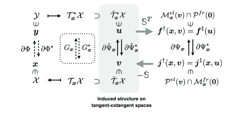
Figure 7: The induced dually flat structure on the restricted tangent and cotangent spaces from the dissipation functions on the edge spaces (gray region). The relationship is compared with the Riemannian metric on tangent and cotangent spaces via Fisher information matrices induced by the thermodynamic functions (dotted box).

Lemma 4 (Equilibrium force as the minimizer of primal dissipation function).

For a given trajectory $\{\bm{x}_{t}\}$, we define the trajectory of the flux $\{\bm{j}^{\dagger}_{t}\}$ minimizing the primal dissipation:

$$\{\bm{j}^{\dagger}_{t}\}:=\arg\min_{\{\bm{j}_{t}\}}\int_{0}^{t}\Psi_{\bm{x}_{t^{\prime}}}[\bm{j}_{t^{\prime}}]\mathrm{d}t^{\prime},\quad\mbox{s.t. $\dot{\bm{x}}_{t^{\prime}}+\mathrm{div}_{\mathbb{S}}\bm{j}_{t^{\prime}}=0$ for all $t^{\prime}\in[0,t]$}.$$ (128)

Then, $\bm{j}^{\dagger}_{t}$ is generated by the equilibrium force, $\bm{f}_{t}^{\dagger}=\partial\Psi_{\bm{x}}[\bm{j}^{\dagger}_{t}]\in\mathcal{P}^{fr}(\bm{0})$. Thus, the minimum primal dissipation flux that generates the given $\{\bm{x}_{t}\}$ is the equilibrium flux.

Proof.

Because the minimization of Eq. 128 can be conducted pointwise-manner for each $t^{\prime}\in[0,t]$ and $\dot{\bm{x}}_{t^{\prime}}+\mathrm{div}_{\mathbb{S}}\bm{j}_{t^{\prime}}=0\Longleftrightarrow\bm{j}_{t^{\prime}}\in\mathcal{P}^{vl}(\dot{\bm{x}}_{t^{\prime}})$, we have

$$\bm{j}_{t^{\prime}}^{\dagger}=\bm{j}^{\dagger}(\bm{x}_{t^{\prime}},\dot{\bm{x}}_{t^{\prime}})=\arg\min_{\bm{j}\in\mathcal{P}^{vl}(\dot{\bm{x}}_{t^{\prime}})}\Psi_{\bm{x}_{t^{\prime}}}[\bm{j}]=\mathcal{P}^{vl}(\dot{\bm{x}}_{t^{\prime}})\cap\mathcal{M}^{fr}_{\bm{x}_{t^{\prime}}}(\bm{0}),$$ (129)

where we used Eq. 115 and Eq. 116. Thus, from $\bm{j}_{t^{\prime}}^{\dagger}\in\mathcal{M}^{fr}_{\bm{x}_{t^{\prime}}}(\bm{0})\Longleftrightarrow\bm{f}_{t^{\prime}}^{\dagger}\in\mathcal{P}^{fr}(\bm{0})$, the minimum dissipation flux $\{\bm{j}^{\dagger}_{t}\}$ is generated by the equilibrium force, $\{\bm{f}_{t}^{\dagger}\}=\{\bm{f}^{\dagger}(\bm{x}_{t^{\prime}},\dot{\bm{x}}_{t^{\prime}})\}\in\mathcal{P}^{fr}(\bm{0})$ where $\bm{f}^{\dagger}(\bm{x},\dot{\bm{x}}):=\partial\Psi_{\bm{x}}[\bm{j}^{\dagger}(\bm{x},\dot{\bm{x}})]$. ∎

By exploiting this unique pairing between $\dot{\bm{x}}_{t^{\prime}}$ and $\bm{j}_{t^{\prime}}^{\dagger}$ or $\dot{\bm{x}}_{t^{\prime}}$ and $\bm{f}_{t^{\prime}}^{\dagger}$, we can obtain an induced dually flat structure on the restricted tangent and cotangent spaces of $\mathcal{X}$ and $\mathcal{Y}$ (Fig. 7), which can be regarded as an information-geometric extension of the Otto structure.

Theorem 2 (Induced dually flat structure on tangent and cotangent spaces).

Let $\tilde{\mathcal{T}}_{\bm{x}}\mathcal{X}:=\mathrm{Im}\mathbb{S}\cong\mathcal{P}^{sc}(\bm{0})\subset\mathcal{T}_{\bm{x}}\mathcal{X}$ and $\tilde{\mathcal{T}}_{\bm{x}}^{*}\mathcal{X}:=\mathcal{T}_{\bm{x}}^{*}\mathcal{X}/\mathrm{Ker}\mathbb{S}^{T}$ be tangent and cotangent spaces on $\mathcal{X}$ restricted by $\mathbb{S}$. On $\tilde{\mathcal{T}}_{\bm{x}}\mathcal{X}$ and $\tilde{\mathcal{T}}_{\bm{x}}^{*}\mathcal{X}$, we have the Legendre conjugate dissipation functions $\tilde{\Psi}_{\bm{x}}:\tilde{\mathcal{T}}_{\bm{x}}\mathcal{X}\to\mathbb{R}$ and $\tilde{\Psi}_{\bm{x}}^{*}:\tilde{\mathcal{T}}_{\bm{x}}^{*}\mathcal{X}\to\mathbb{R}$ induced by the dissipation functions on the edge spaces (Fig. 7).

Proof.

By employing Eq. 129, for each $\bm{v}\in\tilde{\mathcal{T}}_{\bm{x}}\mathcal{X}$, we can uniquely determine $\bm{j}^{\dagger}(\bm{x},\bm{v})$, $\bm{f}^{\dagger}(\bm{x},\bm{v})\in\mathcal{P}^{fr}(\bm{0})$, and $\bm{u}^{\dagger}(\bm{x},\bm{v})\in\tilde{\mathcal{T}}_{\bm{x}}^{*}\mathcal{X}$. They satisfy

$$\bm{v} =-\mathbb{S}\bm{j}^{\dagger}(\bm{x},\bm{v}), \bm{j}^{\dagger}(\bm{x},\bm{v}) =\partial\Psi^{*}_{\bm{x}}[\bm{f}^{\dagger}(\bm{x},\bm{v})], \bm{f}^{\dagger}(\bm{x},\bm{v}) =-\mathbb{S}^{T}\bm{u}^{\dagger}(\bm{x},\bm{v}).$$ (130)

Conversely, for a given $\bm{u}\in\tilde{\mathcal{T}}_{\bm{x}}^{*}\mathcal{X}$, we have $\bm{f}^{\ddagger}(\bm{u})$, $\bm{j}^{\ddagger}(\bm{x},\bm{u})$, and $\bm{v}^{\ddagger}(\bm{x},\bm{u})$ as follows:

$$\bm{v}^{\ddagger}(\bm{x},\bm{u}) =-\mathbb{S}\bm{j}^{\ddagger}(\bm{x},\bm{u}), \bm{j}^{\ddagger}(\bm{x},\bm{u}) =\partial\Psi^{*}_{\bm{x}}[\bm{f}^{\ddagger}(\bm{u})], \bm{f}^{\ddagger}(\bm{u}) =-\mathbb{S}^{T}\bm{u}.$$ (131)

Thus, for a pair of $(\bm{v},\bm{u})_{\bm{x}}$ satisfying $\bm{u}=\bm{u}^{\dagger}(\bm{x},\bm{v})$, we have $\bm{v}=\bm{v}^{\ddagger}(\bm{x},\bm{u})$, $\bm{j}^{\dagger}(\bm{x},\bm{v})=\bm{j}^{\ddagger}(\bm{x},\bm{u})$, and $\bm{f}^{\dagger}(\bm{x},\bm{v})=\bm{f}^{\ddagger}(\bm{x},\bm{u})$. This pairing establishes a bijection between $\tilde{\mathcal{T}}_{\bm{x}}\mathcal{X}$ and $\tilde{\mathcal{T}}_{\bm{x}}^{*}\mathcal{X}$. Moreover, this bijection is realized by the Legendre transformations of the following induced dissipation functions on $\tilde{\mathcal{T}}_{\bm{x}}\mathcal{X}$ and $\tilde{\mathcal{T}}_{\bm{x}}^{*}\mathcal{X}$:

$$\tilde{\Psi}_{\bm{x}}(\bm{v}) :=\Psi_{\bm{x}}(\bm{j}^{\dagger}(\bm{x},\bm{v})), \tilde{\Psi}_{\bm{x}}^{*}(\bm{u}) :=\Psi_{\bm{x}}^{*}(\bm{f}^{\ddagger}(\bm{u})).$$ (132)

These functions are Legendre conjugate as follows:

$$\max_{\bm{u}^{\prime}\in\tilde{\mathcal{T}}^{*}_{\bm{x}}\mathcal{X}} \left[\langle\bm{v},\bm{u}^{\prime}\rangle-\tilde{\Psi}_{\bm{x}}^{*}(\bm{u}^{\prime})\right]=\max_{\begin{subarray}{c}\bm{u}^{\prime}\in\tilde{\mathcal{T}}^{*}_{\bm{x}}\mathcal{X}\\ \bm{j}\in\mathcal{P}^{vl}(\bm{v})\end{subarray}}\left[\langle-\mathbb{S}\bm{j},\bm{u}^{\prime}\rangle-\tilde{\Psi}_{\bm{x}}^{*}(\bm{u}^{\prime})\right]=\max_{\begin{subarray}{c}\bm{u}^{\prime}\in\tilde{\mathcal{T}}^{*}_{\bm{x}}\mathcal{X}\\ \bm{j}\in\mathcal{P}^{vl}(\bm{v})\end{subarray}}\left[\langle\bm{j},-\mathbb{S}^{T}\bm{u}^{\prime}\rangle-\Psi_{\bm{x}}^{*}(-\mathbb{S}^{T}\bm{u}^{\prime})\right]$$

$$=\max_{\begin{subarray}{c}\bm{f}^{\prime}\in\mathcal{P}^{fr}(\bm{0})\\ \bm{j}\in\mathcal{P}^{vl}(\bm{v})\end{subarray}}\left[\langle\bm{j},\bm{f}^{\prime}\rangle-\Psi_{\bm{x}}^{*}(\bm{f}^{\prime})\right]=\max_{\begin{subarray}{c}\bm{f}^{\prime}\in\mathcal{P}^{fr}(\bm{0})\\ \bm{j}\in\mathcal{P}^{vl}(\bm{v})\end{subarray}}\left[\langle\bm{j}^{\dagger}(\bm{x},\bm{v}),\bm{f}^{\prime}\rangle-\Psi_{\bm{x}}^{*}(\bm{f}^{\prime})+\langle(\bm{j}-\bm{j}^{\dagger}(\bm{x},\bm{v})),\bm{f}^{\prime}\rangle\right]$$

$$=\max_{\begin{subarray}{c}\bm{f}^{\prime}\in\mathcal{P}^{fr}(\bm{0})\end{subarray}}\left[\langle\bm{j}^{\dagger}(\bm{x},\bm{v}),\bm{f}^{\prime}\rangle-\Psi_{\bm{x}}^{*}(\bm{f}^{\prime})\right]=\Psi_{\bm{x}}(\bm{j}^{\dagger}(\bm{x},\bm{v}))=\tilde{\Psi}_{\bm{x}}(\bm{v}),$$

where we used $\langle\bm{j}-\bm{j}^{\dagger}(\bm{x},\bm{v}),\bm{f}^{\prime}\rangle=0$ because $\bm{f}^{\prime}\in\mathcal{P}^{fr}(\bm{0})=\mathrm{Im}\mathbb{S}^{T}$ and $(\bm{j}-\bm{j}^{\dagger}(\bm{x},\bm{v}))\in\mathrm{Ker}\mathbb{S}$. The inverse is also shown:

$$\max_{\bm{v}^{\prime}\in\tilde{\mathcal{T}}_{\bm{x}}\mathcal{X}} \left[\langle\bm{v}^{\prime},\bm{u}\rangle-\tilde{\Psi}_{\bm{x}}(\bm{v}^{\prime})\right]=\max_{\begin{subarray}{c}\bm{v}^{\prime}\in\tilde{\mathcal{T}}_{\bm{x}}\mathcal{X}\end{subarray}}\left[\langle-\mathbb{S}\bm{j}^{\dagger}(\bm{x},\bm{v}^{\prime}),\bm{u}\rangle-\Psi_{\bm{x}}(\bm{j}^{\dagger}(\bm{x},\bm{v}^{\prime}))\right]$$

$$=\max_{\begin{subarray}{c}\bm{j}^{\dagger}\in\mathcal{M}^{fr}_{\bm{x}}(\bm{0})\end{subarray}}\left[\langle\bm{j}^{\dagger},-\mathbb{S}^{T}\bm{u}\rangle-\Psi_{\bm{x}}(\bm{j}^{\dagger})\right]=\max_{\bm{j}^{\dagger}\in\mathcal{M}^{fr}_{\bm{x}}(\bm{0})}\left[\langle\bm{j}^{\dagger},\bm{f}^{\ddagger}(\bm{u})\rangle-\Psi_{\bm{x}}(\bm{j}^{\dagger})\right]$$

$$=\Psi_{\bm{x}}^{*}(\bm{f}^{\ddagger}(\bm{u}))=\tilde{\Psi}_{\bm{x}}^{*}(\bm{u}),$$

where we used the fact that $\{\bm{j}^{\dagger}(\bm{x},\bm{v}^{\prime})\}_{\bm{v}^{\prime}\in\tilde{\mathcal{T}}_{\bm{x}}\mathcal{X}}=\mathcal{M}^{fr}_{\bm{x}}(\bm{0})$ in the second line. The pair $(\bm{v}$, $\bm{u})_{\bm{x}}$ are Legendre dual of these functions:

$$\partial_{\bm{v}}\tilde{\Psi}_{\bm{x}}(\bm{v}) =\left[\frac{\partial\bm{j}^{\dagger}(\bm{x},\bm{v})}{\partial\bm{v}}\right]^{T}\left.\frac{\partial\Psi_{\bm{x}}(\bm{j})}{\partial\bm{j}}\right|_{\bm{j}=\bm{j}^{\dagger}(\bm{x},\bm{v})}=\left[\frac{\partial\bm{j}^{\dagger}(\bm{x},\bm{v})}{\partial\bm{v}}\right]^{T}\bm{f}^{\dagger}(\bm{x},\bm{v})$$ (133)

$$=-\left[\frac{\partial\bm{j}^{\dagger}(\bm{x},\bm{v})}{\partial\bm{v}}\right]^{T}\mathbb{S}^{T}\bm{u}^{\dagger}(\bm{x},\bm{v})=\bm{u},$$ (134)

$$\partial_{\bm{u}}\tilde{\Psi}^{*}_{\bm{x}}(\bm{u}) =\left[\frac{\partial\bm{f}^{\ddagger}(\bm{u})}{\partial\bm{u}}\right]^{T}\left.\frac{\partial\Psi^{*}_{\bm{x}}(\bm{f})}{\partial\bm{f}}\right|_{\bm{f}=\bm{f}^{\ddagger}(\bm{u})}=\left[\frac{\partial\bm{f}^{\ddagger}(\bm{u})}{\partial\bm{u}}\right]^{T}\bm{j}^{\ddagger}(\bm{x},\bm{u})$$ (135)

$$=-\mathbb{S}\bm{j}^{\ddagger}(\bm{x},\bm{u})=\bm{v},$$ (136)

where we used $\left[\frac{\partial\bm{j}^{\dagger}(\bm{x},\bm{v})}{\partial\bm{v}}\right]^{T}\mathbb{S}^{T}=-I$ from $\frac{\partial}{\partial\bm{v}}[\bm{v}+\mathbb{S}\bm{j}^{\dagger}(\bm{x},\bm{v})]=I+\mathbb{S}\frac{\partial\bm{j}^{\dagger}(\bm{x},\bm{v})}{\partial\bm{v}}=0$ and $\frac{\partial\bm{f}^{\ddagger}(\bm{u})}{\partial\bm{u}}=-\mathbb{S}^{T}$. They are dissipation functions; strict convexity and $1$-coercivity follow from those of the original dissipation functions. Also, we have

Symmetry $$\tilde{\Psi}_{\bm{x}}(-\bm{v}) =\Psi_{\bm{x}}(\bm{j}^{\dagger}(\bm{x},-\bm{v}))=\Psi_{\bm{x}}(-\bm{j}^{\dagger}(\bm{x},\bm{v}))=\tilde{\Psi}_{\bm{x}}(\bm{v})$$ (137)

Bounded by $0$ at $\bm{0}$ $\displaystyle\tilde{\Psi}_{\bm{x}}(\bm{v}=\bm{0})$ $\displaystyle=\Psi_{\bm{x}}(\bm{j}^{\dagger}(\bm{x},\bm{0}))=\Psi_{\bm{x}}(\bm{0})=0.$ (138)

∎

Using the induced dissipation functions, we define the Bregman divergence on $(\tilde{\mathcal{T}}_{\bm{x}}\mathcal{X},\tilde{\mathcal{T}}^{*}_{\bm{x}}\mathcal{X})$, which is associated with the Bregman divergence on $(\mathcal{J}_{\bm{x}},\mathcal{F}_{\bm{x}})$:

$$\mathcal{D}^{\mathcal{X},\mathcal{Y}}_{\tilde{\Psi}_{\bm{x}}}[\bm{v}\|\bm{u}^{\prime}] :=\tilde{\Psi}_{\bm{x}}(\bm{v})+\tilde{\Psi}_{\bm{x}}^{*}(\bm{u}^{\prime})-\langle\bm{v},\bm{u}^{\prime}\rangle$$ (139)

$$=\Psi_{\bm{x}}(\bm{j}^{\dagger})+\Psi_{\bm{x}}^{*}(\bm{f}^{\prime\ddagger})-\langle\bm{j}^{\dagger},\bm{f}^{\prime\ddagger}\rangle=\mathcal{D}^{\mathcal{J},\mathcal{F}}_{\bm{x}}[\bm{j}^{\dagger}\|\bm{f}^{\prime\ddagger}],$$ (140)

where $\bm{j}^{\dagger}=\bm{j}^{\dagger}(\bm{x},\bm{v})$ and $\bm{f}^{\prime\ddagger}=\bm{f}^{\ddagger}(\bm{x},\bm{u}^{\prime})$. Therefore, we have the induced dually flat structure on $(\tilde{\mathcal{T}}_{\bm{x}}\mathcal{X},\tilde{\mathcal{T}}_{\bm{x}}^{*}\mathcal{X})$. This induced structure can be regarded as an extension to discrete manifolds of the Otto structure [65, 66]: the formal Riemannian structure induced by the $L^{2}$ -Wasserstein distance. This is also related to Pistone’s infinite-dimensional information geometry[125, 72].

VIII.3 Fisher information, natural gradient, mirror descent, evolutionary computation, and optimal transport

In information geometry, it is conventional to use the Fisher information matrices, i.e., the Hessian matrices $G_{\bm{x}}$ and $G^{*}_{\bm{y}}$ (Eq. 31) as the metric tensor (Fisher–Rao metric) on $(\mathcal{T}_{\bm{x}}\mathcal{X},\mathcal{T}_{\bm{x}}^{*}\mathcal{X})$ or equivalently on $(\mathcal{T}_{\bm{y}}\mathcal{Y},\mathcal{T}_{\bm{y}}^{*}\mathcal{Y})$ (Fig. 7). Gradient systems have been defined information-geometrically[25] as a Riemannian gradient flow using the Bregman divergence and the Fisher information matrix of $\Phi(\bm{x})$ as the gradient function and the metric tensor, respectively: $\dot{\bm{x}}=-G_{\bm{x}}^{-1}\partial\mathcal{D}^{\mathcal{X}}_{\Phi}[\bm{x}\|\tilde{\bm{x}}]$. Because both $G_{\bm{x}}$ and $\mathcal{D}^{\mathcal{X}}_{\Phi}$ are derived from $\Phi(\bm{x})$, this gradient flow becomes a geodesic in $\mathcal{Y}$ space: $\dot{\bm{y}}=-(\bm{y}-\tilde{\bm{y}})$. In natural gradient descent [152, 67, 69], the Fisher information matrix is used to find the steepest descent gradient of a function $\mathcal{F}(\bm{\theta})$ on a parameter space $\Theta$ as $\dot{\bm{\theta}}=-G_{\bm{\theta}}^{-1}\partial\mathcal{F}(\bm{\theta})$, where $G_{\bm{\theta}}$ is determined independently of $\mathcal{F}(\bm{\theta})$ by considering the underlying model parameter space. In optimization, the natural gradient is fundamental in information-geometric optimization algorithms, which contain various evolutionary optimization schemes[70]. In relation to machine learning, the mirror descent is identified with the natural gradient descent by a naive continuous limit[69, 153]. Furthermore, optimal transport has recently been employed to replace or integrate the Fisher-Rao metric with the Wasserstein metrics[154, 155]. Because the Wasserstein metric can take the information of the base manifold into account, their integration may provide more amenable ways to accommodate various prior and structural information.

The doubly dual flat structure introduced in this work actually provides a solution to generalize those results and the associated problems. The base space $\mathcal{X}$ with the dually flat structure and the associated Fisher information matrix accommodates the conventional natural gradient. The graph or hypergraph structure endows the additional topological relation to the base space of $\mathcal{X}$. The dissipation functions on the edge spaces or their induced versions bestow a more flexible way than the Fisher-Rao metric to represent the loss of the potential function, i.e., the dissipation, at each point in the state space. Upon necessity, we may combine both of them (Fig. 7), for example, as $\dot{\bm{x}}=-G_{\bm{x}}^{-1}\partial\mathcal{F}^{(1)}(\bm{x})-\mathrm{div}_{\mathbb{S}}\partial\Psi^{*}_{\bm{x}}[\mathrm{grad}_{\mathbb{S}}\partial\mathcal{F}^{(2)}(\bm{x})]$ where $\mathcal{F}^{(1)}(\bm{x})$ and $\mathcal{F}^{(2)}(\bm{x})$ could be different. This flexibility may contribute to the design of new algorithms for machine learning. Actually, this integrated representation is quite relevant to the filtering equations[156] in sequential inference where the first term, i.e., $-G_{\bm{x}}^{-1}\partial\mathcal{F}^{(1)}(\bm{x})$, can usually be associated with the update of posterior probability by observation and the second term, $-\mathrm{div}_{\mathbb{S}}\partial\Psi^{*}_{\bm{x}}[\mathrm{grad}_{\mathbb{S}}\partial\mathcal{F}^{(2)}(\bm{x})]$ can represent the prediction by the prior information on the dynamics. Our framework may provide a unified information-geometric perspective to various information-geometric analyses and extensions of filtering, e.g., projection-filters[157], information-geometric nonlinear filtering[158], and information geometric optimization[70] Furthermore, the generalized gradient flow can be regarded as a continuous time limit of the mirror descent where the nonlinear Legendre duality between primal and dual spaces is preserved at the limit. This fact may be employed to design new gradient-based algorithms based on the doubly dual flat structure.

IX Information-geometric Properties of Generalized Nonequilibrium Flow

In this section, we consider the nonequilibrium flow defined by Eq. 61, i.e.,

$$\dot{\bm{x}}=-\mathrm{div}_{\mathbb{S}}\partial\Psi^{*}_{\bm{x}}\left[\left[\mathrm{grad}_{\mathbb{S}}\partial\mathcal{D}^{\mathcal{X}}_{\Phi}[\bm{x}\|\tilde{\bm{x}}]\right]+\bm{f}_{NE}\right],$$ (141)

with $\bm{f}_{NE}\not\in\mathrm{Im}\mathbb{S}^{T}$, and show how information geometry can be employed to analyze such dynamics. While we can obtain several properties of equilibrium flow independently of the detail of the thermodynamic function and the dissipation function, these functions should be related so as to obtain nice properties for the nonequilibrium flow. We will observe that the thermodynamic function and the dissipation function of LMA kinetics actually have such a relation.

IX.1 Gradient-flow-like property and Lyapunov function of nonequilibrium flow

For the equilibrium flow (Eq. 58), the Bregman divergence $\mathcal{D}^{\mathcal{X}}_{\Phi}[\bm{x}\|\tilde{\bm{x}}]$ is a Lyapunov function. The Bregman divergence can still be a Lyapunov function even for the nonequilibrium flow (Eq. 141) under the following conditions:

Lemma 5.

Suppose that, for all $\bm{x}\in\mathcal{X}$, the force $\bm{f}(\bm{x})=\mathrm{grad}_{\mathbb{S}}\partial\mathcal{D}^{\mathcal{X}}_{\Phi}[\bm{x}\|\tilde{\bm{x}}]+\bm{f}_{NE}$ is orthogonally decomposed as $\bm{f}(\bm{x})=\bm{f}_{S}(\bm{x})+\bm{f}_{A}(\bm{x})$ where $\bm{f}_{S}(\bm{x}):=\mathrm{grad}_{\mathbb{S}}\partial_{\bm{x}}\mathcal{D}^{\mathcal{X}}_{\Phi}[\bm{x}\|\tilde{\bm{x}}_{CB}]$ and $\bm{f}_{A}(\bm{x})\in\mathcal{F}_{\bm{x}}$ satisfy the pseudo-Hilbert-isosceles orthogonality $\bm{f}_{S}(\bm{x})\perp_{H}\bm{f}_{A}(\bm{x})$. Then $\frac{\mathrm{d}}{\mathrm{d}t}\mathcal{D}^{\mathcal{X}}_{\Phi}[\bm{x}_{t}\|\tilde{\bm{x}}_{CB}]\leq 0$ holds. In addition, $\bm{x}_{CB}=\mathcal{P}^{sc}(\bm{x}_{0})\cap\mathcal{M}^{eq}(\tilde{\bm{x}}_{CB})$ is the unique steady state of Eq. 141 with the initial state $\bm{x}_{0}$ that attains $\frac{\mathrm{d}}{\mathrm{d}t}\mathcal{D}^{\mathcal{X}}_{\Phi}[\bm{x}_{t}\|\tilde{\bm{x}}_{CB}]=0$ . Thus, $\bm{x}_{CB}$ is locally and asymptotically stable.

Proof.

We can directly verify $\frac{\mathrm{d}}{\mathrm{d}t}\mathcal{D}^{\mathcal{X}}_{\Phi}[\bm{x}_{t}\|\tilde{\bm{x}}_{CB}]\leq 0$ as follows:

$$\frac{\mathrm{d}}{\mathrm{d}t}\mathcal{D}^{\mathcal{X}}_{\Phi}[\bm{x}_{t}\|\tilde{\bm{x}}_{CB}] =\langle\dot{\bm{x}},\partial_{\bm{x}}\mathcal{D}^{\mathcal{X}}_{\Phi}[\bm{x}_{t}\|\tilde{\bm{x}}_{CB}]\rangle=-\langle\mathrm{div}_{\mathbb{S}}\bm{j}(\bm{x}),\partial_{\bm{x}}\mathcal{D}^{\mathcal{X}}_{\Phi}[\bm{x}_{t}\|\tilde{\bm{x}}_{CB}]\rangle$$ (142)

$$=-\langle\bm{j}(\bm{x}),\mathrm{grad}_{\mathbb{S}}\partial_{\bm{x}}\mathcal{D}^{\mathcal{X}}_{\Phi}[\bm{x}_{t}\|\tilde{\bm{x}}_{CB}]\rangle$$

$$=-\langle\bm{j}(\bm{x}),\bm{f}_{S}(\bm{x})\rangle=-\frac{1}{2}\mathcal{D}^{\mathcal{J},\mathcal{F}}_{\bm{x}}[\bm{j}(\bm{x})\|-\bm{f}^{\prime\prime}(\bm{x})]\leq 0$$ (143)

where we used Eq. 125 and $\bm{f}^{\prime\prime}(\bm{x}):=\bm{f}_{S}(\bm{x})-\bm{f}_{A}(\bm{x})$. The equality holds if and only if $\bm{f}(\bm{x})=-\bm{f}^{\prime\prime}(\bm{x})$, which means that

$$\bm{f}(\bm{x})=-\bm{f}^{\prime\prime}(\bm{x})\Longleftrightarrow\bm{f}_{S}(\bm{x})=0\Longleftrightarrow\mathrm{grad}_{\mathbb{S}}\partial_{\bm{x}}\mathcal{D}^{\mathcal{X}}_{\Phi}[\bm{x}\|\tilde{\bm{x}}_{CB}]=0\Longleftrightarrow\bm{x}\in\mathcal{M}^{eq}(\tilde{\bm{x}}_{CB}).$$ (144)

Because $\bm{x}_{t}\in\mathcal{P}^{sc}(\bm{x}_{0})$, $\bm{x}_{CB}=\mathcal{P}^{sc}(\bm{x}_{0})\cap\mathcal{M}^{eq}(\tilde{\bm{x}}_{CB})$ holds. ∎

Thus, if the pseudo-Hilbert-isosceles orthogonal decomposition exists, then the nonequilibrium flow behaves like the equilibrium flow.

IX.2 Complex-balanced state and pseudo-Hilbert-isosceles orthogonality

More specific conditions or situations under which the orthogonal decomposition in Lemma 5 exists is still an open problem. However, for CRN with LMA kinetics, the decomposition holds if a complex-balanced steady state exists.

Proposition 9 (Complex-balanced steady state and orthogonal decomposition for CRN with LMA kinetics[78, 81, 79, 83]).

Suppose that a complex balanced steady state exists, i.e., $\mathcal{M}^{\mathrm{CB}}\neq\emptyset$ for CRN with LMA kinetics (Eq. 12). Using any $\tilde{\bm{x}}_{CB}\in\mathcal{M}^{\mathrm{CB}}$, consider a decomposition of the force $\bm{f}_{MA}(\bm{x})$ as $\bm{f}_{MA}(\bm{x})=\bm{f}_{S}(\bm{x})+\bm{f}_{A}$ where $\bm{f}_{S}(\bm{x})=\mathrm{grad}_{\mathbb{S}}\partial_{\bm{x}}\mathcal{D}^{\mathcal{X}}_{\Phi}[\bm{x}\|\tilde{\bm{x}}_{CB}]$, $\bm{f}_{A}=\ln\bm{K}+\mathbb{S}^{T}\ln\tilde{\bm{x}}_{CB}$, and $\Phi(\bm{x})$ is as in Eq. 62. Then, for the dissipation functions in Eq. 68, the pseudo-Hilbert isosceles orthogonality $\bm{f}_{S}(\bm{x})\perp_{H}\bm{f}_{A}$ holds for all $\bm{x}\in\mathcal{X}$. In addition, $\mathcal{M}^{eq}(\tilde{\bm{x}}_{CB})=\mathcal{M}^{\mathrm{CB}}$ holds.

Proof.

We can prove the orthogonality by direct computation. The orthogonality condition is

$$\Psi^{*}_{\bm{x}}[\bm{f}_{S}(\bm{x})+\bm{f}_{A}] =\Psi^{*}_{\bm{x}}[\bm{f}_{S}(\bm{x})-\bm{f}_{A}]$$ (145)

$$\Leftrightarrow\left\langle\bm{j}^{+}_{MA}(\bm{x}),\left(\frac{\bm{x}}{\tilde{\bm{x}}_{CB}}\right)^{-\mathbb{S}^{T}}-\bm{1}\right\rangle+\left\langle\bm{j}^{-}_{MA}(\bm{x}),\left(\frac{\bm{x}}{\tilde{\bm{x}}_{CB}}\right)^{\mathbb{S}^{T}}-\bm{1}\right\rangle=0.$$ (146)

Consider the following equality:

$$\left\langle\bm{j}^{\pm}_{MA}(\bm{x}),\left(\frac{\bm{x}}{\tilde{\bm{x}}_{CB}}\right)^{\mp\mathbb{S}^{T}}-\bm{1}\right\rangle =\sum_{e=1}^{N_{\mathbb{e}}}k_{e}^{\pm}\tilde{\bm{x}}_{CB}^{\bm{\gamma}_{e}^{\pm}}\left[\left(\frac{\bm{x}}{\tilde{\bm{x}}_{CB}}\right)^{\bm{\gamma}_{e}^{\mp}}-\left(\frac{\bm{x}}{\tilde{\bm{x}}_{CB}}\right)^{\bm{\gamma}_{e}^{\pm}}\right],$$ (147)

where $\bm{\gamma}_{e}^{\pm}:={\mathchoice{\raisebox{0.0pt}{\scalebox{1.0}[-1.0]{$\displaystyle\mathbb{L}$}}}{\raisebox{0.0pt}{\scalebox{1.0}[-1.0]{$\textstyle\mathbb{L}$}}}{\raisebox{0.0pt}{\scalebox{1.0}[-1.0]{$\scriptstyle\mathbb{L}$}}}{\raisebox{0.0pt}{\scalebox{1.0}[-1.0]{$\scriptscriptstyle\mathbb{L}$}}}}\bm{b}_{e}^{\pm}$. By using this, we have the following:

Eq. 146 $$=\sum_{e=1}^{N_{\mathbb{e}}}\left(k_{e}^{+}\tilde{\bm{x}}_{CB}^{\gamma_{e}^{+}}-k_{e}^{-}\tilde{\bm{x}}_{CB}^{\gamma_{e}^{-}}\right)\left[\left(\frac{\bm{x}}{\tilde{\bm{x}}_{CB}}\right)^{\gamma_{e}^{-}}-\left(\frac{\bm{x}}{\tilde{\bm{x}}_{CB}}\right)^{\gamma_{e}^{+}}\right]$$ (148)

$$=\left\langle(\bm{j}^{+}_{MA}(\tilde{\bm{x}}_{CB})-\bm{j}^{-}_{MA}(\tilde{\bm{x}}_{CB})),\left[\left(\frac{\bm{x}}{\tilde{\bm{x}}_{CB}}\right)^{({\mathchoice{\raisebox{0.0pt}{\scalebox{1.0}[-1.0]{$\displaystyle\mathbb{L}$}}}{\raisebox{0.0pt}{\scalebox{1.0}[-1.0]{$\textstyle\mathbb{L}$}}}{\raisebox{0.0pt}{\scalebox{1.0}[-1.0]{$\scriptstyle\mathbb{L}$}}}{\raisebox{0.0pt}{\scalebox{1.0}[-1.0]{$\scriptscriptstyle\mathbb{L}$}}}}\mathbb{B}^{-})^{T}}-\left(\frac{\bm{x}}{\tilde{\bm{x}}_{CB}}\right)^{({\mathchoice{\raisebox{0.0pt}{\scalebox{1.0}[-1.0]{$\displaystyle\mathbb{L}$}}}{\raisebox{0.0pt}{\scalebox{1.0}[-1.0]{$\textstyle\mathbb{L}$}}}{\raisebox{0.0pt}{\scalebox{1.0}[-1.0]{$\scriptstyle\mathbb{L}$}}}{\raisebox{0.0pt}{\scalebox{1.0}[-1.0]{$\scriptscriptstyle\mathbb{L}$}}}}\mathbb{B}^{+})^{T}}\right]\right\rangle$$ (149)

$$=\left\langle\bm{j}_{MA}(\tilde{\bm{x}}_{CB}),\mathbb{B}^{T}_{-}\left(\frac{\bm{x}}{\tilde{\bm{x}}_{CB}}\right)^{{\mathchoice{\raisebox{0.0pt}{\scalebox{1.0}[-1.0]{$\displaystyle\mathbb{L}$}}}{\raisebox{0.0pt}{\scalebox{1.0}[-1.0]{$\textstyle\mathbb{L}$}}}{\raisebox{0.0pt}{\scalebox{1.0}[-1.0]{$\scriptstyle\mathbb{L}$}}}{\raisebox{0.0pt}{\scalebox{1.0}[-1.0]{$\scriptscriptstyle\mathbb{L}$}}}}^{T}}-\mathbb{B}^{T}_{+}\left(\frac{\bm{x}}{\tilde{\bm{x}}_{CB}}\right)^{{\mathchoice{\raisebox{0.0pt}{\scalebox{1.0}[-1.0]{$\displaystyle\mathbb{L}$}}}{\raisebox{0.0pt}{\scalebox{1.0}[-1.0]{$\textstyle\mathbb{L}$}}}{\raisebox{0.0pt}{\scalebox{1.0}[-1.0]{$\scriptstyle\mathbb{L}$}}}{\raisebox{0.0pt}{\scalebox{1.0}[-1.0]{$\scriptscriptstyle\mathbb{L}$}}}}^{T}}\right\rangle=\left\langle\mathbb{B}\bm{j}_{MA}(\tilde{\bm{x}}_{CB}),\left(\frac{\bm{x}}{\tilde{\bm{x}}_{CB}}\right)^{{\mathchoice{\raisebox{0.0pt}{\scalebox{1.0}[-1.0]{$\displaystyle\mathbb{L}$}}}{\raisebox{0.0pt}{\scalebox{1.0}[-1.0]{$\textstyle\mathbb{L}$}}}{\raisebox{0.0pt}{\scalebox{1.0}[-1.0]{$\scriptstyle\mathbb{L}$}}}{\raisebox{0.0pt}{\scalebox{1.0}[-1.0]{$\scriptscriptstyle\mathbb{L}$}}}}^{T}}\right\rangle.$$ (150)

Thus, Eq. 145 holds for $\bm{x}\in\mathcal{X}$ if $\mathbb{B}\bm{j}_{MA}(\tilde{\bm{x}}_{CB})=\bm{0}$ holds. $\mathcal{M}^{eq}(\tilde{\bm{x}}_{CB})=\mathcal{M}^{\mathrm{CB}}$ can be proved by obtaining the parametric representation of $\mathcal{M}^{\mathrm{CB}}$ as $\mathcal{M}^{\mathrm{CB}}=\{\bm{x}\in\mathcal{X}|\ln\bm{x}-\ln\tilde{\bm{x}}_{CB}\in\mathrm{Ker}\mathbb{S}^{T}\}$ via solving $\bm{j}_{MA}(\bm{x})=\bm{0}$. This representation is identical to that of $\mathcal{M}^{eq}(\tilde{\bm{x}}_{CB})$ (Eq. 104). ∎

Remark 10 (Algebraic structure of detailed balanced and complex balanced manifolds).

We here mention about the underlying algebraic source of why $\mathcal{M}^{eq}(\tilde{\bm{x}}_{CB})=\mathcal{M}^{\mathrm{CB}}$ holds. First, we already showed that $\mathcal{M}^{DB}=\mathcal{M}^{eq}(\tilde{\bm{x}})$ holds generally if $\mathcal{M}^{\mathrm{DB}}\neq\emptyset$. Under LMA kinetics (Eq. 12), the DB condition $\bm{j}_{MA}(\bm{x})=\bm{0}$ is nothing but the binomial equations because $\bm{j}^{\pm}_{MA}(\bm{x})$ are vectors of monominals of $\bm{x}$. Owing to this, $\mathcal{M}^{DB}$ becomes a toric variety. In contrast, the CB condition $\mathbb{B}\bm{j}_{MA}(\bm{x}_{CB})=\bm{0}$ is a set of polynomial equations for LMA kinetics. Nonetheless, it was shown that $\mathcal{M}^{\mathrm{CB}}$ is binomially generated and has the same structural matrix $\mathbb{S}^{T}$ as the equilibrium manifold[101] . Because of that, they become equivalent as manifolds.

Because rLDG (Eq. 3) is a subclass of CRN where ${\mathchoice{\raisebox{0.0pt}{\scalebox{1.0}[-1.0]{$\displaystyle\mathbb{L}$}}}{\raisebox{0.0pt}{\scalebox{1.0}[-1.0]{$\textstyle\mathbb{L}$}}}{\raisebox{0.0pt}{\scalebox{1.0}[-1.0]{$\scriptstyle\mathbb{L}$}}}{\raisebox{0.0pt}{\scalebox{1.0}[-1.0]{$\scriptscriptstyle\mathbb{L}$}}}}=I$ and thus $\mathbb{S}=\mathbb{B}$ holds, the complex-balanced condition is always satisfied for rLDG.

Corollary 1 (rLDG is unconditionally complex-balanced[8]).

All the steady states of rLDG are complex-balanced states, i.e., $\mathcal{M}^{\mathrm{ST}}=\mathcal{M}^{\mathrm{CB}}$ independently of the parameter values $\bm{k}^{\pm}$ of the flux (Eq. 3) . Thus, KL divergence (Eq. 64) always works as a Lyapunov function of rLDG.

The properties described in this corollary are well-known for rMJP and are usually obtained by using the Perron-Frobenius theorem for linear operators. The framework of the generalized flow enables us to extend them to the nonlinear regime.

IX.3 Effective fluw of the nonequilibrium flow by the primal information-geometric projection

In general, the nonequilibrium force or flux has redundant degrees of freedom in terms of generating a specific vector field or trajectory $\{\bm{x}_{t}\}$ on the density space. By using the extended HHK projective decomposition (Thm. 1), we can carve out the effective part of the flux for the trajectory $\{\bm{x}_{t}\}$. In addition, we can obtain an effective time-dependent equilibrium flux that mimics the trajectory $\{\bm{x}_{t}\}$:

Lemma 6 (Effective time-dependent equilibrium flux).

Suppose that $\bm{j}(\bm{x})$ is the flux of a generalized flow (Eq. 45), and define the corresponding effective equilibrium flux by $\bm{j}_{eq}(\bm{x})=\partial\Psi^{*}_{\bm{x}}[\mathbb{S}^{T}\bm{u}_{eq}(\bm{x})]$ where $\bm{u}_{eq}(\bm{x}):=\partial\tilde{\Psi}_{\bm{x}}[-\mathbb{S}\bm{j}(\bm{x})]$. Then, $\bm{j}_{eq}(\bm{x})$ induces the same velocity as $\bm{j}(\bm{x})$ does. Furthermore, for a given trajectory $\{\bm{x}_{t}\}$ of $\bm{j}(\bm{x})$, we can construct a time-dependent equilibrium flux $\bm{j}_{eq}(t,\bm{x})$ that can generate the same $\{\bm{x}_{t}\}$ as follows

$$\bm{j}_{eq}(t,\bm{x}) :=\partial\Psi^{*}_{\bm{x}}\left[\mathrm{grad}_{\mathbb{S}}\partial\mathcal{D}^{\mathcal{X}}_{\Phi}[\bm{x}\|\tilde{\bm{x}_{t}}]\right], \tilde{\bm{x}}_{t}:=\partial\Phi^{*}[\partial\Phi(\bm{x}_{t})+\bm{u}_{eq}(\bm{x}_{t})].$$ (151)

Proof.

From Thm. 1, $\bm{j}(\bm{x})$ can be decomposed as $\bm{j}(\bm{x})=\bm{j}_{eq}(\bm{x})+(\bm{j}(\bm{x})-\bm{j}_{eq}(\bm{x}))$. Because $\bm{f}_{eq}(\bm{x})=\partial\Psi_{\bm{x}}^{*}[\bm{j}_{eq}(\bm{x})]\in\mathcal{P}^{fr}(\bm{0})$, there exists $\bm{u}_{eq}(\bm{x})$ satisfying $-\mathbb{S}^{T}\bm{u}_{eq}(\bm{x})=\bm{f}_{eq}(\bm{x})$. By employing the duality introduced in Thm. 2, $\bm{u}_{eq}(\bm{x})$ can be represented as $\bm{u}_{eq}(\bm{x})=\partial\tilde{\Psi}_{\bm{x}}[\bm{v}(\bm{x})]$ where $\bm{v}(\bm{x})=-\mathbb{S}\bm{j}(\bm{x})$. Because $-\mathbb{S}\bm{j}_{eq}(\bm{x})=\bm{v}(\bm{x})$, $\bm{j}_{eq}(\bm{x})$ generates the same dynamics or vector field as $\bm{j}(\bm{x})$ does. By solving $-\bm{u}_{eq}(\bm{x}_{t})=\partial\Phi(\bm{x}_{t})-\partial\Phi(\tilde{\bm{x}}_{t})$, we have Eq. 151. ∎

The effective time-dependent equilibrium flux is obtained more explicitly for CRN with LMA kinetics:

Corollary 2 (Effective equilibrium force and flux of LMA kinetics).

Consider the following quantities of CRN with LMA kinetics:

Flux defined in Eq. 12 $$\bm{j}_{MA}(\bm{x};\bm{k}^{\pm})$$ (152)

Force defined in Eq. 70 $$\bm{f}_{\mathrm{MA}}(\bm{x};\bm{K})$$ (153)

Thermodynamic function defined in Eq. 62 $$\Phi(\bm{x})$$ (154)

Dissipation functions defined in Eq. 68 with Eq. 70 $$\Psi^{*}_{\bm{x},\bm{\kappa}}[\bm{f}]=\Psi^{*}_{\bm{\omega}_{\mathrm{MA}}(\bm{x};\bm{\kappa})}[\bm{f}],$$ (155)

where $\bm{k}^{\pm}=\bm{\kappa}\circ\bm{K}^{\pm 1/2}$ holds. For a trajectory $\{\bm{x}_{t}\}$ generated by $\bm{j}_{MA}(\bm{x};\bm{k}^{\pm})$, the effective time-dependent equilibrium force $\bm{f}_{eq}(t,\bm{x})$ can be described as $\bm{f}_{MA}(\bm{x};\bm{K}_{eq}(t))$ where $\bm{K}_{eq}(t)$ is determined by

$$\bm{K}_{eq}(t) :=\exp\left[-\mathbb{S}^{T}\left(\bm{u}_{eq}(\bm{x}_{t};\bm{\kappa})+\partial\Phi(\bm{x}_{t})\right)\right], \bm{u}_{eq}(\bm{x}_{t};\bm{\kappa}) :=\partial\tilde{\Psi}_{\bm{x}_{t},\bm{\kappa}}[-\mathbb{S}\bm{j}_{MA}(\bm{x}_{t})]$$ (156)

Thus, the effective time-dependent equilibrium flux $\bm{j}_{eq}(t,\bm{x})$ is represented as $\bm{j}_{eq}(t,\bm{x})=\bm{j}_{MA}(\bm{x};\bm{k}^{\pm}_{eq}(t))$ where $\bm{k}^{\pm}_{eq}(t)=\bm{\kappa}\circ\bm{K}^{\pm 1/2}_{eq}(t)$.

This corollary means that the effective time-dependent flux of LMA kinetics is always obtained by a time-dependent modulation of the kinetic parameters $\bm{k}^{\pm}$. More specifically, the modulation of force part $\bm{K}_{eq}(t)$ is sufficient while the activity part $\bm{\kappa}$ is kept constant.

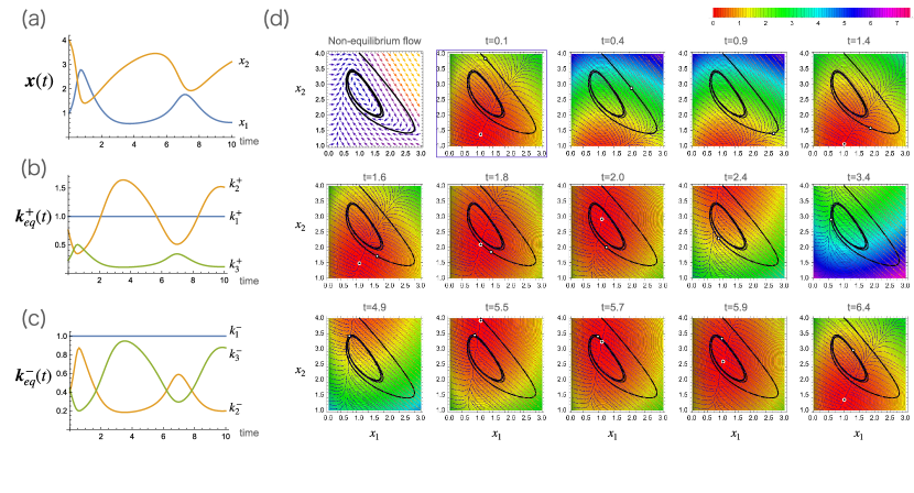
Figure 8: A nonequilibrium trajectory of the Brusselator CRN (Ex. 1) and the associated time-dependent effective equilibrium flux $\bm{j}_{eq}(t,\bm{x})=\bm{j}_{MA}(\bm{x};\bm{k}^{\pm}_{eq}(t))$. (a) A nonequilibrium trajectory $\{\bm{x}_{t}\}$ of the Brusselator CRN for a set of the kinetic parameters, $k_{1}^{+}=1.0$, $k_{1}^{-}=1.0$, $k_{2}^{+}=3.0$, $k_{2}^{-}=0.1$, $k_{3}^{+}=1.0$, $k_{3}^{-}=0.1$, and the initial state $(\bm{x}_{1}(0),\bm{x}_{2}(0))=(1.0,4.0)$. (b,c) The time-dependent kinetic parameter set $\bm{k}^{\pm}_{eq}(t)$, which generates the time-dependent equilibrium flux $\bm{j}_{eq}(t,\bm{x})$. (d) The top left panel shows the nonequilibrium trajectory $\{\bm{x}_{t}\}$ (black curve) and the vector field $\bm{v}(\bm{x})=-\mathbb{S}\bm{j}(\bm{x})$ (arrows). The other panels show the time-dependent vector field $\bm{v}_{eq}(t,\bm{x})$ induced by $\bm{j}_{eq}(t,\bm{x})$: $\bm{v}_{eq}(t,\bm{x})=-\mathbb{S}\bm{j}_{eq}(t,\bm{x})$. The nonequilibrium trajectory $\{\bm{x}_{t}\}$ is also depicted as a reference (the black curve). The color indicates the value of $\mathcal{D}^{\mathcal{X}}_{\Phi}[\bm{x}\|\tilde{\bm{x}_{t}}]$. In each panel, the white circle on the trajectory is $\bm{x}_{t}$ at which $\bm{j}_{eq}(t,\bm{x})$ is computed, and the black circle with a white border corresponds to $\tilde{\bm{x}}_{t}$ at which $\mathcal{D}^{\mathcal{X}}_{\Phi}[\bm{x}\|\tilde{\bm{x}_{t}}]$ is $0$.

Example 3 (Simplified Brusselator CRN[8, 107] (continued)).

By using the Brusselator CRN (Ex. 1), we numerically obtained a nonequilibrium trajectory $\{\bm{x}_{t}\}$ (Fig. 8 (a) and Fig. 8 (d) top left panel). By using Cor. 2, we also computed the corresponding time-dependent kinetic parameter set $\bm{k}^{\pm}_{eq}(t)$ that generates the time-dependent equilibrium flux $\bm{j}_{eq}(t,\bm{x})=\bm{j}_{MA}(t,\bm{x};\bm{k}^{\pm}_{eq}(t))$ (Fig. 8 (b,c)). Figure 8 (d) shows the vector field $\bm{v}_{eq}(t,\bm{x})=-\mathbb{S}\bm{j}_{eq}(t,\bm{x})$ induced by the time-dependent equilibrium flux $\bm{j}_{eq}(t,\bm{x})$ and the contours of $\mathcal{D}^{\mathcal{X}}_{\Phi}[\bm{x}\|\tilde{\bm{x}_{t}}]$ where $\tilde{\bm{x}}_{t}$ follows from Eq. 151. From Fig. 8, we can see that the trajectory $\{\bm{x}_{t}\}$ originally generated by the nonequilibrium flux $\bm{j}(\bm{x})$ can be traced by the time-dependent equilibrium flux $\bm{j}_{eq}(t,\bm{x})$ and also that $\bm{j}_{eq}(t,\bm{x})$ can be physically realized by the modulation of the kinetic parameters $\bm{k}^{\pm}_{eq}(t)$.

IX.4 Characterization of the nonequilibrium flow by the dual information geometric projection

The nonequilibrium flow is redundant in terms of generating a specific vector field or trajectory $\{\bm{x}_{t}\}$. Such redundancy is crucial to characterize the extent of nonequilibrium. One approach for the characterization is to investigate the cycle force or flux, which has been employed in the linear theory of dynamics on graphs and also in graph-theoretic approaches to nonequilibrium phenomena[159, 90, 160, 161, 162]. To extract such cyclic components, we can use $\mathbb{V}^{T}=\mathrm{curl}_{\mathbb{V}}$, its adjoint $\mathbb{V}=\mathrm{curl}^{*}_{\mathbb{V}}$, the associated cycle subspaces $C^{2}(\mathbb{H})$ and $C_{2}(\mathbb{H})$, and also the generalized HKK decomposition (Thm. 1).

Definition 34 (Cycle spaces).

The cycle spaces at $\bm{x}\in\mathcal{X}$ are defined as $\mathcal{Z}_{\bm{x}}=C_{2}(\mathbb{H})=\mathrm{Ker}[\mathbb{V}]$ and $\mathfrak{Z}_{\bm{x}}=C^{2}(\mathbb{H})=\mathrm{Im}[\mathbb{V}^{T}]$.

For a given nonequilibrium force $\bm{f}(\bm{x})$, we can obtain its cycle component $\bm{\zeta}=\mathrm{curl}_{\mathbb{V}}\bm{f}(\bm{x})=\mathbb{V}^{T}\bm{f}(\bm{x})\in\mathfrak{Z}_{\bm{x}}$. $\bm{\zeta}$ contains the information to categorize the force because $\mathcal{P}^{fr}(\bm{f})=\mathcal{P}^{fr}(\bm{\zeta})$ is the quotient space of force by the equilibrium force. For each $\zeta\in\mathfrak{Z}_{\bm{x}}$, we obtain the representative force $\bm{f}^{\lozenge}(\bm{x},\bm{\zeta})$ via the following variational problem:

Lemma 7 (Steady (zero-velocity) force as the minimizer of the dual dissipation function).

For a given $\bm{\zeta}\in\mathfrak{Z}_{\bm{x}}$, we define the force $\bm{f}^{\lozenge}(\bm{x},\bm{\zeta})$ minimizing the dual dissipation function:

$$\bm{f}^{\lozenge}(\bm{x},\bm{\zeta}):=\arg\min_{\bm{f}}\Psi_{\bm{x}}^{*}[\bm{f}],\quad\mbox{s.t. $\mathrm{curl}_{\mathbb{V}}\bm{f}=\bm{\zeta}$}.$$ (157)

Then, $\bm{f}^{\lozenge}(\bm{x},\bm{\zeta})$ is the steady (zero-velocity) force, i.e., $\bm{j}^{\lozenge}=\partial\Psi_{\bm{x}}^{*}[\bm{f}^{\lozenge}]\in\mathcal{P}^{vl}(\bm{0})$.

Proof.

From Eq. 115 in Thm. 1, $\bm{f}^{\lozenge}(\bm{x},\bm{\zeta})\in\mathcal{P}^{fr}(\bm{\zeta})\cap\mathcal{M}^{vl}(\bm{0})$. Thus, $\bm{j}^{\lozenge}\in\mathcal{P}^{vl}(\bm{0})$. ∎

Among various $\bm{f}$ that has the same cyclic component $\bm{\zeta}$, the force $\bm{f}^{\lozenge}(\bm{x},\bm{\zeta})$ is the one that induces no dynamics of $\bm{x}$. Because any dynamics of $\bm{x}$ can be represented by the effective equilibrium flux as in Lemma 6, $\bm{f}^{\lozenge}(\bm{x},\bm{\zeta})$ can be regarded as the force being purely relevant to the cycle.

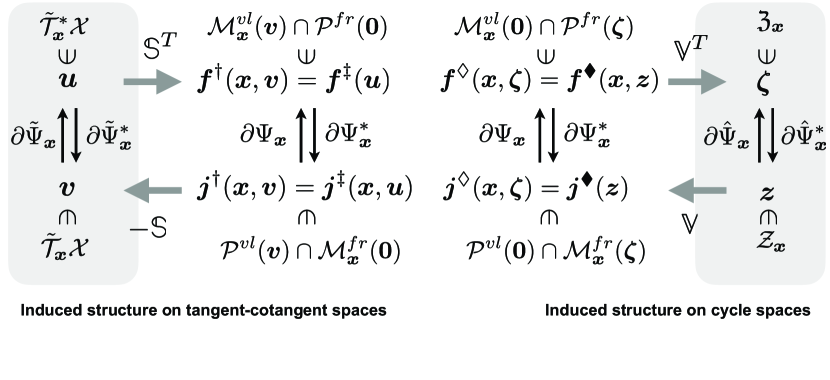
Figure 9: The induced dually flat structure on the cycle spaces (right gray region) in comparison with the induced structure on the restricted tangent and cotangent spaces(left gray region).

Using $\bm{f}^{\lozenge}(\bm{x},\bm{\zeta})$, we can establish the induced duality between $\mathcal{Z}_{\bm{x}}$ and $\mathfrak{Z}_{\bm{x}}$ spaces:

Theorem 3 (Induced dually flat structure on cycle spaces).

On the cycle spaces, $\mathcal{Z}_{\bm{x}}$ and $\mathfrak{Z}_{\bm{x}}$, we have the Legendre conjugate dissipation functions $\hat{\Psi}_{\bm{x}}:\mathcal{Z}_{\bm{x}}\to\mathbb{R}$ and $\hat{\Psi}_{\bm{x}}^{*}:\mathfrak{Z}_{\bm{x}}\to\mathbb{R}$ induced by the dissipation functions on the edge spaces (Fig. 9).

Proof.

For each $\bm{\zeta}\in\mathfrak{Z}_{\bm{x}}$, we can uniquely determine $\bm{f}^{\lozenge}(\bm{x},\bm{\zeta})\in\mathcal{F}_{\bm{x}}$ and $\bm{j}^{\lozenge}(\bm{x},\bm{\zeta})\in\mathcal{J}_{\bm{x}}$ as

$$\bm{f}^{\lozenge}(\bm{x},\bm{\zeta}) :=\mathcal{P}^{fr}(\bm{\zeta})\cap\mathcal{M}^{vl}_{\bm{x}}(\bm{0})=\arg\min_{\bm{f}\in\mathcal{P}^{fr}(\bm{\zeta})}\Psi_{\bm{x}}^{*}[\bm{f}],$$ (158)

$$\bm{j}^{\lozenge}(\bm{x},\bm{\zeta}) :=\partial\Psi^{*}_{\bm{x}}[\bm{f}^{\lozenge}(\bm{x},\bm{\zeta})]\in\mathcal{P}^{vl}(\bm{0}).$$ (159)

In addition, $\bm{z}^{\lozenge}(\bm{x},\bm{\zeta})\in\mathcal{Z}_{\bm{x}}$ satisfying $\mathbb{V}\bm{z}^{\lozenge}(\bm{x},\bm{\zeta})=\bm{j}^{\lozenge}(\bm{x},\bm{\zeta})$ is also uniquely determined because $\mathbb{V}:\mathcal{Z}_{\bm{x}}\to\mathcal{J}_{\bm{x}}$, $\bm{j}^{\lozenge}(\bm{x},\bm{\zeta})\in\mathcal{P}^{vl}(\bm{0})=\mathrm{Im}[\mathbb{V}]$ and $\mathrm{Ker}\mathbb{V}=\{\bm{0}\}$. For these quantities,

$$\bm{\zeta} =\mathbb{V}^{T}\bm{f}^{\lozenge}(\bm{x},\bm{\zeta}), \bm{f}^{\lozenge}(\bm{x},\bm{\zeta}) =\partial\Psi_{\bm{x}}[\bm{j}^{\lozenge}(\bm{x},\bm{\zeta})], \bm{j}^{\lozenge}(\bm{x},\bm{\zeta}) =\mathbb{V}\bm{z}^{\lozenge}(\bm{x},\bm{\zeta}),$$ (160)

hold. Conversely, for a given $\bm{z}\in\mathcal{Z}_{\bm{x}}$, we have $\bm{j}^{\blacklozenge}(\bm{x},\bm{u})$, $\bm{f}^{\blacklozenge}(\bm{u})$, and $\bm{\zeta}^{\blacklozenge}(\bm{x},\bm{u})$ as follows:

$$\bm{\zeta}^{\blacklozenge}(\bm{x},\bm{z}) =\mathbb{V}^{T}\bm{f}^{\blacklozenge}(\bm{x},\bm{z}), \bm{f}^{\blacklozenge}(\bm{x},\bm{z}) =\partial\Psi_{\bm{x}}[\bm{j}^{\blacklozenge}(\bm{z})], \bm{j}^{\blacklozenge}(\bm{z}) =\mathbb{V}\bm{z}.$$ (161)

For a pair of $(\bm{z},\bm{\zeta})_{\bm{x}}$ that satisfies $\bm{z}=\bm{z}^{\lozenge}(\bm{x},\bm{\zeta})$, then $\bm{\zeta}=\bm{\zeta}^{\blacklozenge}(\bm{x},\bm{z})$, $\bm{f}^{\lozenge}(\bm{x},\bm{\zeta})=\bm{f}^{\blacklozenge}(\bm{x},\bm{z})$, and $\bm{j}^{\lozenge}(\bm{x},\bm{\zeta})=\bm{j}^{\blacklozenge}(\bm{z})$ hold. This pairing establishes a bijection between $\mathcal{Z}_{\bm{x}}$ and $\mathfrak{Z}_{\bm{x}}$. This bijection is realized by the Legendre transformations of the following induced dissipation functions on $\mathcal{Z}_{\bm{x}}$ and $\mathfrak{Z}_{\bm{x}}$:

$$\hat{\Psi}_{\bm{x}}(\bm{z}) :=\Psi_{\bm{x}}(\bm{j}^{\blacklozenge}(\bm{z})), \hat{\Psi}_{\bm{x}}^{*}(\bm{\zeta}) :=\Psi_{\bm{x}}^{*}(\bm{f}^{\lozenge}(\bm{x},\bm{\zeta})).$$ (162)

These functions are Legendre conjugate as follows:

$$\max_{\bm{z}^{\prime}\in\mathcal{Z}_{\bm{x}}} \left[\langle\bm{z}^{\prime},\bm{\zeta}\rangle-\hat{\Psi}_{\bm{x}}(\bm{z}^{\prime})\right]=\max_{\begin{subarray}{c}\bm{z}^{\prime}\in\mathcal{Z}_{\bm{x}}\\ \bm{f}\in\mathcal{P}^{fr}(\bm{\zeta})\end{subarray}}\left[\langle\bm{z}^{\prime},\mathbb{V}^{T}\bm{f}\rangle-\hat{\Psi}_{\bm{x}}(\bm{z}^{\prime})\right]=\max_{\begin{subarray}{c}\bm{z}^{\prime}\in\mathcal{Z}_{\bm{x}}\\ \bm{f}\in\mathcal{P}^{fr}(\bm{\zeta})\end{subarray}}\left[\langle\mathbb{V}\bm{z}^{\prime},\bm{f}\rangle-\Psi_{\bm{x}}(\mathbb{V}\bm{z}^{\prime})\right]$$

$$=\max_{\begin{subarray}{c}\bm{j}^{\prime}\in\mathcal{P}^{vl}(\bm{0})\\ \bm{f}\in\mathcal{P}^{fr}(\bm{\zeta})\end{subarray}}\left[\langle\bm{j}^{\prime},\bm{f}\rangle-\Psi_{\bm{x}}(\bm{j}^{\prime})\right]=\max_{\begin{subarray}{c}\bm{j}^{\prime}\in\mathcal{P}^{vl}(\bm{0})\\ \bm{f}\in\mathcal{P}^{fr}(\bm{\zeta})\end{subarray}}\left[\langle\bm{j}^{\prime},\bm{f}^{\lozenge}(\bm{x},\bm{\zeta})\rangle-\Psi_{\bm{x}}(\bm{j}^{\prime})+\langle\bm{j}^{\prime},(\bm{f}-\bm{f}^{\lozenge}(\bm{x},\bm{\zeta}))\rangle\right]$$

$$=\max_{\begin{subarray}{c}\bm{j}^{\prime}\in\mathcal{P}^{vl}(\bm{0})\end{subarray}}\left[\langle\bm{j}^{\prime},\bm{f}^{\lozenge}(\bm{x},\bm{\zeta})\rangle-\Psi_{\bm{x}}(\bm{j}^{\prime})\right]=\Psi_{\bm{x}}^{*}(\bm{f}^{\lozenge}(\bm{x},\bm{\zeta}))=\hat{\Psi}_{\bm{x}}(\bm{\zeta}),$$

where we used $\langle\bm{j}^{\prime},(\bm{f}-\bm{f}^{\lozenge}(\bm{x},\bm{\zeta}))\rangle=0$ because $\bm{j}^{\prime}\in\mathcal{P}^{vl}(\bm{0})=\mathrm{Im}\mathbb{V}$ and $\bm{f}-\bm{f}^{\lozenge}(\bm{x},\bm{\zeta})\in\mathcal{P}^{fr}(\bm{0})=\mathrm{Ker}\mathbb{V}^{T}$. The inverse is also shown:

$$\max_{\bm{\zeta}^{\prime}\in\mathfrak{Z}_{\bm{x}}} \left[\langle\bm{z},\bm{\zeta}^{\prime}\rangle-\hat{\Psi}_{\bm{x}}^{*}(\bm{\zeta}^{\prime})\right]=\max_{\begin{subarray}{c}\bm{\zeta}^{\prime}\in\mathfrak{Z}_{\bm{x}}\end{subarray}}\left[\langle\bm{z},\mathbb{V}^{T}\bm{f}^{\lozenge}(\bm{x},\bm{\zeta}^{\prime})\rangle-\Psi_{\bm{x}}^{*}(\bm{f}^{\lozenge}(\bm{x},\bm{\zeta}^{\prime}))\right]$$

$$=\max_{\begin{subarray}{c}\bm{f}^{\lozenge}\in\mathcal{M}^{vl}_{\bm{x}}(\bm{0})\end{subarray}}\left[\langle\mathbb{V}\bm{z},\bm{f}^{\lozenge}\rangle-\Psi_{\bm{x}}^{*}(\bm{f}^{\lozenge})\right]=\max_{\bm{f}^{\lozenge}\in\mathcal{M}^{vl}_{\bm{x}}(\bm{0})}\left[\langle\bm{j}^{\blacklozenge}(\bm{z}),\bm{f}^{\lozenge}\rangle-\Psi_{\bm{x}}^{*}(\bm{f}^{\lozenge})\right]$$

$$=\Psi_{\bm{x}}(\bm{j}^{\blacklozenge}(\bm{z}))=\hat{\Psi}_{\bm{x}}(\bm{z})$$

The pair $(\bm{z}$, $\bm{\zeta})_{\bm{x}}$ is Legendre dual with respect to these functions:

$$\partial_{\bm{\zeta}}\hat{\Psi}_{\bm{x}}^{*}(\bm{\zeta}) =\left[\frac{\partial\bm{f}^{\lozenge}(\bm{x},\bm{\zeta})}{\partial\bm{\zeta}}\right]^{T}\left.\frac{\partial\Psi_{\bm{x}}^{*}(\bm{f})}{\partial\bm{f}}\right|_{\bm{f}=\bm{f}^{\lozenge}(\bm{x},\bm{\zeta})}=\left[\frac{\partial\bm{f}^{\lozenge}(\bm{x},\bm{\zeta})}{\partial\bm{\zeta}}\right]^{T}\bm{j}^{\lozenge}(\bm{x},\bm{\zeta})$$ (163)

$$=\left[\frac{\partial\bm{f}^{\lozenge}(\bm{x},\bm{\zeta})}{\partial\bm{\zeta}}\right]^{T}\mathbb{V}\bm{z}^{\lozenge}(\bm{x},\bm{\zeta})=\bm{z},$$ (164)

$$\partial_{\bm{z}}\hat{\Psi}_{\bm{x}}(\bm{z}) =\left[\frac{\partial\bm{j}^{\blacklozenge}(\bm{z})}{\partial\bm{z}}\right]^{T}\left.\frac{\partial\Psi_{\bm{x}}(\bm{j})}{\partial\bm{j}}\right|_{\bm{j}=\bm{j}^{\blacklozenge}(\bm{z})}=\left[\frac{\partial\bm{j}^{\blacklozenge}(\bm{z})}{\partial\bm{z}}\right]^{T}\bm{f}^{\blacklozenge}(\bm{x},\bm{z})=\mathbb{V}^{T}\bm{f}^{\blacklozenge}(\bm{x},\bm{z})=\bm{\zeta},$$ (165)

where we used $\left[\frac{\partial\bm{f}^{\lozenge}(\bm{x},\bm{\zeta})}{\partial\bm{\zeta}}\right]^{T}\mathbb{V}=I$ from $\frac{\partial}{\partial\bm{\zeta}}[\bm{\zeta}-\mathbb{V}^{T}\bm{f}^{\lozenge}(\bm{x},\bm{\zeta})]=I-\mathbb{V}^{T}\frac{\partial\bm{f}^{\lozenge}(\bm{x},\bm{\zeta})}{\partial\bm{\zeta}}=0$ and $\frac{\partial\bm{j}^{\blacklozenge}(\bm{x},\bm{z})}{\partial\bm{z}}=\mathbb{V}$. They are dissipation functions: strict convexity and $1$-coercivity follow from those of the original dissipation functions. Also, we have

Symmetry: $$\hat{\Psi}_{\bm{x}}(-\bm{z}) =\Psi_{\bm{x}}(\bm{j}^{\blacklozenge}(-\bm{z}))=\Psi_{\bm{x}}(-\bm{j}^{\blacklozenge}(\bm{z}))=\hat{\Psi}_{\bm{x}}(\bm{z})$$ (166)

Bounded by $0$ at $\bm{0}$: $\displaystyle\hat{\Psi}_{\bm{x}}(\bm{z}=\bm{0})$ $\displaystyle=\Psi_{\bm{x}}(\bm{j}^{\blacklozenge}(\bm{0}))=\Psi_{\bm{x}}(\bm{0})=0.$ (167)

∎

For a given force $\bm{f}(\bm{x})$ of the generalized flow (Eq. 45), $\bm{f}_{st}(\bm{x})=\bm{f}^{\lozenge}(\bm{x},\mathbb{V}^{T}\bm{f}(\bm{x}))$ works as the effective cycle force for each $\bm{x}\in\mathcal{X}$. Similarly to Cor. 2, we obtain the effective cycle force and the flux for LMA kinetics by parametric modulation:

Corollary 3 (Effective cycle force and flux for LMA kinetics).

Consider CRN with LMA kinetics as in Cor. 2. For each $\bm{x}\in\mathcal{X}$, the effective cycle force $\bm{f}_{st}(\bm{x})$ associated with $\bm{j}_{MA}(\bm{x};\bm{k}^{\pm})$ can be described as $\bm{f}_{st}(\bm{x})=\bm{f}_{MA}(\bm{x};\bm{K}_{st}(\bm{x}))$ where $\bm{K}_{st}(\bm{x})$ is determined by

$$\bm{K}_{st}(\bm{x}) :=\exp\left[\bm{f}^{\lozenge}(\bm{x};\mathbb{V}^{T}\bm{f}_{MA}(\bm{x};\bm{K}))-\mathbb{S}^{T}\partial\Phi(\bm{x})\right].$$ (168)

Thus, the effective cycle flux $\bm{j}_{st}(\bm{x})$ is represented as $\bm{j}_{st}(\bm{x})=\bm{j}_{MA}(\bm{x};\bm{k}^{\pm}_{st}(\bm{x}))$ where $\bm{k}^{\pm}_{st}(\bm{x})=\bm{\kappa}\circ\bm{K}^{\pm 1/2}_{st}(\bm{x})$. For a given trajectory $\{\bm{x}_{t}\}$, which is generated by a generalized flow, we have the effective time-dependent cycle flux $\bm{j}_{st}(t,\bm{x})$ as $\bm{j}_{st}(t,\bm{x})=\bm{j}_{MA}(\bm{x};\bm{k}^{\pm}_{st}(\bm{x}_{t}))$. From the construction, this time-dependent cycle flux makes $\bm{x}_{t}$ a steady state for each $t$, i.e., $\mathbb{S}\bm{j}_{st}(t,\bm{x}_{t})=\bm{0}$ holds for all $t$.

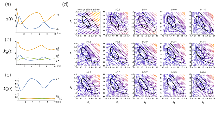
Figure 10: A nonequilibrium trajectory of the Brusselator CRN (Ex. 1) and the associated time-dependent cycle flux $\bm{j}_{st}(t,\bm{x})=\bm{j}_{MA}(\bm{x};\bm{k}^{\pm}_{st}(t))$. (a) A nonequilibrium trajectory $\{\bm{x}_{t}\}$ of the Brusselator CRN obtained with the same parameter values in Fig. 8 (a) . (b,c) The time-dependent kinetic parameter set $\bm{k}^{\pm}_{st}(t)$, which generates the time-dependent cycle flux $\bm{j}_{st}(t,\bm{x})$. (d) The top left panel shows the nonequilibrium trajectory $\{\bm{x}_{t}\}$ (the black curve) and vector field $\bm{v}(\bm{x})=-\mathbb{S}\bm{j}(\bm{x})$ (arrows). The other panels show the time-dependent vector field $\bm{v}_{st}(t,\bm{x})$ induced by $\bm{j}_{st}(t,\bm{x})$: $\bm{v}_{st}(t,\bm{x})=-\mathbb{S}\bm{j}_{st}(t,\bm{x})$. The nonequilibrium trajectory $\{\bm{x}_{t}\}$ is also depicted as for a reference (the black curve). In each panel, the white circle on the trajectory is $\bm{x}_{t}$ at which $\bm{j}_{st}(t,\bm{x})$ is computed.

Example 4 (Simplified Brusselator CRN[8, 107] (continued)).

For the nonequilibrium trajectory of the Brusselator CRN in Fig. 10 (a), we numerically obtained the effective cycle flux $\bm{j}_{st}(t,\bm{x})$ and the corresponding time-dependent kinetic parameter set $\bm{k}_{st}^{\pm}(t)$ (Fig. 10 (b,c)). Figure 10 (d) shows the vector field $\bm{v}_{st}(t,\bm{x})=-\mathbb{S}\bm{j}_{st}(t,\bm{x})$ induced by the effective cycle flux $\bm{j}_{st}(t,\bm{x})$. From Fig. 10, we can see that any point on the trajectory $\{\bm{x}_{t}\}$ originally generated by the nonequilibrium flux $\bm{j}(\bm{x}_{t})$ can be kept steady with the time-dependent cycle flux $\bm{j}_{st}(t,\bm{x})$ realized by the modulation of the kinetic parameter $\bm{k}^{\pm}_{st}(t)$.

In modern nonequilibrium thermodynamics, it has been a great challenge to establish thermodynamic characterizations for nonequilibrium phenomena. To this end, the dissection of dynamics and the corresponding flux and force has been attempted[163, 164, 165, 166, 107]. For a given trajectory $\{\bm{x}_{t}\}$, the effective time-dependent equilibrium flux $\bm{j}_{eq}(t,\bm{x})$ generates exactly the same trajectory, which dissects and mimics the dynamic aspect of the trajectory. On the other hand, the effective time-dependent cycle flux $\bm{j}_{st}(t,\bm{x})$ makes each point on the trajectory steady, which can be recognized as the nonequilibrium aspect of the trajectory. Moreover, these two types of fluxes can be realized by appropriately modulating the kinetic parameter set $\bm{k}^{\pm}$, which makes the dissected fluxes physically meaningful and accessible. More specifically, the modulation of the force part $\bm{K}$ of the kinetic parameter is sufficient for realization (Eq. 156 and Eq. 168) while the activity part $\bm{\kappa}$ is kept constant. In the case of CRN, the former is linked to the free energy difference between reactants and products of each reaction, and the other is associated with the height of the energy barrier between them. This clear separation of different physical parameters in our framework is advantageous to further investigate physical aspects of dynamics on graphs and hypergraphs. Thus, the dually flat structure on the edge space and the HHK decomposition provides a new and promising way to characterize the nonequilibrium flow.

X Summary and Discussion

In this work, we have shown that the doubly dual flat structure of the vertex and edge spaces on graphs and hypergraphs provides the information-geometric basis for the dynamics on graphs and hypergraphs. Two notions of orthogonality, pseudo-Hilbert isosceles orthogonality and information-geometric orthogonality, have been introduced and shown to dissect the equilibrium and nonequilibrium aspects of the dynamics into the induced structures on the tangent and cotangent spaces and the cycle spaces. The doubly dual flat structure naturally connects the topological information of underlying discrete manifolds, i.e., graphs and hypergraphs, with the dynamics on them and thus endows more flexibility and representation power to the information-geometric modeling of dynamics. Furthermore, the generalized equilibrium and nonequilibrium flow, as well as the generalized flow, accommodate a sufficiently wide range of models, which include the reversible Markov jump processes on finite graphs and CRN with LMA kinetics (a class of PDS). These results could substantially extend the applicability of information geometry to dynamical problems.

X.1 Extension of other relations involving information measures

While we demonstrated that the generalized flow and the doubly dual flat structure can extend several results known for FPE and diffusion processes, we still have potentially relevant results and problems that could be explained and extended in our framework. For example, for FPE and diffusion processes, the Fisher information number $\mathbb{I}_{F}$ was extended to the relative Fisher information (also known as Hyvärinen divergence[148, 124]). The relative Fisher information of two trajectories $p^{(1)}_{t}(\bm{r})$ and $p^{(2)}_{t}(\bm{r})$ are known to satisfy information-theoretic relations such as the De Brujin identity[54] and its extensions[62, 56]. In addition, the logarithmic Sobolev inequality also constitutes a relationship between the Fisher information number and the KL divergence (or Shannon information)[63, 64]. It would be an important future problem to associate these results with the doubly dual flat structure.

Moreover, several relations potentially being related to De Giorgi’s formulation (Eq. 52) have been known for mutual information in filtering and control theories. For example, Guo, Shamai, and Verdu found a relation between mutual information and the minimum mean square error (MMSE) in Gaussian channels [167]. Relations similar to these have also been reported by Mayer-Wolf and Zakai[168, 169]. Our framework may offer a unified perspective behind these different types of relation involving information measures.

X.2 Extensions of the doubly dual flat structure

There is also room for extensions of the doubly dual flat structure. While we consider only strictly convex thermodynamic functions and dissipation functions, the strict convexity is not necessarily required, at least for defining the generalized flow and the equilibrium and nonequilibrium flows. Actually, in terms of thermodynamics, the thermodynamic function can be non-strictly convex when a phase transition of the system occurs [120]. The loss of bijectivity via the loss of the strict convexity can happen in complicated and degenerate statistical models[170]. Techniques from algebraic geometry could be employed to address such situations[171].

Moreover, the structure introduced for rLDG and CRN may be extended to irreversible cases, where some edges have only either forward or reverse jumps or reactions. For this purpose, we may take advantage of several results about the CB states obtained in CRN theory [8] where the reversibility is not necessarily assumed and those in stochastic thermodynamics for absolute irreversible processes [172].

While the nonequilibrium flow is general enough to cover at least all reversible CRN with LMA kinetics, the classes of nonlinear dynamics other than CRN are much wider in general. To further extend the range of models that can be covered, GENERIC (General Equation for Non-Equilibrium Reversible-Irreversible Coupling) would be a good candidate [173]. GENERIC is a theoretical framework to integrate dissipative dynamics (gradient flow dynamics) and conservative dynamics (Hamiltonian dynamics). The extension of the generalized flow to GENERIC has already been attempted but is still ongoing [77, 79]. One might also consider Hamiltonian-type dynamics, which differs from the GENERIC structure mentioned above. In the doubly dual flat structure, dual spaces are statically coupled by the Legendre duality. However, we could consider the coupling of two dynamics, each of which is defined on the primal and the dual spaces. Such coupling has been investigated in relation to accelerations of gradient flows[174], optimal control problems[175], and also mean field game problems[176]. It would be quite an interesting problem to formulate this dynamic coupling in relation to our results and also the results of GENERIC. The information geometry could offer new insights and techniques to achieve these missions.

X.3 Homological algebra and differential geometric formulations

From the viewpoint of the standard homological algebra, the doubly dual flat structure that we introduced is an extension of chain and cochain complexes with inner product structure. Because the homological algebra used here is an abstraction of the differential form, the doubly dual flat structure can also be viewed as an extension of the differential form and might be called dually flat form. It would be an interesting mission to characterize this stricture under a more rigorous mathematical formulation and to investigate if the Legendre duality can be consistently introduced for chains and cochains higher than those of the edge space. From the viewpoint of differential geometry, the dual flat structure can be defined independently of the specific coordinate by the Hessian geometry[149]. While we stick to the standard basis of the graph or hypergraph on which the convex thermodynamic function is defined, we can formulate it more generally. It would be an important future work to clarify how the doubly dual flat structure can be formulated from a differential geometric perspective.

X.4 Consistency and Persistence

Finally, we would like to mention the problem of consistency and persistence. In this work, we presume that the flux $\bm{j}(\bm{x})$ is consistent with $\mathbb{H}$ and that the trajectory is persistent. The explicit conditions when these are satisfied are still elusive. Actually, the condition for consistency is intricate, even for the separable cases. For an illustrative example, suppose that the $i$th molecule is involved in the $e$th reaction of a CRN with LMA kinetics. For $x_{i}\to 0$, $j_{e}(\bm{x})\to 0$ holds. However, their Legendre duals diverge as $y_{i}\to-\infty$ and $f_{e}(\bm{x})\to-\infty$. The flux $j_{e}(\bm{x})$ goes to $0$ because $\omega_{e}(\bm{x})\to 0$ holds. This example suggests that we have to consider a certain limit of relevant quantities to appropriately address the consistency condition.

The persistence of the nonequilibrium flow would be a much harder problem. While persistence has been approached for CB CRN with LMA kinetics using techniques from algebraic geometry[115], its connection to information geometry has yet to be clarified. Moreover, from an information-geometric viewpoint, the loss of persistence means a change in the support of probability or positive density, which is effectively accompanied by a change in the topology of the underlying graph or hypergraph. To resolve the problem, we may need a deeper understanding of the interrelationship among dynamics, information-geometric structure, and the underlying topology.

XI Acknowledgement

This research is supported by JST (JPMJCR2011,JPMJCR1927) and JSPS (19H05799). The authors thank Hideyuki Miyahara and Tomonari Sei for their critical comments. We also express our sincere thanks to the anonymous reviewer who carefully read our manuscript and provided valuable comments.

XII Conflict of interest

The authors have no conflict of interest, financial or otherwise.

Appendix A Symbols, Notations, and Abbreviations

$\mathbb{G}$, $\mathbb{G}_{\bm{k}^{\pm}}$	finite graph and edge-weighted finite graph.	Def. 1
$\mathbb{v}$, $\mathbb{e}$	vertex and edges of graph$\mathbb{G}$.	Def. 1
$\mathbb{B}$	incidence matrix	Def. 1
$\mathbb{H}$, $\mathbb{H}_{\bm{k}^{\pm}}$	Reversible CRN hypergraph and edge-weighted hypergraph.	Def. 4
$\mathbb{X}$, $\hat{\mathbb{v}}$, $\mathbb{e}$	vertex, hypervertex, and hyperedges of CRN hypergraph $\mathbb{H}$.	Def. 4
$\mathbb{S}$	Hypergraph incidence matrix.	Def. 4
$\textstyle\mathbb{L}$	Hypervertex matrix	Def. 4
$C_{p}(\mathbb{G})$, $C^{p}(\mathbb{G})$	$p$-chain and $p$-cochain of graph with field $\mathbb{R}$	Sec. III.1
$C_{p}(\mathbb{H})$, $C^{p}(\mathbb{H})$	$p$-chain and $p$-cochain of hypergraph with field $\mathbb{R}$	Def. 9
$\delta_{p}$, $\delta^{p}$	$p$-discrete differentials	Sec. III.1, Def. 9
$\mathrm{grad}_{\mathbb{S}}:=\delta^{0}=\mathbb{S}^{T}$	Discrete gradient	Def. 10
$\mathrm{div}_{\mathbb{S}}=\mathrm{grad}^{*}_{\mathbb{S}}:=\delta_{1}=\mathbb{S}$	Discrete divergence (adjoint of discrete gradient)	Def. 10
$\mathrm{curl}_{\mathbb{V}}:=\delta^{1}=\mathbb{V}^{T}$	Discrete curl	Def. 10
$\mathrm{curl}^{*}_{\mathbb{V}}:=\delta_{2}=\mathbb{V}$	Adjoint of discrete curl	Def. 10

Table 1: List of symbols and notations related to graph, hypergraph, and homological algebra.

$\mathcal{X}$, $\mathcal{Y}$	Primal and dual vertex spaces (density and potential spaces)	Def. 11, Def. 13
$\bm{x}$	The density defined on vertices of graph or hypergraph	Def. 2, Def. 4
$\bm{y}$	The potential field defined on vertices of graph or hypergraph	Def. 13
$\mathcal{J}_{\bm{x}}$, $\mathcal{F}_{\bm{x}}$	Primal and dual edge spaces	Def. 17
$\bm{j}^{+}$, $\bm{j}^{-}$	The forward and reverse oneway fluxes of graph or hypergraph	Def. 2
$\bm{j}$	The total flux on edges of graph or hypergraph	Def. 2
$\bm{f}$	The force on edges of graph or phyergraph	Eq. 36
$j^{\pm}_{\mathrm{MA}}$, $\bm{j}^{\pm}_{\mathrm{eMA}}$	Oneway fluxes of the normal and extended LMA kinetics.	Eq. 12, Eq. 13
$\bm{j}_{\mathrm{FP}}$	Flux of the FPE	Eq. 18
$\bm{f}_{NE}$	Nonequilibrium force	Eq. 60
$\bm{f}_{\mathrm{MA}}(\bm{x};\bm{K})$, $\bm{\omega}_{\mathrm{MA}}(\bm{x};\bm{\kappa})$	Force and frenetic activity of LMA kinetics	Eq. 70
$\mathcal{M}^{\mathrm{ST}}$	Steady state manifold	Eq. 47
$\mathcal{M}^{\mathrm{CB}}$	Complex-balanced manifold	Eq. 47
$\mathcal{M}^{\mathrm{DB}}$	Detailed-balanced manifold	Eq. 47
$\mathcal{L}_{\bm{\theta}}$	Weighted asymmetric graph Laplacian	Def. 3

Table 2: List of symbols and notations related to the dynamics on graph and hypergraph.

$\Phi$, $\Phi^{*}$	Primal and dual thermodynamic functions	Def. 12, Def. 13
$\mathcal{D}^{\mathcal{X}}_{\Phi}[\bm{x}\|\bm{x}^{\prime}]$, $\mathcal{D}^{\mathcal{Y}}_{\Phi^{*}}[\bm{y}^{\prime}\|\bm{y}]$	Bregman divergences on vertex spaces	Def. 14
$\mathcal{T}_{\bm{x}}\mathcal{X}$, $\mathcal{T}^{*}_{\bm{x}}\mathcal{X}$	Tangent and cotangent spaces of $\mathcal{X}$	Def. 15
$\mathcal{T}_{\bm{y}}\mathcal{Y}$, $\mathcal{T}^{*}_{\bm{y}}\mathcal{Y}$	Tangent and cotangent spaces of $\mathcal{Y}$	Def. 15
$G_{\bm{x}}$, $G_{\bm{y}}^{*}$	Hessian matrices on vertex spaces	Def. 15
$\Psi_{\bm{x}}$, $\Psi^{*}_{\bm{x}}$	Primal and dual dissipation functions	Def. 18
$\mathcal{D}_{\bm{x}}^{\mathcal{J},\mathcal{F}}[\bm{j};\bm{f}^{\prime}]$	Bregman divergence on the edge space	Eq. 41
$G_{\bm{x},\bm{j}}$, $G_{\bm{x},\bm{f}}^{*}$	Hessian matrices on the edge space	Eq. 42
$\Psi^{q,*}_{\bm{x}}(\bm{f})$	Quadratic dissipation function	Eq. 43
$\mathcal{P}^{sc}(\bm{x}_{0})$	Stoichiometric subspace	Def. 26
$\mathcal{P}^{eq}(\tilde{\bm{y}})$	Equilibrium subspace	Def. 27
$\mathcal{P}^{vl}(\hat{\bm{j}})$	Iso-velocity subspace	Def. 28
$\mathcal{P}^{fr}(\bm{f}^{\prime})$	Iso-force subspace	Def. 29
$\mathcal{M}^{sc}(\bm{y}_{0})$, $\mathcal{M}^{eq}(\tilde{\bm{x}})$	Stoichiometric and equilibrium manifolds	Def. 30
$\mathcal{M}^{vl}_{\bm{x}}(\hat{\bm{f}})$, $\mathcal{M}^{fr}_{\bm{x}}(\bm{j}^{\prime})$	Iso-velocity and Iso-force manifolds	Def. 31
$\mathcal{C}_{\bm{x}}^{\Psi}(c)$, $\mathcal{C}_{\bm{x}}^{\Psi^{*}}(c)$	Primal central affine manifolds	Def. 32
$\mathcal{M}_{\bm{x}}^{\Psi}(c)$, $\mathcal{M}_{\bm{x}}^{\Psi^{*}}(c)$	Dual central affine manifolds	Def. 120
$\perp_{H}$	Pseudo-Hilbert-isosceles orthogonality	Def. 33
$\tilde{\mathcal{T}}_{\bm{x}}\mathcal{X}$, $\tilde{\mathcal{T}}_{\bm{x}}^{*}\mathcal{X}$	Induced tangent and cotangent spaces of $\mathcal{X}$	Thm. 2
$\tilde{\Psi}_{\bm{x}}(\bm{v})$, $\tilde{\Psi}_{\bm{x}}^{*}(\bm{u})$	Induced dissipation functions on tangent and cotangent spaces	Eq. 132
$\mathcal{Z}_{\bm{x}}$, $\mathfrak{Z}_{\bm{x}}$	Cycle spaces	Def. 34
$\hat{\Psi}_{\bm{x}}(\bm{z})$, $\hat{\Psi}_{\bm{x}}^{*}(\bm{\zeta})$	Induced dissipation functions on cycle spaces	Eq. 162

Table 3: List of symbols and notations related to the information-geometric structure.

CRN	Chemical reaction network
LMA	Law of mass action
(r)MJP	(Reversible) Markov jump process
(r)LDG	(Reversible) linear dynamics on graph
PDS	Polynomial dynamical systems
FPE	Fokker Planck Equation
CB	complex-balanced
DB	detail-balanced
LDB	local detailed balance
EPR	entropy production rate
HHK	Helmholtz-Hodge-Kodaira
MCMC	Markov chain Monte Carlo

Table 4: List of abbreviations.

References

- Amari [2016] S.-i. Amari, Information Geometry and Its Applications (Springer, 2016).
- Ay et al. [2018] N. Ay, P. Gibilisco, and F. Matúš, Information Geometry and Its Applications: On the Occasion of Shun-ichi Amari’s 80th Birthday, IGAIA IV Liblice, Czech Republic, June 2016 (Springer, 2018).
- Risken and Frank [1996] H. Risken and T. Frank, The Fokker-Planck Equation: Methods of Solution and Applications (Springer Science & Business Media, 1996).
- Horsthemke and Lefever [2006] W. Horsthemke and R. Lefever, Noise-Induced Transitions: Theory and Applications in Physics, Chemistry, and Biology (Springer Science & Business Media, 2006).
- Gardiner [2010] C. Gardiner, Stochastic Methods: A Handbook for the Natural and Social Sciences (Springer Berlin Heidelberg, 2010).
- Murray [2007] J. D. Murray, Mathematical Biology: I. An Introduction (Springer Science & Business Media, 2007).
- Beard and Qian [2008] D. A. Beard and H. Qian, Chemical Biophysics: Quantitative Analysis of Cellular Systems, Cambridge Texts in Biomedical Engineering (Cambridge University Press, Cambridge, 2008).
- Feinberg [2019] M. Feinberg, Foundations of Chemical Reaction Network Theory (Springer, 2019).
- Amari [1987a] S. Amari, Differential Geometry in Statistical Inference (Institute of mathematical Statistics, Hayward, Calif, 1987).
- Ravishanker et al. [1990] N. Ravishanker, E. L. Melnick, and C.-L. Tsai, Differential Geometry of Arma Models, J. Time Ser. Anal. 11, 259 (1990).
- Tanaka and Komaki [2011] F. Tanaka and F. Komaki, Asymptotic expansion of the risk difference of the Bayesian spectral density in the autoregressive moving average model, Sankhya A 73, 162 (2011).
- Amari [1987b] S.-i. Amari, Differential geometry of a parametric family of invertible linear systems–Riemannian metric, dual affine connections, and divergence, Math. Systems Theory 20, 53 (1987b).
- Amari [2001] S.-I. Amari, Information geometry on hierarchy of probability distributions, IEEE Trans. Inf. Theory 47, 1701 (2001).
- Nakagawa and Kanaya [1993] K. Nakagawa and F. Kanaya, On the converse theorem in statistical hypothesis testing for Markov chains, IEEE Trans. Inf. Theory 39, 629 (1993).
- Takeuchi and Barron [1998] J. Takeuchi and A. Barron, Asymptotically minimax regret by Bayes mixtures, in Proc. 1998 IEEE Int. Symp. Inf. Theory Cat No98CH36252 (1998) pp. 318–.
- Nagaoka [2017] H. Nagaoka, The exponential family of Markov chains and its information geometry (2017), arxiv:1701.06119 [cs, math] .
- Takeuchi and Kawabata [2007] J. Takeuchi and T. Kawabata, Exponential Curvature of Markov Models, in 2007 IEEE Int. Symp. Inf. Theory (2007) pp. 2891–2895.
- Hayashi and Watanabe [2016] M. Hayashi and S. Watanabe, Information geometry approach to parameter estimation in Markov chains, Ann. Stat. 44, 1495 (2016).
- Wolfer and Watanabe [2021] G. Wolfer and S. Watanabe, Information Geometry of Reversible Markov Chains, Info. Geo. 4, 393 (2021).
- Pistone and Rogantin [2013] G. Pistone and M. P. Rogantin, The algebra of reversible Markov chains, Ann Inst Stat Math 65, 269 (2013).
- Obata et al. [1992] T. Obata, H. Hara, and K. Endo, Differential geometry of nonequilibrium processes, Phys. Rev. A 45, 6997 (1992).
- Ohara [2009] A. Ohara, Geometric study for the Legendre duality of generalized entropies and its application to the porous medium equation, Eur. Phys. J. B 70, 15 (2009).
- Ohara and Zhang [2021] A. Ohara and X. Zhang, Properties of Nonlinear Diffusion Equations on Networks and Their Geometric Aspects, in Geom. Sci. Inf., Lecture Notes in Computer Science, edited by F. Nielsen and F. Barbaresco (Springer International Publishing, Cham, 2021) pp. 736–743.
- Nakamura [1993] Y. Nakamura, Completely integrable gradient systems on the manifolds of Gaussian and multinomial distributions, Japan J. Indust. Appl. Math. 10, 179 (1993).
- Fujiwara and Amari [1995] A. Fujiwara and S.-i. Amari, Gradient systems in view of information geometry, Physica D: Nonlinear Phenomena 80, 317 (1995).
- Felice and Ay [2018] D. Felice and N. Ay, Dynamical Systems induced by Canonical Divergence in dually flat manifolds (2018), arxiv:1812.04461 [math-ph] .
- Goto and Wada [2018] S.-i. Goto and T. Wada, Hessian–information geometric formulation of Hamiltonian systems and generalized Toda’s dual transform, J. Phys. A: Math. Theor. 51, 324001 (2018).
- Chirco et al. [2022] G. Chirco, L. Malagò, and G. Pistone, Lagrangian and Hamiltonian Mechanics for Probabilities on the Statistical Manifold, Int. J. Geom. Methods Mod. Phys. , 2250214 (2022), arxiv:2009.09431 [hep-th, stat] .
- Ihara [1993] S. Ihara, Information Theory for Continuous Systems (World Scientific, 1993).
- Brigo et al. [1999] D. Brigo, B. Hanzon, and F. L. Gland, Approximate nonlinear filtering by projection on exponential manifolds of densities, Bernoulli 5, 495 (1999).
- Newton [2018] N. J. Newton, Nonlinear Filtering and Information Geometry: A Hilbert Manifold Approach, in Inf. Geom. Its Appl., Springer Proceedings in Mathematics & Statistics, edited by N. Ay, P. Gibilisco, and F. Matúš (Springer International Publishing, Cham, 2018) pp. 189–208.
- Fleming and Mitter [1982] W. H. Fleming and S. K. Mitter, Optimal Control and Nonlinear Filtering for Nondegenerate Diffusion Processes, Stochastics 8, 63 (1982).
- Todorov [2009] E. Todorov, Efficient computation of optimal actions, Proc. Natl. Acad. Sci. 106, 11478 (2009).
- Theodorou and Todorov [2012] E. A. Theodorou and E. Todorov, Relative entropy and free energy dualities: Connections to Path Integral and KL control, in 2012 IEEE 51st IEEE Conf. Decis. Control CDC (2012) pp. 1466–1473.
- Jaynes [1957] E. T. Jaynes, Information Theory and Statistical Mechanics, Phys. Rev. 106, 620 (1957).
- Frieden [2004] B. R. Frieden, Science from Fisher Information: A Unification (Cambridge University Press, Cambridge, 2004).
- Sagawa [2012] T. Sagawa, Thermodynamics of Information Processing in Small Systems (Springer Science & Business Media, 2012).
- Kullback and Leibler [1951] S. Kullback and R. A. Leibler, On Information and Sufficiency, Ann. Math. Stat. 22, 79 (1951).
- Lebowitz and Bergmann [1957] J. L. Lebowitz and P. G. Bergmann, Irreversible gibbsian ensembles, Annals of Physics 1, 1 (1957).
- Shear [1967] D. Shear, An analog of the Boltzmann H-theorem (a Liapunov function) for systems of coupled chemical reactions, Journal of Theoretical Biology 16, 212 (1967).
- Horn and Jackson [1972] F. Horn and R. Jackson, General mass action kinetics, Arch. Rational Mech. Anal. 47, 81 (1972).
- Goh [1977] B. S. Goh, Global Stability in Many-Species Systems, Am. Nat. 111, 135 (1977).
- Figueiredo et al. [2000] A. Figueiredo, I. M. Gléria, and T. M. Rocha Filho, Boundedness of solutions and Lyapunov functions in quasi-polynomial systems, Physics Letters A 268, 335 (2000).
- Gibbs [2010] J. W. Gibbs, Elementary Principles in Statistical Mechanics: Developed with Especial Reference to the Rational Foundation of Thermodynamics, Cambridge Library Collection - Mathematics (Cambridge University Press, Cambridge, 2010).
- Waage and Gulberg [1986] P. Waage and C. M. Gulberg, Studies concerning affinity, J. Chem. Educ. 63, 1044 (1986).
- Ge and Qian [2016] H. Ge and H. Qian, Nonequilibrium thermodynamic formalism of nonlinear chemical reaction systems with Waage–Guldberg’s law of mass action, Chemical Physics 472, 241 (2016).
- Rao and Esposito [2016] R. Rao and M. Esposito, Nonequilibrium Thermodynamics of Chemical Reaction Networks: Wisdom from Stochastic Thermodynamics, Phys. Rev. X 6, 041064 (2016).
- Sughiyama et al. [2021a] Y. Sughiyama, D. Loutchko, A. Kamimura, and T. J. Kobayashi, A Hessian Geometric Structure of Chemical Thermodynamic Systems with Stoichiometric Constraints, ArXiv211212403 Cond-Mat Physicsphysics (2021a), arxiv:2112.12403 [cond-mat, physics:physics] .
- Seifert [2012] U. Seifert, Stochastic thermodynamics, fluctuation theorems and molecular machines, Rep. Prog. Phys. 75, 126001 (2012).
- Ito [2018] S. Ito, Stochastic Thermodynamic Interpretation of Information Geometry, Phys. Rev. Lett. 121, 030605 (2018).
- Kolchinsky and Wolpert [2021] A. Kolchinsky and D. H. Wolpert, Work, Entropy Production, and Thermodynamics of Information under Protocol Constraints, Phys. Rev. X 11, 041024 (2021).
- Yoshimura and Ito [2021] K. Yoshimura and S. Ito, Information geometric inequalities of chemical thermodynamics, Phys. Rev. Research 3, 013175 (2021).
- Ohga and Ito [2021] N. Ohga and S. Ito, Information-geometric Legendre duality in stochastic thermodynamics, ArXiv211211008 Cond-Mat (2021), arxiv:2112.11008 [cond-mat] .
- Stam [1959] A. J. Stam, Some inequalities satisfied by the quantities of information of Fisher and Shannon, Information and Control 2, 101 (1959).
- Plastino et al. [1998] A. R. Plastino, M. Casas, and A. Plastino, Fisher’s information, Kullback’s measure, and H-theorems, Physics Letters A 246, 498 (1998).
- Wibisono et al. [2017] A. Wibisono, V. Jog, and P.-L. Loh, Information and estimation in Fokker-Planck channels, in 2017 IEEE Int. Symp. Inf. Theory ISIT (2017) pp. 2673–2677.
- Fisher and Russell [1922] R. A. Fisher and E. J. Russell, On the mathematical foundations of theoretical statistics, Philos. Trans. R. Soc. Lond. Ser. Contain. Pap. Math. Phys. Character 222, 309 (1922).
- Rao [1958] B. R. Rao, On an analogue of Cramér-Rao’s inequality, Scand. Actuar. J. 1958, 57 (1958).
- Papaioannou and Ferentinos [2005] T. Papaioannou and K. Ferentinos, On Two Forms of Fisher’s Measure of Information, Commun. Stat. - Theory Methods 34, 1461 (2005).
- Kharazmi and Asadi [2018] O. Kharazmi and M. Asadi, On the time-dependent Fisher information of a density function, Braz. J. Probab. Stat. 32, 795 (2018).
- Johnson [2004] O. Johnson, Information Theory and the Central Limit Theorem (World Scientific, 2004).
- Yamano [2013a] T. Yamano, De Bruijn-type identity for systems with flux, Eur. Phys. J. B 86, 363 (2013a).
- Gross [1975a] L. Gross, Logarithmic Sobolev Inequalities, Am. J. Math. 97, 1061 (1975a), 2373688 .
- Gross [1975b] L. Gross, Hypercontractivity and logarithmic Sobolev inequalities for the Clifford-Dirichlet form, Duke Math. J. 42, 383 (1975b).
- Otto [2001] F. Otto, The Geometry of Dissipative Evolution Equations: The Porous Medium Equation, Commun. Partial Differ. Equ. 26, 101 (2001).
- Villani [2003] C. Villani, Topics in Optimal Transportation (American Mathematical Soc., 2003).
- Amari [1998] S.-i. Amari, Natural Gradient Works Efficiently in Learning, Neural Computation 10, 251 (1998).
- Beck and Teboulle [2003] A. Beck and M. Teboulle, Mirror descent and nonlinear projected subgradient methods for convex optimization, Operations Research Letters 31, 167 (2003).
- Raskutti and Mukherjee [2015] G. Raskutti and S. Mukherjee, The Information Geometry of Mirror Descent, IEEE Trans. Inf. Theory 61, 1451 (2015).
- Ollivier et al. [2017] Y. Ollivier, L. Arnold, A. Auger, and N. Hansen, Information-Geometric Optimization Algorithms: A Unifying Picture via Invariance Principles, J. Mach. Learn. Res. 18, 1 (2017).
- Hino et al. [2022] H. Hino, S. Akaho, and N. Murata, Geometry of EM and related iterative algorithms, Info. Geo. 10.1007/s41884-022-00080-y (2022).
- Pistone [2021] G. Pistone, Information Geometry of Smooth Densities on the Gaussian Space: Poincaré Inequalities, in Progress in Information Geometry: Theory and Applications, Signals and Communication Technology, edited by F. Nielsen (Springer International Publishing, Cham, 2021) pp. 1–17.
- Grady and Polimeni [2010] L. J. Grady and J. R. Polimeni, Discrete Calculus: Applied Analysis on Graphs for Computational Science (Springer Science & Business Media, 2010).
- Musielak [1983] J. Musielak, Orlicz Spaces and Modular Spaces (Springer, 1983).
- Mielke et al. [2014] A. Mielke, M. A. Peletier, and D. R. M. Renger, On the Relation between Gradient Flows and the Large-Deviation Principle, with Applications to Markov Chains and Diffusion, Potential Anal 41, 1293 (2014).
- Mielke et al. [2017] A. Mielke, R. I. A. Patterson, M. A. Peletier, and D. R. Michiel Renger, Non-equilibrium Thermodynamical Principles for Chemical Reactions with Mass-Action Kinetics, SIAM J. Appl. Math. 77, 1562 (2017).
- Renger [2018] D. R. M. Renger, Gradient and GENERIC Systems in the Space of Fluxes, Applied to Reacting Particle Systems, Entropy 20, 596 (2018).
- Kaiser et al. [2018] M. Kaiser, R. L. Jack, and J. Zimmer, Canonical Structure and Orthogonality of Forces and Currents in Irreversible Markov Chains, J Stat Phys 170, 1019 (2018).
- Patterson et al. [2021] R. I. A. Patterson, D. R. M. Renger, and U. Sharma, Variational structures beyond gradient flows: A macroscopic fluctuation-theory perspective, ArXiv210314384 Math-Ph (2021), arxiv:2103.14384 [math-ph] .
- Peletier et al. [2022] M. A. Peletier, R. Rossi, G. Savaré, and O. Tse, Jump processes as generalized gradient flows, Calc. Var. 61, 33 (2022).
- Renger and Zimmer [2021] D. R. M. Renger and J. Zimmer, Orthogonality of fluxes in general nonlinear reaction networks, Discrete Contin. Dyn. Syst. - S 14, 205 (2021).
- Peletier and Schlichting [2023] M. A. Peletier and A. Schlichting, Cosh gradient systems and tilting, Nonlinear Analysis Variational Models for Discrete Systems, 231, 113094 (2023).
- Kobayashi et al. [2022a] T. J. Kobayashi, D. Loutchko, A. Kamimura, and Y. Sughiyama, Hessian geometry of nonequilibrium chemical reaction networks and entropy production decompositions, Phys. Rev. Research 4, 033208 (2022a).
- Kobayashi et al. [2022b] T. J. Kobayashi, D. Loutchko, A. Kamimura, and Y. Sughiyama, Kinetic derivation of the Hessian geometric structure in chemical reaction networks, Phys. Rev. Research 4, 033066 (2022b).
- Sughiyama et al. [2022a] Y. Sughiyama, D. Loutchko, A. Kamimura, and T. J. Kobayashi, Hessian geometric structure of chemical thermodynamic systems with stoichiometric constraints, Phys. Rev. Research 4, 033065 (2022a).
- Sughiyama et al. [2022b] Y. Sughiyama, A. Kamimura, D. Loutchko, and T. J. Kobayashi, Chemical thermodynamics for growing systems, Phys. Rev. Research 4, 033191 (2022b).
- Godsil and Royle [2013] C. Godsil and G. F. Royle, Algebraic Graph Theory (Springer Science & Business Media, 2013).
- Bretto [2013] A. Bretto, Hypergraph Theory: An Introduction (Springer Science & Business Media, 2013).
- Meyn and Tweedie [2009] S. Meyn and R. L. Tweedie, Markov Chains and Stochastic Stability (Cambridge University Press, 2009).
- Schnakenberg [1976] J. Schnakenberg, Network theory of microscopic and macroscopic behavior of master equation systems, Rev. Mod. Phys. 48, 571 (1976).
- Craciun [2019] G. Craciun, Polynomial Dynamical Systems, Reaction Networks, and Toric Differential Inclusions (2019), arxiv:1901.02544 [math] .
- Biggs [1997] N. Biggs, Algebraic Potential Theory on Graphs, Bull. Lond. Math. Soc. 29, 641 (1997).
- Chung and Graham [1997] F. R. K. Chung and F. C. Graham, Spectral Graph Theory (American Mathematical Soc., 1997).
- Dörfler et al. [2018] F. Dörfler, J. W. Simpson-Porco, and F. Bullo, Electrical Networks and Algebraic Graph Theory: Models, Properties, and Applications, Proc. IEEE 106, 977 (2018).
- Saber and Murray [2003] R. Saber and R. Murray, Consensus protocols for networks of dynamic agents, in Proc. 2003 Am. Control Conf. 2003, Vol. 2 (2003) pp. 951–956.
- Veerman and Lyons [2020] J. J. P. Veerman and R. Lyons, A Primer on Laplacian Dynamics in Directed Graphs (2020), arxiv:2002.02605 [math] .
- Qian and Ge [2021] H. Qian and H. Ge, Stochastic Chemical Reaction Systems in Biology (Springer Nature, 2021).
- Keener and Sneyd [2008] J. Keener and J. Sneyd, Mathematical Physiology: I: Cellular Physiology (Springer Science & Business Media, 2008).
- Sottile [2008] F. Sottile, Toric ideals, real toric varieties, and the algebraic moment map, arXiv:math/0212044 (2008), arxiv:math/0212044 .
- Cox et al. [2011] D. A. Cox, J. B. Little, and H. K. Schenck, Toric Varieties (American Mathematical Soc., 2011).
- Craciun et al. [2009] G. Craciun, A. Dickenstein, A. Shiu, and B. Sturmfels, Toric dynamical systems, Journal of Symbolic Computation In Memoriam Karin Gatermann, 44, 1551 (2009).
- Kobayashi et al. [2021] T. J. Kobayashi, D. Loutchko, A. Kamimura, and Y. Sughiyama, Kinetic Derivation of the Hessian Geometric Structure in Chemical Reaction Systems, ArXiv211214910 Phys. (2021), arxiv:2112.14910 [physics] .
- Pachter and Sturmfels [2005] L. Pachter and B. Sturmfels, eds., Algebraic Statistics for Computational Biology (Cambridge University Press, Cambridge, 2005).
- Rapallo [2007] F. Rapallo, Toric statistical models: Parametric and binomial representations, AISM 59, 727 (2007).
- Müller and Regensburger [2012] S. Müller and G. Regensburger, Generalized Mass Action Systems: Complex Balancing Equilibria and Sign Vectors of the Stoichiometric and Kinetic-Order Subspaces, SIAM J. Appl. Math. 72, 1926 (2012).
- Noor et al. [2013] E. Noor, A. Flamholz, W. Liebermeister, A. Bar-Even, and R. Milo, A note on the kinetics of enzyme action: A decomposition that highlights thermodynamic effects, FEBS Letters A Century of Michaelis - Menten Kinetics, 587, 2772 (2013).
- Yoshimura et al. [2023] K. Yoshimura, A. Kolchinsky, A. Dechant, and S. Ito, Housekeeping and excess entropy production for general nonlinear dynamics, Phys. Rev. Res. 5, 013017 (2023).
- Lim [2020] L.-H. Lim, Hodge Laplacians on Graphs, SIAM Rev. 62, 685 (2020).
- Sunada [2012] T. Sunada, Topological Crystallography: With a View Towards Discrete Geometric Analysis (Springer Science & Business Media, 2012).
- Desbrun et al. [2005] M. Desbrun, A. N. Hirani, M. Leok, and J. E. Marsden, Discrete Exterior Calculus (2005), arxiv:math/0508341 .
- Hirani [2003] A. N. Hirani, Discrete Exterior Calculus, Ph.D. thesis, California Institute of Technology (2003).
- Knauer [2011] U. Knauer, Algebraic Graph Theory: Morphisms, Monoids and Matrices (Walter de Gruyter, 2011).
- Chen [2012] W.-K. Chen, Applied Graph Theory (Elsevier, 2012).
- Craciun et al. [2013] G. Craciun, F. Nazarov, and C. Pantea, Persistence and Permanence of Mass-Action and Power-Law Dynamical Systems, SIAM J. Appl. Math. 73, 305 (2013).
- Craciun [2016] G. Craciun, Toric Differential Inclusions and a Proof of the Global Attractor Conjecture (2016), arxiv:1501.02860 [math] .
- Bregman [1967] L. M. Bregman, The relaxation method of finding the common point of convex sets and its application to the solution of problems in convex programming, USSR Computational Mathematics and Mathematical Physics 7, 200 (1967).
- Rockafellar [1997] R. T. Rockafellar, Convex Analysis (Princeton University Press, 1997).
- Mitroi and Niculescu [2011] F.-C. Mitroi and C. P. Niculescu, An Extension of Young’s Inequality, Abstr. Appl. Anal. 2011, e162049 (2011).
- Nielsen [2021] F. Nielsen, On Geodesic Triangles with Right Angles in a Dually Flat Space, in Progress in Information Geometry: Theory and Applications, Signals and Communication Technology, edited by F. Nielsen (Springer International Publishing, Cham, 2021) pp. 153–190.
- Callen and Callen [1985] H. B. Callen and H. B. Callen, Thermodynamics and an Introduction to Thermostatistics (Wiley, 1985).
- Sughiyama et al. [2021b] Y. Sughiyama, D. Loutchko, A. Kamimura, and T. J. Kobayashi, A Hessian Geometric Structure of Chemical Thermodynamic Systems with Stoichiometric Constraints, ArXiv211212403 Cond-Mat Physicsphysics (2021b), arxiv:2112.12403 [cond-mat, physics:physics] .
- Hiriart-Urruty and Lemarechal [1996] J.-B. Hiriart-Urruty and C. Lemarechal, Convex Analysis and Minimization Algorithms II: Advanced Theory and Bundle Methods (Springer Science & Business Media, 1996).
- Krasnosel’skij and Rutickij [1962] M. A. Krasnosel’skij and J. B. Rutickij, Convex Functions and Orlicz Spaces (Hindustan Publ., 1962).
- Lods and Pistone [2015] B. Lods and G. Pistone, Information Geometry Formalism for the Spatially Homogeneous Boltzmann Equation, Entropy 17, 4323 (2015).
- Pistone [2018] G. Pistone, Information Geometry of the Gaussian Space, in Inf. Geom. Its Appl., Springer Proceedings in Mathematics & Statistics, edited by N. Ay, P. Gibilisco, and F. Matúš (Springer International Publishing, Cham, 2018) pp. 119–155.
- Ambrosio et al. [2006] L. Ambrosio, N. Gigli, and G. Savare, Gradient Flows: In Metric Spaces and in the Space of Probability Measures (Springer Science & Business Media, 2006).
- Liero et al. [2016] M. Liero, A. Mielke, and G. Savaré, Optimal Transport in Competition with Reaction: The Hellinger–Kantorovich Distance and Geodesic Curves, SIAM J. Math. Anal. 48, 2869 (2016).
- Onsager [1931a] L. Onsager, Reciprocal Relations in Irreversible Processes. I., Phys. Rev. 37, 405 (1931a).
- Onsager [1931b] L. Onsager, Reciprocal Relations in Irreversible Processes. II., Phys. Rev. 38, 2265 (1931b).
- Machlup and Onsager [1953] S. Machlup and L. Onsager, Fluctuations and Irreversible Process. II. Systems with Kinetic Energy, Phys. Rev. 91, 1512 (1953).
- Lisini [2009] S. Lisini, Nonlinear diffusion equations with variable coefficients as gradient flows in Wasserstein spaces, ESAIM: COCV 15, 712 (2009).
- Peletier [2014] M. A. Peletier, Variational Modelling: Energies, gradient flows, and large deviations (2014), arxiv:1402.1990 [math-ph] .
- Truesdell et al. [2004] C. A. Truesdell, C. Truesdell, W. Noll, S. Antman, and W. Noll, The Non-Linear Field Theories of Mechanics (Springer Science & Business Media, 2004).
- Bergmann and Lebowitz [1955] P. G. Bergmann and J. L. Lebowitz, New Approach to Nonequilibrium Processes, Phys. Rev. 99, 578 (1955).
- Maes [2021] C. Maes, Local detailed balance, SciPost Phys. Lect. Notes , 032 (2021).
- Maes [2017] C. Maes, Non-Dissipative Effects in Nonequilibrium Systems (Springer, 2017).
- Patterson and Renger [2019] R. Patterson and M. Renger, Large deviations of reaction fluxes, Math Phys Anal Geom 22, 21 (2019), arxiv:1802.02512 [math] .
- Wegscheider [1902] R. Wegscheider, Über simultane Gleichgewichte und die Beziehungen zwischen Thermodynamik und Reaktionskinetik homogener Systeme, Z. Für Phys. Chem. 39U, 257 (1902).
- Pistone and Sempi [1995] G. Pistone and C. Sempi, An Infinite-Dimensional Geometric Structure on the Space of all the Probability Measures Equivalent to a Given One, Ann. Stat. 23, 1543 (1995).
- Pistone [2013] G. Pistone, Examples of the Application of Nonparametric Information Geometry to Statistical Physics, Entropy 15, 4042 (2013).
- Shiraishi [2021] N. Shiraishi, Optimal Thermodynamic Uncertainty Relation in Markov Jump Processes, J Stat Phys 185, 19 (2021).
- Chow et al. [2012] S.-N. Chow, W. Huang, Y. Li, and H. Zhou, Fokker–Planck Equations for a Free Energy Functional or Markov Process on a Graph, Arch Rational Mech Anal 203, 969 (2012).
- Maas [2011] J. Maas, Gradient flows of the entropy for finite Markov chains, Journal of Functional Analysis 261, 2250 (2011).
- Mielke [2013] A. Mielke, Geodesic convexity of the relative entropy in reversible Markov chains, Calc. Var. 48, 1 (2013).
- Liero and Mielke [2013] M. Liero and A. Mielke, Gradient structures and geodesic convexity for reaction–diffusion systems, Philos. Trans. R. Soc. Math. Phys. Eng. Sci. 371, 20120346 (2013).
- Van Vu and Saito [2023] T. Van Vu and K. Saito, Thermodynamic Unification of Optimal Transport: Thermodynamic Uncertainty Relation, Minimum Dissipation, and Thermodynamic Speed Limits, Phys. Rev. X 13, 011013 (2023).
- Yamano [2013b] T. Yamano, Phase space gradient of dissipated work and information: A role of relative Fisher information, J. Math. Phys. 54, 113301 (2013b).
- Hyvärinen [2005] A. Hyvärinen, Estimation of Non-Normalized Statistical Models by Score Matching, J. Mach. Learn. Res. 6, 695 (2005).
- Shima [2007] H. Shima, The Geometry of Hessian Structures (World Scientific, 2007).
- Wolsey and Nemhauser [1999] L. A. Wolsey and G. L. Nemhauser, Integer and Combinatorial Optimization (John Wiley & Sons, 1999).
- Davis [1959] H. F. Davis, On Isosceles Orthogonality, Math. Mag. 32, 129 (1959), 3029494 .
- Amari [1996] S.-I. Amari, Neural learning in structured parameter spaces: Natural Riemannian gradient, in Proc. 9th Int. Conf. Neural Inf. Process. Syst., NIPS’96 (MIT Press, Cambridge, MA, USA, 1996) pp. 127–133.
- Gunasekar et al. [2021] S. Gunasekar, B. Woodworth, and N. Srebro, Mirrorless Mirror Descent: A Natural Derivation of Mirror Descent, in Proc. 24th Int. Conf. Artif. Intell. Stat. (PMLR, 2021) pp. 2305–2313.
- Li and Montúfar [2018] W. Li and G. Montúfar, Natural gradient via optimal transport, Info. Geo. 1, 181 (2018).
- Amari et al. [2018] S.-i. Amari, R. Karakida, and M. Oizumi, Information geometry connecting Wasserstein distance and Kullback–Leibler divergence via the entropy-relaxed transportation problem, Info. Geo. 1, 13 (2018).
- Bain and Crisan [2008] A. Bain and D. Crisan, Fundamentals of Stochastic Filtering (Springer Science & Business Media, 2008).
- Brigo et al. [1998] D. Brigo, B. Hanzon, and F. LeGland, A differential geometric approach to nonlinear filtering: The projection filter, IEEE Trans. Autom. Control 43, 247 (1998).
- Li et al. [2017] Y. Li, Y. Cheng, X. Li, H. Wang, X. Hua, and Y. Qin, Information geometric approach for nonlinear filtering, in 2017 36th Chin. Control Conf. CCC (2017) pp. 1211–1216.
- Hill [2005] T. L. Hill, Free Energy Transduction and Biochemical Cycle Kinetics (Courier Corporation, 2005).
- Altaner et al. [2012] B. Altaner, S. Grosskinsky, S. Herminghaus, L. Katthän, M. Timme, and J. Vollmer, Network representations of nonequilibrium steady states: Cycle decompositions, symmetries, and dominant paths, Phys. Rev. E 85, 041133 (2012).
- Polettini and Esposito [2014] M. Polettini and M. Esposito, Irreversible thermodynamics of open chemical networks. I. Emergent cycles and broken conservation laws, J. Chem. Phys. 141, 024117 (2014).
- Strang [2020] A. Strang, Applications of the Helmholtz-Hodge Decomposition to Networks and Random Processes, Ph.D. thesis, Ann Arbor, United States (2020).
- Oono and Paniconi [1998] Y. Oono and M. Paniconi, Steady State Thermodynamics, Progress of Theoretical Physics Supplement 130, 29 (1998).
- Komatsu et al. [2008] T. S. Komatsu, N. Nakagawa, S.-i. Sasa, and H. Tasaki, Steady-State Thermodynamics for Heat Conduction: Microscopic Derivation, Phys. Rev. Lett. 100, 230602 (2008).
- Maes and Netočný [2014] C. Maes and K. Netočný, A Nonequilibrium Extension of the Clausius Heat Theorem, J Stat Phys 154, 188 (2014).
- Dechant et al. [2022] A. Dechant, S.-i. Sasa, and S. Ito, Geometric decomposition of entropy production in out-of-equilibrium systems, ArXiv210912817 Cond-Mat (2022), arxiv:2109.12817 [cond-mat] .
- Guo et al. [2005] D. Guo, S. Shamai, and S. Verdu, Mutual information and minimum mean-square error in Gaussian channels, IEEE Trans. Inf. Theory 51, 1261 (2005).
- Mayer-Wolf and Zakai [1984] E. Mayer-Wolf and M. Zakai, On a formula relating the Shannon information to the fisher information for the filtering problem, in Filter. Control Random Process., Lecture Notes in Control and Information Sciences, edited by H. Korezlioglu, G. Mazziotto, and J. Szpirglas (Springer, Berlin, Heidelberg, 1984) pp. 164–171.
- Mayer-Wolf and Zakai [2007] E. Mayer-Wolf and M. Zakai, Some relations between mutual information and estimation error in Wiener space, Ann. Appl. Probab. 17, 1102 (2007).
- Amari et al. [2006] S.-i. Amari, H. Park, and T. Ozeki, Singularities Affect Dynamics of Learning in Neuromanifolds, Neural Computation 18, 1007 (2006).
- Watanabe [2009] S. Watanabe, Algebraic Geometry and Statistical Learning Theory (Cambridge University Press, 2009).
- Murashita et al. [2014] Y. Murashita, K. Funo, and M. Ueda, Nonequilibrium equalities in absolutely irreversible processes, Phys. Rev. E 90, 042110 (2014).
- Öttinger [2005] H. C. Öttinger, Beyond Equilibrium Thermodynamics (John Wiley & Sons, 2005).
- Wang and Li [2021] Y. Wang and W. Li, Accelerated Information Gradient Flow, J Sci Comput 90, 11 (2021).
- Li et al. [2023] W. Li, S. Liu, and S. Osher, Controlling conservation laws I: Entropy–entropy flux, J. Comput. Phys. 480, 10.1016/j.jcp.2023.112019 (2023).
- Gao et al. [2022] Y. Gao, W. Li, and J.-G. Liu, Master equations for finite state mean field games with nonlinear activations (2022), arxiv:2212.05675 [math] .