Dual gradient method for ill-posed problems using multiple repeated measurement data
Abstract.
We consider determining -minimizing solutions of linear ill-posed problems , where is a bounded linear operator from a Banach space to a Hilbert space and is a proper strongly convex penalty function. Assuming that multiple repeated independent identically distributed unbiased data of are available, we consider a dual gradient method to reconstruct the -minimizing solution using the average of these data. By terminating the method by either an a priori stopping rule or a statistical variant of the discrepancy principle, we provide the convergence analysis and derive convergence rates when the sought solution satisfies certain variational source conditions. Various numerical results are reported to test the performance of the method.
1. Introduction
Inverse problems arise from many practical applications in science and engineering when one aims at determining unobservable causes from observed effects. Due to their significance in wide range of applications, inverse problems have received tremendous attention in the literature.
In this paper we will consider linear inverse problems of the form
| (1.1) |
where is a bounded linear operator from a Banach space to a Hilbert space . Throughout the paper we will assume that , the range of , which guarantees (1.1) has a solution. However, (1.1) may have many solutions. In order to find a solution with desired feature, by incorporating a priori available information we take a proper, lower semi-continuous, convex function and search for a solution of (1.1) satisfying
| (1.2) |
which is called a -minimizing solution of (1.1).
In practical applications, the exact data is generally unknown. Very often, we only have corrupted measurement data at hand. Due to the inherent ill-posedness property of inverse problems, the -minimizing solution of (1.1) may not depend continuously on the data. How to use the noisy data to reconstruct the sought solution therefore becomes a central topic in computational inverse problems.
To conquer ill-posedness, many iterative regularization methods have been developed to solve inverse problems using noisy data; see [4, 8, 10, 23, 24, 32] for instance. The performance of these methods depends crucially on a proper termination of the iterations. In case an accurate upper bound of noise level is available, various a posteriori rules, including the prominent discrepancy principle, have been proposed to choose the stopping index of iteration. In case the information on noise level is difficult to infer, one has to resort to the so-called heuristic rules ([12, 20, 21, 25, 26]) which use only the noisy data to select a termination index. Although Bakushiski’s veto ([1]) states that heuristic rules can not lead to convergence in the sense of worst case scenario for any regularisation method, such rules often work as well as, or even better than, the rules using information on noise level. The drawback of a heuristic rule is that it chooses a stopping index of iteration based on minimizing a function over for which the existence of a minimizer can not be guaranteed unless the noisy data satisfies certain restrictive conditions.
In this paper we assume that the data can be measured multiple times repeatedly and the sought solution does not change during the measurement. This is a common practice in applications where the experiments are set up to allow acquiring multiple observation data by repeating the experiments. Therefore, instead of the unknown exact data , we are given multiple unbiased measurements of which are independent identically distributed -valued random variables. Based on these multiple measurements, for each we use
| (1.3) |
as an estimator of . We then use to construct regularized solutions and consider their behavior as .
Using the average of multiple measurements to decrease the data error is a standard noise reduction technique in engineering which is called the signal averaging method ([14, 29, 35]). Assume are -valued random variables defined on a probability space with denoting the expectation. If are unbiased, independent, identically distributed estimators of with a finite variance , we have
which demonstrates that using as an estimator of can reduce the variance by a factor of . Therefore, it is reasonable to expect more accurate approximate solution can be constructed using the averaged data than using an individual data .
In [13] a general class of linear spectral regularization methods have been considered for solving linear ill-posed problems in Hilbert spaces using the average of multiple measurement data. Without using any knowledge of the noise distribution, the convergence and rates of convergence of the regularized solutions, as the number of measurements increases, have been provided under either an a priori parameter choice rule or the discrepancy principle. The results obtained in [13] can be applied mainly for (1.2) with being a Hilbert space and . In many applications, however, the sought solution may sit in a Banach space instead of a Hilbert space, and the sought solution may have a priori known special features, such as nonnegativity, sparsity and piecewise constancy. Therefore, it is necessary to develop regularization methods using multiple repeated measurement data for finding a -minimizing solution of (1.1) in a general Banach space with a general convex penalty function .
In this paper we will consider a dual gradient method for solving (1.2) using multiple repeated measurement data. When the exact data is available, this method can be derived by applying the gradient method to the dual problem of (1.2) and it takes the form (see [22])
| (1.4) | ||||
with the initial guess , where denotes the adjoint of and is a step-size. This method actually belongs to the class of Uzawa methods, see [2, 33, 34]. This method also has connection to the mirror descent method, see [4, 22, 24, 30]. In case the exact data is unavailable and we are given multiple repeated random measurement data , we may define by (1.3) for each and replace in (1.4) by to obtain
| (1.5) | ||||
with the initial guess and a step size . This is the dual gradient method that we will consider for solving (1.2) using the average of multiple random measurement data. Since are random variables, we need to consider the convergence of (1.5) based on a stochastic analysis.
When is a Hilbert space and , the method (1.5) becomes the Landweber iteration in Hilbert spaces using the average of multiple repeated measurement data which has been analyzed in [13] as a special case of a class of linear spectral regularization methods. The analysis in [13] is based on the spectral theory and singular value decomposition of bounded linear self-adjoint operators in Hilbert spaces. These tools however are no longer applicable to the method (1.5) due to the possible non-Hilbertian structure of and non-quadraticity of the regularization function . In this paper we use tools of convex analysis in Banach spaces to analyze the method (1.5) with general Banach space and general strongly convex function . Without assuming any knowledge of the noise distribution, we obtain the convergence and rates of convergence for the method (1.5) as when the method is terminated by either an a priori stopping rule or a modification of the discrepancy principle.
The paper is organized as follows, In Section 2 we give a brief review of some basic facts from convex analysis in Banach spaces. In Section 3 we provide the convergence analysis of the dual gradient method (1.5) when the method is terminated by either an a priori stopping rule or a modification of the discrepancy principle; in particular we derive the convergence rates when the sought solution satisfies certain variational source conditions. Finally in Section 4, we provide various numerical results to test the performance of the proposed method.
2. Preliminaries
In this section, we collect some basic facts on convex analysis in Banach spaces which will be used in the analysis of the dual gradient method (1.5); for more details please refer to [36].
Let be a Banach space, we use to denote its dual space; in case is a Hilbert space, is identified with . Given and we write for the duality pairing. For a convex function , its effective domain is
If , is called proper. Given , an element is called a subgradient of at if
The collection of all subgradients of at is denoted as and is called the subdifferential of at . If , then is called subdifferentiable at . By definition we have
| (2.1) |
Note that defines a set-valued mapping . Let
which is the domain of definition of . Given and , the Bregman distance induced by at in the direction is defined by
which is always nonnegative.
For a proper convex function , its convex conjugate is defined by
which is a convex function taking values in . By definition there holds the Fenchel-Young inequality
| (2.2) |
If is proper, lower semi-continuous and convex, is also proper and
| (2.3) |
In applications, optimization problems of the form
are frequently encountered, where is a bounded linear operator between two Banach spaces and , and and are proper convex functions. Let denote the adjoint of . By the Fenchel-Young inequality we have
and therefore
for all , and . Thus, taking gives
It is natural to ask under what conditions on and we have equality in the above equation. This is answered by the Fenchel-Rockafellar duality formula given below (see [36, Corollary 2.8.5]).
Proposition 2.1.
Let and be Banach spaces, let and be proper, convex functions, and let be a bounded linear operator. If there is such that and is continuous at , then
| (2.4) |
A proper function is called -strongly convex for some constant if
| (2.5) |
for all and . It is easy to show that for a proper -strongly convex function there holds
| (2.6) |
for all , and . Furthermore, [36, Corollary 3.5.11] contains the following important result concerning the differentiability of for strongly convex .
Proposition 2.2.
Let be a Banach space and let be a proper, lower semi-continuous, -strongly convex function for some constant . Then , is Fréchet differentiable and its gradient maps into with
for all .
It should be emphasized that in Proposition 2.2 can be an arbitrary Banach space; it can even be a general normed vector spaces. The gradient of is in general a mapping from , the second dual space of . Proposition 2.2 actually concludes that, for each , is an element in , and thus is a mapping from to .
Given a proper strongly convex function , we may consider for each the convex minimization problem
| (2.7) |
which is involved in the dual gradient method (1.5). According to [36, Theorem 3.5.8], (2.1), (2.3) and Proposition 2.2 we have
Proposition 2.3.
If is a proper, lower semi-continuous, strongly convex function, then for any the minimization problem (2.7) has a unique minimizer given by .
3. Convergence analysis
In this section we will provide convergence analysis of the method (1.5) when it is terminated by either an a priori stopping rule or a statistical variant of the discrepancy principle. We will make use of the following assumption.
Assumption 3.1.
-
(i)
is a Banach space, is a Hilbert space, and is a bounded linear operator.
-
(ii)
is proper, lower semi-continuous and -strongly convex for some constant .
-
(iii)
The equation has a solution in .
-
(iv)
is a sequence of independent identically distributed -valued random variables defined on a probability space with and .
For a sequence of noisy data satisfying (iv) in Assumption 3.1, we define by (1.3) for each . There holds
| (3.1) |
According to (i)-(iii) in Assumption 3.1 and Proposition 2.3, the equation (1.1) has a unique -minimizing solution, denoted as , and the method (1.5) is well-defined with
| (3.2) |
for each integer .
Our convergence analysis of the method (1.5), in particular the derivation of convergence rates, is based on the following result which has been established in [22].
Proposition 3.1.
Based on Proposition 3.1, we can obtain the following estimates which will be used frequently in the forthcoming analysis.
Lemma 3.2.
Proof.
From Proposition 3.1 it follows for all that
Let . We then have
| (3.3) |
By the Cauchy-Schwarz inequality we have
Combining this with (3) gives
which together with the inequality then shows that
| (3.4) |
By using the fact and the Fenchel-Young inequality (2.2), we have
Therefore
for all and hence
By the Fenchel-Rockafellar duality formula given in Proposition 2.1 we finally obtain
The proof is therefore complete. ∎
3.1. Convergence analysis under a priori stopping rule
In this subsection we consider the dual gradient method (1.5) and show that converges to the unique -minimizing solution of (1.1) if is chosen such that and as . Furthermore we derive the convergence rates under suitable a priori choice of when satisfies certain variational source conditions.
By using [24, Lemma 3.7] we immediately obtain the following convergence result for the sequence defined by the method (1.4) with exact data.
Lemma 3.3.
Although are deterministic, are random variables. Therefore, we need to consider by a stochastic analysis.
Lemma 3.4.
Proof.
We will use an induction argument. Since , we have . Thus the result is true for . Now we assume that the result is true for some . Then, by the definition of and , we have
By using the inequality , taking the expectation, and using (3.1), we can obtain
Thus, by the induction hypothesis we can conclude that as . Note that
By Proposition 2.2 we have
as . The proof is complete. ∎
Lemma 3.5.
Proof.
Note that
By using the fact we have from (2.3) that
for all . Therefore
Since , by using Proposition 2.2 we can obtain
According to the definition of it is easy to see that
Therefore
By using the Young’s inequality we have
with defined above. Therefore
By taking the expectation and using (3.1) we then obtain
which shows the desired inequality. ∎
Theorem 3.6.
Proof.
By the strong convexity of it suffices to show as . Let be any fixed integer. Since as , we have for large . Thus, we may repeatedly use Lemma 3.5 to obtain
Since as , we thus have
| (3.5) |
for any . Note that
| (3.6) |
With the help of the Cauchy-Schwarz inequality we have
Thus we may use Lemma 3.4 to conclude
| (3.7) |
Next we will show that
| (3.8) |
To see this, we take a subsequence with as such that
According to Lemma 3.4 we have as . By taking a subsequence of if necessary, we can guarantee as almost surely. Thus, from the lower semi-continuity of and Fatou’s lemma it follows
which shows (3.8). Consequently it follows from (3.1), (3.7) and (3.8) that
Therefore we may use (3.5) to obtain
for all . Letting and using Lemma 3.3 we thus obtain as . ∎
We next consider deriving convergence rates of the method (1.5) under an a priori stopping rule when the sought solution satisfies the variational source conditions specified in the following assumption.
Assumption 3.2.
For the unique solution of (1.1) there is an error measure function with such that
for some and some constant .
Remark 3.1.
Variational source conditions were first introduced in [15], as a generalization of the spectral source conditions in Hilbert spaces, to derive convergence rates of Tikhonov regularization in Banach spaces. This kind of source conditions was further generalized and refined subsequently, see [9, 16, 17, 19] for instance. The error measure function in Assumption 3.2 is used to measure the speed of convergence; the usual choice of is the Bregman distance induced by .
Remark 3.2.
When satisfies the benchmark source condition for some , it is straightforward to see that
which shows the variational source condition is satisfied with , and ; this is a well-known fact, see [15].
Remark 3.3.
When both and are Hilbert spaces, is -strongly convex for some constant , and satisfies the source condition
| (3.9) |
for some and , then the variational source condition in Assumption 3.2 holds with
where . Indeed, by the given condition (3.9), we can obtain
By the interpolation inequality ([8]) we then have
Thus, an application of the Young’s inequality gives
Finally, by invoking the strong convexity of and (2.6) we can obtain
which implies the assertion.
It should be pointed out that the source condition (3.9) has been used in [11] to derive convergence rates of Tikhonov regularization in Hilbert spaces with non-quadratic penalty terms. We would also like to mention that for the special case , where denotes the indicator function of a closed convex set , i.e. if and otherwise, the source condition (3.9) becomes the projected spectral source condition
for which it has been shown in [22] that the projected source condition implies the variational source condition. Here denotes the metric projection of onto .
Remark 3.4.
Theorem 3.7.
Proof.
From Lemma 3.2 and (3.1) it follows that
By using the variational source condition and the nonnegativity of , we have
Therefore
| (3.10) |
where . Consequently
which shows that
where here and below we use to denote a generic constant independent of , and . Since is chosen such that , we have
The first estimate and (3.1) in particular imply
Now we are ready to complete the proof. By using the variational source condition on , the convexity of , and the fact we have
| (3.11) |
Therefore
The proof is thus complete. ∎
3.2. Convergence analysis under a posteriori stopping rule
We next consider the dual gradient method (1.5) terminated by an a posteriori stopping rule. The discrepancy principle is one of the most prominent rule that has been studied extensively. In this stopping rule, one needs the information on the noise level . Since is unknown, we can not use this quantity directly. Recall that To get an estimate on , we consider the square root of the sample variance
for which it is known that . Therefore, we may use as an estimator of . This leads us to propose the following stopping rule which is a statistical variant of the discrepancy principle.
Rule 3.8.
Let be a given number. We define to be the first integer such that and
| (3.12) |
where is a number that may depend on ; if there is no such an integer satisfying (3.12), we take .
Recall that we have used as an estimator of . In case is an underestimated estimator, (3.12) may not be satisfied at a right number of iterations; continuing the iterations until (3.12) holds may result in a bad reconstruction result. Therefore, the requirement serves as an emergency stop. It should be emphasized that is a random variable instead of a deterministic quantity; this is a key difference between Rule 3.8 and the classical discrepancy principle.
According to the spirit of the discrepancy principle, it is suggestive to take in Rule 3.8 to be a number close to . Due to the technical reasons, however, in the forthcoming convergence analysis, the number in Rule 3.8 is required to tend to as but does not go to too fast; specifically we require
| (3.13) |
For instance, we may take
| (3.14) |
where is a fixed number. This requirement on is imposed to guarantee the existence of an event with as on which we can perform the convergence analysis. Note that
Since is a sequence of independent identically distributed random variables, by the strong law of large numbers ([28, Corollary 7.10]) we have
as almost surely. Therefore
and hence as almost surely. Since almost sure convergence implies convergence in probability, we have
| (3.15) |
Now we define the event
where is the constant appearing in Lemma 3.2. We claim that
| (3.16) |
Indeed, by the Markov’s inequality, (3.1), and the assumption , we have
as . Therefore, by using (3.15), we have
as .
The following result gives an upper bound estimate of on defined by Rule 3.8.
Lemma 3.9.
Proof.
Note that on we always have . If , then . In the following we will assume . By the definition of we have
Therefore, by using (3) we have on that
which implies that
| (3.17) |
for all . Note that
which shows that
Therefore, for any we can find such that
This and (3.2) with show that
| (3.18) |
which together with in particular implies
Therefore, we always have
Since as , we can find such that and for all . Thus on for all . ∎
Theorem 3.10.
Proof.
First we have
| (3.21) |
Since , for any we can find and such that
Therefore
By using the strong convexity of and the estimate on we have
Consequently
| (3.22) |
We now show that there exists such that
| (3.23) |
for all . According to Lemma 3.9 and (3.13) we have on for sufficiently large . Therefore
and consequently
| (3.24) |
By using (3.18) we have
where is an element chosen in the proof of Lemma 3.9. Therefore, it follows from (3.2) that
| (3.25) |
on . By using Lemma 3.9 and the property as , we may find a sufficiently large such that
Next we will show (3.19). Let denote the characteristic function of , i.e. if and otherwise. By using (3.23) and the Hölder inequality we have for sufficiently large that
| (3.26) |
If we are able to show
| (3.27) |
for some constant independent of , then, by using the fact that as , we can conclude
and thus obtain (3.19), due to the arbitrariness of .
It remains only to show (3.27). From (3.2), the Cauchy-Schwarz inequality and the strong convexity of it follows that
which implies
We next use Lemma 3.2. By the definition of and the nonnegativity of , we have for all . Thus, it follows from Lemma 3.2 that
Therefore, by using , we have
| (3.28) |
By taking the expectation and using (3.1), we can obtain
which shows (3.27). The proof is therefore complete. ∎
Remark 3.5.
In Theorem 3.10 we have obtained the convergence result (3.19) with . If in addition
we can improve the convergence result (3.19) to include and hence as . To see this, we may use the similar argument for deriving (3.2) to obtain
Therefore, it suffices to show
| (3.29) |
for some constant independent of . By virtue of (3.2) it is easy to derive
| (3.30) |
With the similar argument in the proof of [13, Corollary 3], we can derive
By invoking this estimate and (3.1), we can obtain (3.29) from (3.5) immediately.
Theorem 3.11.
Proof.
Since as , it suffices to establish
for some constant independent of . Under the given variational source condition on , we have the estimate (3.1) on . Combining this with Lemma 3.2 shows that
| (3.31) |
and
| (3.32) |
on . Since , we have from (3.31) that
which together with on implies
Therefore
| (3.33) |
where is a constant independent of . This in particular shows that and hence on for sufficiently large . Consequently
as argued in (3.2). By using (3.32), (3.33) and we also have
for some constant independent of . Finally we may use (3.1) to obtain
for some constant independent of . The proof is complete. ∎
Remark 3.6.
According to the definition of , Theorem 3.11 gives the convergence rate
Because , this rate is worse than the one derived in Theorem 3.7 under an a priori stopping rule. The requirement is used to construct with as . If such an even could be constructed without using the requirement on , the convergence rate in Theorem 3.11 could be upgraded to as . This question however remains open.
4. Numerical results
In this section we will report various numerical results to test the performance of the method (1.5).
Example 4.1.
We first consider the application of the method (1.5) to solve linear ill-posed problems in Hilbert spaces with convex constraint. Let be a bounded linear operator between two Hilbert spaces and and let be a closed convex set. Given , we consider finding the unique solution of in with minimal norm which can be stated as (1.2) with
where denotes the indicator function of . Clearly satisfies Assumption 3.1 (ii) with . It is easy to see that the method (1.5) takes the form
| (4.1) |
where denotes the metric projection of onto . In case for some domain and , the iteration scheme (4.1) becomes
| (4.2) |
with initial guess . This method can be viewed as an application of the Landweber iteration to the dual variable with nonnegative constraint on the primal variable.
We now test the performance of the method (4.2) by reconstructing nonnegative solutions of linear ill-posed problems and compare it with the Landweber iteration
| (4.3) |
that is considered in [13] which does not incorporate the nonnegative constraint. Let us consider the first kind Fredholm integral equation of the form
| (4.4) |
with the kernel
| (4.7) |
It is easy to see that is a compact linear operator from to . We assume the sought solution is given by
which is nonnegative and the exact data is . By adding independent Gaussian noise in with to we produce the independent identically distributed noisy data , . For implementing (4.2) and (4.3) with the noisy data we use the step-size and terminate the iterations by Rule 3.8 with and given by (3.14), where . In our numerical simulations, we divide into subintervals of equal length and approximate integrals by the trapezoidal rule. In Figure 1 we plot the exact data (blue one) and the noisy data (10 samples, green circles). We consider several different sample sizes , each is run by 200 simulations. In order to visualize the performance, we plot in Figure 1 the reconstructed solutions (the mean of 200 simulations), where “dgm-NN” and “Landweber” represent the results obtained by the methods (4.2) and (4.3) respectively. The results indicate that, as the sample size increases, more accurate reconstruction results can be obtained. Since the method (4.2) incorporates the nonnegativity constraint, it produces satisfactory results; while the reconstruction by (4.3) includes undesired negative values.
| n | Method | Iteration numbers | Relative error | Emergency stops |
|---|---|---|---|---|
| (in average) | ||||
| dgm-NN | 17 | 3.9138e-01 | 0 | |
| Landweber | 17 | 3.9254e-01 | 0 | |
| dgm-NN | 115 | 1.2506e-01 | 0 | |
| Landweber | 101 | 1.5405e-01 | 0 | |
| dgm-NN | 252 | 7.4015e-02 | 0 | |
| Landweber | 356 | 9.7710e-02 | 0 | |
| dgm-NN | 887 | 4.3395e-02 | 0 | |
| Landweber | 1174 | 6.1918e-02 | 0 | |
| dgm-NN | 2686 | 2.2675e-02 | 0 | |
| Landweber | 4373 | 3.7267e-02 | 0 |
In Table 1 we report the numerical results including the required average number of iterations and the relative error (in average) which is calculated by as an approximation of , where denotes the relative error between the exact solution and the reconstructed solution of the -th run respectively. We also record the number of the times that reaches to see if Rule 3.8 requires the emergency stop.
In Figure 2 we present the boxplots of the relative errors given by the methods (4.2) and (4.3) with different sample sizes. On each box, the central mark is the median, the bottle and top edges of the box indicate the 25th and 75th percentiles, the whiskers extend to the most extreme data points the algorithm considers to be not outliers, and the outliers (red crosses) are plotted individually. It is visible that the proposed method is convergent. The red crosses below the blue box implies that the real noise levels have been underestimated. In this case the upper bound of iteration numbers plays the important role of emergency stop. On the other hand, the red crosses above the blue box implies the real noise levels have been overestimated or the semi-convergence phenomenon has been happened already.
Example 4.2.
Consider the equation , where is a bounded linear operator, is a Hilbert space, and is a bounded domain. Assuming the sought solution is a probability density function, we may find such a solution by considering the convex minimization problem (1.2) with
| (4.8) |
where denotes the indicator function of the closed convex set
in and denotes the negative of the Boltzmann-Shannon entropy, i.e.
where . According to [3], satisfies Assumption 3.1 (ii) with . By the Karush-Kuhn-Tucker theory, for any the unique minimizer of
is given by . Therefore the dual gradient method (1.5) using multiple repeated measurement data takes the form
| (4.9) |
with initial guess , which is an entropic dual gradient method ([22]). This method is actually equivalent to the exponentiated gradent method ([5, 27])
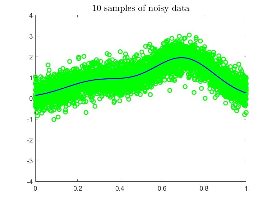

In the numerical experiment, we consider again ill-posed integral equation (4.4) with kernel
and exact solution
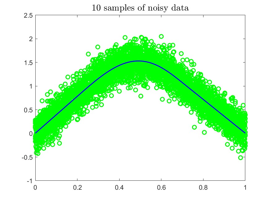
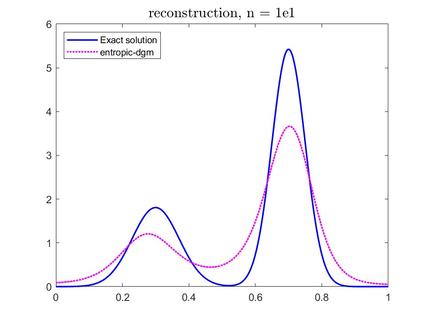
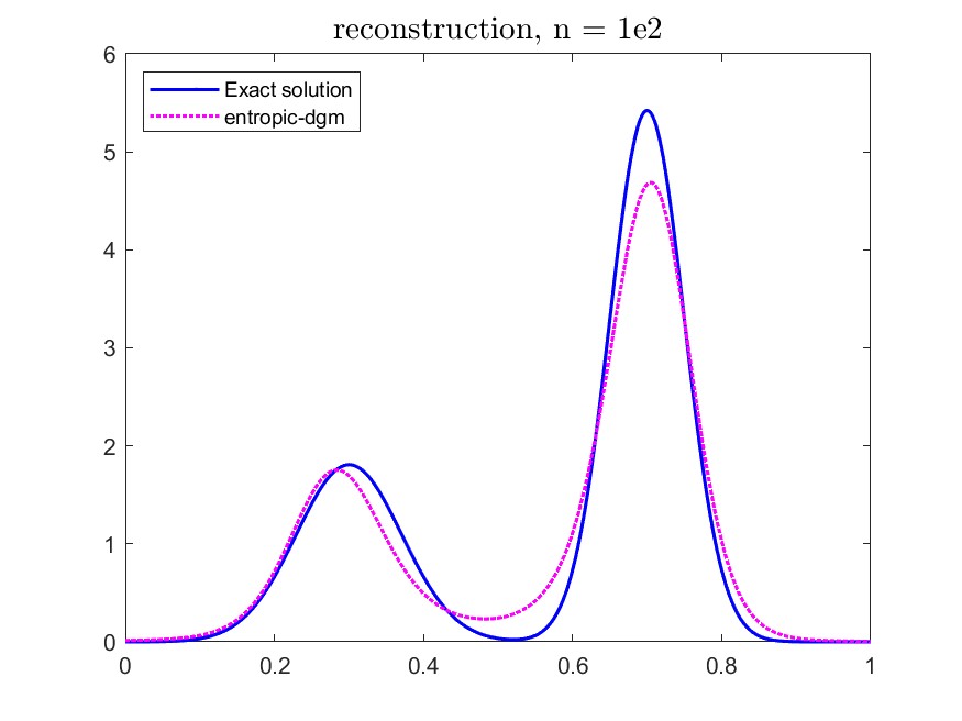
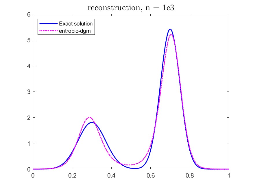
where is chosen to ensure so that is a probability density function. Clearly the integral operator is a compact linear operator from to . To perform numerical simulations, we divide into subintervals of equal length and approximate integrals by the trapezoidal rule. In Figure 3, we plot the exact data (the blue one) and the noisy data (10 samples, green circle); these noisy data are produced from the exact data by adding independent Gaussian noise in with .
| n | Iteration numbers | Relative error | Emergency stops |
|---|---|---|---|
| (in average) | |||
| 51 | 4.2691e-01 | 2 | |
| 161 | 1.7945e-01 | 0 | |
| 370 | 1.0920e-01 | 0 | |
| 1142 | 9.7181e-02 | 0 | |
| 3418 | 9.6206e-02 | 0 |
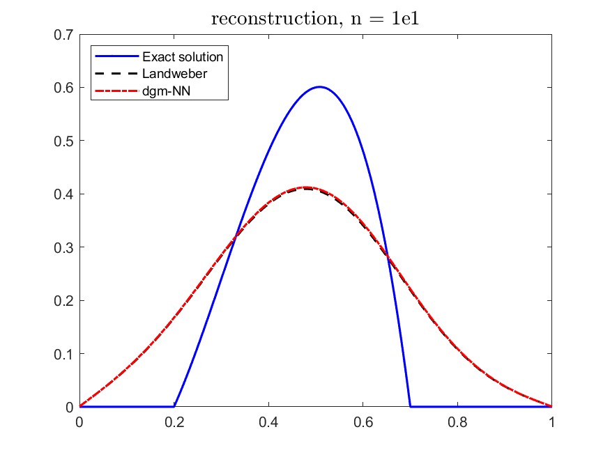
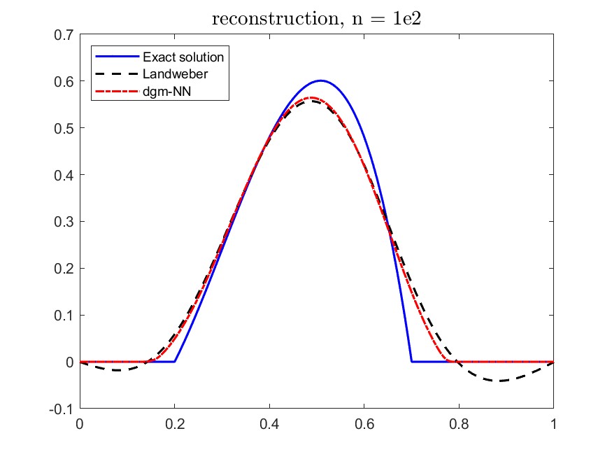
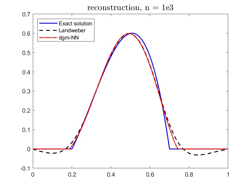
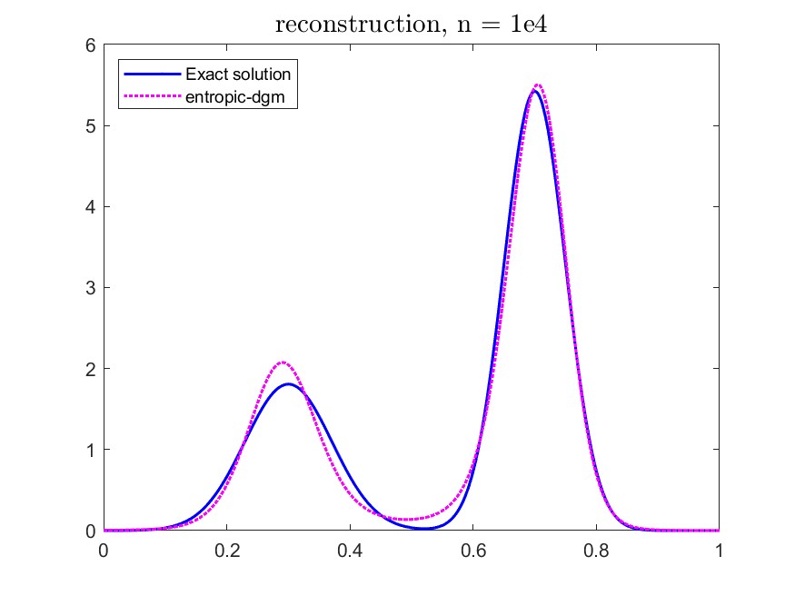
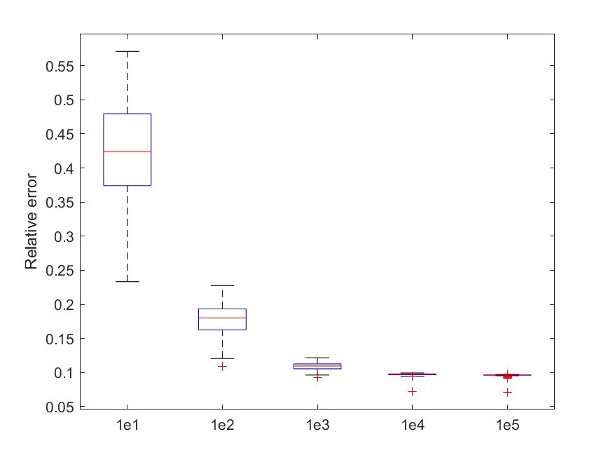
When implementing the method (4.9), we use the step-size and terminate the iteration by Rule 3.8 with and given by (3.14) with . We perform the numerical computation for several different sample sizes each is ran by 200 simulations. The reconstruction results in average are plotted in Figure 3. In Table 2 we report further computational results, including the averaged number of iterations, the relative error in average, and the utilized number of emergence stops. We also present the boxplots of the relative errors for 200 simulations in Figure 4. The results indicate that, when sample size increases, the relative error is reduced and more accurate reconstruction result can be produced.
Example 4.3.
In this example we consider using the method (1.5) to reconstruct sparse solutions for ill-posed problems , where is a bounded linear operator and is a bounded domain. For this purpose, we take to be a strongly convex perturbation of , i.e.
where is a large number. The method (1.5) then becomes
| (4.10) | ||||
where is the average of a sequence of unbiased independent identically distributed noisy data , , of the exact data .
For numerical simulations we consider determining the initial data in the time fractional diffusion equation
from the measurement of at a fixed later time , where , , and denotes the Caputo fractional derivative
with denoting the Gamma function. The mapping from to is a compact linear operator . Time fractional diffusion equations occur naturally in anomalous diffusion in which the variance of the process behaves like a non-integer power of time ([31]), sharply contrast to the classical normal diffusion which is governed by the heat equation.
To solve this inverse problem numerically, we discretize by taking grid points , and write for and for . Let . Then, by the finite difference approximation of , the diffusion equation becomes
| (4.11) | ||||
It turns out that the solution of (4.11) has the form
where each satisfies the fractional ordinary differential equation
Let and denote the discrete sine transform and the inverse disrete sine transform defined respectively by
for any matrix . Then we have and thus , where denotes the Mittag-Leffler function
Consequently
for . If we define the transform by , then . Let . Then can be determined by solving , where .


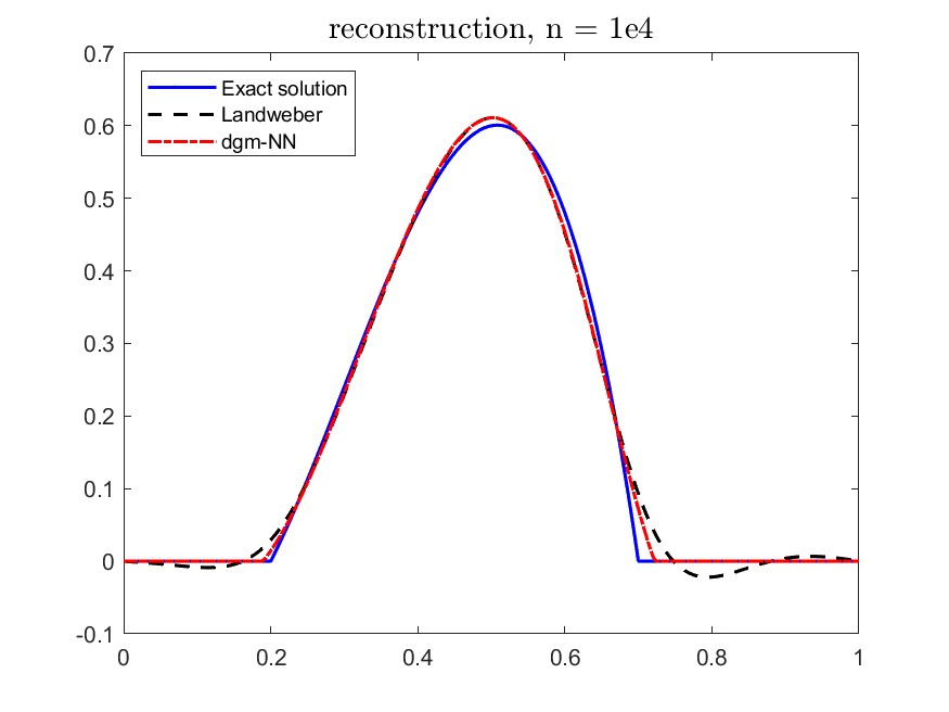
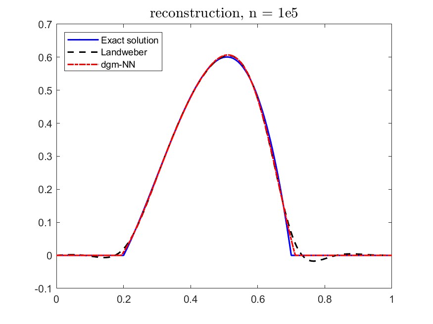
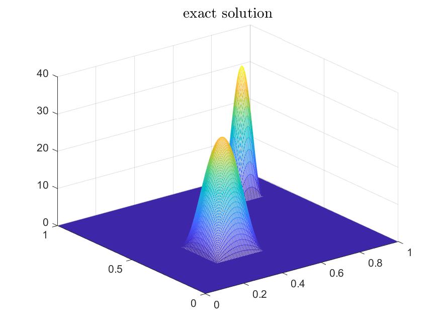
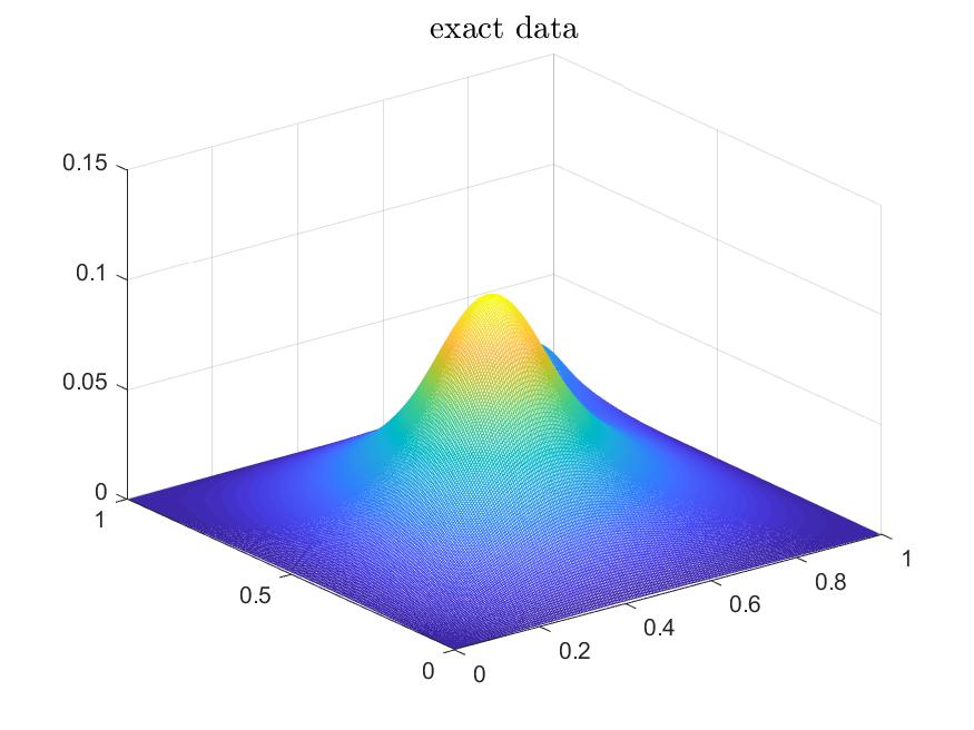
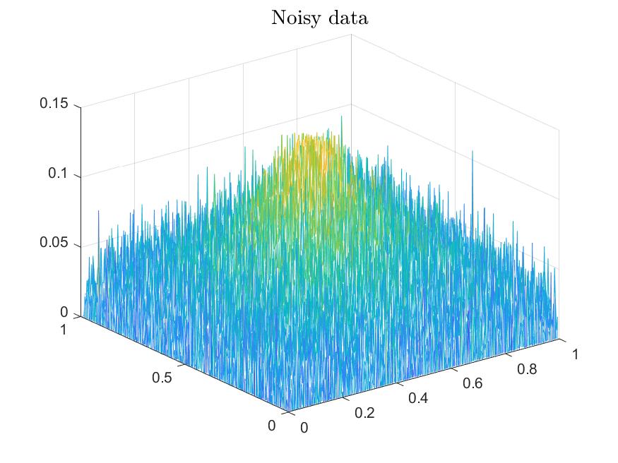
In our numerical simulation, we assume the sought solution is sparse and consider on an equidistant grid of points. The sought solution and the corresponding exact data are plotted in Figure 5 (the left and middle ones). To reconstruct , we use multiple repeated measurement data of different sample sizes which are generated from by adding independent Gaussian noise with ; one sample of measurement data is plotted in Figure 5 (the right one).
| n | Iteration numbers | Relative error | Emergency stops |
|---|---|---|---|
| (in average) | |||
| 174 | 5.9865e-01 | 0 | |
| 458 | 3.8077e-01 | 0 | |
| 933 | 1.7786e-01 | 0 | |
| 1821 | 1.1831e-01 | 0 |
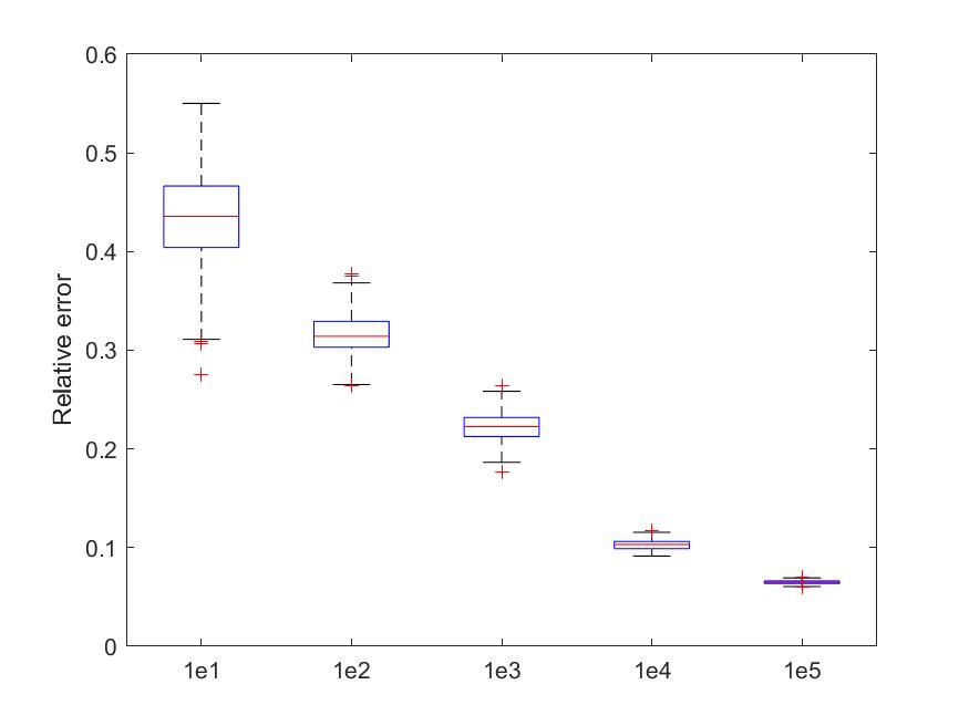
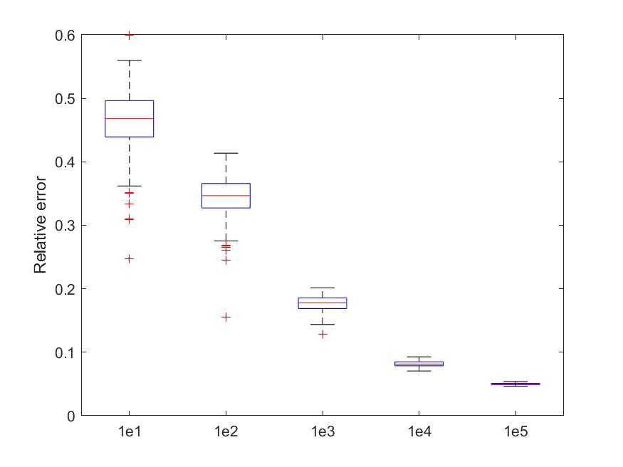
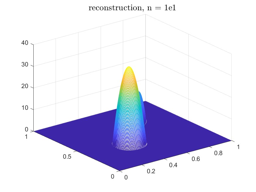
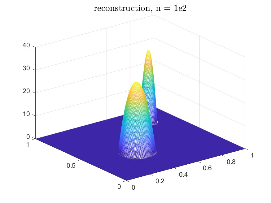
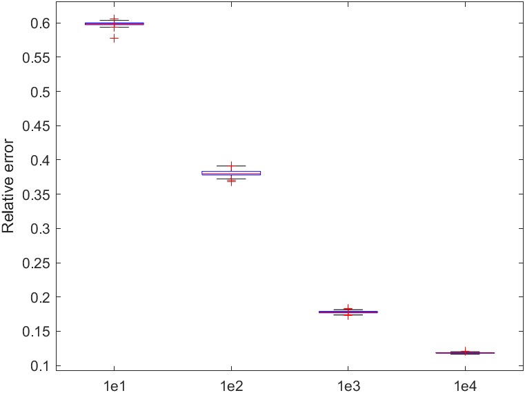
When applying the method (4.10), we take and use the step-size . The iteration is terminated by Rule 3.8 with and given by (3.14); where . The reconstruction results for several different sample sizes are plotted in Figure 6, each is based on the average of 200 runs. In Table 2 we report the average number of iterations, the average relative errors, and the number of emergency stops. Furthermore, we present the boxplots of the relative errors in Figure 7. All these result demonstrate that the proposed method can give satisfactory reconstruction results when the sample size increases and the sparsity of the sought solution can be captured well.
Example 4.4.
In this final example we consider using the method (1.5) to reconstruct piecewise constant solutions. We consider again the equation (4.4) with the kernel given by (4.7) and assume that the sought solution is piecewise constant. By dividing into subintervals of equal length and approximating integrals by the trapezoidal rule, we have a discrete ill-posed problem , where is a matrix. We use the model
| (4.12) |
where denotes the discrete gradient operator and is a large positive number. Thus, is a strongly convex perturbation of the total variation . If we apply the method (1.5) to (4.12) directly, we need to solve a minimization problem related to to obtain at each iteration. This can make the algorithm time-consuming since those minimization problems can not be solved explicitly.
To circumvent this difficulty, by introducing we reformulate (4.12) as
| (4.13) |
where
Since is strongly convex, we may apply the method (1.5) to (4.13) to obtain the iteration scheme
Since and can be given explicitly, this leads to the following algorithm
| (4.14) | ||||
| n | Iteration numbers | Relative error | Emergency stops |
|---|---|---|---|
| (in average) | |||
| 1109 | 3.5812e-01 | 10 | |
| 17877 | 2.2729e-01 | 70 | |
| 64078 | 1.7208e-01 | 0 | |
| 242623 | 1.3263e-01 | 0 | |
| 675068 | 1.0761e-01 | 0 |
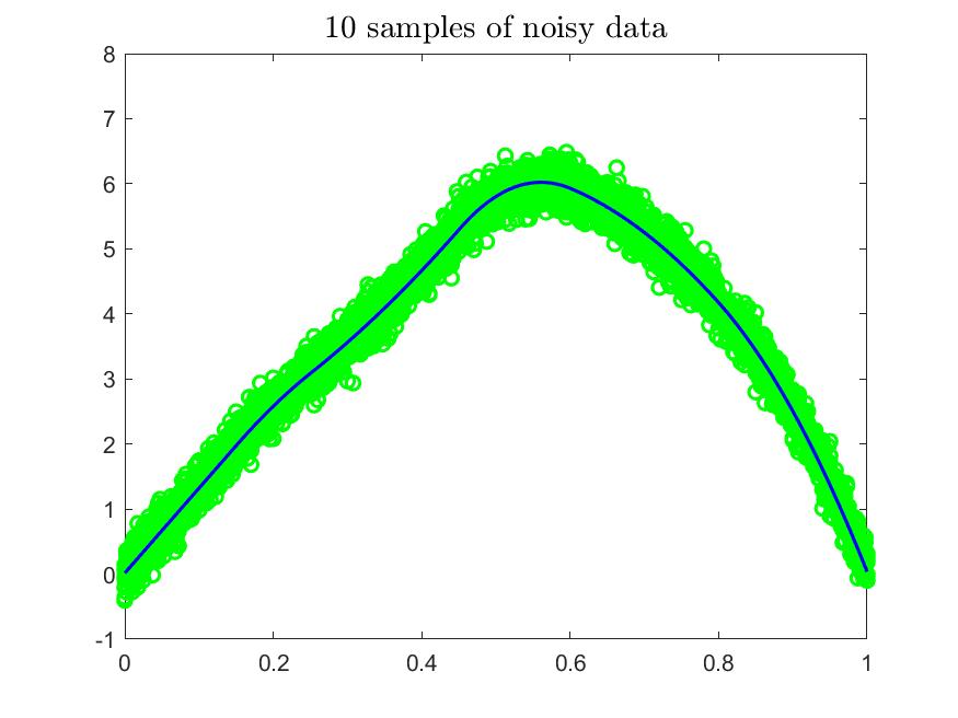
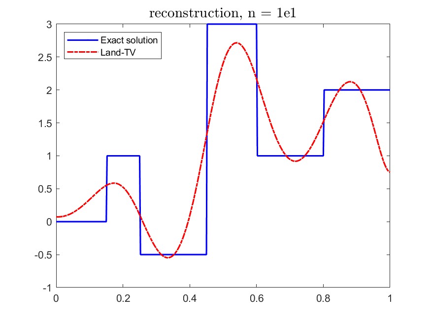
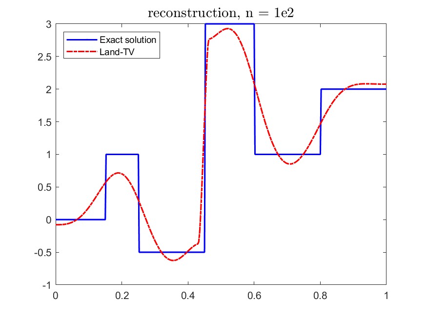
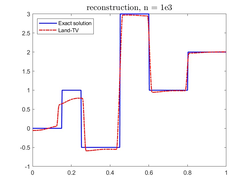
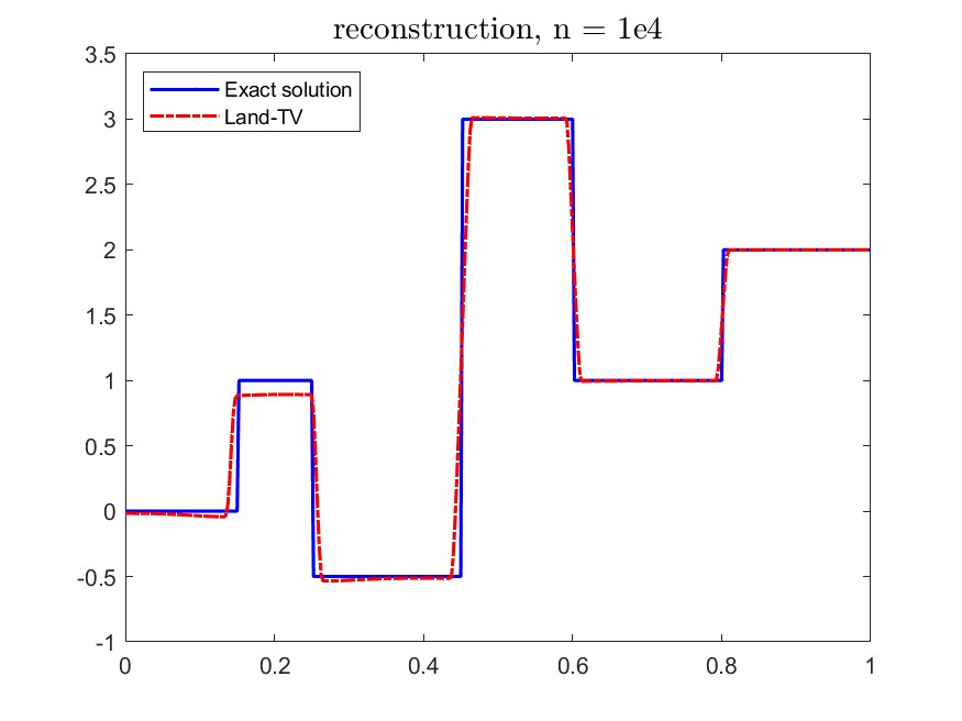
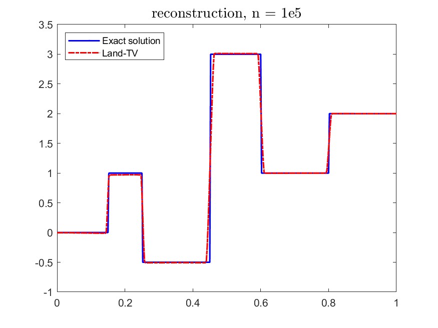
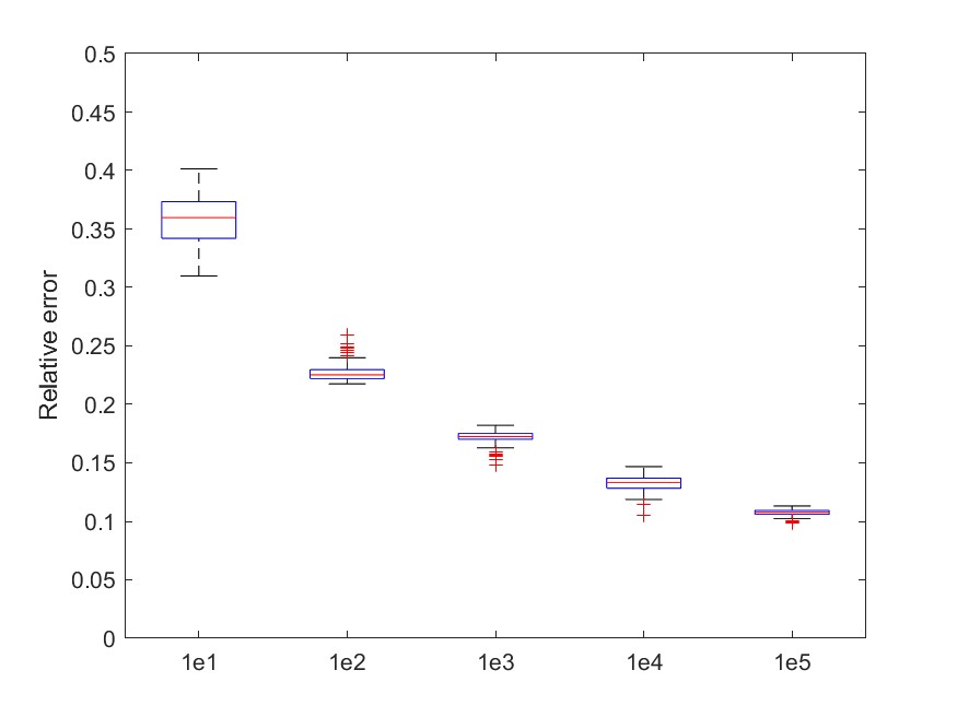
In our numerical experiments, the sought solution is piecewise constant, whose graph together with the exact data is plotted in Figure 8 in blue. In order to apply the method (4.14), we use multiple repeated measurement data of several different sample sizes corrupted by independent Gaussian noise with and let be the average of these data; 10 samples of these measurement data are plotted in Figure 8 in green. The step-size in (4.14) is chosen to be . In order to enhance the effect of total variation in reconstruction, we take . The method is terminated by Rule 3.8 adapted to (4.13) with and given by (3.14), where . For each sample size, we run 200 simulations and the reconstruction results in average are plotted in Figure 8 in red. In Table 4 we report further numerical results including the average number of iterations, the relative error in average, and the number of emergency stops used. The boxplot of the relative error is presented in Figure 9. These results clearly demonstrate that the proposed method converges and more and more satisfactory reconstruction results can be obtained when the sample size increases.
References
- [1] A. B. Bakushinskii, Remarks on choosing a regularization parameter using the quasioptimality and ratio criterion, Comp. Math. Math. Phys., 24 (1984), 181–182.
- [2] A. Beck and M. Teboulle, A fast dual proximal gradient algorithm for convex minimization and applications, Oper. Res. Lett., 42 (2014), no. 1, 1–6.
- [3] J. M. Borwein and C. S. Lewis, Convergence of best entropy estimates, SIAM J. Optim., 1 (1991), pp. 191–205.
- [4] R. Boţ and T. Hein, Iterative regularization with a geeral penalty term – theory and applications to and TV regularization, Inverse Problems, 28 (2012), 104010.
- [5] M. Burger, E. Resmerita and M. Benning, An entropic Landweber method for linear ill-posed problems, Inverse Problems, 36 (2019), 015009.
- [6] D. H. Chen, D. Jiang, I. Yousept and J. Zou, Variational source conditions for inverse Robin and flux problems by partial measurements, Inverse Probl. Imaging, 16 (2022), no. 2, 283–304.
- [7] D. H. Chen and I. Yousept, Variational source condition for ill-posed backward nonlinear Maxwell’s equations, Inverse Problem, 35 (2019), 025001.
- [8] H. W. Engl, M. Hanke and A. Neubauer, Regularization of Inverse Problems, Kluwer, Dordrecht, 1996.
- [9] J. Flemming,Existence of variational source conditions for nonlinear inverse problems in Banach spaces, J. Inverse Ill-posed Problems, 26 (2018), no. 2, 277–286.
- [10] K. Frick and O. Scherzer,Regularization of ill-posed linear equations by the non-stationary augmented Lagrangian method, J. Integral Equ. Appl., 22 (2010), no. 2, 217–257.
- [11] M. Grasmair, Source conditions for non-quadratic Tikhonov regularization, Numer. Funct. Anal. Optim., 41 (2020), no. 11, 1352–1372.
- [12] P. C. Hansen and D. P. O. Leary, The use of the L-curve in the regularization of discrete ill-posed problems, SIAM J. Sci. Comput., 14 1487–503.
- [13] B. Harrach, T. Jahn and R. Potthast, Beyond the Bakushinkii veto: regularising linear inverse problems without knowing the noise distribution, Numer. Math., 145 (2020), no. 3, 581–603.
- [14] U. Hassan and M. S. Anwar, Reducing noise by repetition: introduction to signal averaging. Eur. J. Phys., 31 (2010), no. 3, 453–465.
- [15] B. Hofmann, B. Kaltenbacher, C. Pöschl and O. Scherzer,A convergence rates result for Tikhonov regularization in Banach spaces with non-smooth operators, Inverse Problems, 23 (2007), 987–1010.
- [16] B. Hofmann and P. Mathé, Parameter choice under variational inequalities, Inverse Problems, 28 (2012), 104006.
- [17] 24. T. Hohage and F. Weidling, Verification of a variational source condition for acoustic inverse medium scattering problems, Inverse Problems 31 (2015), no. 7, 075006.
- [18] T. Hohage and F. Weilding, Variational source condition and stability estimates for inverse electromagnetic medium scattering problems, Inverse Probl. Imaging, 11 (2017), 203–220.
- [19] T. Hohage and F. Weidling, Characterizations of variational source conditions, converse results, and maxisets of spectral regularization methods, SIAM J. Numer. Anal., 55 (2017), no. 2, 598–620.
- [20] Q. Jin, Hanke-Raus heuristic rule for variational regularization in Banach spaces, Inverse Problems, 32 (2016), no. 8, 085008.
- [21] Q. Jin, On a heuristic stopping rule for the regularization of inverse problems by the augmented Lagrangian method, Numer. Math., 136 (2017), no. 4, 973–992.
- [22] Q. Jin, Convergence rates of a dual gradient method for constrained linear ill-posed problems, Numer. Math., 151 (2022), no. 4, 841–871.
- [23] Q. Jin and L. Stals, Nonstationary iterated Tikhonov regularization for ill-posed problems in Banach spaces, Inverse Problems, 28 (2012), no. 10, 104011.
- [24] Q. Jin and W. Wang, Landweber iteration of Kaczmarz type with general non-smooth convex penalty functionals, Inverse Problems, 29 (2013), no. 8, 085011, 22 pp.
- [25] S. Kindermann and A. Neubauer, On the convergence of the quasioptimality criterion for (iterated) Tikhonov regularization, Inverse Probl. Imaging, 2 (2008), 291–299.
- [26] S. Kindermann and K. Raik, Convergence of heuristic parameter choice rules for convex Tikhonov regularization, SIAM J. Numer. Anal., 58 (2020), no. 3, 1773–1800.
- [27] J. Kivinen and M. K. Warmuth, Exponentiated gradient versus gradient descent for linear predictors, Information and Computation, 132 (1997), no. 1, 1–63.
- [28] M. Ledoux and M. Talagrand, Probability in Banach Spaces: Isoperimetry and Processes, vol. 23. Springer, Berlin, 1991.
- [29] R. G. Lyons, Understanding Digital Signal Processing, 3/E. Pearson Education India, Chennai, 2004.
- [30] S. Nemirovski and D. B. Yudin, Problem Complexity and Method Efficiency in Optimization, Wiley, New York, 1983.
- [31] I. Podlubny, Fractional Differential Equations, San Diego, CA: Academic, 1999.
- [32] T. Schuster, B. Kaltenbacher, B. Hofmann and K. S. Kazimierski,Regularization Methods in Banach Spaces, Radon Series on Computational and Applied Mathematics 10 Walter de Gruyter, Berlin 2012.
- [33] P. Tseng, Applications of a splitting algorithm to decomposition in convex programming and variational inequalities, SIAM J. Control Optim., 29 (1991), no. 1, 119–138.
- [34] H. Uzawa, Iterative methods for concave programming, in: Studies in Linear and Nonlinear Programming, 1958, pp. 154–165.
- [35] W. van Drongelen, Signal Processing for Neuroscientists, 2nd edition, Academic Press, 2018.
- [36] C. Zălinscu, Convex Analysis in General Vector Spaces, World Scientific Publishing Co., Inc., River Edge, New Jersey, 2002.