Holographic entanglement entropy for relativistic hydrodynamic flows

Abstract

We study the behaviour of holographic entanglement entropy (HEE) in near equilibrium thermal states which are macroscopically described by conformal relativistic hydrodynamic flows dual to dynamical black brane geometries. We compute HEE for strip-shaped subsystems in boundary dimensions $d=2,3,4$, which provides us with general qualitative inferences on the interplay between fluid flows and entanglement dynamics. At first, we consider the zeroth order in hydrodynamic derivative expansion, holographically described by stationary boosted black branes. Working non-perturbatively in fluid velocity, we find that, as the fluid velocity approaches its relativistic upper limit, the UV regulated HEE exhibits a divergence at arbitrary temperature. Also, the holographic mutual information between two relatively close subsystems vanishes at some critical fluid velocity and remains zero beyond it. We then compute HEE in an excited state of the fluid in the presence of the sound mode. As a simplified setup, we first work with non-dissipative dynamics in $d=2$, where the time evolution of HEE is studied in the presence of the sound mode and a propagating pressure pulse. In $d=4$, working upto first order in derivative expansion, we find that dissipative sound modes produce an additional dynamical UV divergence which is subleading compared to the ‘area law divergence’. No such divergence is observed for dissipative sound mode in $d=3$.

1 Introduction

The translationally invariant macroscopic thermal dynamics of a quantum field theoretic system is believed to be captured by a set of effective hydrodynamic degrees of freedom. The theory governing these hydrodynamic variables is primarily based on the underlying symmetries, which makes its applicability significantly universal. In the hydrodynamic description, the relevant microscopic information is packaged into a few parameters - the transport coefficients. The fluid variables capture the near equilibrium dynamics very efficiently, while the corresponding microscopic dynamics is extremely complex. The intricate interplay between the macro and micro dynamics usually provides us with enourmous insights into a physical system, but usually is a difficult question to address. The difficulty mainly arises due to the intractability of the microscopic degrees of freedom in such a situation. The fluid-gravity correspondence Bhattacharyya:2007vjd provides us with a very special setting where a complete picture is provided and the transport coefficients are determined from the dynamics of a dual black brane. In this picture, the various length scales of the hydrodynamic system are encoded in a holographic direction.

The fluid-gravity correspondence maps the dynamics of a $d$ dimensional conformal relativistic fluid to that of a AdS_(d+1) black brane. The microscopic description of this holographic fluid is provided by a strongly coupled conformal gauge theory. The black brane has a complete knowledge of this strongly coupled microscopics. This is why, all the hydrodynamic transport coefficients can be computed from the black brane geometry, in a regime where a direct field theoretic calculation is intractable. Similarly, the holographic geometry can be used to extract other microscopic information about the near-equilibrium thermal states. Particularly, the entanglement structure of these underlying quantum field theoretic states, which are evolving towards equilibrium, is significantly interesting. An excellent measure of this entanglement is provided by the holographic entanglement entropy (HEE) Ryu:2006bv ; Ryu:2006ef ; Hubeny:2007xt ; Nishioka:2009un ; Rangamani:2016dms ; Headrick:2019eth . In this paper, our objective is to apply the holographic dictionary to study the dynamics of HEE for the states whose macrodynamics corresponds to specific hydrodynamic flows.

In order to compute entanglement entropy in a continuum field theoretic set up, we first choose a subsystem $A$, usually taken to be a space-like sub-region on a chosen time-slice. The entanglement entropy of a given state, is then given by the Von Neumann entropy of the reduced density matrix obtained by integrating out the degrees of freedom outside $A$. The knowledge of this entanglement entropy for various subsystems provides us with enourmous quantum information about the underlying state. Holographically, this entanglement entropy is computed by the celebrated Ryu-Takayanagi formula Ryu:2006bv ; Ryu:2006ef , which was generalized to a more general covariant form in Hubeny:2007xt . In this prescription, the HEE for $A$ is given by

$$S_{A}=\frac{A_{\Gamma}}{4G_{N}},$$ (1)

where $A_{\Gamma}$ is the area of the co-dimension 2 surface homologous to $A$ which has been extremized on the bulk geometry dual to the the field theoretic boundary state. The subscript $\Gamma$ refers to this extremal surface. In our work here, using the fluid-gravity map, we will explicitly write down the geometries dual to specific hydrodynamic configurations. Subsequently, we shall compute the area of the extremal surface in these geometries to obtain HEE ($S_{A}$) for the hydrodynamic states. For the subsystem $A$, we choose a strip-shaped sub-region on a canonical time slice of the AdS boundary. Our choice of subsystem is time-independent, while the underlying state is a fluctuating fluid configuration (see fig.1).

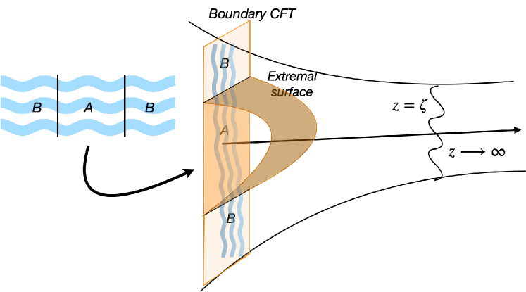
Figure 1: A Schematic representation of the strip-shaped subsystem $A$ on a canonical time-slice of the AdS boundary for which holographic entanglement is to be computed. The underlying state is a fluctuating fluid configuration in our set-up.

In this paper, we shall primarily focus on two varieties of fluid configurations. In the first case, we shall consider steady state flows where the fluid is moving with a constant velocity (see section 2). The computation of HEE for such thermal systems has been attempted by several authors in the recent past Fischler:2012uv ; Fischler:2012ca ; Bhattacharya:2013bna ; Blanco:2013joa ; Mishra:2015cpa ; Mishra:2016yor ; Bhatta:2019eog ; Maulik:2020tzm ; ChowdhuryRoy:2022dgo . However, in all these earlier works, some simplifying assumption have been made, and therefore, a thorough analysis, particularly in the regime where the fluid velocity approaches its relativistic upper bound, seems to be missing so far. For this steady state case, apart from HEE, we also compute the holographic mutual information between two non-overlapping strip-shaped subsystems. Among various other results, we find that there is a critical fluid velocity beyond which mutual information vanishes due to an exchange of dominance of extremal surfaces. This is similar to the ‘disentangling transition’ previously observed in Headrick:2010zt ; Fischler:2012uv , where the abrupt vanishing of mutual information was observed as the separation between the two subsystems in question exceeded a certain critical value . In this paper, we observe such a ‘disentangling transition’ taking place as a function of the fluid velocity. This we believe, is a new and important result, which was not possible to obtain without the non-perturbative approach of our paper.

In another case, we consider fluid configurations where a propagating sound wave have been set up with some initial conditions. We then proceed to study the change in HEE produced due to such fluid fluctuations in the linearized approximation, assuming a small amplitude of the excitation (see section 3). Since, sound waves constitute one of the basic fluid excitations, it is interesting to understand the HEE dynamics associated with it. In $d=2$ the sound mode is non-dissipative, while in higher dimensions these fluctuations dissipate away to equilibrium. In the latter case, we aim to capture the time-evolution of HEE as the fluid settles back to equilibrium. In $d=2$ where the sound mode is non-dissipative, we can superpose them to constitute a pressure or energy density pulse. In this case, we study how HEE evolves with time as the pulse passes across the subsystem. Our investigation here is reminiscent of Narayan:2012ks where HEE has been computed in the AdS plane wave geometry with an energy flux flowing through the subsystem. We are also inspired by the body of work on the study of HEE following quantum quenches (see for instance Nozaki:2013wia ; Rangamani:2015agy ; Jahn:2017xsg ). In fact, we may consider our fluid dynamical set-up to be a thermal state which has been quenched by a macroscopic observable associated with the energy-momentum tensor, and we study the subsequent late time evolution of HEE.

In our work here, we employ a mixture of analytical and numerical techniques. In particular, most of our results in $d=2$ is analytical. We use this analytical result to optimize our numerical procedure, which are then applied to $d=3,4$. The qualitative inferences which we draw from our results in $d=2,3,4$ may be straightforwardly generalized to higher dimensions.

Summary of results

Before proceeding to the details, let us summarize the important new results of our paper below. In this paper we investigate the behaviour of entanglement entropy in a class of conformal fluid states, using holographic techniques, for a strip like subsystem.

• We compute HEE for boosted black holes in $d+1$ ($d=2,3,4$), viewed as holographic geometries dual to fluids moving with a constant velocity. Our subsystem lies on a ‘canonical time slice’ and its size is fixed as we vary the fluid parameters. Our calculation is performed without making any assumption on temperature or velocity parameter. All earlier studies of this system had made some simplifying assumption about these parameters and lifting those assumptions is a new aspect of our study. In particular, we curiously observe that the regulated HEE diverges as the fluid velocity approaches its relativisitc upper bound ($v\rightarrow 1$) (see fig.4 and fig.6). See section 2 for more details.

• For the constant velocity fluid flows, we also compute holographic mutual information. We find that this quantity undergoes an abrupt ‘disentangling’ transition for some critical velocity for any separation between the subsystems (see fig.5 and fig.7). This critical velocity tends to 1 as the separation between the subsystem tends to zero. The existence of this critical velocity is a new and interesting result. See section 2.2.2 and section 2.3 for more details.

• For holographic fluids in d=2, we have studied the time dependence of HEE as a non-dissipative propagating pressure pulse passes through the demarcated subsystem. The geometric dual to this pressure (or energy) pulse is an exact solution to the bulk Einstein equations. We find that HEE has a curious dip when the pulse enters the subsystem, followed by an expected rise and plateau while the pulse resides inside the subsystem (see fig.10). We report these results in section 3.2.

• For holographic fluids in $d=3,4$, we study the behaviour of HEE in the presence of a dissipative sound mode. In this case HEE has the usual expected decay closely following the damping of the sound mode. However, surprisingly, we find that in d=4, there is an additional UV divergence which is subdominant compared to usual area law (see (72)). We present the details of these results in section 3.3.

2 Entanglement in steady state relativistic fluid flows

2.1 General Procedure

Before proceeding with the hydrodynamic excitations, we would like to consider the simple steady state case, when the fluid is moving with a constant velocity. More precisely, we consider a relativistic conformal fluid, with a constant velocity, in a flat Minkowski background with

$$\eta_{\mu\nu}=\text{Diag}\{-1,1,1,\dots\}.$$

Holographically, this fluid configuration is described by a bulk metric of a boosted black brane, which in $d+1$ dimensional Schwarzschild coordinates , takes the form

$$ds^{2}_{\text{Sch}}=\frac{1}{z^{2}}\left(-dt^{2}+dx^{2}+g(z)\big{(}dt~{}-~{}v~{}dx\big{)}^{2}+\frac{dz^{2}}{f(z)}+\sum_{i=1}^{d-2}dy_{i}^{2}\right)$$ (2)

where

$$f(z)=1-\left(\frac{z}{\zeta}\right)^{d},~{}~{}g(z)=\gamma^{2}\left(\frac{z}{\zeta}\right)^{d},~{}~{}\gamma=\frac{1}{\sqrt{1-v^{2}}}.$$

Here, $0\leq v\leq 1$ is the boost parameter which is identified with the fluid velocity. Also, the AdS boundary is reached in the limit $z\rightarrow 0$. We denote the horizon radius with $\zeta$, which is related to the temperature of the black brane as

$$T=\frac{d}{4\pi\zeta}\equiv\frac{1}{\beta}.$$ (3)

This is also identified with the steady state temperature of the fluid.

The equations of hydrodynamics in steady state is provided by the conservation of the energy-momentum tensor, which has the following constitutive relations

$$T^{\mu\nu}=\mathcal{E}(T)u^{\mu}u^{\nu}+\mathcal{P}(T)P^{\mu\nu}+\mathcal{O}(\partial),$$ (4)

where $P^{\mu\nu}=\eta^{\mu\nu}+u^{\mu}u^{\nu}$ is the projector orthogonal to the fluid velocity $u^{\mu}$, $\mathcal{E}(T)$ and $\mathcal{P}(T)$ are respectively the energy and pressure densities, while $\mathcal{O}(\partial)$ represents higher derivative corrections to this perfect fluid form. In steady state, the temperature and fluid velocity are constants over space-time, implying that all the higher derivative terms vanish. Also, for such a steady state it is immediately clear that the fluid variables satisfy the conservation equations $\partial_{\mu}T^{\mu\nu}=0$. The form of the energy momentum tensor (4) follows from the boosted AdS black brane (2), via the AdS-CFT dictionary. The duality also determines the precise functional forms

$$\mathcal{P}(T)=\frac{1}{16\pi G_{N}}\left(\frac{4\pi T}{d}\right)^{d},~{}~{}\mathcal{E}(T)=(d-1)\mathcal{P}(T)$$ (5)

On the boundary of the boosted black brane, we choose a strip like subsystem ($A$) on a canonical time-slice and we wish to quantify the entanglement of $A$ with the region outside the strip. The underlying fluid is moving with a constant velocity in some given direction (see fig.1 for a schematic of the situation).

For zero boost ($v=0$), the HEE for black branes in arbitrary dimensions have been computed in Fischler:2012uv ; Fischler:2012ca ; Bhattacharya:2013bna . The extension of this analysis to boosted black branes have been attempted in several papers earlier Blanco:2013joa ; Mishra:2015cpa ; Mishra:2016yor ; Bhatta:2019eog ; Maulik:2020tzm ; ChowdhuryRoy:2022dgo . However, in all these papers some simplifying approximations have been employed, such as small boost in Mishra:2015cpa ; Mishra:2016yor ; Bhatta:2019eog , or small temperature Blanco:2013joa . To our knowledge, a complete computation of HEE for arbitrary boost and arbitrary temperature seems to be missing in the literature. This subsection aims to perform a thorough analysis of this situation, particularly focusing on the situation when the fluid velocity approaches its relativistic upper bound ($v\rightarrow 1$) at an arbitrary background temperature.

As pointed out in Blanco:2013joa , for a non-perturbative HEE computation in this scenario, the extremal surface is not expected to lie on a bulk time-slice. Therefore, even if we are using Schwarzschild coordinates (2), for the boosted case, we must employ the covariant protocol of Hubeny:2007xt .

Here, we shall consider a strip-shaped subsystem in a $d$ dimensional space-time. The symmetries of such a strip-like subsystem simplify some of the calculations significantly. From the boundary point of view, there are two special spatial directions in this set-up. The short edge of the strip is directed along some spatial direction, while the boosted fluid may be flowing in any other independent direction. The result of HEE is expected to depend on the angle between these two vectors. But again for the sake of simplicity, in this paper, we will assume these directions to be collinear, i.e. the short edge of the strip is extended along the same direction as the boost. With this in mind, the embedding ansatz for the extremal surface, which is a co-dimension 2 surface homologous to our strip like subsystem on the boundary (see fig.1), is taken to be

$$\Gamma:~{}x=x(\phi,\tilde{y}_{i}),~{}t=t(\phi,\tilde{y}_{i}),~{}z=z_{\star}\cos\phi,~{}y_{i}=\tilde{y}_{i}.$$ (6)

In other words, the world-volume of our co-dimension 2 extremal surface is parameterized by $\phi$ and $\tilde{y}_{i}$. The $\phi$-coordinate on the world-volume takes values between $-\pi/2\leq\phi\leq\pi/2$, and $z_{\star}(<\zeta)$ is the turning point of the extremal surface, which will be determined in terms of the width $\ell$ of the strip on the boundary. Further, on the boundary, to regulate the infinite volume arising due to the long sides of the strip, we will consider the $\tilde{y}_{i}$ coordinates to be bounded

$$-\frac{L}{2}\leq\tilde{y}_{i}\leq\frac{L}{2},~{}~{}i=1,2\cdots d-2,~{}~{}\text{with}~{}~{}L\rightarrow\infty.$$

Now, since the boost is along the $x$-direction (along the short-edge of the strip) (2), we retain translation invariance along the $\tilde{y}_{i}$-directions. Thus, we need to solve for two functions of one variable, $x(\phi)$ and $t(\phi)$. The area functional of $\Gamma$, to be extremized, is given by

$$A_{\Gamma}=L^{d-2}\int d\phi\left(\frac{1}{z_{\star}\cos\phi}\right)^{d-1}\left[-(1-g)t^{\prime 2}+(1+v^{2}g)x^{\prime 2}-2vgt^{\prime}x^{\prime}+\frac{z_{\star}^{2}\sin^{2}\phi}{f}\right]^{\frac{1}{2}}.$$ (7)

where $x^{\prime}$ and $t^{\prime}$ denotes derivatives of these functions with respect to $\phi$. Here, the factor of $L^{d-2}$ arises due to the integrals over the $\tilde{y}_{i}$ coordinates on the world-volume of the extremal surface. Also, in (7) $g=g(z_{\star}\cos\phi)$, and $f=f(z_{\star}\cos\phi)$   and their functional forms are given in (2). The equation of motion for $x(\phi)$ and $t(\phi)$ which follows from the extremization of $A_{\Gamma}$ is given by

$$\begin{split}&\frac{\partial}{\partial\phi}\left(\frac{(1-g)t^{\prime}+vgx^{\prime}}{\mathcal{K}\left(\phi,x(\phi),t(\phi)\right)}\right)=0,~{}~{}~{}\frac{\partial}{\partial\phi}\left(\frac{(1+v^{2}g)x^{\prime}-vgt^{\prime}}{\mathcal{K}\left(\phi,x(\phi),t(\phi)\right)}\right)=0,~{}~{}\text{where,}\\ &\mathcal{K}\left(\phi,x(\phi),t(\phi)\right)=(z_{\star}\cos\phi)^{d-1}\left[-(1-g)t^{\prime 2}+(1+v^{2}g)x^{\prime 2}-2vgt^{\prime}x^{\prime}+\frac{z_{\star}^{2}\sin^{2}\phi}{f}\right]^{\frac{1}{2}}.\end{split}$$ (8)

We now have to solve these equations (8), with the following boundary conditions

$$x(-\pi/2)=-\frac{\ell}{2},~{}x(\pi/2)=\frac{\ell}{2},~{}~{}t(-\pi/2)=0=t(\pi/2).$$ (9)

Since, we are dealing with a stationary scenario, we expect the HEE to be independent of time. Hence without any loss of generality we have chosen the boundary time slice at $t_{b}=0$.

The equations (8), (9) is difficult to solve analytically. Therefore, we have to resort to numerical analysis for computing the area of the extremal surface.

In the absence of boost ($v=0$), $t(\phi)=\text{constant}$ is a solution to the equations (8). This implies that, in the unboosted case, if we use Schwarzschild coordinates, the extremal surface always lies on a constant time-slice throughout the bulk. This, however, is not the case in the presence of boost, even if we work in Schwarzschild coordinates.

Extremal surface reparameterization: $\phi\rightarrow z$

It is often practically useful to consider the embedding of the extremal surface such that the AdS-radial coordiate $z$ is identified with one of the world-volume coordinates. With such a choice, the embedding equations for the strip-subsystem would read

$$\Gamma:~{}x=x(z),~{}t=t(z),~{}z=z,~{}y_{i}=\tilde{y}_{i},$$ (10)

with the equations of motion (8) being minimally modified to

$$\begin{split}&\frac{\partial}{\partial z}\left(\frac{(1-g)t^{\prime}+vgx^{\prime}}{\mathcal{K}\left(z,x(z),t(z)\right)}\right)=0,~{}~{}~{}\frac{\partial}{\partial z}\left(\frac{(1+v^{2}g)x^{\prime}-vgt^{\prime}}{\mathcal{K}\left(z,x(z),t(z)\right)}\right)=0,~{}~{}\text{where,}\\ &\mathcal{K}\left(z,x(z),t(z)\right)=z^{d-1}\left[-(1-g)t^{\prime 2}+(1+v^{2}g)x^{\prime 2}-2vgt^{\prime}x^{\prime}+\frac{1}{f}\right]^{\frac{1}{2}}.\end{split}$$ (11)

Now $x^{\prime}$ and $t^{\prime}$ denote derivatives with respect to $z$, while $f=f(z)$ and $g=g(z)$ as given in (2). In this case, the boundary conditions (9), are implemented with a minor difference. The solution to (11) has two distinct branches ($x_{\pm}(z),t_{\pm}(z)$) which are valid in the domain $z\in[z_{\star},0]$, with $z_{\star}$ being the turning point. The boundary conditions for the two roots are implemented in the following way

$$x_{\pm}(z\rightarrow 0)=\pm\frac{\ell}{2},~{}~{}t_{\pm}(z\rightarrow 0)=0,~{}~{}x^{\prime}_{\pm}(z\rightarrow z_{\star})\rightarrow\infty,~{}~{}t^{\prime}_{\pm}(z\rightarrow z_{\star})\rightarrow\infty.$$ (12)

The two branches are smoothly stiched together at the turning point $z_{\star}$ (see fig.3 for the extremal line in $d=2$).

The area functional, after this reparameterization, is given by

$$A_{\Gamma}=L^{d-2}\int\frac{dz}{z^{(d-1)}}\left[-(1-g)t^{\prime 2}+(1+v^{2}g)x^{\prime 2}+2vgt^{\prime}x^{\prime}+\frac{1}{f}\right]^{\frac{1}{2}}.$$ (13)

This area functional evaluated on the extremal surface gives the HEE by the formula (1). We shall regulate the UV divergence by removing the HEE corresponding to pure AdS

$$\mathcal{S}=\frac{A_{\Gamma}}{4G_{N}},~{}~{}\Delta\mathcal{S}=\mathcal{S}-S^{\text{vac}}\eqqcolon\frac{L^{(d-2)}}{4G_{N}}\Delta S_{E}.$$ (14)

The $\Delta S_{E}$, as defined above, will be useful for quoting our numerical results.

2.2 Fluid flows in $d=2$ dual to boosted BTZ black brane

In $1+1$D boundary, an exact expression of HEE for the steady state fluid flow dual to boosted BTZ black brane, may be obtained by a simple argument using a result available in Kusuki_2017 . After presenting this argument in section 2.2.1, we proceed directly to solve the equations (8) numerically and verify our argument. Further, in $d=2$ we can also use our analytical result to compute mutual information for configurations with constant fluid velocity, which we present in section 2.2.2.

Our numerical procedure in $d=2$, having been verified by an exact analytical result, is then straightforwardly carried over to higher dimensions in section 2.3.

2.2.1 Holographic Entanglement entropy

Analytical exact result

Let us first consider the unboosted BTZ black brane in Schwarzschild coordinates

$$ds^{2}=\frac{1}{z^{2}}\left(-f(z)dt^{2}+\frac{1}{f(z)}dz^{2}+dx^{2}\right).$$ (15)

where, $f(z)$ is given by the same function in (2) for $d=2$. This metric is dual to a static fluid configuration in $d=2$ with fluid velocity $u^{\mu}=\{-1,0\}$ and temperature given by (3).

Now, we wish to define our boundary subsystem ($A$) as the region between two space like points, say $P$ and $Q$. Without the loss of generality, we can consider the boundary points to be $P\equiv(0,0)$ and $Q\equiv(\tau,\xi)$. The HEE for this situation was worked out in Hubeny:2007xt ; Kusuki_2017 and the answer is given by

$$\mathcal{S}_{A}=\frac{c}{6}\ln\left(\frac{\beta^{2}}{\pi^{2}\epsilon_{{\text{uv}}}^{2}}\sinh\left(\frac{\pi}{\beta}\left(\xi+\tau\right)\right)\sinh\left(\frac{\pi}{\beta}\left(\xi-\tau\right)\right)\right)$$ (16)

where $\epsilon_{{\text{uv}}}$ is the ultraviolet cut-off .

Let us boost this set-up with velocity $v$, so that the fluid velocity becomes $u^{\mu}=\gamma(-1,v)$. Under this boost, the bulk BTZ metric (15) goes over to (2) (for $d=2$). Besides affecting the underlying fluid state, the boost also transforms the end points of our subsystem $P$ and $Q$. Consequently, our subsystem $A$ will now lie on a different time-slice compared to the time-slice before boosting. We wish to compute HEE for the boosted BTZ when our subsystem $A$ lies on a canonical time-slice (see footnote 4).

Figure 2: Schematic representation of the argument leading to the computation of HEE for the steady state of a $1+1$D conformal fluid, moving with a constant velocity. We start with the static fluid and find HEE for a subsystem defined by the points $P$ and $Q$ as shown in the left figure. This situation is boosted so that the system, now defined by the points $\tilde{P}$ and $\tilde{Q}$, returns back on to a canonical time slice as shown in the right figure (see footnote 4). The boosting ensures that the background fluid is moving with a constant velocity, equal to the value of the boost parameter. This procedure enables us to write down an exact expression for HEE in this case, as given by (20).

The boosted coordinates would be related to the old coordinates by the transformation

$$\tilde{t}=u^{\mu}x_{\mu}=\gamma\left(t+vx\right),~{}~{}\tilde{x}=\sqrt{x^{\nu}x^{\mu}P_{\nu\mu}}=\gamma\left(x+vt\right)\,$$ (17)

where $P_{\mu\nu}=\eta_{\mu\nu}+u_{\mu}u_{\nu}$ is the projector orthogonal to $u^{\mu}$. Now, prior to boosting if the end points of $A$ are $P$ and $Q$, then after boosting they must transform to $\tilde{P}=(0,0)$ and $\tilde{Q}=(0,\ell)$, which will ensure that $\tilde{P}$ and $\tilde{Q}$ both lie on the canonical time-slice. Thus, we get back to a canonical time-slice only after boosting. This would ensure that the underlying state is that of a fluid moving with a constant velocity, while we are measuring entanglement on a canonical time slice (see fig.2). To accomplish this we choose $(\tau,\xi)$ so that

$$\tilde{t}^{\tilde{Q}}=\gamma\left(\tau+v~{}\xi\right)=0,~{}~{}\tilde{x}^{\tilde{Q}}=\gamma\left(\xi+v~{}\tau\right)=\ell,$$ (18)

where $\{\tilde{t}^{\tilde{Q}},\tilde{x}^{\tilde{Q}}\}$ are the coordinates of the point $\tilde{Q}$ which is the boost transformed version of point $Q=\{\tau,\xi\}$. This fixes $\tau$ and $\xi$ to following

$$\xi+\tau=\alpha\ell,~{}\xi-\tau=\frac{1}{\alpha}\ell,~{}~{}\text{where}~{}\alpha=\left(\frac{1-v}{1+v}\right)^{\frac{1}{2}}.$$ (19)

Plugging this back into (16), we obtain

$$\mathcal{S}_{A}(\ell,v)=\frac{c}{6}\ln\left(\frac{\beta^{2}}{\pi^{2}\epsilon_{{\text{uv}}}^{2}}\sinh\left(\frac{\pi\alpha\ell}{\beta}\right)\sinh\left(\frac{\pi\ell}{\alpha\beta}\right)\right)$$ (20)

This is the final expression of HEE for the $1+1$D hydrodynamics state, where the fluid is moving with a constant velocity. In this next subsection, we shall reproduce this numerically directly from the equations (8), (9).

Note that the result for this boosted case (20) is significantly different from the unboosted thermal state for the same subsystem lying on a canonical time slice. The later is given by setting $\alpha=1$ in (20)

$$\mathcal{S}_{A}(\ell,v=0)=\frac{c}{3}\ln\left(\frac{\beta}{\pi\epsilon_{{\text{uv}}}}\sinh\left(\frac{\pi\ell}{\beta}\right)\right)$$ (21)

Although trivial, it is also interesting to apply the logic of this subsection for the vacuum state. The boundary vacuum state is dual to pure AdS, for which the analogue of the formula (16) applied to an identical subsystem $A$ with boundary points $P$ and $Q$, is given by

$$\mathcal{S}_{A}^{(\text{vac})}=\frac{c}{6}\ln\left(\frac{\xi^{2}-\tau^{2}}{\epsilon_{{\text{uv}}}^{2}}\right)$$ (22)

If we plug (19) back into (22) we get

$$\mathcal{S}_{A}^{(\text{vac})}=\frac{c}{3}\ln\left(\frac{\ell}{\epsilon_{{\text{uv}}}}\right)$$ (23)

which is identical to HEE for unboosted vacuum. We find this match simply because the vacuum is boost invariant. On the other hand, the boundary state that corresponds to a black brane is dual to static fluid (deconfined plasma). Such a state is not boost invariant. Viewed as hydrodynamic states, the fluid at rest is different compared to the fluid moving with a constant velocity and their structure of entanglement is also distinct.

Large velocity limit ($v\rightarrow 1,\gamma\rightarrow\infty$)

It is instructive to explicate the large velocity limit of the exact analytical formula (20). If we first perform a small temperature (large $\beta$) expansion of (20) we get

$$\mathcal{S}_{A}=\mathcal{S}_{A}^{(\text{vac})}+\frac{c}{6}\left(\frac{\pi^{2}\ell^{2}}{3\beta^{2}}\gamma^{2}(1+v^{2})\right)+\mathcal{O}\left(\frac{1}{\beta^{4}}\right)$$ (24)

This result is exact in $v$ and matches with Blanco:2013joa for $d=2$. Note that, from (24) it appears that the regulated entanglement entropy $\Delta\mathcal{S}_{A}\coloneqq\mathcal{S}_{A}-\mathcal{S}_{A}^{(\text{vac})}$ diverges as $\gamma^{2}$ when $v\rightarrow 1$. This conclusion, however, is slightly misleading, as far as generic large velocity ($v\rightarrow 1$) behaviour is concerned. This is because, if we work out the $v\rightarrow 1$ limit of (20) at arbitrary temperature, we find

$$\Delta\mathcal{S}=\frac{c\ell\pi}{3\beta}\gamma+\mathcal{O}\left(\ln\left(1-v\right)\right),$$ (25)

which shows that the leading order divergence in $\Delta\mathcal{S}$ goes as $\gamma$ for large velocity. Note that the leading order behaviour in (25) is same as that obtained in the large temperature limit, although no such assumption was made to arrive at (25). This shows that the small temperature result reported for arbitrary dimensions in Blanco:2013joa , although valid for arbitrary boost, may not capture the generic large boost behaviour correctly .

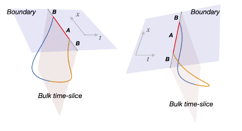
Figure 3: Here we present two different views of the same ‘extremal line’ for a subsystem in $d=2$, determined numerically. This plot has been generated for $T=1/2\pi$ and $\ell=1.12$, when the fluid is moving with a constant vlocity $v=0.5$. The two solution branches of (11), solved with the boundary conditions (12), have been separately represented by the yellow and the blue lines. The red line denotes the boundary subsystem $A$, while the gray line denotes a canonical time-slice on the boundary. It is noteworthy, that the extremal surface moves out of a constant time-slice in the bulk (denoted by the light-pink surface).

Numerical verification

We can adapt the procedure outlined in section 2.1 to d=2, and find a numerical solution to the equations for the extremal surface (8). In fig.3, we provide a representative plot of the extremal surface (which is a line for $d=2$). In our solutions we clearly observe that $t(\phi)$ has a non-trivial dependence on the world-volume coordinate $\phi$, implying that the extremal surface, even in the Schwarzschild coordinates (2), does not lie on the constant time-slice extended into the bulk.

With this extremal surface determined numerically, we can directly evaluate the regulated HEE for the boosted fluid (bf)

$$\Delta\mathcal{S}=\mathcal{S}^{{(\text{bf})}}-\mathcal{S}^{(\text{vac})}\equiv\frac{c}{6}~{}\Delta S_{E}$$ (26)

Here, the pre-factor $c/6=\mathcal{R}_{\text{AdS}}/4G_{N}$ has been introduced as a normalization which is convenient for presenting numerical results3. Our numerical results are exact in boost parameter $v$ and valid for arbitrary temperature. In fig.4, we numerically plot $\Delta S_{E}$ as a function of $v$ at fixed $\ell T$ and we find an excellent match with the analytical answer in (20). In particular, the divergence structure (25) is correctly reproduced by the numerics.

Figure 4: Plot of the regulated HEE (26) for the 1+1D boosted fluid (boosted BTZ) $\Delta S_{E}$ vs boost $v$. The fixed temperature for this plot is $T=1/2\pi$ and subsystem size is $\ell=2$. Note that since we have regulated our HEE with the vacuum HEE, the $v\rightarrow 0$ limit is non-zero and provides the regulated HEE for the static fluid at fixed temperature. The answer diverges as $v\rightarrow 1$ following (25).

2.2.2 Holographic Mutual information

Another useful measure of quantum entanglement for a given state is quantum mutual information. For non-overlapping subsystems $A$ and $B$, mutual information can be expressed in terms of entanglement entropy as follows

$$I(A,B)=S_{A}+S_{B}-S_{A\cup B},$$ (27)

where $S_{A}$ represents the entanglement entropy between the subsystem $A$ and its compliment. Given the property of strong subadditivity of entanglement entropy, this quantity is guaranteed to be positive ($I(A,B)\geq 0$). In addition, it is UV finite. With the help of (27) the holographic prescription for entanglement entropy can be adapted to compute quantum mutual information (see Nishioka:2009un ; Swingle:2010jz ; Fischler:2012uv ).

For the strip-shaped subsystems, let us consider both $A$ and $B$ to have the same size $\ell$, while the distance between the two is denoted by $x$. For the fluid flows with a constant velocity $v$, $I(A,B)$ depends on three dimensionless parameters. Apart from the fluid velocity $v$, the other two parameters are the ones which may be constituted with dimensionless ratios between $\ell$, $x$ and temperature $T$. Since, we have observed a peculiar diverging behaviour of entanglement entropy as the fluid velocity approaches its relativistic upper bound, we would now like to understand the behaviour of mutual information for large fluid velocities. For $d=2$, the existence of the analytical result (20) immediately implies an analytical formula for mutual information $I(A,B)=I(\ell,x,\beta,v)$, which is given by

$$I(\ell,x,\beta,v)=\frac{c}{6}\ln\left(\dfrac{\sinh^{2}\left(\frac{\pi\alpha(v)\ell}{\beta}\right)~{}\sinh^{2}\left(\frac{\pi\ell}{\alpha(v)\beta}\right)}{\sinh\left(\frac{\pi\alpha(v)x}{\beta}\right)~{}\sinh\left(\frac{\pi x}{\alpha(v)\beta}\right)~{}\sinh\left(\frac{\pi\alpha(v)(2\ell+x)}{\beta}\right)~{}\sinh\left(\frac{\pi(2\ell+x)}{\alpha(v)\beta}\right)}\right),$$ (28)

where $\alpha(v)$ is given in (19) and $\beta$ is the inverse temperature (3). When the subsystems $A$ and $B$ are very far away from each other $I(A,B)$ vanishes generically. In fact, $I(A,B)$ continuously reduces to zero at some finite critical distance ($x_{c}$) and remains zero for larger distances between $A$ and $B$. This fact is well understood in the holographic context Fischler:2012uv . The term $S_{A\cup B}$ in (27) has two extremal surfaces homologous to $A\cup B$. At the critical distance, dominance flips between these two extremal surfaces. This critical distance ($x_{c}$) depends on the properties of the underlying state, for example, it is determined by the temperature for a thermal state. In Fischler:2012uv , the functional dependence of this critical distance on temperature was computed for $v=0$. Given the exact result (28) in $d=2$, we can immediately generalize their result for a non-zero fluid velocity.

In fig.5(a), we have plotted $I(A,B)$ versus the fluid velocity $v$ at fixed $x/\ell$ and $T\ell$. We observe that, for a given separation $x$, there exists a critical velocity $v_{c}$ where mutual information vanishes. The value of $v_{c}$ increases as we decrease $x$, approaching its relativistic upper bound as $x\rightarrow 0$. Once the mutual information reaches zero, it remains so beyond $v_{c}$. At $v_{c}$, there is an exchange of dominance between the two extremal surfaces for $S_{A\cup B}$. This is exactly the same phenomenon which gives rise to a critical distance $x_{c}$ between $A$ and $B$, as we have described above. Here, we find that the deformation of the extremal surfaces, produced due to the fluid velocity (see fig.3), forces this exchange of dominance between the extremal surfaces, even when the two subsystems are close to each other ($x<x_{c}$). In fig.5(b) we demarcate the region in the $\{x/\ell,v\}$ plane, where mutual information is non-zero for a fixed temperature. As expected from the results of Fischler:2012uv , this region shrinks with the increase in temperature.

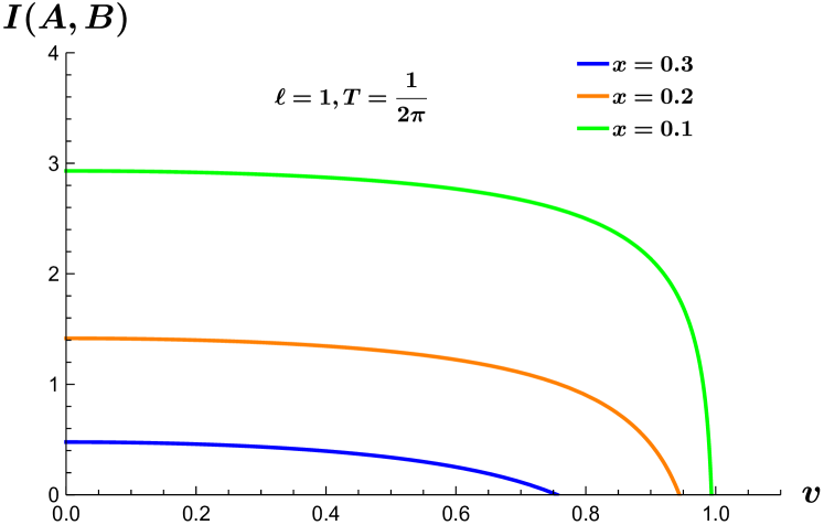
(a)

(b)

Figure 5: In (a) we plot the mutual information $I(A,B)$, using (28), as a function of the fluid velocity $v$, for fixed $x/\ell$ and $\ell T$. Note that there is a critical velocity $v_{c}$ where $I(A,B)$ vanishes for a given $x/\ell$. We have presented the plots corresponding to three different values of separation $x$. Clearly, $v_{c}$ increases with decrease in $x$. In (b), the shaded region below the bold lines, demarcates the values of $x/\ell$ and $v$ for which mutual information is non-zero. This region of non-zero $I(A,B)$ shrinks with the increase in temperature.

2.3 Higher dimensional fluids

In higher dimensions, we do not have any analytical results. But, it is straightforward to generalize the verified numerical procedure outlined for $d=2$ in section 2.2.1. The general procedure has already been outlined in section 2.1 for general dimensions. Therefore, skipping the details, we directly present the results of our numerical computations in this section.

The variation of the regulated HEE (26) versus the fluid velocity $v$, keeping $\ell T$ fixed, has been plotted in fig.6(a) for $d=3,4$. We observe that just like in $d=2$, the regulated HEE diverges as $v\rightarrow 1$. In fig.6(b), we demonstrate that the divergence occurs as $\Delta S_{E}\sim(1-v)^{-1/2}$ as $v\rightarrow 1$. Again, this behaviour is identical to that observed for $d=2$. With this observation, it is extremely tempting to conjecture that, in this set-up, the divergence in $\Delta S_{E}$ occurs due to a factor of $\gamma$. Perhaps this is universal across dimensions for a strip-shaped subsystems, with the fluid moving parallel to its short edge. It would be extremely interesting to understand the nature of this divergence for more general subsystem geometries.

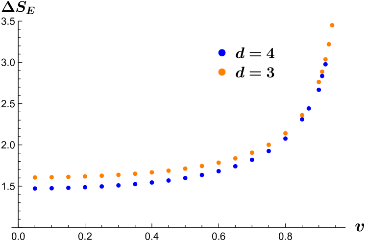
(a)

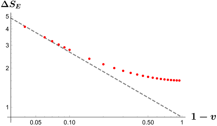
(b)

Figure 6: In (a) we plot the variation of regulated entanglement entropy $\Delta S_{E}$ as a function of the fluid velocity in $d=3,4$ for constant $\ell T=d/4\pi$. Note that $\Delta S_{E}$ diverges as $v\rightarrow 1$. In (b) we have displayed a log-log plot of $\Delta S_{E}$ versus $\epsilon_{v}=(1-v)$ in $d=3$, and for small values of $\epsilon_{v}$ we observe that the numerically computed values of $\Delta S_{E}$ tends towards the dashed straight line with slope $-1/2$. This demonstrates that $\Delta S_{E}$ scales as $(1-v)^{-1/2}$ as $v\rightarrow 1$.

Once we are able to compute the entanglement entropy with reliable numerics, it is straightforward to compute the mutual information (27) in higher dimensions. In fig.7, we plot the mutual information versus the fluid velocity in $d=3$. Even here, we notice a behaviour which is qualitatively identical to that in $d=2$ (see fig.5(a)). In particular, we observe that there is a critical velocity beyond which the mutual information vanishes. Again, this feature is also perhaps true across all dimensions.

Figure 7: Numerical plots exhibiting the variation of mutual information $I(A,B)$ with respect to fluid velocity $v$ in $d=3$.

3 Entanglement in hydrodynamic sound mode

3.1 Outline of the general procedure

After considering the steady state fluid configurations with a constant velocity, in this section, we proceed to analyse the entanglement structure of fluid states which are slightly out of equilibrium. More specifically, we shall focus on the propagating sound mode, which is ubiquitous in all systems admitting a macroscopic fluid description. Our set-up here, will again be holographic, which technically limits our observations to conformal relativistic fluids. However, our qualitative observations in this section would perhaps be more universal than the holographic context.

The sound mode is a fluctuating small amplitude perturbation over a stationary background. We will compute the HEE for the sound mode using the fluid-gravity correspondence Bhattacharyya:2007vjd . We shall now provide a brief overview of the general procedure adopted for this HEE computation.

The dual black brane solution providing a holographic description of the fluctuating states of a relativistic conformal fluid in $d=4$, with a controlled derivative expansion, was first provided in Bhattacharyya:2007vjd , which was subsequently generalized to other dimensions in VanRaamsdonk:2008fp ; Haack:2008cp ; Bhattacharyya:2008mz . Using these constructions, it is simple to read off the black brane geometries dual to the sound modes. Since these bulk geometries are constructed in the derivative expansion, they are valid when the wavelength ($\lambda=2\pi/k$) of the sound mode is large compared to the temperature scale ($\lambda T\gg 1$). Beside this small parameter $k/T$, the amplitude of the sound mode (say, $\epsilon$) also must be small, since it is a linearized solution to the fluid equations. We shall consider the amplitude ($\epsilon$) as the smallest of the two parameters.

Due to the linearized nature of the sound mode, the dual geometry of the fluctuating black brane has the following structure

$$ds^{2}_{d+1}=g_{ab}~{}dx^{a}dx^{b}=\left(g^{(0)}_{ab}+\epsilon~{}g^{(1)}_{ab}\right)dx^{a}dx^{b}$$ (29)

Here $g^{(1)}_{ab}$ is the $\epsilon$-order correction to the background metric $g^{(0)}_{ab}$, and we shall consider $g^{(0)}_{ab}$ to be the static black brane dual to the static fluid7. Since the background is static there is no $k$ dependence in $g^{(0)}_{ab}$, while $g^{(1)}_{ab}$ has a further expansion in powers of $k$ due to the derivative expansion corrections to the bulk metric.

Similar to the previous section, we would like to compute HEE for a strip-like subsystem over the fluid configuration with a propagating sound mode (see fig.1). The short-edge of the strip is of length $\ell$, and again, to keep the computations simple, we shall restrict ourselves to the scenario where the sound mode is propagating along the direction of the short edge. Apart from $k/T$ and $\epsilon$, the dimension $\ell$ of the subsystem introduces a third independent dimensionless parameter in the problem, which is given by $T\ell$. While there are no a priori restrictions on this parameter, in the holographic set-up, if we are to capture the thermal effects adequately, we must ensure that $T\ell\sim\mathcal{O}(1)$ or greater.

The HEE computation is accomplished by computing the area of the extremal surface as prescribed in (1) Hubeny:2007xt . Unlike the stationary scenario discussed in section 2, we now expect a non-trivial time dependence of HEE. If we parameterize our co-dimension 2 extremal surface ($\Gamma$) with the coordinates $\{\xi\}$, the induced metric on $\Gamma$ takes the form

$$\mathcal{G}_{\alpha\beta}=\frac{\partial x^{a}}{\partial\xi^{\alpha}}\frac{\partial x^{b}}{\partial\xi^{\beta}}g_{ab}$$ (30)

However, due to the decomposition (29), the induced metric also decomposes as

$$\mathcal{G}_{\alpha\beta}=\mathcal{G}^{(0)}_{\alpha\beta}+\epsilon~{}\mathcal{G}^{(1)}_{\alpha\beta},$$ (31)

where

$$\mathcal{G}^{(0)}_{\alpha\beta}=\frac{\partial x^{a}}{\partial\xi^{\alpha}}\frac{\partial x^{b}}{\xi^{\beta}}g^{(0)}_{ab},~{}~{}\mathcal{G}^{(1)}_{\alpha\beta}=\frac{\partial x^{a}}{\partial\xi^{\alpha}}\frac{\partial x^{b}}{\xi^{\beta}}g^{(1)}_{ab}.$$ (32)

The area of the co-dimension 2 surface $\Gamma$ is immediately given by the induced metric

$$A_{\Gamma}=\int\left(d\xi\right)^{d-1}\sqrt{\mathcal{G}}$$ (33)

where $\mathcal{G}$ is the determinant of the induced metric (30). However, due to (31) this area also has an expansion in amplitude

$$A_{\Gamma}=A^{(0)}_{\Gamma}+\epsilon~{}A^{(1)}_{\Gamma}$$ (34)

Here $A^{(0)}_{\Gamma}$ has the contribution from the background static geometry and constitutes the leading order piece in HEE. It is given by

$$A^{(0)}_{\Gamma}=\int(d\xi)^{d-1}\sqrt{\mathcal{G}^{(0)}}.$$ (35)

By the prescription (1), this area when evaluated over the extremal surface provides the entanglement of the strip subsystem for the fluid in static equilibrium. On the other hand the corrections due to the sound mode is captured by $A^{(1)}_{\Gamma}$, which is given by

$$A^{(1)}_{\Gamma}=\frac{1}{2}\int(d\xi)^{d-1}\sqrt{\mathcal{G}^{(0)}}~{}\mathcal{G}^{(1)}_{\alpha\beta}{\mathcal{G}^{(0)}}^{\alpha\beta}.$$ (36)

Note that, at first order in $\epsilon$, the functional in (36) is to be evaluated over the same surface $\Gamma$ that was obtained by extremizing $A^{(0)}$ in (35). The change in HEE produced due to the fluid sound mode is therefore given by

$$\Delta\mathcal{S}=\frac{A^{(1)}_{\Gamma}}{4G_{N}}$$ (37)

As in the previous section (see (14)), for our numerical plots, it will be convenient to work with the quantity $\Delta S_{E}=A^{(1)}_{\Gamma}/L^{(d-2)}$.

3.2 Sound mode in $d=2$

In $d=2$, conformal relativistic fluid dynamics is trivial and there are no non-trivial transport coefficients, in the uncharged sector. Therefore, the energy-momentum tensor is always of the perfect fluid form

$$T_{\mu\nu}=\mathcal{E}(T)u_{\mu}u_{\nu}+\mathcal{P}(T)P_{\mu\nu}.$$ (38)

The key difference of (38) with that of in higher dimensions (4), is that, (38) does not have any higher derivative corrections, even if the fluid variables ($T$ and $u^{\mu}$) have arbitrary space-time dependence. Here, the energy density $\mathcal{E}$ and pressure $\mathcal{P}$ must be equal (see (5)) so as to ensure tracelessness of the energy-momentum tensor - a requirement of conformality. All solutions to this system are non-dissipative. The two fluid variables - $T$ and the spatial component of normalized $u_{\mu}$ - are to be determined by the fluid equations which are given by the conservation of the energy-momentum tensor

$$\partial_{\mu}T^{\mu\nu}=0$$ (39)

Here, (39) gives us two independent equations, providing solutions for the two fluid variables. These solutions can have a non-trivial dependence on space-time coordinates, without requiring higher derivative corrections. Thus, unlike higher dimensions, the restrictions due to derivative expansion on the sound wave momentum $k$ (i.e. $k/T\ll 1$ ) does not apply for the $d=2$ fluid.

For any arbitrary solution of (39), an explicit holographic dual metric was constructed in Haack:2008cp

$$\begin{split}ds^{2}&=\frac{1}{z^{2}}\left(-\left(1-\frac{z^{2}}{\zeta^{2}}\right)u_{\mu}u_{\nu}dx^{\mu}dx^{\nu}+P_{\mu\nu}dx^{\mu}dx^{\nu}+2u_{\mu}dx^{\mu}dz\right)\\ &+\frac{2}{z}\partial_{\lambda}u^{\lambda}~{}u_{\mu}u_{\nu}dx^{\mu}dx^{\nu}-\frac{1}{z}u^{\lambda}\partial_{\lambda}\left(u_{\mu}u_{\nu}\right)dx^{\mu}dx^{\nu}\end{split}$$ (40)

The derivative corrections in the second line of (40) ensures that the metric is an exact solution to the Einstein equations, whenever the fluid parameters $u^{\mu}(x)$ and $T(x)=1/\left(2\pi\zeta(x)\right)$, as functions of the boundary coordinates $x^{\mu}$, solves (39). The explicit form of the fluid equations (39) is given by

$$u^{\mu}\partial_{\mu}\zeta=\zeta\partial_{\nu}u^{\nu},~{}~{}P_{\mu}^{~{}\nu}\partial_{\nu}\zeta=\zeta u^{\lambda}\partial_{\lambda}u_{\mu}.$$ (41)

The metric (40) is essentially diffeomorphic to the BTZ black hole Haack:2008cp , which on the gravity side, reflects the triviality of conformal hydrodynamics in $d=2$. The dynamics induced by these non-trivial diffeomorphisms serves as a toy model for hydrodynamics with a non-dissipative sound mode. Note that, (40) is similar to a fluid-gravity metric in higher dimensions (see (47), (59)) expanded upto first order in derivatives, but (40) is an exact solution. This absence of the requirement of a derivative expansion makes this setting particularly suitable to initiate a study of the HEE for the sound mode.

Linearized solutions

Let us denote the boundary coordinates with $x^{\mu}=\{t,x\}$ and express the two fluid functions in the following way

$$u^{\mu}=\gamma\{-1,v\},~{}~{}T=\frac{1}{2\pi\zeta},~{}~{}\text{where}~{}\gamma=\frac{1}{\sqrt{1-v^{2}}}$$ (42)

Then (41) admits the following linearized sound wave solution

$$\begin{split}\zeta&=\zeta_{0}\left(1+\epsilon\cos\left(\omega t-kx\right)+\mathcal{O}\left(\epsilon^{2}\right)\right)~{},~{}~{}\\ v&=\epsilon\cos\left(\omega t-kx\right)+\mathcal{O}\left(\epsilon^{2}\right),~{}~{}\text{with}~{}\omega=k,\end{split}$$ (43)

where $\zeta_{0}$ determines the background temperature.

Exploiting linearization, it is straightforward to superimpose these sinusoidal solutions with a Gaussian weight to constitute a propagating wave-packet solution of the form

$$\begin{split}\zeta&=\zeta_{0}\left[1-\epsilon~{}\exp\left(-\frac{\left(x-t\right)^{2}}{2\sigma^{2}}\right)+\mathcal{O}\left(\epsilon^{2}\right)\right]~{},~{}~{}\\ v&=\epsilon~{}\exp\left(-\frac{\left(x-t\right)^{2}}{2\sigma^{2}}\right)+\mathcal{O}\left(\epsilon^{2}\right),\end{split}$$ (44)

where $\sigma$ is the width of the pulse. Clearly, (44) is also a linearized solution of the fluid equations (41). Note that, physically this solution corresponds to a energy density or pressure pulse propagating in the positive $x$-direction. The amplitude of this pulse is proportional to $\epsilon$, which in general, denotes a small positive or negative correction to their background values. In our subsequent numerical computations, we shall consider $\epsilon$ in (44) to be positive, corresponding to a positive correction to the background energy density.

We can plug in the solutions (43) and (44) into (40) to obtain the corresponding bulk metric, which will be clearly of the form (29). We can then use the procedure outlined in section 3.1 to compute corrections to HEE corresponding to these fluid solutions.

Extremal surface in the background

In order to implement the algorithm of section 3.1, we need to find the extremal surface in the background metric (see (29))

$$g_{ab}^{(0)}dx^{a}dx^{b}=\frac{1}{z^{2}}\left(-\left(1-\frac{z^{2}}{\zeta_{0}^{2}}\right)dt^{2}-2dtdz+dx^{2}\right)$$ (45)

This is simply the static BTZ black brane written in Eddington-Finkelstein (EF) coordinates and is obtained by plugging in the $\mathcal{O}(\epsilon^{0})$ terms of (43) and (44) into (40).

If we now consider a boundary subsystem ($A$) of length $\ell$ centered at the origin ($x\in[-\ell/2,\ell/2]$). Here, the extremal surface in EF coordinates anchored on and homologous to $A$ can be written down analytically. It is simply a coordinate transformation (see appendix A) of the corresponding extremal surface in Schwarzschild coordinates Bhattacharya:2013bna . The explicit form of the embedding equations for this extremal surface in EF coordinates is given by

$$\begin{split}&z(\phi)=z_{\star}~{}\cos\phi\\ &x(\phi)=\zeta_{0}~{}\ln\left(\dfrac{\kappa\sin\phi+\sqrt{1-\kappa^{2}\cos^{2}\phi}}{\sqrt{1-\kappa^{2}}}\right)\\ &t(\phi)=t_{b}-\text{arctanh}\left(\kappa\cos\phi\right)\\ &\text{where}~{}z_{\star}=\zeta_{0}~{}\kappa,~{}\text{and}~{}\kappa=\tanh\left(\frac{\ell}{2\zeta_{0}}\right).\end{split}$$ (46)

Here $t_{b}$ denotes the boundary canonical time-slice which contains the subsystem $\mathcal{A}$. The dependence of HEE on $t_{b}$ provides its time evolution.

Numerical results for HEE

In order to find $\Delta S_{E}$, we must evaluate the functional (36) over the extremal surface (46). The metric correction $g^{(1)}_{ab}$ in (29), and hence the corrections to the induced metric $\mathcal{G}^{(1)}_{\alpha\beta}$ is obtained by computing the $\mathcal{O}(\epsilon)$ term from (40) after substituting the linearized solutions (43) and (44) . We will now present our results for $\Delta S_{E}$ in terms of numerical plots.

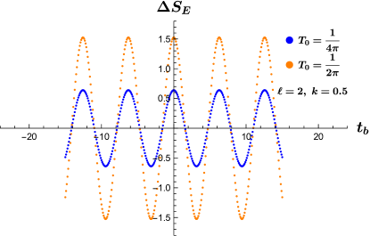
Figure 8: $\Delta S_{E}$ vs $t_{b}$ for sound wave in $d=2$.

Sound-waves:

We now compute $\Delta S_{E}$ for the scenario where a non-dissipative sound-wave (43) with momentum $k$ constantly passes over our subsystem $A$. Once we assume a small value of the parameter $\epsilon$, there are two more independent dimensionless parameters in the problem - $\ell T_{0}$ , $k/T_{0}$, $T_{0}$ being the background temperature.

The variation of $\Delta S_{E}$ with boundary-time ($t_{b}$) has been shown in fig.8. We find a periodic variation of HEE, which was expected due to the sinusoidal nature of the fluid configuration. The period of the oscillations are given by $2\pi/k$ and is independent of temperature. This was expected from the fact that the time-dependence only arises through the term $\cos kt$ appearing in (43). In the embedding equations (46), $t$ goes linearly with $t_{b}$, which gives rise to a term proportional to $\cos kt_{b}$ in final linearized answer.

The amplitude of these oscillations is determined both by the temperature and $k$, for a fixed $\ell$. From fig.8 we see that for fixed $k$, this amplitude increases with increase in temperature. Recall that there exists no restriction on the value of $k$ here, due to the lack of any derivative expansion for the $d=2$ conformal fluid. So, we can plot this amplitude for arbitrary $k$ at a fixed temperature.

(a)

(b)

Figure 9: In (a) we plot the variation of $\Delta S_{E}$ at $t_{b}=0$ as a function of $k\ell$ for sound mode in $d=2$. This explicates the dependence of the amplitude of $\Delta S_{E}$ on $k$. We find an interesting quasi-periodic behaviour of $\Delta S_{E}$ with respect to $k$. In (b) we show that the distance between the first two zeros of $\Delta S_{E}(t_{b}=0)$ in (a), decreases with increase in temperature.

In fig.9(a), we study the variation of $\Delta S_{E}$ with respect to $k$ on a fixed boundary-time slice $t_{b}=0$. It is very interesting to note that for large values of $k$, $\Delta S_{E}$ behave sinusoidally with $k$. In particular, there exists special values of $k$ for which $\Delta S_{E}$ vanishes. The distance $\Omega$ between the first two zeros of $\Delta S_{E}(t_{b}=0)$, in fig.9(a), as well as the period of oscillation for large $k\ell$, is determined by the temperature. In fig.9(b), we have shown that the value of $\Omega$ decreases with the increase in temperature.

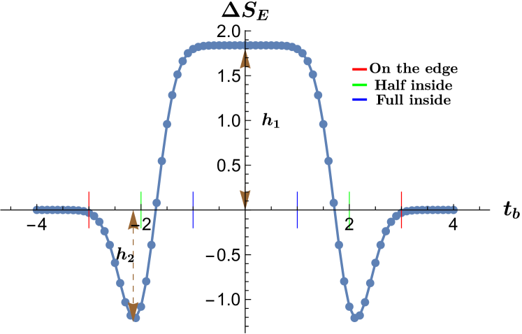
(a)

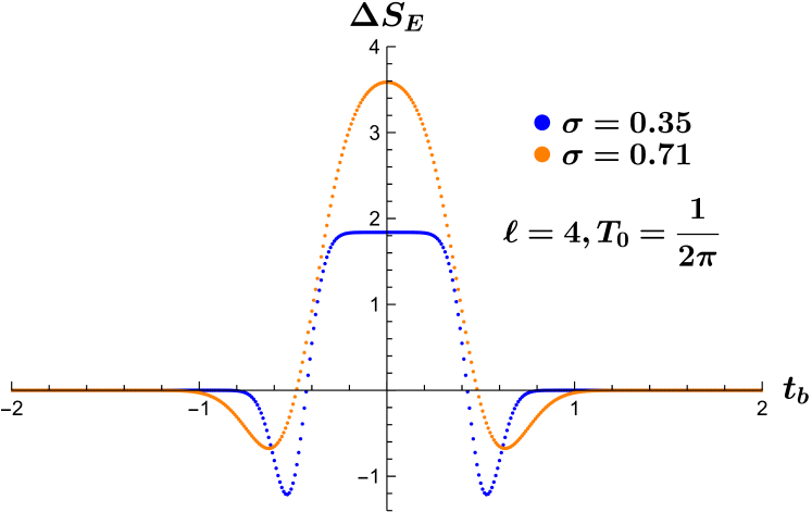
(b)

Figure 10: In (a) we plot the variation of $\Delta S_{E}$ with respect to boundary time $t_{b}$, as a pressure or energy density pulse travels across the subsystem $A$. We have chosen the pulse width $\sigma=0.35$, while the size of the subsystem has been taken to be $\ell=4$. The background temperature is kept at $T_{0}=1/2\pi$. At time $t_{b}=\mp 3$ (shown with the red line), the edge of the pulse touches the subsystem as it starts entering it (or completely leaves it). At time $t_{b}=\mp 2$, half of the pulse has entered (left) the subsystem, which appears to be close to the maximum value of the dip. Finally, at $t_{b}=\mp 1$ the pulse has completely entered the subsystem (or about to leave it). Note that, for time-interval ($t_{b}=-1$ to $t_{b}=+1$) during which the pulse lives inside the subsystem, $\Delta S_{E}$ saturates to a constant value. In (b) we demonstrate how the time evolution of $\Delta S_{E}$ varies as we change the width of the pulse.

Propagating pulse:

We now consider a traveling wave-packet - a pressure or energy density pulse (44). We record the change in HEE as this pulse traverses the subsystem $A$. As expected, when the pulse is completely outside the subsystem $A$, travelling towards or away from it, $\Delta S_{E}$ is zero. But, while the pulse moves across the subsystem, $\Delta S_{E}$ exhibits an interesting time dependence, as shown in fig.10.

After fixing $\epsilon$ to a small value, there are three length scales in this problem as well. Apart from $\ell$ and $T$, there is $\sigma$ which is the width of the pulse. When the pulse of positive energy density moves completely inside the subsystem $A$, it perhaps drags in some ‘matter’ within $A$ from outside. From this naive picture we can expect that there will be an increase in $\Delta S_{E}$, which would eventually go down to zero, when the pulse passes out. In fig.10(a) we see that this expectation is almost correct, except that there is a additional feature. When the pulse enters (or exits) the subsystem, we find that there is an interesting dip in $\Delta S_{E}$ before the expected rise (or fall).

In fig.10(b), we demonstrate that if the width of the pulse $\sigma$ is comparable to or larger than the size of the subsystem $\ell$, there is a unique peak of $\Delta S_{E}$, which corresponds to the time when the maxima of the peak coincides with the central point of the subsystem. On the other hand, when $\sigma$ is significantly smaller than $\ell$, the $\Delta S_{E}$ saturates to a constant value for the duration the pulse spends inside the subsystem. In both the case, the dip in $\Delta S_{E}$, during entry or exit, persists.

The extent of the dip ($h_{2}$), and the maximum value of $\Delta S_{E}$ during the process ($h_{1}$), both are determined by the background temperature $T_{0}$, for a fixed width of the pulse. In fig.11, we plot the variation of $h_{1}$ and $h_{2}$ with respect to background temperature. We note that $h_{2}$ decreases with temperature, while $h_{1}$ increases. It appears from fig.11(b) that $h_{2}$ would perhaps tend to a finite value as $T_{0}\rightarrow 0$. This suggests that the physical origin of this dip may be due to some non-thermal effect, which comes into play when propagating fluctuations of energy-momentum tensor tries to enter or exit the subsystem.

(a)

(b)

Figure 11: The variation of the height $h_{1}$ and dip $h_{2}$ of $\Delta S_{E}$ (in fig.10) as a function of temperature.

3.3 Dissipative sound mode in higher dimensions

We now move on to higher dimension, where the sound mode is dissipative. Unlike, $d=2$, in higher dimensions we have a derivative expansion, whose validity restricts our analysis only to long wavelengths i.e. $k/T\ll 1$. The HEE for these dissipative states are studied for a subsystem of length $\ell$, so that $T\ell\sim\mathcal{O}(1)$. Here, we will follow the general procedure outlined in section 3.1, which will closely resemble the analysis in section 3.2.

We will first perform our analysis for $d=3$, where the time-dependence of HEE is predictably decaying sinusoidal, following the form of the sound mode, but we find an interesting phase difference between them, which carries non-trivial information regarding the entanglement structure of the state. We then move on to $d=4$, where apart from this phase, we observe a subleading UV divergence in HEE for the sound mode. Such an additional UV divergence, was absent in $d=2,3$. Since, our analysis is partially numerical, we therefore, restrict our analysis only up to $d=4$, but the qualitative features of the phase shift and the additional UV divergence is expected to be straightforwardly extended to higher dimensions.

3.3.1 $d=3$

Our starting point of this analysis is the holographic dual to $2+1$D boundary relativistic fluid, which is given by the $3+1$D bulk metric VanRaamsdonk:2008fp ; Haack:2008cp ; Bhattacharyya:2008mz

$$\begin{split}ds^{2}&=\frac{2}{z^{2}}u_{\mu}dx^{\mu}dz-\frac{1}{z^{2}}f^{(3)}(z)u_{\mu}u_{\nu}dx^{\mu}dx^{\nu}+\frac{1}{z^{2}}P_{\mu\nu}dx^{\mu}dx^{\nu}\\ &+\mathfrak{a}\frac{2\,\zeta}{z^{2}}\,F^{(3)}(z)\sigma_{\mu\nu}dx^{\mu}dx^{\nu}+\mathfrak{b}\frac{1}{z}u_{\mu}u_{\nu}(\partial_{\lambda}u^{\lambda})dx^{\mu}dx^{\nu}-\frac{1}{z}u^{\lambda}\partial_{\lambda}(u_{\nu}u_{\mu})dx^{\mu}dx^{\nu}+{\cal O}(\partial)^{2}\end{split}$$ (47)

where, the projector $P_{\mu\nu}$ has the usual definition, and

$$\begin{split}&\sigma^{\mu\nu}=\frac{1}{2}P^{\mu\alpha}P^{\nu\beta}(\partial_{\alpha}u_{\beta}+\partial_{\beta}u_{\alpha})-\frac{1}{2}(\partial_{\alpha}u^{\alpha})P^{\mu\nu}\\ &f^{(3)}(z)=1-\frac{z^{3}}{\zeta^{3}},\quad F^{(3)}(z)=\frac{1}{6}\left[\sqrt{3}\,\pi-2\sqrt{3}\,\tan^{-1}\frac{2\,\zeta+z}{\sqrt{3}\,z}+3\log\frac{\zeta^{2}+\zeta\,z+z^{2}}{\zeta^{2}}\right]\end{split}$$

Also, compared to the original metric reported in VanRaamsdonk:2008fp ; Haack:2008cp ; Bhattacharyya:2008mz , we have introduced two additional parameters which must be set to $\mathfrak{a}=1,\mathfrak{b}=1$ so as to ensure that (47) is a solution to Einstein’s equations. The terms, whose coefficients are $\mathfrak{a}$ and $\mathfrak{b}$, will play an important role in our discussion, which is why we have chosen to track them through the calculations with the help of these two parameters. We shall report all our results setting $\mathfrak{a}=1,\mathfrak{b}=1$, and refer to them only when necessary for contextual clarity.

As usual, we denote the boundary coordinates with $x^{\mu}=\{t,x,y\}$, while the temperature $T$ (3) and velocity $u_{\mu}=\gamma\{-1,v,0\}$ constitutes the fluid variables. The metric (47) is a solution of Einstein’s equation provided the fluid variables satisfy $\partial_{\mu}T^{\mu\nu}=0$ where, in this case, the constitutive relation reads

$$T_{\mu\nu}=\mathcal{P}\left(\eta_{\mu\nu}+3\,u_{\mu}u_{\nu}\right)-2\,\eta\,\sigma_{\mu\nu}+{\cal O}(\partial)^{2}.$$ (48)

where the pressure density $\mathcal{P}=(4\pi T/3)^{3}$ and shear viscosity $\eta=(4\pi T/3)^{2}$.

Linearized sound-wave solutions

Here, the fluid equations admit the following linearized sound wave solution

$$\begin{split}\zeta&=\zeta_{0}\left(1+\epsilon\ \exp[-i(\omega\,t-k\,x)]+~{}\mathcal{O}(\epsilon^{2})\right)\\ v&=\epsilon\,v_{1}\exp[-i(\omega\,t-k\,x)]+~{}\mathcal{O}(\epsilon^{2})\end{split}$$ (49)

with,

$$\omega=\pm\frac{1}{\sqrt{2}}k-\frac{i\zeta_{0}}{6}k^{2}+{\cal O}(k^{3}),~{}~{}v_{1}=\sqrt{2}+i\frac{\zeta_{0}k}{3}+\mathcal{O}(k^{2})$$

Note that due to the imaginary piece in the dispersion relation, the fluctuations are damped exponentially by a factor of $\exp(-\lambda t)$, where the damping constant $\lambda=\frac{1}{6}\eta k^{2}\zeta_{0}^{3}$ is determined by shear viscosity.

Extremal surface in the background

To implement the general procedure of calculating $\Delta S$ (see section 3.1), we have to calculate the extremal surface in the static background metric

$$ds^{2}=\frac{1}{z^{2}}\left[-2\,dt\,dz-\left(1-\frac{z^{3}}{\zeta_{0}^{3}}\right)dt^{2}+dx^{2}+dy^{2}\right]\,,$$ (50)

This metric is in Eddington-Finklestein. Therefore, following (77), we can choose the ansatz for the extremal surface to be

$$\Gamma:~{}x=x(z),~{}t=t_{b}-h(z),~{}z=z,~{}y=\tilde{y},$$ (51)

where,

$$h(z)=\int_{0}^{z}\frac{dz^{\prime}}{\left(1-\frac{z^{\prime 3}}{\zeta_{0}^{3}}\right)}=\frac{\zeta_{0}}{6}\left(2\sqrt{3}\,\tan^{-1}\frac{2\,z+\zeta_{0}}{\sqrt{3}\,\zeta_{0}}+\log\frac{z^{2}+z\,\zeta_{0}+\zeta_{0}^{2}}{(\zeta_{0}-z)^{2}}-\frac{\pi}{\sqrt{3}}\right)$$ (52)

The ansatz leads to the following expression for $A_{\Gamma}^{(0)}$ (see (35))

$$A_{\Gamma}^{(0)}=\int\sqrt{\mathcal{G}_{0}}\,dz\,dy=2\,L\int_{0}^{z_{\star}}\frac{dz}{z^{2}}\left[\frac{1}{1-\frac{z^{3}}{\zeta_{0}^{3}}}+x^{\prime}(z)^{2}\right]^{\frac{1}{2}}$$ (53)

which upon extremization yields

$$x^{\prime}(z)=\frac{\frac{z^{2}}{{z_{\star}}^{2}}}{\sqrt{1-\frac{z^{3}}{\zeta_{0}^{3}}}\sqrt{1-\frac{z^{4}}{{z_{\star}}^{4}}}}$$ (54)

Again, $z_{\star}$ is the turning point, which is determined in terms of the boundary subsystem length $\ell$. The integration in (54) is performed numerically.

Computation of $\Delta S_{E}$ for sound mode

The change in the area of the extremal surface $\Gamma$ in (51) due to linearized sound wave fluctuations, which captures the corresponding change in entanglement entropy, is given by (see (36))

$$\Delta S_{E}=\frac{A_{\Gamma}^{(1)}}{L}=\int_{0}^{z_{\star}}dz\,\sqrt{{\mathcal{G}_{0}}}\,{\mathcal{G}}_{0}^{\alpha\beta}{\mathcal{G}}^{1}_{\alpha\beta}=\int_{0}^{z_{\star}}dz\,\mathfrak{I}(z)$$ (55)

where, $\mathfrak{I}(z)$ has the following form

$$\mathfrak{I}(z)=e^{-\lambda\,t(z)}\exp\left({i\,k\left(\frac{t(z)}{\sqrt{2}}+x(z)\right)}\right)\left(\mathfrak{I}_{R}(z)+i\,\mathfrak{I}_{I}(z)\right)$$ (56)

where,

$$\begin{split}\mathfrak{I}_{I}&=k\left(-(\mathfrak{a}-\mathfrak{b})\frac{\sqrt{2}}{z}+\frac{2\,\zeta_{0}}{3\,{z_{\star}}^{2}}+{\cal O}(z)\right)+{\cal O}(k^{2})\\ \mathfrak{I}_{R}&=\left(\frac{2\sqrt{2}}{{z_{\star}}^{2}}+{\cal O}(z)\right)+{\cal O}(k^{2})\end{split}$$ (57)

We have expanded $\mathfrak{I}_{I}$ and $\mathfrak{I}_{R}$ in $z$, about the asymptotic boundary, to demonstrate the following interesting feature of the integrand $\mathfrak{I}(z)$.

Let us recall that since $\Delta S_{E}$ captures the change in HEE compared to the thermal background value, we do not expect any leading order divergence in $\Delta S_{E}$, but there may be subleading divergences. Also, since we are in d=3, a subleading divergence would mean a logarithmic divergence. Clearly, in (57) we see that there is a term in $\mathfrak{I}_{I}$ which is $\mathcal{O}\left(1/z\right)$. This term may lead to a potential UV logarithmic divergence upon performing the integration in (55). However, the term is proportional to $(\mathfrak{a}-\mathfrak{b})$ and we know for the fluid metric to satisfy the Einstein’s equation we must have $\mathfrak{a}=1$ and $\mathfrak{b}=1$. Thus consistency with the right fluid-gravity metric necessitates the vanishing of this potentially divergent term. We should note that this cancellation occurs only at the linear order in $k$. This is the order up to which our calculation is reliable since we have considered only first order in derivative expansion. It is possible that at higher order this subleading logarithmic divergence exists with some universal coefficient. As we shall see below, this magical cancellation does not happen in $d=4$, where a subleading UV divergence is observed.

(a)

(b)

Figure 12: In (a) we plot the variation of $\Delta S_{E}$ with time $t_{b}$ for the sound mode in $d=3$. This variation is trivially damped harmonic as predicted by (58). In (b) we plot the phase of the amplitude $\Phi_{\mathfrak{S}}$ as a function of background temperature $T_{0}$.

From the structure of (56) and the embedding equation (51), it is immediately clear that $\Delta S_{E}$ has a straightforward dependence on $t_{b}$, which factors out of the integral. In fact upon performing the integration in (55), we should have the following schematic form

$$\begin{split}\Delta S_{E}(t_{b})&=e^{-\lambda\,t_{b}}\exp\left({i\,k\frac{t_{b}}{\sqrt{2}}}\right)\mathfrak{S}(k,\ell,T),\\ \text{where},~{}~{}\mathfrak{S}(k,\ell,T)&=\mathfrak{S}^{(0)}(\ell,T)+k~{}\mathfrak{S}^{(1)}(\ell,T)+\mathcal{O}(k^{2}).\end{split}$$ (58)

The real and imaginary parts of $\Delta S_{E}(t_{b})$ has been plotted in fig.12(a), which is clearly damped harmonic due to form (58). The phase of $\mathfrak{S}$, which we denote by $\Phi_{\mathfrak{S}}$, represent a phase shift in $\Delta S_{E}$ compared to the original sound wave perturbations (49). The variation of this phase with respect the $T\ell$, for a fixed $k$, has been shown in fig.12(b). We find that this phase has a weak dependence on temperature, and exhibits a growing trend towards high temperature.

3.3.2 $d=4$

The calculation in $d=4$ proceeds in parallel with that in $d=3$. We consider the following fluid-gravity metric Bhattacharyya:2007vjd , corrected up to first order in derivative expansion in $4+1$ bulk dimension

$$\begin{split}ds^{2}&=\frac{2}{z^{2}}u_{\mu}dx^{\mu}dz-\frac{1}{z^{2}}f(z)u_{\mu}u_{\nu}dx^{\mu}dx^{\nu}+\frac{1}{z^{2}}P_{\mu\nu}dx^{\mu}dx^{\nu}\\ &+\mathfrak{a}\frac{2\,\zeta}{z^{2}}\,F(z)\sigma_{\mu\nu}dx^{\mu}dx^{\nu}+\mathfrak{b}\frac{2}{3\,z}u_{\mu}u_{\nu}(\partial_{\lambda}u^{\lambda})dx^{\mu}dx^{\nu}-\frac{1}{z}u^{\lambda}\partial_{\lambda}(u_{\nu}u_{\mu})dx^{\mu}dx^{\nu}+{\cal O}(\partial)^{2}\end{split}$$ (59)

where,

$$\begin{split}f(z)=1-\frac{z^{4}}{\zeta^{4}},~{}\text{and}~{}F(z)=\frac{1}{4}\left(\log\frac{(z+\zeta)^{2}(z^{2}+\zeta^{2})}{\zeta^{4}}-2\tan^{-1}\frac{\zeta}{z}+\pi\right)\end{split}$$ (60)

Just like in $d=3$, we have introduced two constant parameters $\mathfrak{a}$ and $\mathfrak{b}$ in the metric, which must take the values $\mathfrak{a}=1$ and $\mathfrak{b}=1$, so as to ensure (59) solves Einstein’s equation.

We denote the boundary coordinates with $x^{\mu}=\{t,x,y_{1},y_{2}\}$ and express the two fluid variables as

$$u_{\mu}=\gamma\{-1,v,0,0\},\quad T=\frac{1}{\pi\,\zeta}.$$ (61)

The fluid variables in (59) must satisfy the constraint equation

$$\partial_{\mu}T^{\mu\nu}=0.$$ (62)

where,

$$T_{\mu\nu}=\frac{1}{\zeta^{4}}\left(\eta_{\mu\nu}+4\,u_{\mu}u_{\nu}\right)-\frac{2}{\zeta^{3}}\sigma_{\mu\nu}+{\cal O}(\partial)^{2}$$ (63)

We consider the linearized sound wave solution

$$\begin{split}\zeta&=\zeta_{0}\left(1+\epsilon\ \exp[-i(\omega\,t-k\,x)]+~{}\mathcal{O}(\epsilon^{2})\right)\\ v&=\epsilon\,v_{1}\exp[-i(\omega\,t-k\,x)]+~{}\mathcal{O}(\epsilon^{2})\\ \text{with},~{}~{}\omega&=\pm\frac{1}{\sqrt{3}}k-\frac{i\zeta_{0}}{6}~{}k^{2}+{\mathcal{O}}(k)^{3},~{}v_{1}=\sqrt{3}+i\frac{k\zeta_{0}}{2}+{\mathcal{O}}(k)^{2}.\end{split}$$ (64)

Note that, in $d=4$ the damping constant $\lambda=\frac{1}{6}\eta k^{2}\zeta_{0}^{4}$. As in $d=3$, the required surface is to be extremized in the background geometry

$$ds^{2}=\frac{1}{z^{2}}\left(-2\,dt\,dz-\left(1-\frac{z^{4}}{\zeta_{0}^{4}}\right)dt^{2}+dx^{2}+dy_{1}^{2}+dy_{2}^{2}\right)\,.$$ (65)

The ansatz for the extremal surface in Eddington-Finkelstein coordinates is again

$$\Gamma:~{}x=x(z),~{}t=t_{b}-h(z),~{}z=z,~{}y_{i}=\tilde{y}_{i},$$ (66)

where

$$h(z)=\int_{0}^{z}\frac{dz^{\prime}}{\left(1-\frac{z^{\prime 4}}{\zeta_{0}^{4}}\right)}=\frac{\zeta_{0}}{2}\tan^{-1}\frac{z}{\zeta_{0}}-\frac{\zeta_{0}}{4}\log[\zeta_{0}-z]+\frac{\zeta_{0}}{4}\log[\zeta_{0}+z].$$ (67)

and

$$x^{\prime}(z)=\frac{\frac{z^{3}}{{z_{\star}}^{3}}}{\sqrt{1-\frac{z^{4}}{\zeta_{0}^{4}}}\sqrt{1-\frac{z^{6}}{{z_{\star}}^{6}}}},$$ (68)

which is numerically integrated to obtain the necessary minimal surface. With the help of this extremal surface, the change in HEE due to the sound mode (64) is evaluated

$$\Delta S_{E}=\frac{A_{\Gamma}}{L^{2}}=\int^{z_{\star}}_{0}dz~{}\mathfrak{I}(z),$$ (69)

where, $\mathfrak{I}(z)$ has the following schematic form

$$\mathfrak{I}(z)=e^{-\lambda t(z)}\exp\left[{i\,k\left(\frac{t(z)}{\sqrt{3}}+x(z)\right)}\right]\left(\mathfrak{I}_{R}(z)+i\,\mathfrak{I}_{I}(z)\right)$$ (70)

where, near the asymptotic boundary ($z\rightarrow 0$), we have

$$\begin{split}\mathfrak{I}_{I}&=k\left(-(2\mathfrak{a}-\mathfrak{b})\frac{2}{\sqrt{3}z^{2}}+\frac{\zeta_{0}}{{z_{\star}}^{3}}+{\mathcal{O}}(z)\right)+{\cal O}(k^{2})\\ \mathfrak{I}_{R}&=\left(\frac{2\sqrt{3}}{{z_{\star}}^{3}}+{\cal O}(z)\right)+{\cal O}(k^{2})\end{split}$$ (71)

Recalling that $\mathfrak{a}=1,\mathfrak{b}=1$, we conclude that there exists a $\mathcal{O}(1/z^{2})$ term in the integrand $\mathfrak{I}(z)$. Once integrated, this term will give rise to a term in $\Delta S_{E}$ which is proportional to $1/\epsilon_{{\text{uv}}}$, where $\epsilon_{{\text{uv}}}\rightarrow 0$ is the UV cut-off. Note that this divergence is subdominant compared to the ‘area law’ divergence Nishioka:2009un , which for $d=4$ is proportional to $1/\epsilon_{{\text{uv}}}^{2}$ . We should emphasize that our observation is limited to $\mathcal{O}(k)$, and it is possible that there are other subleading divergences at higher order in the derivative expansion.

The integral in $\Delta S_{E}$ can be performed numerically only after extracting out the divergence. The integrated answer has the final schematic form

$$\begin{split}\Delta S_{E}(t_{b})&=e^{-\lambda\,t_{b}}\exp\left({i\,k\frac{t_{b}}{\sqrt{3}}}\right)\left(-\frac{2k}{\sqrt{3}\epsilon_{{\text{uv}}}}+\mathfrak{S}(k,\ell,T)\right),\\ \text{where},~{}~{}\mathfrak{S}(k,\ell,T)&=\mathfrak{S}^{(0)}(\ell,T)+k~{}\mathfrak{S}^{(1)}(\ell,T)+\mathcal{O}(k^{2}).\end{split}$$ (72)

Here, the function $\mathfrak{S}(k,\ell,T)$ is UV finite and has the same qualitative form as in $d=3$ (see fig.12). Also, recall that we have rescaled HEE by a factor of $L^{2}$. Hence, this UV divergent piece in the full HEE is proportional to $(kL^{2}/\epsilon_{{\text{uv}}})e^{-\lambda\,t_{b}}\exp\left({i\,k\frac{t_{b}}{\sqrt{3}}}\right)$, which is subdominant compared to the area law divergence proportional to $L^{2}/\epsilon_{{\text{uv}}}^{2}$. Clearly, the subleading divergence decays with time and disappears in the final equilibrium state.

4 Discussions

In this paper, we have studied holographic entanglement entropy for two varieties of fluid configurations. At first, we have considered a stationary configuration where the fluid moves with a constant velocity. Here we find that HEE generically increases with an increase in fluid velocity when the other parameters are held fixed. Also, as the fluid approaches its relativistic upper bound $v\rightarrow 1$, the regulated HEE diverges. From our analysis, it appears that this divergence is proportional to a factor of $\gamma$ in $d=2,3$. This is perhaps a universal behaviour for strip-shaped subsystems which we consider here. Admittedly, we do not have a clear understanding of this additional divergence. However, we would like to point out that a similar divergence was also present in the earlier perturbative results of Blanco:2013joa , although the structure of the divergence is slightly different in our non-perturbative treatment.

In this context, we also study holographic mutual information between two non-overlapping subsystems of the same size, separated by a distance $x$. When the fluid velocity is zero ($v=0$), it is known from previous work Fischler:2012uv that this mutual information vanishes at large $x$, while it is non-zero at small $x$. There is a ‘phase-transition’-like effect for mutual information at some critical distance $x_{c}$. For our steady state fluid flows, we find that even when the subsystems are close by ($x<x_{c}$), there exists a critical value of fluid velocity $v_{c}$ above which mutual information vanishes and remains zero for higher velocities. This occurs due to the flip of dominance between extremal surfaces, similar to what is observed when at $v=0$, the separation between the subsystems is increased. This critical velocity exists for all values of $x<x_{c}$. We find that $v_{c}$ increases with a decrease in the separation between the two subsystems, and $v_{c}\rightarrow 1$ as the separation approaches zero. This result follows from an analytical formula in $d=2$ (see (28)), while it has been verified numerically in $d=3$ (see fig.7). Again, we think, the qualitative aspects of this observation straightforwardly generalize to higher dimensions.

Our computation of entanglement measures for the steady-state fluid flow has a few immediate generalizations. In our work, we have always assumed that the fluid velocity is along the short edge of the strip. This may be generalized to a general angle, giving rise to a richer structure of HEE. It is tempting to speculate that, as we vary this angle, there may be a phase-transition-like effect as observed in Narayan:2012ks . Also, along this direction, generalizing our work to other shapes for the subsystem should also be interesting.

We then proceed to study HEE for the sound mode excitation of the fluid. Firstly, in $d=2$ the sound mode is non-dissipative. The variation of HEE with respect to boundary time is, in a way trivial since it has a predictable sinusoidal behaviour mimicking that of the fluid variables in the linearized approximation. However, it is observed that the amplitude of HEE has a very interesting dependence on the momentum $k$ of the sound waves. This behaviour is quasi-periodic, with HEE vanishing at specific values of $k$, which are determined by the background temperature (see fig.9(a)). The sound modes may be superimposed to form a traveling Gaussian wave-packet, which is a positive pressure or energy density pulse. While this pulse moves across the subsystem of interest, HEE generically experiences a jump. However, we find that when the pulse enters or exits the subsystem, there is a curious dip in HEE (see fig.10). The pulse may also be thought of as a ‘semi-local’ quench with the energy-momentum tensor, and similar effects on HEE may also be visible for a non-thermal background as well. It would be very interesting to investigate the physical origin of this dip in future work.

Finally, we have considered the sound mode in $d=3,4$, where it is dissipative. The fluid fluctuations are damped due to the shear viscosity, and at late times these configurations settle down to equilibrium. Due to our linearized approximation, the time dependence of HEE follows this damped oscillatory behaviour of the fluid variables (see fig.12). But, the amplitude of these oscillations is significantly interesting due to a phase which is physically relevant. The most noteworthy feature in this calculation is the presence of an additional UV divergence in $d=4$, which is subleading compared to the ‘area law divergence’. This divergence is dynamical in the sense that its coefficient is exponentially damped at late times and therefore disappears in the final equilibrium state. In $d=3$, potentially, there was the possibility of such a subleading logarithmic divergence, but it is absent due to a miraculous cancellation at first order in derivative expansion. The possibility of the existence of this divergence in $d=3$ when higher order derivatives are taken into account remains open. The physical origin of this divergence in $d=4$ is not very clear. Dissipation is clearly not the reason, as it is absent for the $d=3$ sound mode. It is possible that this is some artifact of the derivative expansion. In future investigations, it would definitely be very interesting to develop a better understanding of this mysterious divergence.

In our analysis of the sound mode, we have considered the fluctuations as a linearized excitation over a static background. It would be very interesting to turn on a background fluid velocity for this question. The interplay between the directions of the background fluid velocity and that of the sound mode would definitely have important consequences for holographic entanglement.

The fluid states are generally very complex macroscopic states whose underlying entanglement structure would be extremely difficult to estimate using quantum field theoretic techniques. For conformal fluids, the holographic set up provides us with a unique opportunity to compute such quantities relatively easily. Our HEE results here, are primarily of theoretical interest, and we believe, it adds to our understanding of the interplay between quantum information measures and macroscopic dynamics. With this in view, extending our line of investigation to holographic superfluids would be particularly interesting. Since our calculations rely heavily on holographic methods, this is perhaps its main limitation. Technically our results are only valid for CFTs admitting a holographic dual. However, we would expect some of the qualitative features of our result to be valid beyond the purview of holography. Also, the fluid-gravity solutions we have used are approximate solutions written in a derivative expansion. Hence our results of HEE for the dissipative sound mode in $d=3,4$ is limited by this approximation. In all our investigations we have used a strip-like subsystems, and generalization of this assumption may also lead to more interesting results in this context. Extending our entanglement entropy investigation to more complicated fluid flows beyond the sound mode (such as turbulent flows) would also be very interesting future work.

Appendix A Holographic entanglement in Eddington Finklestein coordinates

Here we briefly discuss the procedure to obtain HEE in Eddington-Finklestein (EF) coordinates. Since the horizon of the black brane is regular in these coordinates, their use is essential for performing a well-defined derivative expansion in the fluid gravity correspondence. Hence, the extremal surface in EF coordinates must be used in the computations of section 3.

The boosted black brane metric in $d+1$ dimensional EF coordinates takes the form

$$ds^{2}_{\text{EF}}=\frac{1}{z^{2}}\left(-f(z)u_{\mu}u_{\nu}dx^{\mu}dx^{\nu}+2u_{\mu}dx^{\mu}dz+P_{\mu\nu}dx^{\mu}dx^{\nu}\right)$$ (73)

where $u\cdot u=-1$, and $P_{\mu\nu}=\eta_{\mu\nu}+u_{\mu}u_{\nu}$ is the projector orthogonal to $u_{\mu}$. The function $f(z)$ is identical to that appearing in (2). In (2), we have considered the boost to be in the $x$-direction, correspondingly we should have $u_{\mu}=\gamma\{-1,v,0,0,\cdots\}$, with $\gamma=(1-v^{2})^{-1/2}$.

The EF coordinates in (73) are related to the Schwarzschild coordinates in (2), by the following transformations

$$t=\tilde{t}~{}+~{}\int_{0}^{z}\frac{\gamma}{f(z^{\prime})}dz^{\prime},~{}~{}x=\tilde{x}~{}+~{}\int_{0}^{z}\frac{v\gamma}{f(z^{\prime})}dz^{\prime},$$ (74)

where $\tilde{t}$ and $\tilde{x}$ are respectively the time coordinate and space coordinate in EF coordinates, the $\tilde{x}$-coordinate being in the direction of the boost.

Note that, both these coordinates reduce to the same Minkowski coordinates at the boundary of AdS. This ensures there is no geometrical transformation in the specification of the boundary subsystem for calculating HEE, as we move from the Schwarzschild to the EF coordinates. However, the bulk extremal surfaces are different and are related to each other through the transformations (74), implemented on the embedding coordinates.

Equipped with the transformation (74), we can convert the extremal surfaces for the boosted black brane in Schwarzschild coordinates (6) (see fig.3), to those in EF coordinates (73). This procedure is particularly useful for the zero boost case ($v=0$), when it is considerably easier to compute the extremal surface in Schwarzschild coordinates where it lies on a single bulk time-slice.

For $v=0$, the extremal surface for the strip-subsystem in Schwarzschild coordinates takes the form

$$\Gamma_{S}:~{}x=x(\phi),~{}t=t_{b},~{}z=z_{\star}\cos\phi,~{}y_{i}=\tilde{y}_{i}.$$ (75)

where $t_{b}$ is the boundary time slice, on which the subsystem-$A$ is located. The non-trivial embedding function $x(\phi)$ is known exactly for the BTZ black hole, while in higher dimensions, it is given by an integral which may be straightforwardly computed numerically. For $v=0$, the transformations (74) reduced to

$$t=\tilde{t}~{}+~{}\int_{0}^{z}\frac{1}{f(z^{\prime})}dz^{\prime},~{}~{}x=\tilde{x},$$ (76)

Hence the embedding equations for extremal surface (75) in EF coordinates is given by

$$\Gamma_{S}:~{}\tilde{x}=\tilde{x}(\phi),~{}\tilde{t}=t_{b}-\int_{0}^{z_{\star}\cos\phi}\frac{\gamma}{f(z^{\prime})}dz^{\prime},~{}z=z_{\star}\cos\phi,~{}y_{i}=\tilde{y}_{i}.$$ (77)

The result (77), has been extensively used in section 3.3, where the exact form of the zero boost extremal surface in EF coordinates was necessary to compute linear corrections to HEE corresponding to the sound mode.

References

- (1) S. Bhattacharyya, V. E. Hubeny, S. Minwalla and M. Rangamani, Nonlinear Fluid Dynamics from Gravity, JHEP 02 (2008) 045 [0712.2456].
- (2) S. Ryu and T. Takayanagi, Holographic derivation of entanglement entropy from AdS/CFT, Phys. Rev. Lett. 96 (2006) 181602 [hep-th/0603001].
- (3) S. Ryu and T. Takayanagi, Aspects of Holographic Entanglement Entropy, JHEP 08 (2006) 045 [hep-th/0605073].
- (4) V. E. Hubeny, M. Rangamani and T. Takayanagi, A Covariant holographic entanglement entropy proposal, JHEP 07 (2007) 062 [0705.0016].
- (5) T. Nishioka, S. Ryu and T. Takayanagi, Holographic Entanglement Entropy: An Overview, J. Phys. A42 (2009) 504008 [0905.0932].
- (6) M. Rangamani and T. Takayanagi, Holographic Entanglement Entropy, Lect. Notes Phys. 931 (2017) pp.1 [1609.01287].
- (7) M. Headrick, Lectures on entanglement entropy in field theory and holography, 1907.08126.
- (8) W. Fischler, A. Kundu and S. Kundu, Holographic Mutual Information at Finite Temperature, Phys. Rev. D 87 (2013) 126012 [1212.4764].
- (9) W. Fischler and S. Kundu, Strongly Coupled Gauge Theories: High and Low Temperature Behavior of Non-local Observables, JHEP 05 (2013) 098 [1212.2643].
- (10) J. Bhattacharya and T. Takayanagi, Entropic Counterpart of Perturbative Einstein Equation, JHEP 10 (2013) 219 [1308.3792].
- (11) D. D. Blanco, H. Casini, L.-Y. Hung and R. C. Myers, Relative Entropy and Holography, JHEP 08 (2013) 060 [1305.3182].
- (12) R. Mishra and H. Singh, Perturbative entanglement thermodynamics for AdS spacetime: Renormalization, JHEP 10 (2015) 129 [1507.03836].
- (13) R. Mishra and H. Singh, Entanglement asymmetry for boosted black branes and the bound, Int. J. Mod. Phys. A 32 (2017) 1750091 [1603.06058].
- (14) A. Bhatta, S. Chakrabortty, S. Dengiz and E. Kilicarslan, High temperature behavior of non-local observables in boosted strongly coupled plasma: A holographic study, Eur. Phys. J. C 80 (2020) 663 [1909.03088].
- (15) S. Maulik and H. Singh, Entanglement entropy and the first law at third order for boosted black branes, JHEP 04 (2021) 065 [2012.09530].
- (16) A. Chowdhury Roy, A. Saha and S. Gangopadhyay, Mixed state information theoretic measures in boosted black brane, 2204.08012.
- (17) M. Headrick, Entanglement Renyi entropies in holographic theories, Phys. Rev. D 82 (2010) 126010 [1006.0047].
- (18) K. Narayan, T. Takayanagi and S. P. Trivedi, AdS plane waves and entanglement entropy, JHEP 04 (2013) 051 [1212.4328].
- (19) M. Nozaki, T. Numasawa and T. Takayanagi, Holographic Local Quenches and Entanglement Density, JHEP 05 (2013) 080 [1302.5703].
- (20) M. Rangamani, M. Rozali and A. Vincart-Emard, Dynamics of Holographic Entanglement Entropy Following a Local Quench, JHEP 04 (2016) 069 [1512.03478].
- (21) A. Jahn and T. Takayanagi, Holographic entanglement entropy of local quenches in AdS4/CFT3: a finite-element approach, J. Phys. A 51 (2018) 015401 [1705.04705].
- (22) Y. Kusuki, T. Takayanagi and K. Umemoto, Holographic entanglement entropy on generic time slices, Journal of High Energy Physics 2017 (2017) .
- (23) M. Cadoni and M. Melis, Holographic entanglement entropy of the BTZ black hole, Found. Phys. 40 (2010) 638 [0907.1559].
- (24) T. Hartman and J. Maldacena, Time Evolution of Entanglement Entropy from Black Hole Interiors, JHEP 05 (2013) 014 [1303.1080].
- (25) P. Caputa, G. Mandal and R. Sinha, Dynamical entanglement entropy with angular momentum and U(1) charge, JHEP 11 (2013) 052 [1306.4974].
- (26) B. Swingle, Mutual information and the structure of entanglement in quantum field theory, 1010.4038.
- (27) M. Van Raamsdonk, Black Hole Dynamics From Atmospheric Science, JHEP 05 (2008) 106 [0802.3224].
- (28) M. Haack and A. Yarom, Nonlinear viscous hydrodynamics in various dimensions using AdS/CFT, JHEP 10 (2008) 063 [0806.4602].
- (29) S. Bhattacharyya, R. Loganayagam, I. Mandal, S. Minwalla and A. Sharma, Conformal Nonlinear Fluid Dynamics from Gravity in Arbitrary Dimensions, JHEP 12 (2008) 116 [0809.4272].
- (30) K. Goto, M. Nozaki, K. Tamaoka and M. T. Tan, Entanglement Dynamics of the Non-Unitary Holographic Channel, 2211.03944.
- (31) N. Banerjee, J. Bhattacharya, S. Bhattacharyya, S. Dutta, R. Loganayagam and P. Surowka, Hydrodynamics from charged black branes, JHEP 01 (2011) 094 [0809.2596].
- (32) J. Erdmenger, M. Haack, M. Kaminski and A. Yarom, Fluid dynamics of R-charged black holes, JHEP 01 (2009) 055 [0809.2488].