Certifying entanglement of spins on surfaces using ESR-STM

Abstract

We propose a protocol to certify the presence of entanglement in artificial on-surface atomic and molecular spin arrays using electron spin resonance carried by scanning tunnel microscopes (ESR-STM). We first generalize the theorem that relates global spin susceptibility as an entanglement witness to the case of anisotropic Zeeman interactions, relevant for surfaces. We then propose a method to measure the spin susceptibilities of surface-spin arrays combining ESR-STM with atomic manipulation. Our calculations show that entanglement can be certified in antiferromagnetically coupled spin dimers and trimers with state of the art ESR-STM magnetometry.

Very much like electricity and magnetism, quantum entanglement is a naturally occurring phenomena. Entanglement lies at the heart of the most intriguing aspects of quantum mechanicsBell and Bell (2004), such as quantum teleportationBennett et al. (1993); Bouwmeester et al. (1997); Boschi et al. (1998), non-locality and the emergence of exotic quantum states of matterKitaev and Preskill (2006). The notion that quantum entanglement is also a resource that can be exploited is at the cornerstone of the fields of quantum computingNielsen and Chuang (2002), quantum sensingDegen et al. (2017) and quantum communicationsWootters (1998). In order to harness quantum entanglement, it seems imperative to develop tools to probe itFriis et al. (2019). This can be particularly challenging at the nanoscaleHeinrich et al. (2021).

Quantum entanglement is predicted to occur spontaneously in interacting spin systemsArnesen et al. (2001); Amico and Fazio (2009), going from small clusters to crystals. In the last few decades, tools to create and probe artificial spin arrays based on both magnetic atoms and molecules on surface have been developedHirjibehedin et al. (2006); Khajetoorians et al. (2019); Choi et al. (2019). There is now a growing interest in the exploitation of quantum behaviour of this class of systemsDelgado and Fernández-Rossier (2017); Chen et al. (2022). Surface-spin artificial arrays can display exotic quantum magnetism phenomena, including spin fractionalization in $S=1$ Haldane chainsMishra et al. (2021), resonant valence bond states in spin plaquetesYang et al. (2021) and quantum criticalityToskovic et al. (2016) that are known to host entangled states. However, experimental protocols that unambiguously determine the presence of entanglement in on-surface spins are missing.

Here we propose a protocol to certify the presence of entanglement on artificial arrays of surface spins. The approach relies on two ideas. First, it was both proposedWieśniak et al. (2005); Brukner et al. (2006); Vedral (2008) and demonstrated experimentallyBrukner et al. (2006); Sahling et al. (2015) in bulk systems, that the trace of the spin susceptibility matrix can be used as an entanglement witness. Second, the developmentBaumann et al. (2015) of single-atom electron spin resonance using scanning tunneling microscopy (ESR-STM) that, combined with atomic manipulation, has made it possible to carry out absolute magnetometryNatterer et al. (2017); Choi et al. (2017) of surface spins. As illustrated in the scheme of Figure 1, the magnetic field created by the different quantum states of the surface spins can be measured by an ESR-STM active atomic spin sensor placed nearby. The accurate determination of the height of the corresponding peaks and their shift makes it possible to pull out both their occupation and magnetic moment, which permits one to determine the spin susceptibility.

The global spin susceptibility is defined as the linear coefficient that relates the external magnetic field to the average total magnetization

$$\langle M_{\alpha}\rangle=\chi_{\alpha}B_{\alpha}$$ (1)

where $\langle\rangle$ stands for statistical average in thermal equilibrium, and

$$M_{\alpha}=\sum_{i}m_{\alpha}^{i}=-\mu_{B}\sum_{i}g_{\alpha}S_{\alpha}^{i}$$ (2)

where $\alpha=x,y,z$ labels the principal axis that diagonalize the susceptibility tensor and $i$ labels the site in a given spin lattice.

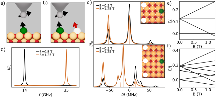
Figure 1: Scheme of the proposed STM-ESR experimental protocol. (a) Characterization of the bare resonance frequency $f_{0}$ of the sensor. (b) Determination of the $g$ coefficients of a single unit (atom) of the on-surface spin array. (c) ESR-STM readout of the bare sensor at two different fields. (d) ESR-STM readouts of a sensor nearby antiferromagnetically coupled dimer (top) and a trimer (bottom), with $J=124\mu$eV and $T=1$ K, using different magnetic fields that lead to different occupations of the states. (e) and (f) Energy spectra of the dimer and trimer as a function of $B$.

The interaction between the spins of interest and the external field is given by: ${\cal H}_{1}=-\sum_{\alpha}M_{\alpha}B_{\alpha}$. For spin-rotational invariant Hamiltonians that commute with the Zeeman operator, $[{\cal H}_{0},{\cal H}_{1}]=0$, the spin susceptibility and the statistical variance of the total magnetization, $\Delta M_{\alpha}^{2}$ are related by Wieśniak et al. (2005):

$$\chi_{\alpha}=\beta\Delta M_{\alpha}^{2}=\beta\left(\sum_{i,j}\langle m_{\alpha}^{i}m_{\alpha}^{j}\rangle-(\sum_{i}\langle m_{\alpha}^{i}\rangle)^{2}\right)$$ (3)

where $\beta=\frac{1}{k_{B}T}$ . The variance for an isolated spin satisfies $\sum_{\alpha}g_{\alpha}^{2}\Delta S_{\alpha}^{2}\geq g_{\rm min}^{2}S$ where $g_{\rm min}={\rm Min}(g_{x},g_{y},g_{z})$. For a multi-spin system it has been shownHofmann and Takeuchi (2003) that, for non-entangled states, the variance of total magnetization is at least as large as the sum over variances of individual magnetizations. We thus can write the equation:

$${\rm Tr}\,\chi=\sum_{\alpha}\chi_{\alpha}=\chi_{x}+\chi_{y}+\chi_{z}=$$

$$=\beta\sum_{\alpha}\left(\sum_{i,j}\langle m_{\alpha}^{i}m_{\alpha}^{j}\rangle-(\sum_{i}\langle m_{\alpha}^{i}\rangle)^{2}\right)\geq\frac{g_{\rm min}^{2}\mu_{B}^{2}S}{k_{B}T}N$$ (4)

where $N$ is the number of spins and $S$ is the spin quantum number ($S=\frac{1}{2},1,...$). Equation (4) generalizes the result derived by Wiesnak et al.Wieśniak et al. (2005) to the case of anisotropic $g$ factor, relevant for surface spinsFerrón et al. (2019), and constitutes the starting point to our proposed entanglement certification method. If the spin-susceptibilities are measured, and violate the inequality of eq. (4), the presence of entanglement is certified. Equation (4) is a sufficient condition for entanglement, but not necessary: entanglement may be present, but go un-noticed, if the susceptibility satisfies eq. (4).

We discuss now how to certify entanglement using a single STM-ESR-active atom, that will be used as a sensor, placed nearby the spin array of interest. Specifically, we consider the case of dimersYang et al. (2017); Kot et al. (2022) and trimersYang et al. (2021) of antiferromagnetically coupled $S=1/2$ spins on MgOYang et al. (2021), the canonical surface for STM-ESR. The choice of $S=1/2$ rules out single ion anisotropies. In the suppl. material we show how the role of dipolar interactions can be neglected in most cases. Examples of $S=1/2$ adsorbates deposited on MgO include TiH Yang et al. (2017, 2018, 2019); Seifert et al. (2020); Steinbrecher et al. (2021); Veldman et al. (2021); Kot et al. (2022), CuYang et al. (2018), dimers of alkali atomsKovarik et al. (2022) and even organic moleculesLutz et al. (2022).

The spectra of the dimer and trimer are shown in Figure 1(e,f) as a function of the applied field. The dimer shows a singlet ground state with wave function $\frac{1}{\sqrt{2}}\left(|\uparrow\downarrow\rangle-|\downarrow\uparrow\rangle\right)$ and a triplet of excited states $(S=1,S_{z})$. The $S=1,\,S_{z}=\pm 1$ are product states, whereas the $S=1,\,S_{z}=0$ is entangled. The trimer ground state is a $S=1/2$ doublet with wave functions:

$$|\frac{1}{2},+\frac{1}{2}\rangle=-\frac{1}{\sqrt{6}}\left(|\uparrow\uparrow\downarrow\rangle+|\downarrow\uparrow\uparrow\rangle\right)+\sqrt{\frac{2}{3}}|\uparrow\downarrow\uparrow\rangle$$ (5)

and an analogous formula for $|S=\frac{1}{2},S_{z}=-\frac{1}{2}\rangle$. Therefore, both structures, dimer and trimer, have entangled ground states. The lowest energy excited state, with excitation energy $J$, is also a $S=1/2$ doublet, whereas the highest energy multiplet has $S=3/2$ and excitation energy $\frac{3J}{2}$.

ExperimentsChoi et al. (2017) show that the ESR spectrum, i.e., the $I_{DC}(f)$ curve of the sensor adatom, under the influence of a nearby spin-array, can be described by:

$$I_{DC}(f)=\sum_{n}p_{n}L(f-f_{n})$$ (6)

where the sum runs over the eigenstates of the Hamiltonian of the spin array, $\left({\cal H}_{0}+{\cal H}_{1}\right)|n\rangle=E_{n}|n\rangle$, $L$ is a lorentzian curve centered around the resonant frequency $f=f_{n}$, given by the expression

$$f_{n}(\vec{r})=\frac{\mu_{B}}{h}\sqrt{\sum_{\alpha}\left[g_{\alpha}^{\rm sensor}(B_{\alpha}+b_{n,\alpha}(\vec{r}))\right]^{2}}$$ (7)

Here, $h=2\pi\hbar$, $g_{\alpha}^{\rm sensor}$ are the components of the gyromagnetic tensor of the sensor, $B_{\alpha}$ represents the the external field and $b_{n,\alpha}(\vec{r})$ is the $\alpha$ component of the the stray field generated by the spin-array in the state $n$. The vector is given by

$$\vec{b}_{n}(\vec{r})=\frac{\mu_{0}}{4\pi}\sum_{i=1,N}\frac{3(\vec{m}^{i}(n)\cdot\vec{d}^{i})\vec{d}^{i}}{(d^{i})^{5}}-\frac{\vec{m}^{i}(n)}{(d^{i})^{3}}$$ (8)

where $\vec{r}^{i}$ are the positions of the surface spins and $\vec{r}$ is the position of the sensor, $\vec{d}^{i}=\vec{r}-\vec{r}^{i}$ and $\vec{m}^{i}(n)$ is a vector given by with components by

$$m_{\alpha}^{i}(n)=-g_{\alpha}\mu_{B}\langle n|S_{\alpha}i|n\rangle$$ (9)

the encode the quantum-average magnetization of the atomic moments of the spin array for state $n$. Equation 6 implicitly assumes the absence of resonant spin-flip interactions between the sensor spin and the spin-array.

In Figure 1d we show the spectra for a sensor nearby a dimer and a trimer of antiferromagnetically coupled spins, in the presence of a external field along the $z$ direction, assuming a broadening $\Delta f=5\,\rm{MHz}$ Baumann et al. (2015). The frequency shift of the $n$ peak, with respect to the bare sensor, are governed by the stray field $\vec{b}_{n}(\vec{r})$ generated by that state. For the dimer, the ESR-spectrum shows a prominent peak, that has contributions from both the $S=0,\,S_{z}=0$ and $S=1,\,S_{z}=0$ states, whose stray field vanish. As a result, the prominent peak has the frequency of the bare sensor. The two smaller peaks, symmetrically located around the central peak, correspond to the $S=1,S_{z}=\pm 1$ states. In the case of the trimer up to eight different peaks appear in our simulation, as the different doublets generate states with different magnetization and stray field.

We now express the average magnetization and the susceptibility in terms of the occupations $p_{n}$ and the magnetic moment of each state, the two quantities that can be obtained from ESR-STM. For spin-rotational invariant systems, we write eq. (1) as:

$$\langle M_{\alpha}\rangle=\sum_{n}p_{n}M_{\alpha}(n)$$ (10)

where $p_{n}=\frac{1}{Z}e^{-\beta E_{n}}$ is the equilibrium occupation of the $n$ eigenstate and $M_{\alpha}(n)=-g_{\alpha}\mu_{B}S_{\alpha}(n)$, and $S_{\alpha}(n)$ is the (half-)integer projection of the total spin operator of the spin-array along the $\alpha$ direction. The susceptibility would be given by

$$\chi_{\alpha}=\sum_{n}\frac{dp_{n}}{dB_{\alpha}}M_{\alpha}(n).$$ (11)

The experimental protocol to determine the $p_{n}$ is the followingChoi et al. (2017). For an ESR spectrum with $N_{p}$ visible peaks, we obtain the ratios $r_{n}=\frac{I_{n}}{I_{0}}$ where $I_{0}$ corresponds to the largest peak that arises from a single state. For trimers, $I_{0}$ is the peak that arises from the ground state. For dimers, the ground state peak has also contributions from the $S=1,S_{z}=0$ state and therefore we normalize with respect to the $S=1,S_{z}=-1$ peak. It has been demonstrated Choi et al. (2017) that the ratio of thermal occupations is the same than the ratio of Boltzman factors $r_{n}=\frac{p_{n}}{p_{0}}=\frac{I_{n}}{I_{0}}$. Assuming that the peaks exhaust the occupations of the states, we obtain $p_{n}$ out of the ratios (see suppl. mat.)

The determination of the $M_{\alpha}(n)$ can be done in two ways. First, the (half-)integer values of $S_{\alpha}$ could be assigned by inspection of the ESR spectrum relying on the fact that the states with largest $S_{\alpha}$ have larger stray field. We have verifieddel Castillo and Fernández-Rossier the feasibility of a second approach where the readout of the ESR spectra is repeated with the sensor in different locations, mapping the stray field of every state in real space, and pulling out the atomic magnetization averages, inferring $M_{\alpha}(n)$ thereby.

The protocol to measure the spin susceptibility of a spin array has the following steps, that have to be implemented for the three orientations $\alpha=x,y,z$ of the external field: 1. The bare resonant frequencies for the sensor $f_{0\alpha}=\frac{\mu_{B}}{h}g_{\alpha}^{\rm sensor}B_{\alpha}$ (Figure 1a) are determined in the absence of the spin array.

2. The $g_{\rm min}$ for the individual spins that form the array are determined. If they are ESR-STM active, a conventional resonance experiment is carried out, for the three directions of the field. Otherwise, the nearby ESR-STM sensor atom can be used Choi et al. (2017).

3. The $M_{\alpha}(n)$ and $p_{n}$ are obtained as explained above, for two values of $B_{\alpha}^{(1)}$ and $B_{\alpha}^{(2)}$. This permits us to obtain $\langle M_{\alpha}(B_{\alpha}^{(1)})\rangle$ and $\langle M_{\alpha}(B_{\alpha}^{(2)})\rangle$ for both fields and $\chi_{\alpha}=\frac{\langle M_{\alpha}(B_{\alpha}^{(2)})\rangle-\langle M_{\alpha}(B_{\alpha}^{(1)})\rangle}{B_{\alpha}^{(2)}-B_{\alpha}^{(1)}}$ and compare to eq. (4) to establish the presence of entanglement.

In the top panels of figure 2 we show the spin susceptibility for dimers and trimers as a function of temperature, together with the EW boundary, assuming isotropic factors, $g_{\alpha}=2$. We define the temperature $T^{*}$, below which the trace of the susceptibility matrix is smaller than the entanglement witness limit, so that equation (4) is not satisfied, and therefore the presence of entanglement is certified. The $\rm{Tr}\,\chi(T)$ curves are very different for dimer and trimer. At low T, the dimer is in the singlet state and its susceptibility vanish. In contrast, the trimer with $J>>k_{B}T$, the excited states play no role and the spin susceptibility is governed by the two states of the $S=1/2$ ground state doublet.

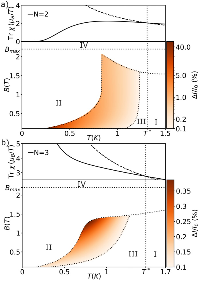
Figure 2: Entanglement certification window (see text) for a dimer (a) and trimer (b) with with $J=124\mu$eV, using a sensor located 0.9 nm away. Top panels show $\rm{Tr}\,\chi(T)$ and the EW condition of eq. (4). Color map inside the ECWs represents the largest experimental error $\Delta I/I_{0}$ that still makes entanglement certification possible, assuming $\eta=5$ in eq. 12.

The implementation of the entanglement certification protocol will only be possible if the stray fields induce a shift larger than the spectral resolution of ESR-STM. For ESR-STM , $\Delta f\simeq 4$MHzBaumann et al. (2015), determined by the $T_{1},T_{2}$ times of the adsorbate in that system. In the simulations of Figure 1 we have used $\Delta f=5MHz$. In addition, the experiment has to meet four experimental conditions. Condition $I$: temperature $T$ has to be smaller than $T^{*}$. Condition $II$: $M_{\alpha}(B_{\alpha})$ has to be linear. We define $B^{*}$ as the upper value of the field above which $\frac{dM_{\alpha}}{dB_{\alpha}}$ deviates from its value for $B=0$ more than 5 percent.

Condition $III$: the relative error in the current of the reference peak $\frac{\Delta I}{I_{0}}$ should be small enough to allow for the accurate entanglement certification. Specifically, the error in the spin susceptibility associated to $\frac{\Delta I}{I_{0}}$, should be smaller, by a factor $\eta>>1$, than the difference between $\chi_{\alpha}$ and the EW condition. In the suppl. mat. show this condition is

$$\frac{\Delta I}{I_{0}}<\frac{B|{\rm Tr\,}\chi-\chi_{EW}|}{6\eta p_{0}\sum_{n}\left(\left(2+r_{n}+(N_{p}-2)p_{0}\right)|M_{z}(n)|\right)}.$$ (12)

Condition $IV$: the external field must not drive the sensor resonant frequency above the excitation bandwidth of ESR-STM. The record, so far, is $f_{0}=61GHz$ Kot et al. (2022), that translates into $B\simeq 2.2$ T for $S=1/2$ Ti-H adsorbates.

The independent satisfaction of conditions $I$ to $IV$ occurs only in a region of the $(B,T)$ plane, defining four boundary lines, one per condition. We define the entanglement certification window (ECW) as the area where the four conditions are satisfied simultaneously. In Figure 2 we show the ECW, assuming $\eta=5$ and imposing for condition $III$ that $\Delta I/I_{0}$ can not go below $10^{-3}$, for the case of a dimer (a) and a trimer (b) with the same $J$ reported by Yang et al.Yang et al. (2021) $J=124\mu eV$ (30 GHz). The colour code signals the maximal $\Delta I/I_{0}$ that satisfies eq. (12).

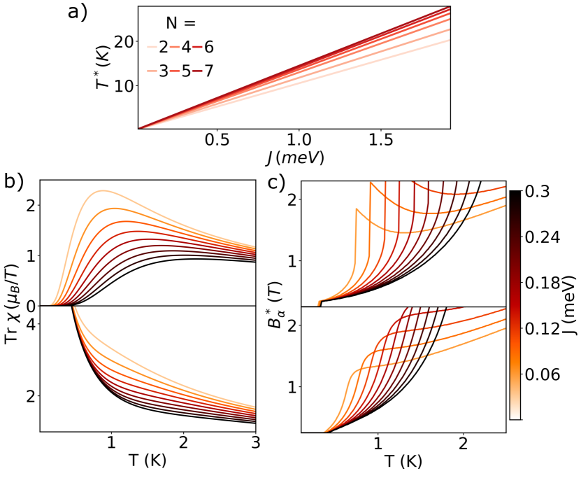
Figure 3: (a) $T^{*}(J)$ for different chain sizes.(b,c) Temperature and $J$ dependence of the spin susceptibility (b) and $B^{*}$ (c) of dimer (top) and trimer (bottom).

We now discuss the effect of the value of $J$ on the size of the ECW. In Figure 3a we show that $T^{*}$ is strictly linear with $J$ for spin chains with $N$ sites, and the slope is an increasing function of the number of $N$. Therefore, both long chains and large $J$ increase the crossover temperature. As of condition two, our numerical simulations show that $B^{*}$ is an increasing function of both $T$ and $J$: the magnetization vs field curves remain linear as long as the Zeeman energy is smaller than the other two relevant energy scales $J$ and $T$. Condition three is governed both by the ratio $B/p_{0}(B,T)$ (see eq. 12 ) and the susceptibility. In Figure 3b we show the $J$ dependence of the $\chi(T)$ curves. We see that reducing $J$ tends to increase $\chi$, at a fixed value of $T$. Again, this reflects the competition between exchange and Zeeman energies. Therefore, increasing $J$ pushes $T^{*}$ up and pushes the $\chi(T)$ away from the EW boundary. The only advantage of smaller values of $J/K_{B}T$ is the presence of more peaks in the $I(f)$ spectra that makes the spectra clearly distinguishable from simpler structures.

In conclusion, we propose a method to determine the presence of quantum entanglement in on-surface spin arrays using ESR-STM. For that matter, the trace of the spin susceptibility of the spin arrays has to be measured taking advantage of the STM potential i) to manipulate atoms and build spin structures, and ii) to simultaneously resolve the stray fields and occupation probabilities of several quantum states of nearby spinsChoi et al. (2017). Our calculations show that the experiments can be carried out with the state of the art ESR-STM instrumentation in terms of both spectral resolution ($\Delta f$) and relative error in the current $\Delta I/I_{0}$Choi et al. (2017). The use of STM to certify the presence of entanglement would thus add a new functionality to this versatile tool and would open a new venue in quantum nanoscienceHeinrich et al. (2021).

We acknowledge Antonio Costa for useful discussions. J.F.R. acknowledges financial support from FCT (Grant No. PTDC/FIS-MAC/2045/2021), SNF Sinergia (Grant Pimag), FEDER /Junta de Andalucía, (Grant No. P18-FR-4834), Generalitat Valenciana funding Prometeo2021/017 and MFA/2022/045, and funding from MICIIN-Spain (Grant No. PID2019-109539GB-C41). YDC acknowledges funding from FCT, QPI, (Grant No. SFRH/BD/151311/2021) and thanks the hospitality of the Departamento de Física Aplicada at the Universidad de Alicante.

References

- Bell and Bell (2004) J. S. Bell and J. S. Bell, Speakable and unspeakable in quantum mechanics: Collected papers on quantum philosophy (Cambridge university press, 2004).
- Bennett et al. (1993) C. H. Bennett, G. Brassard, C. Crépeau, R. Jozsa, A. Peres, and W. K. Wootters, Physical Review Letters 70, 1895 (1993).
- Bouwmeester et al. (1997) D. Bouwmeester, J.-W. Pan, K. Mattle, M. Eibl, H. Weinfurter, and A. Zeilinger, Nature 390, 575 (1997).
- Boschi et al. (1998) D. Boschi, S. Branca, F. De Martini, L. Hardy, and S. Popescu, Physical Review Letters 80, 1121 (1998).
- Kitaev and Preskill (2006) A. Kitaev and J. Preskill, Physical Review Letters 96, 110404 (2006).
- Nielsen and Chuang (2002) M. A. Nielsen and I. Chuang, “Quantum computation and quantum information,” (2002).
- Degen et al. (2017) C. L. Degen, F. Reinhard, and P. Cappellaro, Reviews of Modern Physics 89, 035002 (2017).
- Wootters (1998) W. K. Wootters, Philosophical Transactions of the Royal Society of London. Series A: Mathematical, Physical and Engineering Sciences 356, 1717 (1998).
- Friis et al. (2019) N. Friis, G. Vitagliano, M. Malik, and M. Huber, Nature Reviews Physics 1, 72 (2019).
- Heinrich et al. (2021) A. J. Heinrich, W. D. Oliver, L. M. Vandersypen, A. Ardavan, R. Sessoli, D. Loss, A. B. Jayich, J. Fernandez-Rossier, A. Laucht, and A. Morello, Nature Nanotechnology 16, 1318 (2021).
- Arnesen et al. (2001) M. Arnesen, S. Bose, and V. Vedral, Physical Review Letters 87, 017901 (2001).
- Amico and Fazio (2009) L. Amico and R. Fazio, Journal of Physics A: Mathematical and Theoretical 42, 504001 (2009).
- Hirjibehedin et al. (2006) C. F. Hirjibehedin, C. P. Lutz, and A. J. Heinrich, Science 312, 1021 (2006).
- Khajetoorians et al. (2019) A. A. Khajetoorians, D. Wegner, A. F. Otte, and I. Swart, Nature Reviews Physics 1, 703 (2019).
- Choi et al. (2019) D.-J. Choi, N. Lorente, J. Wiebe, K. Von Bergmann, A. F. Otte, and A. J. Heinrich, Reviews of Modern Physics 91, 041001 (2019).
- Delgado and Fernández-Rossier (2017) F. Delgado and J. Fernández-Rossier, Progress in Surface Science 92, 40 (2017).
- Chen et al. (2022) Y. Chen, Y. Bae, and A. J. Heinrich, Advanced Materials , 2107534 (2022).
- Mishra et al. (2021) S. Mishra, G. Catarina, F. Wu, R. Ortiz, D. Jacob, K. Eimre, J. Ma, C. A. Pignedoli, X. Feng, P. Ruffieux, J. Fernandez-Rossier, and R. Fasel, Nature 598, 287 (2021).
- Yang et al. (2021) K. Yang, S.-H. Phark, Y. Bae, T. Esat, P. Willke, A. Ardavan, A. J. Heinrich, and C. P. Lutz, Nature Communications 12, 1 (2021).
- Toskovic et al. (2016) R. Toskovic, R. Van Den Berg, A. Spinelli, I. Eliens, B. Van Den Toorn, B. Bryant, J.-S. Caux, and A. Otte, Nature Physics 12, 656 (2016).
- Wieśniak et al. (2005) M. Wieśniak, V. Vedral, and Č. Brukner, New Journal of Physics 7, 258 (2005).
- Brukner et al. (2006) Č. Brukner, V. Vedral, and A. Zeilinger, Physical Review A 73, 012110 (2006).
- Vedral (2008) V. Vedral, Nature 453, 1004 (2008).
- Sahling et al. (2015) S. Sahling, G. Remenyi, C. Paulsen, P. Monceau, V. Saligrama, C. Marin, A. Revcolevschi, L. Regnault, S. Raymond, and J. Lorenzo, Nature Physics 11, 255 (2015).
- Baumann et al. (2015) S. Baumann, W. Paul, T. Choi, C. P. Lutz, A. Ardavan, and A. J. Heinrich, Science 350, 417 (2015).
- Natterer et al. (2017) F. D. Natterer, K. Yang, W. Paul, P. Willke, T. Choi, T. Greber, A. J. Heinrich, and C. P. Lutz, Nature 543, 226 (2017).
- Choi et al. (2017) T. Choi, W. Paul, S. Rolf-Pissarczyk, A. J. Macdonald, F. D. Natterer, K. Yang, P. Willke, C. P. Lutz, and A. J. Heinrich, Nature Nanotechnology 12, 420 (2017).
- Hofmann and Takeuchi (2003) H. F. Hofmann and S. Takeuchi, Physical Review A 68, 032103 (2003).
- Ferrón et al. (2019) A. Ferrón, S. A. Rodríguez, S. S. Gómez, J. L. Lado, and J. Fernández-Rossier, Physical Review Research 1, 033185 (2019).
- Yang et al. (2017) K. Yang, Y. Bae, W. Paul, F. D. Natterer, P. Willke, J. L. Lado, A. Ferrón, T. Choi, J. Fernández-Rossier, A. J. Heinrich, et al., Physical Review Letters 119, 227206 (2017).
- Kot et al. (2022) P. Kot, M. Ismail, R. Drost, J. Siebrecht, H. Huang, and C. R. Ast, arXiv preprint arXiv:2209.10969 (2022).
- Yang et al. (2018) K. Yang, P. Willke, Y. Bae, A. Ferrón, J. L. Lado, A. Ardavan, J. Fernández-Rossier, A. J. Heinrich, and C. P. Lutz, Nature Nanotechnology 13, 1120 (2018).
- Yang et al. (2019) K. Yang, W. Paul, F. D. Natterer, J. L. Lado, Y. Bae, P. Willke, T. Choi, A. Ferrón, J. Fernández-Rossier, A. J. Heinrich, et al., Physical Review Letters 122, 227203 (2019).
- Seifert et al. (2020) T. S. Seifert, S. Kovarik, D. M. Juraschek, N. A. Spaldin, P. Gambardella, and S. Stepanow, Science Advances 6, eabc5511 (2020).
- Steinbrecher et al. (2021) M. Steinbrecher, W. M. Van Weerdenburg, E. F. Walraven, N. P. Van Mullekom, J. W. Gerritsen, F. D. Natterer, D. I. Badrtdinov, A. N. Rudenko, V. V. Mazurenko, M. I. Katsnelson, et al., Physical Review B 103, 155405 (2021).
- Veldman et al. (2021) L. M. Veldman, L. Farinacci, R. Rejali, R. Broekhoven, J. Gobeil, D. Coffey, M. Ternes, and A. F. Otte, Science 372, 964 (2021).
- Kovarik et al. (2022) S. Kovarik, R. Robles, R. Schlitz, T. S. Seifert, N. Lorente, P. Gambardella, and S. Stepanow, Nano Letters (2022).
- Lutz et al. (2022) C. Lutz, G. Czap, and M. Sherwood, Bulletin of the American Physical Society (2022).
- (39) Y. del Castillo and J. Fernández-Rossier, In preparation .