Causal Vector Auto-Regression Enhanced with Covariance and Order Selection

Abstract

A causal vector autoregressive (CVAR) model is introduced for weakly stationary multivariate processes, combining a recursive directed graphical model for the contemporaneous components and a vector autoregressive model longitudinally. Block Cholesky decomposition with varying block sizes is used to solve the model equations and estimate the path coefficients along a directed acyclic graph (DAG). If the DAG is decomposable, i.e. the zeros form a reducible zero pattern (RZP) in its adjacency matrix, then covariance selection is applied that assigns zeros to the corresponding path coefficients. Real life applications are also considered, where for the optimal order $p\geq 1$ of the fitted CVAR$(p)$ model, order selection is performed with various information criteria.

Keywords: Structural vector Auto-Regression; Causality along a DAG; Block Cholesky decomposition; Covariance selection; Order selection

PACS: J0101  MSC: 15B05; 62M10; 65F99; 65F30

1 Introduction

The purpose of this paper is to connect graphical modeling tools and time series models together via path coefficient estimation. In statistics, the path analysis was established by the geneticist Wright (1934) about a century ago, but he used complicated entrywise calculations with partial correlations. Taking these partial correlations of a pair of variables in a multidimensional data set conditioned on another set of variables, makes things overtly complicated, as the conditioning set changes in every step. A bit later, in econometrics, structural equation modeling (SEM) was developed; the prominent author Haavelmo (1943) obtained the Nobel price for it later. The maximum likelihood estimation (MLE) of the parameters in the Gaussian case was elaborated by Joreskog (1977). At the same time, Wold (1985), inventor of partial least squares regression (PLS), used matrix calculations, and Kiiveri et al. (1984) already used block matrix decompositions when dividing their variables into endogenous and exogenous ones. However, none of these authors applied steadily algorithms of block LDL (variant of the Cholesky) decomposition alone, without using partial correlations. Further, they did not consider time series.

Here we give a rigorous block matrix approach of these problems originated in statistics and time series analysis. Furthermore, we enhance the usual and structural vector autoregressive (VAR and SVAR) models, discussed e.g. in Deistler and Scherrer (2019) and Deistler and Scherrer (2022), with a causal component that has an effect between the coordinates contemporaneously. Therefore, we call our causal vector autoregressive model CVAR. Joint effects between the contemporaneous components are also considered in SVAR models of Keating (1996) and Lütkepohl (2005); Kilian and Lütkepohl (2017), but just recursive ordering of the variables, and no specific structure of the underlying directed graph is investigated. Though in Wold (1960) a causal chain model is introduced with an exogenous and a lagged endogenous variable, Gaussian Markov processes and usual regression estimates are used in context of econometrical problems. This research is also inspired by the paper Wermuth (1980), where recursive ordering of the variables is crucial, without using any time component.

Eichler (2016) introduces causality as a fundamental tool for the empirical investigations of dynamic interactions in multivariate time series. He also discusses the differences between the structural and Granger causality. Former one appears in the SVAR models (see Geweke (1984)), whereas the latter one first appears in Wiener (1956), then in Granger (1969), and is sometimes called Wiener–Granger causality. Without causality between the contemporaneous components, our model in the Gaussian case also resembles the one of Eichler (2012), where the error term (shock) can have correlated components. Our higher order recursive VAR model can be transformed into a model like this, but the price is loosing the recursive structure. The VAR model of Brillinger (1996) has a similar structure as ours with uncorrelated error terms; but no further benefits of recursive models, like RZP, induced by the underlying DAG, are discussed. Sims (1980) investigates the use of different type structural equation and autoregressive models in macroeconomy, without suggesting numerical algorithms. However, historically this survey paper was among the first ones which pointed out the difference between the so far existing macroeconomic models and distinguished endogenous and exogenous variables. The method of the most recent paper Bazinas and Nielsen (2022) is based on the reduced form system and is constructed by the conditional distribution of two endogenous variables, given a catalyst or multiple catalysts; lagged effects are assessed, without having a longer time series, and stationarity is not assumed.

Throughout the paper, second order processes are considered that can be assumed to follow multivariate Gaussian distribution. In Section 2, the different types of VAR models are compared, and a novel causal VAR model is introduced, combining the above recursive model contemporaneously and a VAR$(p)$ model longitudinally. In Section 3, the models are described in details, together with introducing algorithms for the parameter estimation. In Subsection 3.1, the unrestricted CVAR(1) model is introduced, while in Subsection 3.2, the restricted cases are treated, with some prescribed zeros in the path coefficients. Relation to covariance selection and decomposability is discussed too. In Subsection 3.3, higher order CVAR models are introduced. In Section 4, application to real life data is presented together with information criteria for order selection (optimal choice of $p$). The results and estimation schemes are summarized in Section 5; finally, in Section 6, conclusions and further perspectives are posed. The proofs of the theorems and the detailed description of the algorithms are to be found in Appendix A, while a survey about graphical models, with emphases to the Gaussian case, in Appendix B.

2 Materials & Methods

First the different purpose VAR$(p)$ models for the $d$-dimensional, weakly stationary process $\{\mathbf{X}_{t}\}$ are enlisted and compared. The first two models are known in the literature, whereas the last two ones are our contributions, for which block matrix decomposition based algorithms are introduced in Section 3, and they are illustrated in Section 4 on real life data.

• Reduced form VAR$(p)$ model: for given integer $p\geq 1$, it is

  $$\mathbf{X}_{t}+\bm{M}_{1}\mathbf{X}_{t-1}+\dots+\bm{M}_{p}\mathbf{X}_{t-p}=\mathbf{V}_{t},\quad t=p+1,p+2,\dots,$$ (1)

  where $\mathbf{V}_{t}$ is white noise, it is uncorrelated with $\mathbf{X}_{t-1},\dots,\mathbf{X}_{t-p}$, it has zero expectation and covariance matrix $\bm{\Sigma}$ (not necessarily diagonal, but positive definite), and the matrices $\bm{M}_{j}$ satisfy the stability conditions (see Deistler and Scherrer (2019)). (Sometimes $\mathbf{X}_{t}$ is isolated on the left hand side.) $\mathbf{V}_{t}$ is called innovation, i.e. the error term of the (added value to the) best one-step ahead linear prediction of $\mathbf{X}_{t}$ with its past, which (in case of a VAR($p$) model) can be done with the $p$-lag long past $\mathbf{X}_{t-1},\dots,\mathbf{X}_{t-p}$.

• Structural form SVAR$(p)$ model: for given integer $p\geq 1$, it is

  $$\bm{A}\mathbf{X}_{t}+\bm{B}_{1}\mathbf{X}_{t-1}+\dots+\bm{B}_{p}\mathbf{X}_{t-p}=\mathbf{U}_{t},\quad t=p+1,p+2,\dots,$$ (2)

  where the white noise term $\mathbf{U}_{t}$ is uncorrelated with $\mathbf{X}_{t-1},\dots,\mathbf{X}_{t-p}$, it has zero expectation with uncorrelated components, i.e. with positive definite, diagonal covariance matrix $\bm{\Delta}$. $\bm{A}$ is $d\times d$ upper triangular matrix with 1s along its main diagonal; whereas, $\bm{B}_{1},\dots,\bm{B}_{p}$ are $d\times d$ matrices, see also Lütkepohl (2005).

  There is a one-to-one correspondence between the reduced and structural model; since $\bm{A}$ is invertible, from Equation (2), Equation (1) can be obtained (and vice versa):

  $$\mathbf{X}_{t}+{\bm{A}}^{-1}\bm{B}_{1}\mathbf{X}_{t-1}+\dots+{\bm{A}}^{-1}\bm{B}_{p}\mathbf{X}_{t-p}={\bm{A}}^{-1}\mathbf{U}_{t},\quad t=p+1,p+2,\dots,$$

  where $\bm{M}_{j}={\bm{A}}^{-1}\bm{B}_{j}$, $\mathbf{V}_{t}={\bm{A}}^{-1}\mathbf{U}_{t}$, and $\bm{\Sigma}={\bm{A}}^{-1}\bm{\Delta}{{\bm{A}}^{T}}^{-1}$; further, $|\bm{\Sigma}|=|\bm{\Delta}|$ as $|\bm{A}|=1$.

  Note that if the ordering of the components of $\mathbf{X}_{t}$ is changed (with some permutation of $\{1,\dots,d\}$), then the rows of the matrices $\bm{M}_{j}$, further, the rows and columns of $\bm{\Sigma}$ are permuted accordingly. However, the matrices $\bm{A}$, $\bm{B}_{j}$ and $\bm{\Delta}$ cannot be obtained in this simple way, they profoundly change under the above permutation.

• Causal CVAR$(p)$ unrestricted model: it also obeys Equation (2), but here the ordering of the components follows a causal ordering, given e.g. by an expert knowledge. This is a recursive ordering along a “complete” DAG, where the permutation (labeling) of the graph nodes (assigned to the components of $\mathbf{X}_{t}$) is such that $X_{t,i}$ can be caused by $X_{t,j}$ whenever $i<j$, which means a $j\to i$ directed edge. Here the causal effects are meant contemporaneously, and reflected in the upper triangular structure of the matrix $\bm{A}$.

  It is important that in any ordering of the jointly Gaussian variables, a Bayesian network or a Gaussian directed graphical model can be constructed, in which every node (variable) is regressed linearly with the variables corresponding to higher label nodes, see Appendix B. The partial regression coefficients behave like path coefficients, also used in SEM. If the DAG is complete, then there are no zero constraints imposed on the partial regression coefficients.

• Causal CVAR$(p)$ restricted model: here an incomplete DAG is built, based on partial correlations, but in the conditioning set the $p$-lag long past also counts.

  First we build an undirected graph: not connect $i$ and $j$ if the partial correlation coefficient of $X_{i}$ and $X_{j}$, eliminating the effect of the other variables is 0 (theoretically), or less than a threshold (practically). Such an undirected graphical model is called Markov random field (RMF). It is known (see Rao (1973) and Lauritzen (2004)) that partial correlations can be calculated from the concentration matrix (inverse of the covariance matrix). But here the upper left block of the inverse of the large block matrix, containing the first $p$ autocovariance matrices, is used. If this undirected graph is triangulated, then in a convenient (so-called perfect) ordering of the nodes, the zeros of the adjacency matrix form an RZP. We can find such an ordering (not necessarily unique) with the maximal cardinality search (MCS) algorithm, together with cliques and separators of a so-called junction tree (JT), see Bolla et al. (2019) and Appendix B. In this ordering (labeling) of the nodes, a DAG can also be constructed, which is Markov equivalent to the undirected one (it has no so-called sink V configuration), for further details see Subsection 3.2.

  Observe that in this DAG, in the Gaussian case, the fact that for $i<j$: $X_{i}$ and $X_{j}$ are conditionally independent given $\{i+1,\dots,d\}\setminus\{j\}$ is equivalent to the fact that $X_{i}$ and $X_{j}$ are conditionally independent given all the remaining components. (It does not mean that the regression or partial correlation coefficients are the same, just they are zeros at the same time.)

  Having an RZP in the CVAR restricted model, we use the incomplete DAG for estimation. With the covariance selection method of Dempster (1972), the starting concentration matrix is re-estimated by imposing zero constraints for its entries in the RZP positions (symmetrically). By the theory (see, e.g. Bolla et al. (2019)), this will result in zero entries of $\bm{A}$ in the no directed edge positions. This also becomes obvious from Appendix B and the algorithm of the Appendix A.4.

Note that the unrestricted CVAR model can as well use an incomplete DAG, where the labeling of its nodes follows the perfect labeling of the undirected graph; still, the parameter matrices $\bm{A}$ and $\bm{B}_{j}$s are “full” in the sense that no zeros of $\bm{A}$ are guaranteed in the no-edge positions of the graph. Their entries are just considered as path coefficients of the contemporaneous and lagged effects, respectively. On the contrary, in the restricted CVAR model, action is done for introducing zero entries in $\bm{A}$ in the no-edge positions. If the desired zeros form an RZP, the covariance selection has a closed form (see Lauritzen (2004)). In the lack of an RZP, the covariance selection also works, but it needs an infinite (convergent) iteration, called Iterative Proportional Scaling (IPS), see Appendix B.

Then both in the unrestricted and restricted CVAR$(p)$ models an order selection is initiated to choose the optimal $p$, based on information criteria, like AIC, BIC, AICC, and HQ, where only the number of parameters differs in the two cases. Actually, in the restricted case, the covariances are estimated only within the cliques and separators of the JT, which can reduce the computational complexity of our algorithm when the number of nodes is “large”.

3 Results

3.1 The Unrestricted Causal VAR(1) Model

The directed Gaussian graphical model of Wermuth (1980) (see Appendix B.6) does not consider time development; it is, in fact, a CVAR(0) model. Also note that at this point, the ordering of the jointly Gaussian variables is not relevant, since in any recursive ordering of them (encoded in $\bm{A}$) a Gaussian directed graphical model (in other words, a Gaussian Bayesian network) can be constructed, where every variable is regressed linearly with the higher label ones. This is due to the solvability of the recursive equation system (B.4) with the LDL decomposition (B.6) in any ordering of the rows and columns of $\bm{\Sigma}$.

To introduce the unrestricted CVAR(1) model, let $\{\mathbf{X}_{t}\}$ be a $d$-dimensional, weakly stationary process with real valued components of zero expectation and covariance matrix function $\bm{C}(h)$, $h=0,\pm 1,\pm 2,\dots$; $\bm{C}(-h)=\bm{C}^{T}(h)$. All deterministic and random vectors are column vectors and so, $\bm{C}(h)=\mathbb{E}\mathbf{X}_{t}\mathbf{X}_{t+h}^{T}$ does not depend on $t$, by weak stationarity. The model equation is

$$\bm{A}\mathbf{X}_{t}+\bm{B}\mathbf{X}_{t-1}=\mathbf{U}_{t},\quad t=1,2,\dots,$$ (3)

where $\bm{A}$ is $d\times d$ upper triangular matrix with 1s along its main diagonal, $\bm{B}$ is a $d\times d$ matrix; further, the white noise random vector $\mathbf{U}_{t}$ is uncorrelated with (in the Gaussian case, independent of) $\mathbf{X}_{t-1}$, has zero expectation and covariance matrix $\bm{\Delta}=\mathrm{diag}(\delta_{1},\dots,\delta_{d})$.

Let $\mathfrak{C}_{2}$ denote the covariance matrix of the stacked random vector $(\mathbf{X}^{T}_{t},\mathbf{X}^{T}_{t-1})^{T}$ which, in block matrix form, is as follows:

$$\mathfrak{C}_{2}=\begin{pmatrix}\bm{C}(0)&\bm{C}^{T}(1)\\ \bm{C}(1)&\bm{C}(0)\end{pmatrix}.$$ (4)

It is symmetric and positive definite if the process is of full rank regular (which means that its spectral density matrix of Bolla and Szabados (2021) is of full rank) that is assumed in the sequel. It is well known that the inverse of $\mathfrak{C}_{2}$, the so-called concentration matrix $\bm{K}$, has the block-matrix form

$$\bm{K}=\begin{pmatrix}\bm{C}^{-1}(1|0)&-\bm{C}^{-1}(1|0)\bm{C}^{T}(1)\bm{C}^{-1}(0)\\ -\bm{C}^{-1}(0)\bm{C}(1)\bm{C}^{-1}(1|0)&\bm{C}^{-1}(0)+\bm{C}^{-1}(0)\bm{C}(1)\bm{C}^{-1}(1|0)\bm{C}^{T}(1)\bm{C}^{-1}(0)\end{pmatrix},$$

where $\bm{C}(1|0)=\bm{C}(0)-\bm{C}^{T}(1)\bm{C}^{-1}(0)\bm{C}(1)$ is the conditional covariance matrix $\bm{C}(t|t-1)$ of the distribution of $\mathbf{X}_{t}$ conditioned on $\mathbf{X}_{t-1}$; by weak stationarity, it does not depend on $t$ either, therefore it is denoted by $\bm{C}(1|0)$. Also, $\mathfrak{C}_{2}$ is positive definite if and only if both $\bm{C}(0)$ and $\bm{C}(1|0)$ are positive definite.

Observe that $\bm{C}(1|0)=\bm{A}^{-1}\bm{\Delta}{\bm{A}^{-1}}^{T}$ is the covariance matrix of the innovation $\mathbf{V}_{t}={\bm{A}}^{-1}\mathbf{U}_{t}$. Therefore, the left upper block of $\bm{K}$ contains its inverse, which is $\bm{A}^{T}\bm{\Delta}^{-1}\bm{A}$.

Theorem 1

The parameter matrices $\bm{A}$, $\bm{B}$, and $\bm{\Delta}$ of model Equation (3) can be obtained by the block LDL decomposition of the (positive definite) concentration matrix $\bm{K}$ (inverse of the covariance matrix $\mathfrak{C}_{2}$ in Equation (4)) of the $2d$-dimensional Gaussian random vector $(\mathbf{X}^{T}_{t},\mathbf{X}^{T}_{t-1})^{T}$. If $\bm{K}=\bm{L}\bm{D}\bm{L}^{T}$ is this (unique) decomposition with block-triangular matrix $\bm{L}$ and block-diagonal matrix $\bm{D}$, then they have the form

$$\bm{L}=\begin{pmatrix}\bm{A}^{T}&\bm{O}_{d\times d}\\ \bm{B}^{T}&\bm{I}_{d\times d}\end{pmatrix},\qquad\bm{D}=\begin{pmatrix}\bm{\Delta}^{-1}&\bm{O}_{d\times d}\\ \bm{O}_{d\times d}&\bm{C}^{-1}(0)\end{pmatrix},$$ (5)

where the $d\times d$ upper triangular matrix $\bm{A}$ with 1s along its main diagonal, the $d\times d$ matrix $\bm{B}$, and the diagonal matrix $\bm{\Delta}$ of model Equation (3) can be retrieved from them.

The proof of this theorem together with the detailed description of the algorithm is to be found in Sections A.1 and A.2 of Appendix A.

3.2 The Restricted Causal VAR(1) Model

Assume that we have a causal ordering of the coordinates $X_{1},\dots,X_{d}$ of $\mathbf{X}$ such that $X_{j}$ can be the cause of $X_{i}$ whenever $i<j$. We can think of $X_{i}$s as the nodes of a graph in a directed graphical model (Bayesian network) and their labeling corresponds to a topological ordering of the nodes of the underlying DAG. So $i<j$ can imply an $i\to j$ edge, and then we say that $X_{j}$ is a parent (cause) of $X_{i}$ ($X_{i}$ can have multiple parents, maximum $d-i$ ones), see Section B.1. For example, when asset prices or relative returns of different assets or currencies (on the same day) influence each other in a certain (recursive) order. Now, restricted cases are analyzed, when only certain arrows (causes) are present, but the DAG is connected. In particular, only certain asset prices influence some others on a DAG contemporaneously, but not all possible directed edges are present. In this case, a covariance selection technique can be initiated to re-estimate the covariance matrix so that the partial regression coefficients in the no-edge positions be zeros.

When the DAG is built from an undirected graph, then we also require that the so constructed DAG be Markov equivalent to its undirected skeleton. Then the DAG must not contain sink V configuration (see the forthcoming Remark 1), which fact is equivalent to having a so-called RZP (see Wermuth (1980)) in the adjacency matrix of the undirected graph in the DAG labeling (also see the forthcoming Definition 2). In this case, the positions of the zero entries in the concentration matrix are identical to the positions of the zero entries in $\bm{A}$. More exactly, for $i=1,\dots,d-1$ and $j=i+1,\dots,d$: $\beta_{ij\cdot\{i+1,\dots,d\}}$, the partial regression coefficient of $X_{j}$ when regressing $X_{i}$ with $X_{i+1},\dots,X_{d}$, is zero exactly when $r_{ij\cdot\{1,\dots,d\}\setminus\{i,j\}}$ (the partial correlation coefficient between $X_{i}$ and $X_{j}$, excluding the effect of all other variables) is zero. In other wording, if the DAG does not contain sink V configuration, then it is Markov equivalent to it undirected skeleton, see Lauritzen (2004) and Corollary 1 of Appendix B.3.

In the sequel, we will consider these so-called decomposable cases, though there are algorithms, like the Iterative Proportional Scaling (IPS) for the general case too. About the relation of the directed and undirected cases, and equivalent notions of decomposability, e.g. existence of a junction tree (JT) structure, see Appendix B.3.

In the unrestricted model, no restrictions for the upper-diagonal entries of $\bm{A}$ were made. In practice, we have a sample and all the autocovariance matrices are estimated, and the resulting $\bm{A},\bm{B}$ matrices are calculated with them. Usually a statistical hypothesis testing advances this procedure, during which it can be found that certain partial correlations (closely related to the entries of $\bm{K}$) do not significantly differ from zero. Then we naturally want to introduce zeros for the corresponding entries of $\bm{A}$. For this, the method of covariance selection of Dempster (1972) is elaborated, see also Lauritzen (2004), Wermuth (1980), and Appendix B.5, from which we recall the following notions here.

Definition 1

Let $\bm{M}$ be the adjacency matrix of an undirected graph on node set labelled as $\{1,\dots,d\}$; i.e. for $i\neq j$: $m_{ij}=m_{ji}=1$ if $i\sim j$ ($i$ and $j$ are connected) and 0, otherwise (the diagonal entries are zeros). We say that $\bm{M}$ has a reducible zero pattern (RZP) if $m_{ij}=0$ $(i<j)$ implies that for each $h=1,\dots,i-1$: either $m_{hi}=0$ or $m_{hj}=0$ holds (or both hold). (This applies to the entries above the main diagonal and symmetrically extends to those below the main diagonal: $m_{ij}=m_{ji}$ for $j<i$.)

Definition 2

Let $\bm{M}$ be the adjacency matrix of a DAG in the topological ordering $1,\dots,d$ of its nodes; i.e. for $i<j$: $m_{ij}=1$ if there is a $j\to i$ edge and 0, otherwise ($\bm{M}$ is upper triangular with zero diagonal). We say that $\bm{M}$ has a reducible zero pattern (RZP) if $m_{ij}=0$ $(i<j)$ implies that for each $h=1,\dots,i-1$: either $m_{hi}=0$ or $m_{hj}=0$ holds (or both hold).

Remark 1

Obviously, in the adjacency matrix of a DAG, an RZP is present if and only if there is no sink V configuration in the topological ordering of the DAG. Under sink V configuration a triplet $j\rightarrow h\leftarrow i$ is understood, where $i$ is not connected by $j$ (see Figure 2 of Appendix B.1). Indeed, in this case the DAG has a triplet $h<i<j$ with $m_{hj}\neq 0$, $m_{hi}\neq 0$, but $m_{ij}=0$, in contrast to Definition 2.

Observe that the RZP applies only to the positions of the zero entries of a matrix. So we are able to give a more general definition.

Definition 3

Let $\bm{M}$ be a symmetric or an upper triangular matrix of real entries. We say that $\bm{M}$ has a reducible zero pattern (RZP) if $m_{ji}=0$ $(j<i)$ implies that for each $h=1,\dots,j-1$: either $m_{hj}=0$ or $m_{hi}=0$ holds (or both hold).

In view of this, we can find relation between the zeros of $\bm{A}$ in the CVAR(1) model and those of the inverse covariance matrix.

Proposition 1

The upper triangular matrix $\bm{A}$ of model equation (3) has an RZP if and only if the upper left $d\times d$ block of $\bm{K}=\mathfrak{C}_{2}^{-1}$ has an RZP. Moreover, the zero entries of $\bm{A}$ are exactly in the same positions as the zero entries of the upper diagonal part of the upper left block of $\bm{K}$.

Proof 1

In one direction, the proof follows from Equation (A.4) of Section A.2 in Appendix A. Indeed, in presence of an RZP in $\bm{A}$, for $1\leq j<i\leq d$: if $l_{ij}(=a_{ji})=0$, then $k_{ij}=0$, since either $\ell_{ih}(=a_{hi})=0$ or $\ell_{jh}(=a_{hj})=0$ (or both) for $h=1,\dots,j-1$, which are the intrinsic entries of the summation in Equation (A.4).

In the other direction, if $k_{ij}=0$, then $l_{ij}=a_{ji}=0$ too, because of the Markov equivalence of the DAG and its undirected skeleton in the decomposable case; see Corollary 1 of Appendix B.3. Here we use that $k_{ij}$ and $l_{ij}$ are positive constant multiples of partial correlation and partial regression coefficients.

Consequently, if we have causal relations between the contemporaneous components of $\mathbf{X}_{t}$, and the so constructed DAG has an RZP, then this RZP is inherited by the left upper block of $\bm{K}$, which is $\bm{C}^{-1}(1|0)$. Therefore, we further improve the covariance selection model Dempster (1972), by introducing zero entries into the sample conditional covariance matrix. Actually, fixing the zero entries in the left upper block of $\bm{K}$, we re-estimate the matrix $\mathfrak{C_{2}}$. In the possession of a sample, there are exact MLE estimates developed for this purpose (see Bolla et al. (2019), Lauritzen (2004)).

Assume that the cliques of the node set $\{1,\dots,d\}$ of $\mathbf{X}_{t}$ are $C_{1},\dots,C_{k}$, to which a last clique is added, formed by the components $X_{t-1,1},\dots,X_{t-1,d}$ of $\mathbf{X}_{t-1}$. If $C_{1},\dots,C_{k}$ form a JT in this ordering, the joint density of $\mathbf{X}_{t}$ and $\mathbf{X}_{t-1}$ factorizes like

$$f(\mathbf{x}_{t},\mathbf{x}_{t-1})=f(\mathbf{x}_{t-1})\prod_{j=1}^{k}f(\mathbf{x}_{t,R_{j}}\,|\,\mathbf{x}_{t,S_{j}},\mathbf{x}_{t-1}).$$

For covariance selection, we include the lag 1 variables $X_{t-1,1},\dots,X_{t-1,d}$ too. Therefore, the new cliques and separators are

$$C^{\prime}_{j}:=C_{j}\cup\{X_{t-1,1},\dots,X_{t-1,d}\},\quad j=1,\dots,k$$

and

$$S^{\prime}_{j}:=S_{j}\cup\{X_{t-1,1},\dots,X_{t-1,d}\},\quad j=2,\dots,k.$$

Having this, we are able to re-estimate the $2d\times 2d$ $\bm{K}$, inverse of $\mathfrak{C}_{2}$ in (4), for our VAR(1) model as follows:

$${\hat{\bm{K}}}=(n-1)\left\{\sum_{j=1}^{k}[\bm{S}_{C^{\prime}_{j}}^{-1}]^{2d}-\sum_{j=2}^{k}[\bm{S}_{S^{\prime}_{j}}^{-1}]^{2d}\right\},$$ (6)

where the matrix $\bm{S}_{C^{\prime}}$ is the usual product-moment estimate based on the $n-1$ element sample with the following variables:

$$\left(X_{t,i}:\,i\in C\quad\textrm{and}\quad X_{t-1,1},\dots,X_{t-1,d}\right),\quad t=2,\dots,n;$$

further, $[\bm{M}_{C^{\prime}}]^{2d}$ denotes the $2d\times 2d$ matrix comprising the entries of the larger $2d\times 2d$ matrix $\bm{M}$ in the $|C^{\prime}|\times|C^{\prime}|$ block corresponding to $C^{\prime}$, and otherwise zeros. By the properties of the LDL decomposition, these zeros go into zeros of $\bm{A}$. For illustrations, see Section 4 and B.5.

Note that for the MLE, here we do not have an i.i.d. sample, but a serially correlated sample. However, by ergodicity, for “large” $n$, this choice also works and gives an asymptotic MLE, akin to the product-moment estimates.

3.3 Higher Order Causal VAR Models

The above model can be further generalized to the following recursive VAR($p$) model: for given integer $p\geq 1$,

$$\bm{A}\mathbf{X}_{t}+\bm{B}_{1}\mathbf{X}_{t-1}+\dots+\bm{B}_{p}\mathbf{X}_{t-p}=\mathbf{U}_{t},\quad t=p+1,p+2,\dots,$$ (7)

where the white noise term $\mathbf{U}_{t}$ is uncorrelated with $\mathbf{X}_{t-1},\dots,\mathbf{X}_{t-p}$, it has zero expectation and covariance matrix $\bm{\Delta}=\mathrm{diag}(\delta_{1},\dots,\delta_{d})$. $\bm{A}$ is $d\times d$ upper triangular matrix with 1s along its main diagonal; whereas, $\bm{B}_{1},\dots,\bm{B}_{p}$ are $d\times d$ matrices.

Here we have to perform the block Cholesky decomposition of the inverse covariance matrix of $(\mathbf{X}_{t}^{T},\mathbf{X}_{t-1}^{T},\dots,\mathbf{X}_{t-p}^{T})^{T}$, i.e. the inverse of the matrix

$$\mathfrak{C}_{p+1}=\left(\begin{array}[]{lllll}\bm{C}(0)&\bm{C}^{T}(1)&\bm{C}^{T}(2)&\cdots&\bm{C}^{T}(p)\\ \bm{C}(1)&\bm{C}(0)&\bm{C}^{T}(1)&\cdots&\bm{C}^{T}(p-1)\\ \bm{C}(2)&\bm{C}(1)&\bm{C}(0)&\cdots&\bm{C}^{T}(p-2)\\ \vdots&\vdots&\vdots&\ddots&\vdots\\ \bm{C}(p)&\bm{C}(p-1)&\bm{C}(p-2)&\cdots&\bm{C}(0)\\ \end{array}\right).$$ (8)

This is a symmetric, positive definite block Toeplitz matrix with $(p+1)\times(p+1)$ blocks which are $d\times d$ matrices. Again, $\bm{C}^{T}(h)=\bm{C}(-h)$ and it is well known that the inverse matrix $\mathfrak{C}_{p+1}^{-1}$ has the following block-matrix form:

• Upper left block: $\bm{C}^{-1}(p|0,\dots,p-1)$;

• Upper right block: $-\bm{C}^{-1}(p|0,\dots,p-1)\bm{C}^{T}(1,\dots,p)\mathfrak{C}_{p}^{-1}$;

• Lower left block: $-\mathfrak{C}_{p}^{-1}\bm{C}(1,\dots,p)\bm{C}^{-1}(p|0,\dots,p-1)$;

• Lower right block: $\mathfrak{C}_{p}^{-1}+\mathfrak{C}_{p}^{-1}\bm{C}(1,\dots,p)\bm{C}^{-1}(p|0,\dots,p-1)\bm{C}^{T}(1,\dots,p)\mathfrak{C}_{p}^{-1}$,

where $\bm{C}(p|0,\dots,p-1)=\bm{C}(0)-\bm{C}^{T}(1,\dots,p)\mathfrak{C}_{p}^{-1}\bm{C}(1,\dots,p)$ is the conditional covariance matrix $\bm{C}(t|t-1,\dots,t-p)$ of the distribution of $\mathbf{X}_{t}$ given $\mathbf{X}_{t-1},\dots,\mathbf{X}_{t-p}$; due to stationarity, it does not depend on $t$ either, therefore it is denoted by $\bm{C}(p|0,\dots,p-1)$. Further, $\bm{C}^{T}(1,\dots,p)=(\bm{C}^{T}(1),\dots,\bm{C}^{T}(p))$ is $d\times pd$ and $\bm{C}(1,\dots,p)$ is $pd\times d$. Also, $\mathfrak{C}_{p+1}$ is positive definite if and only if both $\mathfrak{C}_{p}$ and $\bm{C}(p|0,\dots,p-1)$ are positive definite.

Theorem 2

The parameter matrices $\bm{A}$, $\bm{B}_{1},\dots,\bm{B}_{p}$ and $\bm{\Delta}$ of model Equation (7) can be obtained by the block LDL decomposition of the (positive definite) concentration matrix $\bm{K}$ (inverse of the covariance matrix $\mathfrak{C}_{p+1}$ in Equation (8)) of the $(p+1)d$-dimensional Gaussian random vector $(\mathbf{X}_{t}^{T},\mathbf{X}_{t-1}^{T},\dots,\mathbf{X}_{t-p}^{T})^{T}$. If $\bm{K}=\bm{L}\bm{D}\bm{L}^{T}$ is this (unique) decomposition with block-triangular matrix $\bm{L}$ and block-diagonal matrix $\bm{D}$, then they have the form

$$\bm{L}=\begin{pmatrix}\bm{A}^{T}&\bm{O}_{d\times pd}\\ \bm{B}^{T}&\bm{I}_{pd\times pd}\end{pmatrix},\qquad\bm{D}=\begin{pmatrix}\bm{\Delta}^{-1}&\bm{O}_{d\times pd}\\ \bm{O}_{pd\times d}&\mathfrak{C}_{p}^{-1}\end{pmatrix},$$ (9)

where the $d\times d$ upper triangular matrix $\bm{A}$ with 1s along its main diagonal, the $d\times pd$ matrix $\bm{B}=(\bm{B}_{1}\dots\bm{B}_{p})$ (transpose of $\bm{B}^{T}$, partitioned into blocks) and the diagonal matrix $\bm{\Delta}$ of model Equation (7) can be retrieved from them.

The proof of this theorem together with the detailed description of the algorithm is to be found in Sections A.3 and A.4 of Appendix A.

Restricted cases can be treated similarly as in Section 3.2. Here too, the existence of an RZP in the DAG on $d$ nodes is equivalent to the existence of an RZP in the left upper $d\times d$ corner of the concentration matrix $\mathfrak{C}_{p+1}^{-1}$. From the model equations it is obvious that

$$X_{t,i}=-\sum_{j=i+1}^{d}a_{ij}X_{t,j}-\sum_{h=1}^{p}\sum_{j=1}^{d}b_{h,ij}X_{t-h,j}-U_{t,i},$$

where $X_{t,i}$ is the $i$th coordinate of $\mathbf{X}_{t}$. By weak stationarity it follows that the entries of the matrices $\bm{A}$ and $\bm{B}_{h}=(b_{h,ij})_{i,j=1}^{p}$ are partial regression coefficients as follows:

$$a_{ij} =-\beta_{X_{t,i}X_{t,j}\cdot\{X_{t,i+1},\dots,X_{t,d},X_{t-1,1},\dots,X_{t-1,d},\dots,X_{t-p,1},\dots,X_{t-p,d}\}},\quad 1\leq i<j\leq d;$$

$$b_{h,ij} =-\beta_{X_{t,i}X_{t+h,j}\cdot\{X_{t,i+1},\dots,X_{t,d},X_{t-1,1},\dots,X_{t-1,d},\dots,X_{t-p,1},\dots,X_{t-p,d}\}},$$

$$1\leq i<j\leq d,\quad h=1,\dots,d.$$

Since the conditioning set changes from equation to equation, it is easier to use the block LDL decompositions here, without the exact meaning of the coefficients.

Considering the components of $\mathbf{X}_{t},\mathbf{X}_{t-1},\dots,\mathbf{X}_{t-p}$ as nodes of the expanded graph, the joint density of $\mathbf{X}_{t},\mathbf{X}_{t-1},\dots,\mathbf{X}_{t-p}$ factorizes like

$$f(\mathbf{x}_{t},\mathbf{x}_{t-1},\dots,\mathbf{x}_{t-p}) =f(\mathbf{x}_{t-1},\dots,\mathbf{x}_{t-p})f(\mathbf{x}_{t}\,|\,\mathbf{x}_{t-1},\dots,\mathbf{x}_{t-p})$$

$$=f(\mathbf{x}_{t-1},\dots,\mathbf{x}_{t-p})\cdot\prod_{i=1}^{d}f(x_{t,i}\,|\,\mathbf{x}_{t,\,\mathrm{par}(i)},\mathbf{x}_{t-1},\dots,\mathbf{x}_{t-p}).$$

Now assume that the cliques of the node set $\{1,\dots,d\}$ of $\mathbf{X}_{t}$ are $C_{1},\dots,C_{k}$ (as at the end of Section 3.2) and they form a JT with residuals $R_{1},\dots,R_{k}$ and separators $S_{1},\dots,S_{k}$ (with the understanding that $S_{1}=\emptyset$ and $R_{1}=C_{1}$). Enhancing the preceding density with this, we get the following factorization:

$$f(\mathbf{x}_{t},\mathbf{x}_{t-1},\dots,\mathbf{x}_{t-p})=f(\mathbf{x}_{t-1},\dots,\mathbf{x}_{t-p})\cdot\prod_{j=1}^{k}f(\mathbf{x}_{t,R_{j}}\,|\,\mathbf{x}_{t,S_{j}},\mathbf{x}_{t-1},\dots,\mathbf{x}_{t-p}).$$

Covariance selection can be done similarly as in Section 3.2, but here zero entries of the left upper $d\times d$ block of $\mathfrak{C}_{p+1}^{-1}$ provide the zero entries of $\bm{A}$. For this purpose, the $n-p$ element sample entries are used with the following coordinates:

$$\left(X_{t,i}:\,i\in C\quad\textrm{and}\quad X_{t-1,1},\dots,X_{t-1,d},\dots,X_{t-p,1},\dots,X_{t-p,d}\right),$$

for $t=p+1,\dots,n$ when we calculate the product-moment estimate $\bm{S}_{C^{\prime}}$ with $C^{\prime}=C\cup\{\mathbf{X}_{t-1},\dots,\mathbf{X}_{t-p}\}$. For more details see the explanation after Equation (6) and Section 4.

Note that here the covariance selection is done based only on a serially correlated and not an independent sample. However, when $n$ is “large”, then ergodicity issues (see, e.g. Bolla and Szabados (2021)) give rise to this relaxation of the original algorithm. Also, by the theory of Brockwell and Davis (1991) (p. 424), it is guaranteed that the Yule-Walker equations have a stable stationary solution to the VAR$(p)$ model, whenever the starting covariance matrix of $(p+1)\times(p+1)$ blocks is positive definite. But we assume this in our theorems. In this case, the empirical versions are also positive definite (almost surely as $n\to\infty$), and the covariance selection also gives a positive definite estimate. So the estimated parameter matrices provide a stable VAR model in view of the theory and ergodicity if $n$ is “large”.

4 Applications with Order Selection

4.1 Financial Data

We used the data communicated in the the paper Akbilgic et al. (2014) on daily relative returns of 8 different asset prices, spanning 534 days. The multivariate time series was found stationary and nearly Gaussian.

First we applied the unrestricted CVAR($p$) model. We constructed a DAG by making the undirected graph on 8 nodes directed. The undirected graph was constructed by testing statistical hypotheses for the partial correlations of the pairs of the variables conditioned on all the others. As the test statistic is increasing in the absolute value of the partial correlation in question, a threshold 0.04 for the latter one was used that corresponds to significance level $\alpha=0.008851$ of the partial correlation test. Table 1 contains the partial correlations based on $\bm{C}^{-1}(0)$.

	NIK	EU	ISE	EM	BVSP	DAX	FTSE	SP
NIK		0.016∗	0.035∗	0.522	-0.260	-0.019∗	-0.076	0.024∗
EU	0.016∗		0.217	0.034∗	0.067	0.687	0.747	0.018∗
ISE	0.035∗	0.217		0.358	-0.157	-0.077	-0.059	0.034∗
EM	0.522	0.034∗	0.358		0.546	0.048	0.086	-0.184
BVSP	-0.260	0.067	-0.157	0.546		-0.093	-0.045	0.533
DAX	-0.019∗	0.687	-0.077	0.048	-0.093		-0.203	0.191
FTSE	-0.076	0.747	-0.059	0.086	-0.045	-0.203		0.057
SP	0.024∗	0.018∗	0.034∗	-0.184	0.533	0.191	0.057

Table 1: Partial Correlation Coefficients from $\bm{C}^{-1}(0)$. Entries marked by asterisk are less than 0.04 in absolute value (i.e. they correspond to no-edge positions in the graph), the corresponding significance is $\alpha=0.008851$.

Since the graph was triangulated, with the MCS algorithm, we were able to (not necessarily uniquely) label the nodes so that the adjacency matrix of this undirected graph had an RZP:

$$1:\,\textrm{NIK (stock market return index of Japan)},$$

$$2:\,\textrm{EU (MSCI European index)},$$

$$3:\,\textrm{ISE (Istanbul stock exchange national 100 index)}$$

$$4:\,\textrm{EM (MSCI emerging markets index)},$$

$$5:\,\textrm{BVSP (stock market return index of Brazil)},$$

$$6:\,\textrm{DAX (stock market return index of Germany)},$$

$$7:\,\textrm{FTSE (stock market return index of UK)},$$

$$8:\,\textrm{SP (Standard \& poor's 500 return index)}.$$

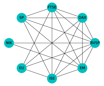
(a) MRF fitted to the financial dataset.

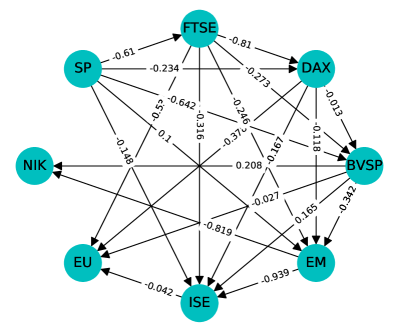
(b) DAG oriented in the MCS ordering.

Figure 1: Graphical models fitted to the financial dataset

If this is considered as the topological labeling of the DAG, where directed edges point from a higher label node to a lower label one, then the so obtained directed graph is Markov equivalent to its undirected skeleton, see Figures 1a and 1b. But the RZP is used only in the restricted case, in the unrestricted case only the DAG ordering of the variables is used.

We ran the VAR($p$) algorithm with $p=1,2,3,4,5$ and found that the $\bm{A}$ matrices do not change much with increasing $p$, akin to $\bm{B}_{1}$. The $\bm{B}_{2},..,\bm{B}_{5}$ matrices have relatively “small” entries. Consequently, contemporaneous effects and one-day lags are the most important. This is also supported by the forthcoming order selection investigations. For the $p=1$ and $p=2$ cases, see Tables 2,3 and 4,5,6, respectively.

	NIK	EU	ISE	EM	BVSP	DAX	FTSE	SP
NIK	1	0.0264	0.0042	-0.8902	0.2030	0.0170	0.0781	-0.0336
EU	0	1	-0.0418	-0.0146	-0.0239	-0.3746	-0.5255	-0.0033
ISE	0	0	1	-0.9518	0.1613	-0.1658	-0.3129	-0.1413
EM	0	0	0	1	-0.3507	-0.1182	-0.2464	0.1077
BVSP	0	0	0	0	1	-0.0129	-0.2782	-0.6375
DAX	0	0	0	0	0	1	-0.8102	-0.2336
FTSE	0	0	0	0	0	0	1	-0.6100
SP	0	0	0	0	0	0	0	1

Table 2: $\bm{A}$ for the unrestricted Financial VAR(1) model (rounded to 4 decimals).

	NIK-1	EU-1	ISE-1	EM-1	BVSP-1	DAX-1	FTSE-1	SP-1
NIK	0.1845	-0.1685	-0.0874	0.0852	0.0635	0.0205	-0.1236	-0.2798
EU	-0.0131	0.1219	-0.0044	0.0291	-0.0124	-0.0393	-0.0979	0.0011
ISE	0.0677	0.2811	-0.0657	0.2473	-0.2940	-0.0543	0.0098	-0.1442
EM	-0.0016	-0.0569	-0.0159	0.1076	-0.0917	-0.0945	0.0875	-0.1071
BVSP	-0.0140	0.0704	0.0142	-0.1046	0.1397	-0.1497	0.1188	-0.0812
DAX	-0.0034	0.2021	-0.0342	-0.0044	-0.0352	-0.0476	-0.0670	-0.0673
FTSE	0.0293	-0.0168	-0.0109	0.0420	-0.1129	0.2141	0.0805	-0.2641
SP	0.0417	0.2603	-0.0261	0.0112	-0.0026	-0.0709	-0.2850	0.1240

Table 3: $\bm{B}$ for the unrestricted Financial VAR(1) model (rounded to 4 decimals).

	NIK	EU	ISE	EM	BVSP	DAX	FTSE	SP
NIK	1	-0.0114	0.0103	-0.8822	0.1995	0.0233	0.0856	-0.0214
EU	0	1	-0.0426	-0.0110	-0.0240	-0.3745	-0.5137	-0.0128
ISE	0	0	1	-0.9788	0.1701	-0.1669	-0.3139	-0.1361
EM	0	0	0	1	-0.3450	-0.1154	-0.2375	0.0922
BVSP	0	0	0	0	1	-0.0047	-0.2655	-0.6601
DAX	0	0	0	0	0	1	-0.8120	-0.2339
FTSE	0	0	0	0	0	0	1	-0.6320
SP	0	0	0	0	0	0	0	1

Table 4: $\bm{A}$ for the unrestricted Financial VAR(2) model (rounded to 4 decimals).

	NIK-1	EU-1	ISE-1	EM-1	BVSP-1	DAX-1	FTSE-1	SP-1
NIK	0.2063	-0.1826	-0.1106	0.1063	0.0731	0.0187	-0.1502	-0.2580
EU	-0.0037	0.1364	-0.0010	0.0232	-0.0150	-0.0371	-0.0996	-0.0107
ISE	0.0409	0.2476	-0.0771	0.2274	-0.2772	-0.0447	0.0331	-0.1284
EM	0.0489	-0.0200	-0.0030	0.1360	-0.1150	-0.0996	0.0468	-0.1162
BVSP	-0.0066	0.0931	0.0261	-0.1091	0.1312	-0.1573	0.1161	-0.0935
DAX	-0.0123	0.2146	-0.0319	0.0073	-0.0406	-0.0536	-0.0727	-0.0694
FTSE	0.0852	0.0019	0.0275	0.0145	-0.1117	0.2377	0.1035	-0.3427
SP	0.0530	0.2759	-0.0565	-0.0033	0.0024	-0.0945	-0.3106	0.1789

Table 5: $\bm{B_{1}}$ for the unrestricted Financial VAR(2) model (rounded to 4 decimals).

	NIK-2	EU-2	ISE-2	EM-2	BVSP-2	DAX-2	FTSE-2	SP-2
NIK	-0.0402	-0.1695	-0.0410	0.0156	0.0998	-0.0406	0.1367	-0.0091
EU	0.0017	0.0771	-0.0065	0.0054	0.0037	0.0192	-0.0762	-0.0394
ISE	-0.0142	-0.1725	-0.0276	-0.0088	0.0389	0.1167	0.0826	0.0357
EM	-0.0054	0.0650	-0.0322	0.1155	-0.0695	-0.0959	-0.0162	-0.0270
BVSP	-0.0423	0.0332	-0.0449	0.2878	-0.0717	-0.0221	-0.0381	-0.0120
DAX	-0.0372	0.0177	0.0130	0.0658	-0.0360	-0.0108	-0.0202	0.0059
FTSE	0.0491	0.3107	-0.0820	0.0693	0.0299	0.0153	-0.0840	-0.3038
SP	0.0447	-0.0628	0.0804	-0.1824	0.0785	0.0133	-0.1775	0.1284

Table 6: $\bm{B_{2}}$ for the unrestricted Financial VAR(2) model (rounded to 4 decimals).

Then we considered the restricted CVAR(1) model. Here we want to introduce structural zeros into the matrix $\bm{A}$. Now the matrix $C^{-1}(1|0)$, the left upper $8\times 8$ corner of $\mathfrak{C}_{2}^{-1}$ is used for covariance selection. Figure 1b shows this DAG with the significant path coefficients above the arrows, based on Table 7.

The ordering of the variables is the same as in the unrestricted case, but the RZP is a bit different. The decomposable structure has the following cliques and separators:

$$C_{1} =\{\textrm{BVSP,DAX,EM,FTSE,ISE,SP}\}=\{3,4,5,6,7,8\}$$ (10)

$$C_{2} =\{\textrm{BVSP,DAX,EU,FTSE,ISE}\}=\{2,3,5,6,7\}$$

$$C_{3} =\{\textrm{BVSP,EM,NIK}\}=\{1,4,5\}$$

$$S_{2} =\{\textrm{BVSP,DAX,FTSE,ISE}\}=\{3,5,6,7\}$$

$$S_{3} =\{\textrm{BVSP,EM}\}=\{4,5\},$$

where the parent clique of both $C_{2}$ and $C_{3}$ is $C_{1}$. Note, that the set of nodes in the second braces is the same, but they follow increasing labels so that better see the JT structure. variables too;

The matrices $\bm{A}$ and $\bm{B}$ were estimated via the algorithm for the LDL decomposition of $\hat{\bm{K}}$. Here the zeros of the left upper $8\times 8$ block of $\hat{\bm{K}}$ will necessarily result in the zeros of $\bm{A}$ in the same positions. The upper-diagonal entries of $\bm{A}$ and the entries of $\bm{B}$ are considered as path coefficients which represent the contemporaneous and 1-day lagged effect of the assets to the others, respectively; see Table 7 and Table 8.

	NIK	EU	ISE	EM	BVSP	DAX	FTSE	SP
NIK	1	0	0	-0.8193	0.2080	0	0	0
EU	0	1	-0.0421	0	-0.0269	-0.3782	-0.5297	0
ISE	0	0	1	-0.9386	0.1653	-0.1675	-0.3161	-0.1477
EM	0	0	0	1	-0.3419	-0.1184	-0.2464	0.0997
BVSP	0	0	0	0	1	-0.0130	-0.2729	-0.6423
DAX	0	0	0	0	0	1	-0.8102	-0.2336
FTSE	0	0	0	0	0	0	1	-0.6104
SP	0	0	0	0	0	0	0	1

Table 7: $\bm{A}$ matrix for the restricted Financial VAR(1) model (rounded to 4 decimal places).

	NIK-1	EU-1	ISE-1	EM-1	BVSP-1	DAX-1	FTSE-1	SP-1
NIK	0.1811	-0.1797	-0.0856	0.0842	0.0739	-0.0058	-0.1146	-0.2662
EU	-0.0131	0.1213	-0.0046	0.0304	-0.0130	-0.0415	-0.0969	0.0002
ISE	0.0676	0.2814	-0.0658	0.2483	-0.2941	-0.0567	0.0120	-0.1472
EM	-0.0016	-0.0567	-0.0158	0.1067	-0.0908	-0.0951	0.0890	-0.1085
BVSP	-0.0139	0.0704	0.0142	-0.1041	0.1391	-0.1488	0.1195	-0.0828
DAX	-0.0034	0.2019	-0.0342	-0.0046	-0.0353	-0.0474	-0.0669	-0.0672
FTSE	0.0292	-0.0171	-0.0109	0.0419	-0.1130	0.2142	0.0807	-0.2642
SP	0.0417	0.2608	-0.0261	0.0115	-0.0026	-0.0713	-0.2853	0.1239

Table 8: $\bm{B}$ matrix for the restricted Financial VAR(1) model (rounded to 4 decimal places).

In the VAR(2) situation, the graph, constructed by $C^{-1}(2|1,0)$ is the same, has the same JT with 3 cliques and the same RZP as based on $C^{-1}(1|0)$. It is in accord with our former observation that the lag 2 or more days effects of the assets to the others is negligible compared to the 1-day lag effect (the forthcoming order selection also supports this).

Here the $24\times 24$ matrix $\hat{\bm{K}}$ was estimated by adapting Equation (6) to the $3d\times 3d$ situation, by using both the lag 1 and lag 2 variables for covariance selection. The estimated $\bm{A},\bm{B}_{1}$, and $\bm{B}_{2}$ matrices are shown in Tables 9, 10, and 11.

	NIK	EU	ISE	EM	BVSP	DAX	FTSE	SP
NIK	1	0	0	-0.8191	0.2076	0	0	0
EU	0	1	-0.0423	0	-0.0293	-0.3811	-0.5192	0
ISE	0	0	1	-0.9662	0.1790	-0.1713	-0.3112	-0.1470
EM	0	0	0	1	-0.3361	-0.1153	-0.2372	0.0835
BVSP	0	0	0	0	1	-0.0069	-0.2544	-0.6664
DAX	0	0	0	0	0	1	-0.8128	-0.2336
FTSE	0	0	0	0	0	0	1	-0.6319
SP	0	0	0	0	0	0	0	1

Table 9: $\bm{A}$ matrix for the restricted Financial VAR(2) model (rounded to 4 decimals).

	NIK-1	EU-1	ISE-1	EM-1	BVSP-1	DAX-1	FTSE-1	SP-1
NIK	0.2009	-0.1869	-0.1098	0.1089	0.0824	-0.0079	-0.1493	-0.2428
EU	-0.0038	0.1387	-0.0013	0.0260	-0.0153	-0.0410	-0.1027	-0.0086
ISE	0.0353	0.2865	-0.0750	0.2479	-0.2741	-0.0639	0.0101	-0.1418
EM	0.0494	-0.0218	-0.0027	0.1338	-0.1144	-0.0990	0.0500	-0.1177
BVSP	-0.0107	0.1202	0.0276	-0.0947	0.1327	-0.1674	0.0987	-0.1030
DAX	-0.0110	0.2072	-0.0322	0.0034	-0.0412	-0.0503	-0.0677	-0.0675
FTSE	0.0824	0.0176	0.0281	0.0224	-0.1104	0.2309	0.0928	-0.3463
SP	0.0506	0.2898	-0.0560	0.0040	0.0037	-0.1010	-0.3199	0.1760

Table 10: $\bm{B_{1}}$ matrix for the restricted Financial VAR(2) model (rounded to 4 decimals).

	NIK-2	EU-2	ISE-2	EM-2	BVSP-2	DAX-2	FTSE-2	SP-2
NIK	-0.0455	-0.1847	-0.0391	0.0264	0.0906	-0.0486	0.1427	0.0089
EU	0.0017	0.0755	-0.0058	0.0047	0.0033	0.0179	-0.0765	-0.0370
ISE	-0.0161	-0.1634	-0.0290	-0.0021	0.0352	0.1113	0.0821	0.0313
EM	-0.0056	0.0659	-0.0330	0.1189	-0.0701	-0.0959	-0.0167	-0.0283
BVSP	-0.0430	0.0415	-0.0456	0.2906	-0.0729	-0.0258	-0.0389	-0.0168
DAX	-0.0369	0.0163	0.0130	0.0656	-0.0356	-0.0100	-0.0203	0.0064
FTSE	0.0485	0.3142	-0.0820	0.0716	0.0290	0.0128	-0.0845	-0.3054
SP	0.0442	-0.0606	0.0805	-0.1825	0.0778	0.0117	-0.1773	0.1281

Table 11: $\bm{B_{2}}$ matrix for the restricted Financial VAR(2) model (rounded to 4 decimals).

To find the optimal order $p$, information criteria are suggested, see e.g. Box et al. (2015); Brockwell and Davis (1991). Here the following criteria will be used: the AIC (Akaike Information Criterion), the AICC (bias corrected version of the AIC), the BIC (Bayesian information criterion), and the HQ (Hannan and Quinn’s criterion). Each criterion can be decomposed into two terms: an information term that quantifies the information brought by the model (via the likelihood) and a penalization term that penalizes too “large” number of parameters, to avoid over-fitting. It can be proven that the AIC has a positive probability of overspecification and the BIC is strongly consistent, but sometimes it underspecifies the true model. The explicit forms of AIC, BIC, and HQ, which are to be minimized with respect to $p$, are as follows:

$$\textrm{AIC}(p) =\ln|{\hat{\bm{\Delta}}}|+\frac{2\left[pd^{2}+\binom{d}{2}\right]}{n-p}=\sum_{j=1}^{d}\ln{\hat{\delta}}_{j}+\frac{2\left[pd^{2}+\binom{d}{2}\right]}{n-p},$$

$$\textrm{BIC}(p) =\ln|{\hat{\bm{\Delta}}}|+\frac{\left[pd^{2}+\binom{d}{2}\right]\ln(n-p)}{n-p}=\sum_{j=1}^{d}\ln{\hat{\delta}}_{j}+\frac{\left[pd^{2}+\binom{d}{2}\right]\ln(n-p)}{n-p},$$

$$\textrm{HQ}(p) =\ln|{\hat{\bm{\Delta}}}|+\frac{2\left[pd^{2}+\binom{d}{2}\right]\ln(\ln(n-p))}{n-p}=\sum_{j=1}^{d}\ln{\hat{\delta}}_{j}+\frac{2\left[pd^{2}+\binom{d}{2}\right]\ln(\ln(n-p))}{n-p},$$

where $\hat{\bm{\Delta}}$ is the estimate of the error covariance matrix $\bm{\Delta}$.

The AICC (Akaike Information Criterion Corrected) is a bias-corrected version of Akaike’s AIC, which is an estimate of the Kullback-Leibler index of the fitted model relative to the true model and needs further explanation. Here

$$\textrm{AICC}(p)=-2\ln L({\hat{\bm{A}}},{\hat{\bm{B}}}_{1},\dots,{\hat{\bm{B}}}_{p},{\hat{\bm{\Delta}}})+\textrm{penalty}(p),$$

where the first term is $-2$ times the log-likelihood function, evaluated at the parameter estimates of Theorems 1 and 2, whereas the second term penalizes the computational complexity. The model parameters $\bm{A},\bm{B}_{1},\dots,\bm{B}_{p}$, and $\bm{\Delta}$ are estimated by the block Cholesky decomposition of the estimated inverse covariance matrix $\mathfrak{C}_{p+1}^{-1}$ of the Gaussian random vector $(\mathbf{X}_{t}^{T},\mathbf{X}_{t-1}^{T},\dots,\mathbf{X}_{t-p}^{T})^{T}$, see Algorithms A.2 and A.4. This is a moment estimation, but since our underlying distribution is multivariate Gaussian, which belongs to the exponential family, asymptotically, it is also an MLE (for “large” $n$) that satisfies the moment matching equations, see Wainwright and Jordan (2008). Of course, the matrices ${\hat{\bm{A}}},{\hat{\bm{B}}}_{1},\dots,{\hat{\bm{B}}}_{p}$, and ${\hat{\bm{\Delta}}}$ also depend on $p$, but for simplicity, we do not denote this dependence. More exactly,

$$L({\hat{\bm{A}}},{\hat{\bm{B}}}_{1},\dots,{\hat{\bm{B}}}_{p},{\hat{\bm{\Delta}}}) =(2\pi)^{-\frac{(n-p)d}{2}}|{\hat{\bm{\Delta}}}|^{-\frac{n-p}{2}}e^{-\frac{1}{2}\sum_{t=p+1}^{n}\mathbf{U}_{t}^{T}{\hat{\bm{\Delta}}}^{-1}\mathbf{U}_{t}}$$

$$=(2\pi)^{-\frac{(n-p)d}{2}}(\prod_{j=1}^{d}{\hat{\delta}}_{j})^{-\frac{n-p}{2}}e^{-\frac{1}{2}\sum_{t=p+1}^{n}\sum_{j=1}^{d}(U_{tj}^{2}/{\hat{\delta}}_{j})},$$

where

$$\mathbf{U}_{t}={\hat{\bm{A}}}(\mathbf{X}_{t}-{\hat{\mathbf{X}}}_{t}),$$

and

$${\hat{\mathbf{X}}}_{t}=-{\hat{\bm{A}}}^{-1}{\hat{\bm{B}}}_{1}\mathbf{X}_{t-1}-\dots-{\hat{\bm{A}}}^{-1}{\hat{\bm{B}}}_{p}\mathbf{X}_{t-p},$$

for $t=p+1,\dots,n$.

In the unrestricted model, the complexity term (see Brockwell and Davis (1991)) is

$$\frac{2\left[pd^{2}+\binom{d}{2}\right](n-p)d}{(n-p)d-pd^{2}-\binom{d}{2}-1}.$$

Therefore,

$$\textrm{AICC}(p)=(n-p)d\ln(2\pi)+(n-p)\ln|{\hat{\bm{\Delta}}}|+\sum_{t=p+1}^{n}\mathbf{U}^{T}{\hat{\bm{\Delta}}}^{-1}\mathbf{U}_{t}+\frac{2\left[pd^{2}+\binom{d}{2}\right](n-p)d}{(n-p)d-pd^{2}-\binom{d}{2}-1}$$

$$=(n-p)d\ln(2\pi)+(n-p)\sum_{j=1}^{d}\ln{\hat{\delta}}_{j}+\sum_{t=p+1}^{n}\sum_{j=1}^{d}\frac{U_{tj}^{2}}{{\hat{\delta}}_{j}}+\frac{2\left[pd^{2}+\binom{d}{2}\right](n-p)d}{(n-p)d-pd^{2}-\binom{d}{2}-1}.$$

In the restricted model, the penalization term depends on the cardinalities of the cliques $C_{1},\dots,C_{k}$ and those of the separators $S_{2},\dots,S_{k}$ that are the same for all $p$. The penalization terms for the four criteria are

$$\textrm{penalty}_{\textrm{AIC}}(p) =\frac{2\left[pd^{2}+\sum_{j=1}^{k}\binom{|C_{j}|}{2}+\sum_{j=2}^{k}\binom{|S_{j}|}{2}\right]}{n-p},$$

$$\textrm{penalty}_{\textrm{BIC}}(p) =\frac{\left[pd^{2}+\sum_{j=1}^{k}\binom{|C_{j}|}{2}+\sum_{j=2}^{k}\binom{|S_{j}|}{2}\right]\ln(n-p)}{n-p},$$

$$\textrm{penalty}_{\textrm{HQ}}(p) =\frac{2\left[pd^{2}+\sum_{j=1}^{k}\binom{|C_{j}|}{2}+\sum_{j=2}^{k}\binom{|S_{j}|}{2}\right]\ln(\ln(n-p))}{n-p}$$

$$\textrm{penalty}_{\textrm{AICC}}(p) =\frac{2\left[pd^{2}+\sum_{j=1}^{k}\binom{|C_{j}|}{2}+\sum_{j=2}^{k}\binom{|S_{j}|}{2}\right](n-p)d}{(n-p)d-pd^{2}-\sum_{j=1}^{k}\binom{|C_{j}|}{2}-\sum_{j=2}^{k}\binom{|S_{j}|}{2}-1}.$$

The cliques are usually of “small” sizes that can reduce computational complexity, but only when the number of variables $d$ is much “larger” than the clique sizes. In the financial model, with merely $d=8$ variables, the number of parameters is not smaller in the restricted case than in the unrestricted one, but the gain can be substantial with $d$ larger than, say, 100. Also this number of parameters to be estimated in the decomposable model is the same as the number of product moments calculated for the covariance selection, only within the cliques and separators, see Equation (B.3).

All of these criteria are tested, for both the restricted and unrestricted CVAR$(p)$ models, using the financial data above for $p=1,2,\dots,9$. The results for the unrestricted case are shown in Table 12.

$p$	AIC	AICC	BIC	HQ
1	-76.81	-33222.68	-76.07	-76.52
2	-76.85	-33173.98	-75.60	-76.36
3	-76.84	-33095.75	-75.08	-76.15
4	-76.83	-33011.98	-74.55	-75.94
5	-76.77	-32893.23	-73.97	-75.67
6	-76.69	-32766.33	-73.37	-75.39
7	-76.58	-32612.38	-72.74	-75.08
8	-76.48	-32457.38	-72.11	-74.77
9	-76.41	-32316.33	-71.52	-74.49

Table 12: Order selection criteria for the unrestricted Financial CVAR$(p)$ model, bold-face values represent minimum of each criterion.

Observe that in the unrestricted case, AIC reaches the minimum for $p=2$, whereas AICC, BIC, and HQ for $p=1$. This is in accord with our previous experience that the parameter matrices did not change much after the first or second day.

$p$	AIC	AICC	BIC	HQ
1	-76.82	-33224.46	-76.02	-76.51
2	-76.85	-33175.16	-75.55	-76.34
3	-76.88	-33114.07	-75.06	-76.17
4	-76.94	-33068.80	-74.61	-76.03
5	-76.89	-32952.72	-74.03	-75.77
6	-76.86	-32852.10	-73.49	-75.54
7	-76.76	-32700.55	-72.86	-75.23
8	-76.75	-32594.18	-72.32	-75.01
9	-76.72	-32476.45	-71.78	-74.79

Table 13: Order selection criteria for the restricted Financial CVAR$(p)$ model, bold-face values represent minimum of each criterion.

In the restricted case (see Table 13), except for the AIC, every criteria suggests that the best model is obtained with $p=1$. So the parameter matrices did not change much after the first day, except for AIC, which seems to overspecify the model and was the lowest on the 4th day, i.e. the last workday after the first workday.

4.2 IMR (Infant Mortality Rate) Longitudinal Data

Here, we used the longitudinal data of six indicators (components of $\mathbf{X}_{t}$), spanning 21 years ($1995-2015$) from the World Bank in case of Egypt:

$$1:\,\textrm{IMR (Infant mortality rate)},$$ (11)

$$2:\,\textrm{MMR (Maternal mortality ratio)},$$

$$3:\,\textrm{HepB (Hepatitis-B immunization)},$$

$$4:\,\textrm{GDP (Gross domestic per capita)},$$

$$5:\,\textrm{OPExp (Out-of-pocket health expenditure as \% of HExp)},$$

$$6:\,\textrm{HExp (Current health expenditure as \% of GDP)}.$$

For more details about these indicators, see Abdelkhalek and Bolla (2020). Through the VAR($p$) model, we show the contemporaneous and lag time effects between the components. Since the sample size is small, we investigate only VAR($1$) model in the unrestricted and restricted situations. Further, the variables are measured on different scales; so, we use the autocorrelations which are the autocovariances of the standardized variables. We distinguish between two working hypotheses with respect to two different ordering of the variables given by an expert:

• Case 1: $\{\textrm{IMR,MMR,HepB,OPExp,HExp ,GDP}\}$.

• Case 2: $\{\textrm{IMR,MMR,HepB,GDP,OPExp , HExp}\}$.

In the unrestricted CVAR(1) model, both orderings work, but we present only Case 1. (The estimated matrices $\bm{A}$ and $\bm{B}$ are mostly the same in both cases but the entries are interchanged with respect to the ordering of the variables.) The entries of matrix $\bm{A}$ (see Table 14) represent the contemporaneous effects (path coefficients) between the components at time $t$. The MMR has the largest contemporaneous inverse causal effect on the IMR, i.e. an increase in the MMR caused a decrease in the IMR by $1.13$. Matrix $\bm{B}$ (see Table 15), on the other hand, indicates the path coefficients of the one time lag causal effect of $\mathbf{X}_{t-1}$ on the current $\mathbf{X}_{t}$ components. An increase in the IMR at one year time lag caused an increase in the IMR at the current time by $0.29$. All other path coefficients in the matrices $\bm{A},\bm{B}$ can be explained likewise.

	IMR	MMR	HepB	OPExp	HExp	GDP
IMR	1.0	-1.1259	-0.0161	0.0003	0.0176	-0.1348
MMR	0.0	1.0000	0.3594	0.0492	-0.0684	0.7135
HepB	0.0	0.0000	1.0000	-0.1626	0.2510	-0.8196
OPExp	0.0	0.0000	0.0000	1.0000	-0.6876	-0.4229
HExp	0.0	0.0000	0.0000	0.0000	1.0000	0.6749
GDP	0.0	0.0000	0.0000	0.0000	0.0000	1.0000

Table 14: $\bm{A}$ matrix for the IMR unrestricted VAR($1$) model of Case 1 (rounded to $4$ decimals).

	IMR-1	MMR-1	HepB-1	OPExp-1	HExp-1	GDP-1
IMR	0.2986	-0.3589	-0.0076	0.0042	-0.0115	-0.0639
MMR	-0.0149	-0.7469	-0.2358	0.0540	0.0193	-0.5577
HepB	13.0541	-15.7658	-1.1915	-0.3506	0.2170	-1.7902
OPExp	7.1616	-8.0906	-0.2994	-0.1038	-0.0215	-0.7720
HExp	1.6861	-2.9922	-0.4650	-0.1566	-0.0681	-1.0913
GDP	-11.0674	13.2182	0.3254	0.3204	-0.3099	1.2129

Table 15: $\bm{B}$ matrix for the IMR unrestricted VAR($1$) model of Case 1 (rounded to $4$ decimals).

In the restricted CVAR(1) model, the graph structure is important. We consider only Case $2$ that provides the RZP and corresponds to the ordering of (11). Note that the so obtained DAG is Markov equivalent to its undirected skeleton. The decomposable structure of the JT has two cliques and only one separator as follows:

$$C_{1} =\{\textrm{IMR,MMR,HepB3,GDP,HExp}\}=\{1,2,3,4,6\},$$

$$C_{2} =\{\textrm{OPExp,HExp}\}=\{5,6\},$$

$$S_{2} =\{\textrm{HExp}\}=\{6\}.$$

In this case, the $n-1$ element sample including lag 1 variables is used to estimate the $12\times 12$ matrix $\hat{\bm{K}}$ with covariance selection, see Equation (6). Then the LDL algorithm was applied to the obtained $\hat{\bm{K}}$ to estimate the model parameters $\bm{A},\bm{B}$. Unlike the unrestricted model, here there are prescribed zero entries in $\hat{\bm{K}}$ and $\bm{A}$. Specifically, the zeros of the left upper $6\times 6$ corner of $\hat{\bm{K}}$ will necessarily result in the zeros of the estimated matrix $\bm{A}$ in the same positions. Similarly to the unrestricted situation, the non-zero upper-diagonal entries of $\bm{A}$ (see Table 16) represent the path coefficients of the contemporaneous causal effects of $\mathbf{X}_{t}$, while the entries of the matrix $\bm{B}$ (see Table 17) represent the 1 time lag causal effects of the $\mathbf{X}_{t-1}$ components on the $\mathbf{X}_{t}$ components.

	IMR	MMR	HepB	GDP	OPExp	HExp
IMR	1.0	0.0736	0.0052	0.0111	0.0	0.0040
MMR	0.0	1.0000	0.0237	0.1180	0.0	-0.0116
HepB	0.0	0.0000	1.0000	-0.3418	0.0	0.0236
GDP	0.0	0.0000	0.0000	1.0000	0.0	-0.0035
OPExp	0.0	0.0000	0.0000	0.0000	1.0	-0.7854
HExp	0.0	0.0000	0.0000	0.0000	0.0	1.0000

Table 16: $\bm{A}$ matrix for the IMR restricted VAR($1$) model of Case 2 (rounded to $4$ decimals).

	IMR-1	MMR-1	HepB-1	GDP-1	OPExp-1	HExp-1
IMR	-0.9198	-0.0592	-0.0021	0.0053	-0.0013	-0.0049
MMR	-1.0175	0.2511	-0.0002	0.0607	-0.0047	0.0039
HepB	3.6850	-4.4606	-0.9058	-0.4230	-0.0811	-0.0950
GDP	0.5849	-0.4453	0.0640	-0.8573	0.0896	0.1086
OPExp	3.6432	-3.7486	-0.1413	-0.4380	0.0273	-0.0926
HExp	1.9561	-3.4687	-0.5221	-0.6302	-0.2298	-0.1171

Table 17: $\bm{B}$ matrix for the IMR restricted VAR($1$) model of Case 2 (rounded to $4$ decimals).

5 Discussion

The main contribution of our paper is the introduction of causality in VAR models by using graphical modeling tools. SVAR models are known in the literature, but there the inclusion of the upper triangular matrix $\bm{A}$ rather facilitates an alternative solution for the Yule–Walker equations, and not the causal ordering of the contemporaneous effects.

Our unrestricted CVAR model does this job, where the recursive ordering of the variables follows a DAG ordering in the directed graphical model contemporaneously and the entries of $\bm{A}$ are treated like path coefficients of SEM. Also, the white noise process $\mathbf{U}_{t}$ of structural shocks (see Equation (7)) is obtained from the process $\mathbf{V}_{t}$ of innovations in the reduced form (see Equation (1)) and have an econometric interpretation. The structural shocks are mutually uncorrelated and they are assigned to the individual variables. They also represent unanticipated changes in the observed econometric variables. However, they are not just orthogonalized innovations, but here the labeling of the nodes and the graph skeleton behind the matrix $\bm{A}$ also counts.

In the unrestricted case, the following estimation scheme is used. The DAG is built partly by expert knowledge and partly by starting with an undirected Gaussian graphical model, using known algorithms (e.g. MCS) to find a triangulated graph and a (not necessarily unique) perfect labeling of the nodes, in which ordering the directed and undirected models are Markov equivalent to each other (there are no sink V configurations in the DAG). However, here the Markov equivalence is not important: even if the undirected graph is not triangulated, and the DAG contains sink Vs, the DAG ordering (given, e.g. by an expert) can be used to estimate the $\bm{A}$ and $\bm{B}$ matrices, which are full in the sense that no zero constraints for their entries are assumed at the beginning. After having the DAG ordering, we apply the block LDL decomposition for the estimated block matrix $\mathfrak{C}_{2}$ or $\mathfrak{C}_{p+1}$, and retrieve the estimated parameter matrices by Theorem 1 or 2.

It is the restricted CVAR model, where zero constraints for the entries of $\bm{A}$ (in the given DAG ordering) are made. For this purpose, we re-estimate the covariance matrix (the big block matrix, the size of which depends on the order $p$ of the model) such that the entries in the left upper block of its inverse are zeros in the no-edge positions. For this, there is the method of covariance selection at our disposal, which works for Gaussian variables even if the prescribed zeros in the inverse covariance matrix do not have the RZP (RZP is just the property of decomposable models). In this case, our algorithm first applies algorithms (e.g. MCS) to find the JT structure of the graph (which is equivalent to having an RZP). The estimation scheme is enhanced with covariance selection, for which there are closed form estimates in the decomposable case, see Appendix B.5. Actually, we use an improved version of the covariance selection that needs higher order autocovariances too. Since the necessary product moment estimates include only variables belonging to the cliques and separators, it can reduce the computational complexity of the restricted CVAR model compared to the unrestricted one. However, it holds only if the number of variables $d$ is much larger than the clique sizes. The information criteria, applied to select the optimal order $p$, also take into consideration the number of parameters to be estimated.

6 Conclusions and Further Perspectives

Our algorithm is as well applicable to longitudinal data instead of time series. The $p=0$ case resolves the problem posed in Wermuth (1980), and the $p=1$ case is also applicable to solve a SEM with endogenous and exogenous variables.

As a further perspective, lagged causalities could also be introduced, with some upper triangular matrices $\bm{B}$. For example, if the previous time observations influence the present time ones, and the order of causalities is the same as that of the contemporaneous ones, then $\bm{B}_{1}$ is also upper triangular. This problem can be solved by running the block Cholesky decomposition with $2d$ singleton blocks and treating only the other blocks “en block”.

Author Contributions: The theoretical parts of the paper with theorems and proofs were written by Marianna Bolla. The Python code for the algorithms was written by Haoyou Wang and Renyuan Ma, and tested with the simulated data of William Thompson and Catherine Donner. Dongze Ye developed the graph-building and covariance selection program in Python, and organized the Python programs in a notebook with many explanations. Valentin Frappier wrote the part of the Python program for order selection. Máté Baranyi PhD, former PhD student of the first author, gave useful ideas during the initial phase of the research, and provided continuous technical support later on. Fatma Abdelkhalek PhD, also former PhD student of the first author, verified all the proof computations numerically, continuously worked on the manuscript and provided the World Bank data, together with building the graphs.

Data Availability: The third-party financial dataset analyzed in this article is available in the UCI Machine Learning Repository, and was collected by the authors of Akbilgic et al. (2014). The dataset is available in: Dua, D. and Graff, C. (219). UCI Machine Learning Repository, Irvine, CA: University of California, School of Information and Computer Science, https://archive.ics.uci.edu/ml/datasets/ISTANBUL+STOCK+EXCHANGE.

The World Bank Data on infant mortality rate are available on https://data.worldbank.org/indicator, also see Abdelkhalek and Bolla (2020).

Acknowledgments: The research was done under the auspices of the Budapest Semesters in Mathematics program, in the framework of an undergraduate online research course in summer 2021, with the participation of US undergraduate students. Two PhD students of the corresponding author also participated. In particular, Fatma Abdelkhalek’s work was funded by a scholarship under the Stipendium Hungaricum program between Egypt and Hungary; whereas, Valentin Frappier’s internship by the Erasmus program of the EU.

Abbreviations
The following abbreviations are used in this manuscript:
VAR Vector Auto-Regression SVAR Structural Vector Auto-Regression CVAR Causal Vector Auto-Regression SEM Structural Equation Modeling DAG Directed Acyclic Graph JT Junction Tree MCS Maximal Cardinality Search IPS Iterative Proprtional Scaling RZP Reducible Zero Pattern MRF Markov Random Field AIC Akaike Information Criterion AICC Akaike Information Criterion Corrected BIC Bayesian Information Criterion HQ Hannan and Quinn’s criterion MLE Maximum Likelihood Estimate PLS Partial Least Squares regression RMSE Root Mean Square Error IMR Infant Mortality Rate LDL variant of the Cholesky decomposition for a symmetric, positive semidefinite matrix as $\bm{L}$(lower triangular)$\times\bm{D}$(diagonal)$\times\bm{L}^{T}$

Appendix A Proofs of the main theorems

A.1 Proof of Theorem 1

First of all note that the block Cholesky decomposition applies to $\bm{K}$ partitioned symmetrically into $(d+1)\times(d+1)$ blocks of sizes $1,\dots,1,d$, where the number of singleton blocks (of size 1) is $d$. (In the $p=0$ case all the blocks are singletons, so the standard LDL decomposition is applicable.) Therefore, in the main diagonal of the resulting $\bm{L}$ we have number $d$ of 1s and $\bm{I}_{d\times d}$ (the $d\times d$ identity matrix), see the forthcoming Equation (A.3). In other words, the last $d$ rows (and columns) are treated “en block”, this is why here indeed the block LDL (variant of the block Cholesky) decomposition is applicable.

Let us compute the inverse of the matrix $\bm{L}\bm{D}\bm{L}^{T}$ with block matrices $\bm{L}$ and $\bm{D}$ partitioned as in Equation (5). For the time being we only assume that $\bm{A}$ is a $d\times d$ upper triangular matrix with 1s along its main diagonal, $\bm{B}$ is $d\times d$, and the diagonal matrix $\bm{\Delta}$ has positive diagonal entries. We will use the computation rule of the inverse of a symmetrically partitioned block matrix Rózsa (1991), which is applicable due to the fact that $|\bm{A}|=1$, so the matrix $\bm{A}$ is invertible:

$$(\bm{L}\bm{D}\bm{L}^{T})^{-1} =\begin{pmatrix}\bm{A}&\bm{B}\\ \bm{O}_{d\times d}&\bm{I}_{d\times d}\end{pmatrix}^{-1}\begin{pmatrix}\bm{\Delta}^{-1}&\bm{O}_{d\times d}\\ \bm{O}_{d\times d}&\bm{C}^{-1}(0)\end{pmatrix}^{-1}\begin{pmatrix}\bm{A}^{T}&\bm{O}_{d\times d}\\ \bm{B}^{T}&\bm{I}_{d\times d}\end{pmatrix}^{-1}$$

$$=\begin{pmatrix}{\bm{A}}^{-1}&-{\bm{A}}^{-1}\bm{B}\\ \bm{O}_{d\times d}&\bm{I}_{d\times d}\end{pmatrix}\begin{pmatrix}\bm{\Delta}&\bm{O}_{d\times d}\\ \bm{O}_{d\times d}&\bm{C}(0)\end{pmatrix}\begin{pmatrix}(\bm{A}^{T})^{-1}&\bm{O}_{d\times d}\\ -\bm{B}^{T}(\bm{A}^{T})^{-1}&\bm{I}_{d\times d}\end{pmatrix}$$

$$=\begin{pmatrix}\bm{A}^{-1}\bm{\Delta}({\bm{A}}^{-1})^{T}+\bm{A}^{-1}\bm{B}\bm{C}(0)\bm{B}^{T}({\bm{A}}^{-1})^{T}&-{\bm{A}}^{-1}\bm{B}\bm{C}(0)\\ -\bm{C}(0)\bm{B}^{T}(\bm{A}^{T})^{-1}&\bm{C}(0)\end{pmatrix}.$$

Now we are going to prove that the above matrix equals $\mathfrak{C}_{2}$ if and only if $\bm{A},\bm{B},\bm{\Delta}$ satisfy the model equations. Comparing the blocks to those of (4), the right bottom block is $\bm{C}(0)$ in both expressions. Comparing the left bottom blocks, we get $-\bm{C}(0)\bm{B}^{T}(\bm{A}^{T})^{-1}=\bm{C}(1)$, and so, $\bm{B}^{T}=-\bm{C}^{-1}(0)\bm{C}(1)\bm{A}^{T}$ and $\bm{B}=-\bm{A}\bm{C}^{T}(1)\bm{C}^{-1}(0)$ should hold for $\bm{B}$. It is in accord with the model equation. Indeed, (3) is equivalent to

$$\bm{B}\mathbf{X}_{t-1}=-\bm{A}\mathbf{X}_{t}+\mathbf{U}_{t},$$

which, after multiplying with $\mathbf{X}_{t-1}^{T}$ from the right and taking expectation, yields $\bm{B}\bm{C}(0)=-\bm{A}\bm{C}^{T}(1)$ that in turn provides

$$\bm{B}=-\bm{A}\bm{C}^{T}(1)\bm{C}^{-1}(0).$$ (A.1)

By symmetry, the same applies to the right upper block. As for the left upper block,

$$\bm{A}^{-1}\bm{\Delta}({\bm{A}}^{T})^{-1}+\bm{A}^{-1}\bm{B}\bm{C}(0)\bm{B}^{T}({\bm{A}}^{T})^{-1}=\bm{C}(0)$$

should hold. Multiplying this equation with $\bm{A}$ from the left and with $\bm{A}^{T}$ from the right, we get the equivalent equation

$$\bm{\Delta}=\bm{A}\bm{C}(0)\bm{A}^{T}-\bm{B}\bm{C}(0)\bm{B}^{T}.$$ (A.2)

This is in accord with Equation (3) that implies

$$\mathbb{E}(\bm{A}\mathbf{X}_{t}+\bm{B}\mathbf{X}_{t-1})(\bm{A}\mathbf{X}_{t}+\bm{B}\mathbf{X}_{t-1})^{T}=\bm{A}\bm{C}(0)\bm{A}^{T}+\bm{A}\bm{C}^{T}(1)\bm{B}^{T}+\bm{B}\bm{C}(1)\bm{A}^{T}+\bm{B}\bm{C}(0)\bm{B}^{T}=\bm{\Delta}.$$

Combining this with Equation (A.1), we get

$$\bm{\Delta} =\bm{A}\bm{C}(0)\bm{A}^{T}+\bm{A}\bm{C}^{T}(1)\bm{B}^{T}+\bm{B}\bm{C}(1)\bm{A}^{T}+\bm{B}\bm{C}(0)\bm{B}^{T}$$

$$=\bm{A}\bm{C}(0)\bm{A}^{T}-\bm{A}\bm{C}^{T}(1)\bm{C}^{-1}(0)\bm{C}(1)\bm{A}^{T}-\bm{A}\bm{C}^{T}(1)\bm{C}^{-1}(0)\bm{C}(1)\bm{A}^{T}$$

$$+\bm{A}\bm{C}^{T}(1)\bm{C}^{-1}(0)\bm{C}(0)\bm{C}^{-1}(0)\bm{C}(1)\bm{A}^{T}$$

$$=\bm{A}\bm{C}(0)\bm{A}^{T}-\bm{A}\bm{C}^{T}(1)\bm{C}^{-1}(0)\bm{C}(1)\bm{A}^{T}=\bm{A}\bm{C}(0)\bm{A}^{T}-\bm{B}\bm{C}(0)\bm{B}^{T},$$

that also satisfies (A.2).

Summarizing, we have proved that under the model equations, $(\bm{L}\bm{D}\bm{L}^{T})^{-1}=\mathfrak{C}_{2}$, or equivalently, $\bm{L}\bm{D}\bm{L}^{T}=\bm{K}$ indeed holds. In view of the uniqueness of the block LDL decomposition (under positive definiteness of the involved matrices), this finishes the proof.

A.2 Algorithm for the Block LDL Decomposition of Section A.1

By the preliminary assumptions, $\bm{K}$ and so $\bm{D}$ are positive definite; therefore, $\bm{\Delta}$ has positive diagonal entries. To apply the protocol of the block Cholesky decomposition which gives the theoretically guaranteed unique solution, it is worth writing the above matrices according to the blocks as follows. The matrix $\bm{L}$ has the partitioned form

$$\bm{L}=\begin{pmatrix}1&0&0&\dots&0&0&\dots&0\\ {\ell}_{21}&1&0&\dots&0&0&\dots&0\\ {\ell}_{31}&{\ell}_{32}&1&\dots&0&0&\dots&0\\ \vdots&\vdots&\vdots&\vdots&\vdots&0&\dots&0\\ {\ell}_{d1}&{\ell}_{d2}&\dots&{\ell}_{d,d-1}&1&0&\dots&0\\ \bm{\ell}_{d+1,1}&\bm{\ell}_{d+1,2}&\vdots&\bm{\ell}_{d+1,d-1}&\bm{\ell}_{d+1,d}&&\bm{I}_{d\times d}&\end{pmatrix},$$ (A.3)

where the $2d\times 2d$ lower triangular matrix $\bm{L}$ is also lower triangular with respect to its blocks which are partly scalars, partly vectors, partly matrices as follows:

$${\ell}_{ij}=\left\{\begin{array}[]{ll}a_{ji},&j=1,\dots,d-1;\quad i=j+1,\dots,d;\\ 1&i=j=1,\dots,d;\\ 0&i=1,\dots,d;\quad j=i+1,\dots,2d;\end{array}\right.$$

further, the vectors $\bm{\ell}_{d+1,j}$ are $d\times 1$ for $j=1,\dots,d$, and comprise the column vectors of the $d\times d$ matrix $\bm{B}^{T}$. The matrix in the bottom right block is the $d\times d$ identity $\bm{I}_{d\times d}$, and above it, the zero entries can be arranged into the $d\times d$ zero matrix $\bm{O}_{d\times d}$.

The $2d\times 2d$ block-diagonal matrix $\bm{D}$ in partitioned form is

$$\bm{D}=\begin{pmatrix}\delta_{1}^{-1}&0&0&\dots&0&0&\dots&0\\ 0&\delta_{2}^{-1}&0&\dots&0&0&\dots&0\\ 0&0&\delta_{3}^{-1}&\dots&0&0&\dots&0\\ \vdots&\vdots&\vdots&\vdots&\vdots&\mathbf{0}&\dots&\mathbf{0}\\ 0&0&0&0&\delta_{d}^{-1}&0&\dots&0\\ \mathbf{0}&\mathbf{0}&\vdots&\mathbf{0}&\mathbf{0}&&\bm{C}^{-1}(0)&\end{pmatrix},$$

where the $d\times 1$ vectors $\mathbf{0}$ comprise $\bm{O}_{d\times d}$ in the left bottom, and the entries comprise the inverse of the $d\times d$ positive definite matrix $\bm{C}(0)$ in the right bottom block. We perform the following multiplications of block matrices, also using formulas Golub and Van Loan (2012); Rózsa (1991) for their inverses and the algorithm proposed in Nocedal and Wright (1999) to get the recursion of the block LDL decomposition that goes on as follows.

• Outer cycle (column-wise). For $j=1,\dots,d$: $\delta^{-1}_{j}=k_{jj}-\sum_{h=1}^{j-1}{\ell}_{jh}\delta_{h}^{-1}{\ell}_{jh}$ (with the reservation that $\delta^{-1}_{1}=k_{11}$);

• Inner cycle (row-wise). For $i=j+1,\dots,d$:

  $${\ell}_{ij}=\left(k_{ij}-\sum_{h=1}^{j-1}{\ell}_{ih}\delta_{h}^{-1}{\ell}_{jh}\right)\delta_{j}$$ (A.4)

  and

  $$\bm{\ell}_{d+1,j}=\left(\bm{k}_{d+1,j}-\sum_{h=1}^{j-1}\bm{\ell}_{d+1,h}\delta_{h}^{-1}{\ell}_{jh}\right)\delta_{j}$$

  (with the reservation that in the $j=1$ case the summand is zero), where $\bm{k}_{d+1,j}$ for $j=1,\dots,d$ is $d\times 1$ vector in the bottom left block of $\bm{K}$.

Note that the last step of the outer cycle, when $j=d+1$, formally would be

$$\bm{C}^{-1}(0)=\bm{K}_{d+1,d+1}-\sum_{h=1}^{d}\bm{\ell}_{d+1,h}\delta_{h}^{-1}\bm{\ell}_{d+1,h}^{T}=\bm{K}_{d+1,d+1}-\sum_{h=1}^{d}\delta_{h}^{-1}\bm{\ell}_{d+1,h}\bm{\ell}_{d+1,h}^{T},$$

where $\bm{\ell}_{d+1,h}$ for $h=1,\dots,d$ are $d\times 1$ vectors and $\bm{K}_{d+1,d+1}$ is the bottom right $d\times d$ block of the $2d\times 2d$ concentration matrix $\bm{K}$; but it need not be performed as it is in accord with Theorem 1. Then no inner cycle follows and the recursion ends in one run.

It is obvious that the above decomposition has a nested structure, so for the first $d$ rows of $\bm{L}$, only its previous rows or preceding entries in the same row enter into the calculation, as if we performed the standard LDL decomposition of $\bm{K}$. Therefore, ${\ell}_{ij}=a_{ji}$ for $j=1,\dots,d-1$, $i=j+1,\dots,d$ that are the partial regression coefficients akin to those offered by the standard LDL decomposition $\bm{K}={\tilde{\bm{L}}}{\tilde{\bm{D}}}{\tilde{\bm{L}}}^{T}$; so the first $d$ rows of $\tilde{\bm{L}}$ and $\bm{L}$ are the same, and the first $d$ rows of $\tilde{\bm{D}}$ and $\bm{D}$ are the same too.

When the process terminates after finding the first $d$ rows of $\bm{L}$, we consider the blocks “en block” and get the matrix $\bm{B}=(\bm{\ell}_{d+1,1},\dots,\bm{\ell}_{d+1,d})^{T}$.

A.3 Proof of Theorem 2

Note that here the block Cholesky decomposition applies to $\bm{K}$ partitioned symmetrically into $(d+1)\times(d+1)$ blocks of sizes $1,\dots,1,pd$ with number $d$ of singleton blocks. (Therefore, in the main diagonal of $\bm{L}$ we have number $d$ of 1s and $\bm{I}_{pd\times pd}$.) The $d\times pd$ matrix $\bm{B}$, transpose of $\bm{B}^{T}$, will contain the coefficient matrices of Equation (7) in its blocks, like

$$\bm{B}=(\bm{B}_{1}\dots\bm{B}_{p}).$$

The proof goes on similarly as in Section A.1. Though, for completeness and being able to formulate the algorithm, we discuss it herein. Let us compute the inverse of the matrix $\bm{L}\bm{D}\bm{L}^{T}$ with block matrices $\bm{L}$ and $\bm{D}$ partitioned as in Equation (9). For the time being we only assume that $\bm{A}$ is a $d\times d$ upper triangular matrix with 1s along its main diagonal, $\bm{B}$ is $d\times pd$, and the diagonal matrix $\bm{\Delta}$ has positive diagonal entries. We can again use the computation rule of the inverse of symmetrically partitioned block matrices, since the matrix $\bm{A}$ is invertible.

$$(\bm{L}\bm{D}\bm{L}^{T})^{-1} =\begin{pmatrix}\bm{A}&\bm{B}\\ \bm{O}_{pd\times d}&\bm{I}_{pd\times pd}\end{pmatrix}^{-1}\begin{pmatrix}\bm{\Delta}^{-1}&\bm{O}_{d\times pd}\\ \bm{O}_{pd\times pd}&\mathfrak{C}_{p}^{-1}\end{pmatrix}^{-1}\begin{pmatrix}\bm{A}^{T}&\bm{O}_{d\times pd}\\ \bm{B}^{T}&\bm{I}_{pd\times pd}\end{pmatrix}^{-1}$$

$$=\begin{pmatrix}{\bm{A}}^{-1}&-{\bm{A}}^{-1}\bm{B}\\ \bm{O}_{pd\times d}&\bm{I}_{pd\times pd}\end{pmatrix}\begin{pmatrix}\bm{\Delta}&\bm{O}_{d\times pd}\\ \bm{O}_{pd\times d}&\mathfrak{C}_{p}\end{pmatrix}\begin{pmatrix}(\bm{A}^{T})^{-1}&\bm{O}_{d\times pd}\\ -\bm{B}^{T}(\bm{A}^{T})^{-1}&\bm{I}_{pd\times pd}\end{pmatrix}$$

$$=\begin{pmatrix}\bm{A}^{-1}\bm{\Delta}({\bm{A}}^{-1})^{T}+\bm{A}^{-1}\bm{B}\mathfrak{C}_{p}\bm{B}^{T}({\bm{A}}^{-1})^{T}&-{\bm{A}}^{-1}\bm{B}\mathfrak{C}_{p}\\ -\mathfrak{C}_{p}\bm{B}^{T}(\bm{A}^{T})^{-1}&\mathfrak{C}_{p}\end{pmatrix}.$$

Now we are going to prove that the above matrix equals $\mathfrak{C}_{p+1}$ if and only if $\bm{A},\bm{B},\bm{\Delta}$ satisfy the model equations. Comparing the blocks to those of (8), the right bottom block is $\mathfrak{C}_{p}$ in both expressions. Comparing the left bottom blocks, we get $-\mathfrak{C}_{p}\bm{B}^{T}(\bm{A}^{T})^{-1}=\bm{C}(1,\dots,p)$, and so, $\bm{B}^{T}=-\mathfrak{C}_{p}^{-1}\bm{C}(1,\dots,p)\bm{A}^{T}$ and $\bm{B}=-\bm{A}\bm{C}^{T}(1,\dots,p)\mathfrak{C}_{p}^{-1}$ should hold for $\bm{B}$. It is in accord with the model equation: indeed, (7) is equivalent to

$$\bm{B}_{1}\mathbf{X}_{t-1}+\dots+\bm{B}_{p}\mathbf{X}_{t-p}=-\bm{A}\mathbf{X}_{t}+\mathbf{U}_{t},$$

which, after multiplying with $\mathbf{X}_{t-1}^{T},\dots,\mathbf{X}_{t-p}^{T}$ from the right and taking expectation, in concise form yields $\bm{B}\mathfrak{C}_{p}=-\bm{A}\bm{C}^{T}(1,\dots,p)$ that in turn provides

$$\bm{B}=-\bm{A}\bm{C}^{T}(1,\dots,p)\mathfrak{C}_{p}^{-1}.$$ (A.5)

By symmetry, it also applies to the right upper block. As for the left upper block,

$$\bm{A}^{-1}\bm{\Delta}({\bm{A}}^{T})^{-1}+\bm{A}^{-1}\bm{B}\mathfrak{C}_{p}\bm{B}^{T}({\bm{A}}^{T})^{-1}=\bm{C}(0)$$

should hold. Multiplying this equation with $\bm{A}$ from the left and with $\bm{A}^{T}$ from the right, we get the equivalent equation

$$\bm{\Delta}=\bm{A}\bm{C}(0)\bm{A}^{T}-\bm{B}\mathfrak{C}_{p}\bm{B}^{T}.$$ (A.6)

This is in accord with Equation (7) that implies

$$\mathbb{E}(\bm{A}\mathbf{X}_{t}+\bm{B}_{1}\mathbf{X}_{t-1}+\dots+\bm{B}_{p}\mathbf{X}_{t-p})(\bm{A}\mathbf{X}_{t}+\bm{B}_{1}\mathbf{X}_{t-1}+\dots+\bm{B}_{p}\mathbf{X}_{t-p})^{T}$$

$$=\bm{A}\bm{C}(0)\bm{A}^{T}+\bm{A}\bm{C}^{T}(1,\dots,p)\bm{B}^{T}+\bm{B}\bm{C}(1,\dots,p)\bm{A}^{T}+\bm{B}\mathfrak{C}_{p}\bm{B}^{T}=\bm{\Delta}.$$

Combining this with Equation (A.5), we have

$$\bm{\Delta} =\bm{A}\bm{C}(0)\bm{A}^{T}+\bm{A}\bm{C}^{T}(1,\dots,p)\bm{B}^{T}+\bm{B}\bm{C}(1,\dots,p)\bm{A}^{T}+\bm{B}\mathfrak{C}_{p}\bm{B}^{T}$$

$$=\bm{A}\bm{C}(0)\bm{A}^{T}-\bm{A}\bm{C}^{T}(1,\dots,p)\mathfrak{C}_{p}^{-1}\bm{C}(1,\dots,p)\bm{A}^{T}-\bm{A}\bm{C}^{T}(1,\dots,p)\mathfrak{C}_{p}^{-1}\bm{C}(1,\dots,p)\bm{A}^{T}$$

$$+\bm{A}\bm{C}^{T}(1,\dots,p)\mathfrak{C}_{p}^{-1}\mathfrak{C}_{p}\mathfrak{C}_{p}^{-1}\bm{C}(1,\dots,p)\bm{A}^{T}$$

$$=\bm{A}\bm{C}(0)\bm{A}^{T}-\bm{A}\bm{C}^{T}(1,\dots,p)\mathfrak{C}_{p}^{-1}\bm{C}(1,\dots,p)\bm{A}^{T}=\bm{A}\bm{C}(0)\bm{A}^{T}-\bm{B}\mathfrak{C}_{p}\bm{B}^{T},$$

that also satisfies (A.6).

Summarizing, we have proved that under the model equations, $(\bm{L}\bm{D}\bm{L}^{T})^{-1}=\mathfrak{C}_{p+1}$, or equivalently, $\bm{L}\bm{D}\bm{L}^{T}=\bm{K}$ indeed holds. In view of the uniqueness of the block LDL decomposition (under positive definiteness of the involved matrices), this finishes the proof.

A.4 Algorithm for the Block LDL Decomposition of Section A.3

Again, the protocol of the block Cholesky decomposition is applied to the involved matrices in block partitioned form. Here

$$\bm{L}=\begin{pmatrix}1&0&0&\dots&0&0&\dots&0\\ {\ell}_{21}&1&0&\dots&0&0&\dots&0\\ {\ell}_{31}&{\ell}_{32}&1&\dots&0&0&\dots&0\\ \vdots&\vdots&\vdots&\vdots&\vdots&0&\dots&0\\ {\ell}_{d1}&{\ell}_{d2}&\dots&{\ell}_{d,d-1}&1&0&\dots&0\\ \bm{\ell}_{d+1,1}&\bm{\ell}_{d+1,2}&\vdots&\bm{\ell}_{d+1,d-1}&\bm{\ell}_{d+1,d}&&\bm{I}_{pd\times pd}&\end{pmatrix},$$

where the $(p+1)d\times(p+1)d$ lower triangular matrix $\bm{L}$ is also lower triangular with respect to its blocks which are partly scalars, partly vectors, partly matrices as follows:

$${\ell}_{ij}=\left\{\begin{array}[]{ll}a_{ji},&j=1,\dots,d-1;\quad i=j+1,\dots,d;\\ 1&i=j=1,\dots,d;\\ 0&i=1,\dots,d;\quad j=i+1,\dots,(p+1)d;\end{array}\right.$$

further, the vectors $\bm{\ell}_{d+1,j}$ are $pd\times 1$ for $j=1,\dots,d$, and comprise the column vectors of the $pd\times d$ matrix $\bm{B}^{T}$. The matrix in the bottom right block is the $pd\times pd$ identity, and above it, the zero entries can be arranged into the $d\times pd$ zero matrix.

The $(p+1)d\times(p+1)d$ block-diagonal matrix $\bm{D}$ in partitioned form is

$$\bm{D}=\begin{pmatrix}\delta_{1}^{-1}&0&0&\dots&0&0&\dots&0\\ 0&\delta_{2}^{-1}&0&\dots&0&0&\dots&0\\ 0&0&\delta_{3}^{-1}&\dots&0&0&\dots&0\\ \vdots&\vdots&\vdots&\vdots&\vdots&\mathbf{0}&\dots&\mathbf{0}\\ 0&0&0&0&\delta_{d}^{-1}&0&\dots&0\\ \mathbf{0}&\mathbf{0}&\vdots&\mathbf{0}&\mathbf{0}&&\mathfrak{C}_{p}^{-1}&\end{pmatrix},$$

where the $pd\times 1$ vectors $\mathbf{0}$ comprise $\bm{O}_{pd\times d}$ in the left bottom, and the matrix $\mathfrak{C}_{p}^{-1}$ stands in the right bottom block. With multiplication rules of block matrices and their inverses, the recursion of the block LDL decomposition goes on as follows.

• Outer cycle (column-wise). For $j=1,\dots,d$: $\delta^{-1}_{j}=k_{jj}-\sum_{h=1}^{j-1}{\ell}_{jh}\delta_{h}^{-1}{\ell}_{jh}$ (with the reservation that $\delta^{-1}_{1}=k_{11}$);

• Inner cycle (row-wise). For $i=j+1,\dots,d$:

  $${\ell}_{ij}=\left(k_{ij}-\sum_{h=1}^{j-1}{\ell}_{ih}\delta_{h}^{-1}{\ell}_{jh}\right)\delta_{j}$$

  and

  $$\bm{\ell}_{d+1,j}=\left(\bm{k}_{d+1,j}-\sum_{h=1}^{j-1}\bm{\ell}_{d+1,h}\delta_{h}^{-1}{\ell}_{jh}\right)\delta_{j}$$

  (with the reservation that in the $j=1$ case the summand is zero), where $\bm{k}_{d+1,j}$ for $j=1,\dots,d$ are $pd\times 1$ vectors in the bottom left block of $\bm{K}$.

The recursion ends in one run.

The above decomposition is again a nested one, so for the first $d$ rows of $\bm{L}$, only its previous rows or preceding entries in the same row enter into the calculation, as if we performed the usual LDL decomposition of $\bm{K}$. Therefore, ${\ell}_{ij}=a_{ji}$ for $j=1,\dots,d-1$, $i=j+1,\dots,d$ that are the negatives of the partial regression coefficients akin to those offered by the standard LDL decomposition $\bm{K}={\tilde{\bm{L}}}{\tilde{\bm{D}}}{\tilde{\bm{L}}}^{T}$; so the first $d$ rows of $\tilde{\bm{L}}$ and $\bm{L}$ are the same, and the first $d$ rows of $\tilde{\bm{D}}$ and $\bm{D}$ are the same too.

When the process terminates, we consider the blocks “en block” and get the $pd\times d$ matrix $\bm{B}^{T}=(\bm{\ell}_{d+1,1},\dots,\bm{\ell}_{d+1,d})$.

Appendix B Graphical Models

Here we give a short description of graphical models, with emphases to the Gaussian case, based on Bolla et al. (2019); Lauritzen (2004). Directed and undirected models have many properties in common, and under some conditions, there are important correspondences between them. Graphical models represent conditional independence properties of the components of a random vector by means of the structural properties of a suitably constructed graph.

B.1 Directed Graphical Model: Bayesian Network

The nodes of the graph $G$ correspond to random variables $X_{1},\dots,X_{d}$, whereas the directed edges to causal dependences between them. In case of a DAG $G$ with node-set $V=\{1,\dots,d\}$, there are no directed cycles, and therefore, there exists a recursive ordering (labeling) of the nodes such that for every directed edge $j\to i$, $i<j$ holds; we can refer to this relation as $j$ is the parent of $i$. So the youngest node has label 1, and the older a node, the larger its label is (we can think of labels as ages). We use this, so-called (not necessarily unique) topological labeling of the node-set. (Note that some authors use the opposite ordering.)

There can be multiple parents of $i$ (maximum $d-i$ ones). Let $\,\mathrm{par}(i)\subset\{{i+1},\dots,d\}$ denote the set of the parents of $i$, and for any $A\subset V$ we use the notation $\mathbf{x}_{A}=\{x_{i}:\,i\in A\}$ and $\mathbf{X}_{A}=\{X_{i}:\,i\in A\}$. To draw the edges, the directed pairwise Markov property is used: for $i<j$, there is no $j\to i$ directed edge, whenever $X_{i}$ and $X_{j}$ are conditionally independent, given $\mathbf{X}_{\,\mathrm{par}(i)}$. With notation,

$$X_{i}\perp\!\!\!\!\perp X_{j}|\mathbf{X}_{\,\mathrm{par}(i)}\quad\textrm{for}\quad j\in\{{i+1},\dots,d\}\setminus\,\mathrm{par}(i),\quad i=1,\dots,d-1.$$

B.2 Undirected Graphical Model: Markov Random Field (MRF)

The nodes of the graph $G$ also correspond to random variables $X_{1},\dots,X_{d}$, but the conditional independence statements here include the neighbors of the nodes. The undirected global Markov property of a joint distribution with respect to $G$ is defined as follows:

$$\mathbf{X}_{A}\perp\!\!\!\!\perp\mathbf{X}_{B}|\mathbf{X}_{S}$$

holds for any node cutset $S$ between disjoint node subsets $A$ and $B$ (i.e. removing nodes of $S$ will make $A$ and $B$ disconnected). The undirected pairwise Markov property is defined as follows: nodes $i$ and $j$ are not connected whenever

$$X_{i}\perp\!\!\!\!\perp X_{j}|\mathbf{X}_{V\setminus\{i,j\}},\quad i\neq j$$

holds. The undirected factorization property means the factorization of the joint density, for any state configuration $\mathbf{x}=(x_{1},\dots,x_{d})$ as

$$f(\mathbf{x})=\frac{1}{Z}\prod_{C\in{\mathbb{C}}}\Psi_{C}(\mathbf{x}_{C})$$

with normalizing constant $Z>0$ and non-negative compatibility functions $\Psi_{C}$s assigned to the cliques of $G$. Under clique we understand a maximal complete subgraph. (Note that, in graph theory, they are sometimes called maximal cliques.) The above factorization is far not unique, but in special (so-called called decomposable) models, the forthcoming Equation (B.1) gives an explicit formula for the compatibility functions. The Hammersley–Clifford theorem (see Lauritzen (2004)) states that in case of positive distributions, the above undirected Markov properties are equivalent. (Positivity means that the joint density is absolutely continuous with respect to the direct product of its marginal distributions, e.g. in case of a non-degenerate multivariate Gaussian distribution.)

Also, even if the underlying graph is undirected, a decomposable structure of it (see Subsection B.3) gives a (not necessarily unique) so-called perfect ordering of the nodes, in which order directed edges can be drawn. Conversely, a directed graph can be made undirected by disregarding the orientation of the edges and introducing possible new undirected edges by “moralization”: we connect two parents (having a common child) whenever they are not connected (married). The so obtained moral graph is then used in the MRF setup. Moralization is needed when for some triplet $i,j>k$ in the DAG $G$, $i\to k$ and $j\to k$ holds, but there is no directed edge between $i$ and $j$. Such a triplet is called sink V, see Figure 2.

Figure 2: Triplet sink V.

Then even if $X_{i}$ and $X_{j}$ are (marginally) independent, they are not conditionally independent any more, given $X_{k}$. For example, if $X_{i}$ is the years of former schooling and $X_{j}$ is the gender, then – though they are independent (men and women can get any education irrespective of gender) – they are conditionally dependent given the income ($X_{k}$). Indeed, in the example of Wermuth (2015), on given level of salary, women had a higher level of education than men.

The original graph is Markov equivalent to its moral graph (see Lauritzen (2004), Proposition 3.28), i.e. the directed and undirected Markov properties hold for them at the same time.

B.3 Decomposable Models

The definition of the (weak) decomposability of a graph is recursive.

Definition 4

The graph $G$ is decomposable if it is either a complete graph or its node-set $V$ can be partitioned into disjoint node subsets $A,B,C$ such that

• $C$ defines a complete subgraph;

• $C$ separates $A$ from $B$ (in other words, $C$ is a node cutset between $A$ and $B$);

• the subgraphs generated by $A\cup C$ and $B\cup C$ are both decomposable.

Here we establish many equivalent properties of a decomposable graph, based on Bolla et al. (2019); Lauritzen (2004); Wermuth (1980):

• $G$ is triangulated (with other words, chordal), i.e. every cycle in $G$ of length at least four has a chord.

• $G$ has a perfect numbering of its nodes such that in this labeling, $\textrm{ne}(i)\cap\{i+1,\dots,d\}$ is a complete subgraph, where $\textrm{ne}(i)$ is the set of neighbors of $i$, for $i=1,\dots,d$. It is also called single node elimination ordering (see Wainwright (2015)), and obtainable with the Maximal Cardinality Search (MCS) algorithm of Tarjan and Yannakakis (1984).

• $G$ has the following running intersection property: we can number the cliques of it to form a so-called perfect sequence $C_{1},\dots,C_{k}$ where each combination of the subgraphs induced by $H_{j-1}=C_{1}\cup\dots\cup C_{j-1}$ and $C_{j}$ is a decomposition $(j=2,\dots,k)$, i.e. the necessarily complete subgraph $S_{j}=H_{j-1}\cap C_{j}$ is a separator. More precisely, $S_{j}$ is a node cutset between the disjoint node subsets $H_{j-1}\setminus S_{j}$ and $R_{j}=C_{j}\setminus S_{j}=H_{j}\setminus H_{j-1}$. This sequence of cliques is also called a junction tree (JT).

  Here any clique $C_{j}$ is the disjoint union of $R_{j}$ (called residual), the nodes of which are not contained in any $C_{i}$, $i<j$ and of $S_{j}$ (called separator) with the following property: there is an $i^{*}\in\{1,\dots,j-1\}$ such that

  $$S_{j}=C_{j}\cap(\cup_{i=1}^{j-1}C_{i})=C_{j}\cap C_{i^{*}}.$$

  This (not necessarily unique) $C_{i^{*}}$ is called parent clique of $C_{j}$. Here $S_{1}=\emptyset$ and $R_{1}=C_{1}$. Furthermore, if such an ordering is possible, a version may be found in which any prescribed set is the first one. Note that the junction tree is indeed a tree with nodes $C_{1},\dots,C_{k}$ and one less edges, that are the separators $S_{2},\dots,S_{k}$.

• There is a labeling of the nodes such that the adjacency matrix contains a reducible zero pattern (RZP). It means that the zero entries in the upper-diagonal part of the adjacency matrix form an index set that is reducible in the following sense. The index set $I$, which is the subset of the set of edges $\{(i,j):\,1\leq i<j\leq d\}$, is called reducible if for each $(i,j)\in I$ and $h=1,\dots,i-1$, we have $(h,i)\in I$ or $(h,j)\in I$ or both.

  Indeed, this convenient labeling is a perfect numbering of the nodes.

• The following Markov chain property also holds: $f(\mathbf{x}_{R_{j}}\,|\,\mathbf{x}_{C_{1}\cup\dots\cup C_{j-1}})=f(\mathbf{x}_{R_{j}}\,|\,\mathbf{x}_{S_{j}})$.

  Therefore, if we have a perfect sequence $C_{1},\dots,C_{k}$ of the cliques with separators $S_{1}=\emptyset,S_{2},\dots,S_{k}$, then for any state configuration $\mathbf{x}$ we have the following form of the density:

  $$f(\mathbf{x})=\frac{\prod_{j=1}^{k}f(\mathbf{x}_{C_{j}})}{\prod_{j=2}^{k}f(\mathbf{x}_{S_{j}})}=\prod_{i=1}^{k}f(\mathbf{x}_{R_{j}}|\mathbf{x}_{S_{j}}).\quad$$ (B.1)

To find the structure, where one of the equivalent criteria of decomposability holds, we can use the MCS method of Tarjan and Yannakakis (1984). The simple MCS gives label $d$ to an arbitrary node. Then the nodes are labeled consecutively, from $d$ down to 1, choosing as the next to label a node with a maximum number of previously labeled neighbors and breaking ties arbitrarily. (Note that Lauritzen (2004) labels the nodes conversely.) The MCS ordering is far not unique, and this simple version is not always capable to find the JT structure behind a triangulated graph in one run, but another run is needed. There are also variants of this algorithm which are applicable to a non-triangulated graph too, and capable to triangulate it with adding minimum number of edges.

For example, let us consider the following adjacency matrices on four nodes:

$$\begin{pmatrix}1&1&1&1\\ 1&1&0&1\\ 1&0&1&1\\ 1&1&1&1\end{pmatrix},\quad\begin{pmatrix}1&1&0&1\\ 1&1&1&1\\ 0&1&1&1\\ 1&1&1&1\end{pmatrix},\quad\begin{pmatrix}1&0&1&1\\ 0&1&0&1\\ 1&0&1&1\\ 1&1&1&1\end{pmatrix},\quad\begin{pmatrix}1&1&0&1\\ 1&1&1&0\\ 0&1&1&1\\ 1&0&1&1\end{pmatrix}.$$

Then the upper diagonal part of the first adjacency matrix does not have the RZP, due to the sink V configuration $2\rightarrow 1\leftarrow 3$. However, as the skeleton is triangulated, there must be a relabeling of the nodes in which it has the RZP; e.g. in the 2,1,3,4 permutation of the nodes, where in the second matrix, there is no sink V configuration in the corresponding directed graph. The third adjacency matrix has an RZP; equivalently, in this ordering of the variables, there is no sink V configuration in the directed graph; further, the skeleton is indeed triangulated. The last adjacency matrix does not have an RZP in any ordering of the variables; equivalently, the graph is not triangulated. Therefore, we cannot construct a Markov equivalent DAG to it.

Corollary 1

In case of a decomposable model, the perfect ordering of the nodes (in which the adjacency matrix of the undirected graph has the RZP) defines a DAG that does not have a sink V configuration. Therefore, it is Markov equivalent to its undirected skeleton with the same conditional independence statements for the components of the underlying multivariate distribution. Consequently, for $i<j$, there is no directed $j\to i$ edge if and only if $i$ and $j$ are not connected in the undirected graph.

B.4 Undirected Gaussian Graphical Model

Let $\mathbf{X}\sim{\cal N}_{d}(\bm{\mu},\bm{\Sigma})$ be a $d$-variate non-degenerate Gaussian random vector with expectation $\bm{\mu}$ and positive definite, symmetric $d\times d$ covariance matrix $\bm{\Sigma}$. The also positive definite, symmetric matrix $\bm{\Sigma}^{-1}$ of entries $\sigma^{ij}$ is called concentration matrix, it appears in the joint density and its zero entries indicate conditional independences between two components of $\mathbf{X}$, given the remaining ones. Mostly, the variables are already centered, so $\bm{\mu}=\mathbf{0}$ is assumed.

Let us form an undirected graph $G$ on the node-set $V$, where $V$ corresponds to the components of $\mathbf{X}$ and the edges are drawn according to the rule

$$i\sim j\Leftrightarrow\sigma^{ij}\neq 0,\quad i\neq j.$$

This is called undirected Gaussian graphical model. To establish conditional independence statements, we use the following facts.

Proposition 2

Let $\mathbf{X}=(X_{1},\dots,X_{d})^{T}\sim{\cal N}_{d}(\mathbf{0},\bm{\Sigma})$ be a random vector, and let $V:=\{1,\dots,d\}$ denote the index set of the variables, $d\geq 3$. Assume that $\bm{\Sigma}$ is positive definite. Then

$$r_{X_{i}X_{j}|\mathbf{X}_{V\setminus\{i,j\}}}=\frac{-\sigma^{ij}}{\sqrt{\sigma^{ii}\sigma^{jj}}}\qquad i\neq j,$$

where $r_{X_{i}X_{j}|\mathbf{X}_{V\setminus\{i,j\}}}$ denotes the partial correlation coefficient between $X_{i}$ and $X_{j}$ after eliminating the effect of the remaining variables $\mathbf{X}_{V\setminus\{i,j\}}$. Further,

$$\sigma^{ii}=1/(\mathrm{Var}(X_{i}|\mathbf{X}_{V\setminus\{i\}}),\qquad i=1,\dots,d$$

is the reciprocal of the conditional (residual) variance of $X_{i}$, given the other variables $\mathbf{X}_{V\setminus\{i\}}$.

Definition 5

Let $\mathbf{X}\sim{\cal N}_{d}(\mathbf{0},\bm{\Sigma})$ be random vector with $\bm{\Sigma}$ positive definite. Consider the regression plane

$$\mathbb{E}(X_{i}|\mathbf{X}_{V\setminus\{i\}}=\mathbf{x}_{V\setminus\{i\}})=\sum_{j\in V\setminus\{i\}}\beta_{ji\cdot V\setminus\{i\}}x_{j},\quad j\in V\setminus\{i\},$$

where $x_{j}$’s are the coordinates of $\mathbf{x}_{V\setminus\{i\}}$. Then we call the coefficient $\beta_{ji\cdot V\setminus\{i\}}$ the partial regression coefficient of $X_{j}$ when regressing $X_{i}$ with $\mathbf{X}_{V\setminus\{i\}}$, $j\in V\setminus\{i\}$.

Proposition 3

$$\beta_{ji\cdot V\setminus\{i\}}=-\frac{\sigma^{ij}}{\sigma^{ii}},\quad j\in V\setminus\{i\}.$$

Corollary 2

An important consequence of Propositions 2 and 3 is that

$$\beta_{ji\cdot V\setminus\{i\}}=r_{X_{i}X_{j}|\mathbf{X}_{V\setminus\{i,j\}}}\sqrt{\frac{\sigma^{jj}}{\sigma^{ii}}}=r_{X_{i}X_{j}|\mathbf{X}_{V\setminus\{i,j\}}}\sqrt{\frac{\mathrm{Var}(X_{i}|\mathbf{X}_{V\setminus\{i\}})}{\mathrm{Var}(X_{j}|\mathbf{X}_{V\setminus\{j\}})}},\quad j\in V\setminus\{i\}.$$

(The formula is analogous to the one of unconditioned regression.) So only the variables $X_{j}$’s whose partial correlation with $X_{i}$ (after eliminating the effect of the remaining variables) is not 0, enter into the regression of $X_{i}$ with the other variables.

For $i\neq j$ we want to test

$$H_{0}\,:\,r_{X_{i}X_{j}|\mathbf{X}_{V\setminus\{i,j\}}}=0,$$

i.e. that $X_{i}$ and $X_{j}$ are conditionally independent conditioned on the remaining variables. Equivalently, $H_{0}$ means that $\beta_{ij|V\setminus\{i\}}=0$, $\beta_{ji|V\setminus\{j\}}=0$, or simply, $\sigma^{ij}=\sigma^{ji}=0$ ($\bm{\Sigma}>0$ is assumed).

To test $H_{0}$ in some form, several exact tests are known that are usually based on likelihood ratio tests. The following test uses the empirical partial correlation coefficient, denoted by ${\hat{r}}_{X_{i}X_{j}|\mathbf{X}_{V\setminus\{i,j\}}}$, and the following statistic is based on it:

$$B=1-({\hat{r}}_{X_{i}X_{j}|\mathbf{X}_{V\setminus\{i,j\}}})^{2}=\frac{|\bm{S}_{V\setminus\{i,j\}}|\cdot|\bm{S}_{V}|}{|\bm{S}_{V\setminus\{i\}}|\cdot|\bm{S}_{V\setminus\{j\}}|},$$

where $\bm{S}$ is the sample size ($n$) times the empirical covariance matrix of the variables in the subscript (its entries are the product-moments).

It can be proven that under $H_{0}$, the test statistic

$$t=\sqrt{n-d}\cdot\sqrt{\frac{1}{B}-1}=\sqrt{n-d}\cdot\frac{{\hat{r}}_{X_{i}X_{j}|\mathbf{X}_{\mathbf{V}\setminus\{i,j\}}}}{\sqrt{1-({\hat{r}}_{X_{i}X_{j}|\mathbf{X}_{V\setminus\{i,j\}}})^{2}}}$$

is distributed as Student’s $t$ with $n-d$ degrees of freedom. Therefore, we reject $H_{0}$ for large values of $|t|$.

B.5 Covariance Selection

For practical purposes we use the empirical partial correlation coefficients, and based on them, the above exact test to check whether they significantly differ from 0 or not. In this way, we put zeros into the no-edge positions $ij$’s of the inverse covariance matrix (where partial correlations do not significantly differ from zero), and fit a so-called covariance selection model. The restricted covariance matrix is denoted by $\bm{\Sigma}^{*}$. We want to estimate $\bm{\Sigma}^{*}$ from the iid. sample $\mathbf{X}_{1},\dots,\mathbf{X}_{n}\sim{\cal N}_{d}(\mathbf{0},\bm{\Sigma})$ $(n>d)$, such that the estimate ${\hat{\bm{K}}}$ of ${\bm{\Sigma}^{*}}^{-1}$ has zero entries in the no-edge positions.

In Theorem 5.3 of Lauritzen (2004)) it is proved, that under the covariance selection model, the ML-estimator of the mean vector is the sample mean $\bar{\mathbf{X}}$, and the restricted covariance matrix $\bm{\Sigma}^{*}=(\sigma^{*}_{ij})$ is estimated as follows. The entries in the edge-positions are estimated as in the saturated model (no restrictions):

$${\hat{\sigma}^{*}}_{ij}=\frac{1}{n}s_{ij},\quad\{i,j\}\in E,$$ (B.2)

where $\bm{S}=(s_{ij})=\sum_{\ell=1}^{n}(\mathbf{X}_{\ell}-{\bar{\mathbf{X}}})(\mathbf{X}_{\ell}-{\bar{\mathbf{X}}})^{T}$ is the usual product moment estimate. The other entries (in the no-edge positions) of $\bm{\Sigma}^{*}$ are free, but satisfy the model conditions: after taking the inverse $\bm{K}$ of $\bm{\Sigma}^{*}$ with these undetermined entries, we get the same number of equations for them from $k^{ij}=0$ whenever $\{i,j\}\notin E$. To do so, there are numerical algorithms at our disposal, for instance, the Iterative Proportional Scaling (IPS), see Lauritzen (2004), p. 134, where an infinite iteration is needed, because in general, there is no explicit solution for the ML estimate. However, the fixed point of this iteration gives a unique positive definite matrix $\hat{\bm{K}}$.

In the decomposable case, there is no need of running the IPS, but explicit estimate can be given as follows. Recall that if the Gaussian graphical model is decomposable (its concentration graph $G$ is decomposable), then the cliques, together with their separators (with possible multiplicities), form a JT structure. Denote $\cal C$ the set of the cliques and $\cal S$ the set of the separators in $G$. Then direct density estimates, using (B.1), are available. In particular, the ML estimator of $\bm{K}$ can be calculated based on the product moment estimators applied for subsets of the variables, corresponding to the cliques and separators.

Let $n$ be the size of the sample for the underlying $d$-variate normal distribution, and assume that $n>d$. For the clique $C\in{\cal C}$, let $[\bm{S}_{C}]^{V}$ denote $n$ times the empirical covariance matrix corresponding to the variables $\{X_{i}:\,i\in C\}$ complemented with zero entries to have a $d\times d$ (symmetric, positive semidefinite) matrix. Likewise, for the separator $S\in{\cal S}$, let $[\bm{S}_{S}]^{V}$ denote $n$ times the empirical covariance matrix corresponding to the variables $\{X_{i}:\,i\in S\}$ complemented with zero entries to have an $d\times d$ (symmetric, positive semidefinite) matrix. Then the ML estimator of the mean vector is the sample average (as usual), while the ML estimator of the concentration matrix is

$${\hat{\bm{K}}}=n\left\{\sum_{C\in{\cal C}}[\bm{S}_{C}^{-1}]^{V}-\sum_{S\in{\cal S}}[\bm{S}_{S}^{-1}]^{V}\right\},$$ (B.3)

see Proposition 5.9 of Lauritzen (2004). This proposition states that the above ML estimate exists with probability one if and only if $n$ is greater than the maximum clique size. In the financial example of Section 4, the cliques and separators of Equation (10) are used. Then the estimate of $\bm{K}$ is as follows:

$$\hat{\bm{K}} =\begin{pmatrix}0&0&0&0&0&0&0&0\\ 0&0&0&0&0&0&0&0\\ 0&0&\hat{k}_{\{3,4,5,6,7,8\}}^{33}&\hat{k}_{\{3,4,5,6,7,8\}}^{34}&\hat{k}_{\{3,4,5,6,7,8\}}^{35}&\hat{k}_{\{3,4,5,6,7,8\}}^{36}&\hat{k}_{\{3,4,5,6,7,8\}}^{37}&\hat{k}_{\{3,4,5,6,7,8\}}^{38}\\ 0&0&\hat{k}_{\{3,4,5,6,7,8\}}^{43}&\hat{k}_{\{3,4,5,6,7,8\}}^{44}&\hat{k}_{\{3,4,5,6,7,8\}}^{45}&\hat{k}_{\{3,4,5,6,7,8\}}^{46}&\hat{k}_{\{3,4,5,6,7,8\}}^{47}&\hat{k}_{\{3,4,5,6,7,8\}}^{48}\\ 0&0&\hat{k}_{\{3,4,5,6,7,8\}}^{53}&\hat{k}_{\{3,4,5,6,7,8\}}^{54}&\hat{k}_{\{3,4,5,6,7,8\}}^{55}&\hat{k}_{\{3,4,5,6,7,8\}}^{56}&\hat{k}_{\{3,4,5,6,7,8\}}^{57}&\hat{k}_{\{3,4,5,6,7,8\}}^{58}\\ 0&0&\hat{k}_{\{3,4,5,6,7,8\}}^{63}&\hat{k}_{\{3,4,5,6,7,8\}}^{64}&\hat{k}_{\{3,4,5,6,7,8\}}^{65}&\hat{k}_{\{3,4,5,6,7,8\}}^{66}&\hat{k}_{\{3,4,5,6,7,8\}}^{67}&\hat{k}_{\{3,4,5,6,7,8\}}^{68}\\ 0&0&\hat{k}_{\{3,4,5,6,7,8\}}^{73}&\hat{k}_{\{3,4,5,6,7,8\}}^{74}&\hat{k}_{\{3,4,5,6,7,8\}}^{75}&\hat{k}_{\{3,4,5,6,7,8\}}^{76}&\hat{k}_{\{3,4,5,6,7,8\}}^{77}&\hat{k}_{\{3,4,5,6,7,8\}}^{78}\\ 0&0&\hat{k}_{\{3,4,5,6,7,8\}}^{83}&\hat{k}_{\{3,4,5,6,7,8\}}^{84}&\hat{k}_{\{3,4,5,6,7,8\}}^{85}&\hat{k}_{\{3,4,5,6,7,8\}}^{86}&\hat{k}_{\{3,4,5,6,7,8\}}^{87}&\hat{k}_{\{3,4,5,6,7,8\}}^{88}\end{pmatrix}$$

$$+\begin{pmatrix}0&0&0&0&0&0&0&0\\ 0&\hat{k}_{\{2,3,5,6,7\}}^{22}&\hat{k}_{\{2,3,5,6,7\}}^{23}&0&\hat{k}_{\{2,3,5,6,7\}}^{25}&\hat{k}_{\{2,3,5,6,7\}}^{26}&\hat{k}_{\{2,3,5,6,7\}}^{27}&0\\ 0&\hat{k}_{\{2,3,5,6,7\}}^{32}&\hat{k}_{\{2,3,5,6,7\}}^{33}&0&\hat{k}_{\{2,3,5,6,7\}}^{35}&\hat{k}_{\{2,3,5,6,7\}}^{36}&\hat{k}_{\{2,3,5,6,7\}}^{37}&0\\ 0&0&0&0&0&0&0&0\\ 0&\hat{k}_{\{2,3,5,6,7\}}^{52}&\hat{k}_{\{2,3,5,6,7\}}^{53}&0&\hat{k}_{\{2,3,5,6,7\}}^{55}&\hat{k}_{\{2,3,5,6,7\}}^{56}&\hat{k}_{\{2,3,5,6,7\}}^{57}&0\\ 0&\hat{k}_{\{2,3,5,6,7\}}^{62}&\hat{k}_{\{2,3,5,6,7\}}^{63}&0&\hat{k}_{\{2,3,5,6,7\}}^{65}&\hat{k}_{\{2,3,5,6,7\}}^{66}&\hat{k}_{\{2,3,5,6,7\}}^{67}&0\\ 0&\hat{k}_{\{2,3,5,6,7\}}^{72}&\hat{k}_{\{2,3,5,6,7\}}^{73}&0&\hat{k}_{\{2,3,5,6,7\}}^{75}&\hat{k}_{\{2,3,5,6,7\}}^{76}&\hat{k}_{\{2,3,5,6,7\}}^{77}&0\\ 0&0&0&0&0&0&0&0\\ \end{pmatrix}$$

$$+\begin{pmatrix}\hat{k}_{\{1,4,5\}}^{11}&0&0&\hat{k}_{\{1,4,5\}}^{14}&\hat{k}_{\{1,4,5\}}^{15}&0&0&0\\ 0&0&0&0&0&0&0&0\\ 0&0&0&0&0&0&0&0\\ \hat{k}_{\{1,4,5\}}^{41}&0&0&\hat{k}_{\{1,4,5\}}^{44}&\hat{k}_{\{1,4,5\}}^{45}&0&0&0\\ \hat{k}_{\{1,4,5\}}^{51}&0&0&\hat{k}_{\{1,4,5\}}^{54}&\hat{k}_{\{1,4,5\}}^{55}&0&0&0\\ 0&0&0&0&0&0&0&0\\ 0&0&0&0&0&0&0&0\\ 0&0&0&0&0&0&0&0\\ \end{pmatrix}$$

$$-\begin{pmatrix}0&0&0&0&0&0&0&0\\ 0&0&0&0&0&0&0&0\\ 0&0&\hat{k}_{\{3,5,6,7\}}^{33}&0&\hat{k}_{\{3,5,6,7\}}^{35}&\hat{k}_{\{3,5,6,7\}}^{36}&\hat{k}_{\{3,5,6,7\}}^{37}&0\\ 0&0&0&0&0&0&0&0\\ 0&0&\hat{k}_{\{3,5,6,7\}}^{53}&0&\hat{k}_{\{3,5,6,7\}}^{55}&\hat{k}_{\{3,5,6,7\}}^{56}&\hat{k}_{\{3,5,6,7\}}^{57}&0\\ 0&0&\hat{k}_{\{3,5,6,7\}}^{63}&0&\hat{k}_{\{3,5,6,7\}}^{65}&\hat{k}_{\{3,5,6,7\}}^{66}&\hat{k}_{\{3,5,6,7\}}^{67}&0\\ 0&0&\hat{k}_{\{3,5,6,7\}}^{73}&0&\hat{k}_{\{3,5,6,7\}}^{75}&\hat{k}_{\{3,5,6,7\}}^{76}&\hat{k}_{\{3,5,6,7\}}^{77}&0\\ 0&0&0&0&0&0&0&0\\ \end{pmatrix}$$

$$-\begin{pmatrix}0&0&0&0&0&0&0&0\\ 0&0&0&0&0&0&0&0\\ 0&0&0&0&0&0&0&0\\ 0&0&0&\hat{k}_{\{4,5\}}^{44}&\hat{k}_{\{4,5\}}^{45}&0&0&0\\ 0&0&0&\hat{k}_{\{4,5\}}^{54}&\hat{k}_{\{4,5\}}^{55}&0&0&0\\ 0&0&0&0&0&0&0&0\\ 0&0&0&0&0&0&0&0\\ 0&0&0&0&0&0&0&0\\ \end{pmatrix}$$

B.6 Directed Gaussian Graphical Model

Here, in a topological (DAG) ordering of the variables, recursive linear regressions are introduced in such a way that $X_{i}$ is regressed with $X_{j}$s for $j>i$ and a zero partial correlation coefficient means no $j\to i$ directed edge. In Wermuth (1980) the following model of recursive linear equations was introduced. Let $\mathbf{X}\sim{\cal N}_{d}(\mathbf{0},\bm{\Sigma})$ be a $d$-dimensional Gaussian random vector with real coordinates of zero expectation. Then

$$\bm{A}\mathbf{X}=\mathbf{U}\quad\textrm{with}\quad\mathbf{U}=(U_{1},\dots,U_{d})^{T}\sim{\cal N}_{d}(\mathbf{0},\bm{\Delta}),$$ (B.4)

where $\bm{A}$ is a $d\times d$ upper triangular matrix with 1s along its main diagonal, otherwise it contains the negatives of the partial regression coefficients $a_{ij}$’s, when $X_{i}$ is the target of a multivariate linear regression with predictors $\{X_{j}:\,j>i\}$. Actually, $a_{ij}$ is a “path coefficient” that is a scaled measure of the $X_{j}\to X_{i}$ influence, and one can use statistical tests for its significance. As for $\bm{\Delta}=\mathrm{diag}(\delta_{1},\dots,\delta_{d})$, it is a $d\times d$ diagonal matrix with positive diagonal entries, covariance matrix of the error term $\mathbf{U}$.

Taking the covariance matrix on both sides of (B.4), we get

$$\mathbb{E}[(\bm{A}\mathbf{X})(\bm{A}\mathbf{X})^{T}]=\bm{A}\bm{\Sigma}\bm{A}^{T}=\bm{\Delta}.$$ (B.5)

In Wermuth (1980), the entries of $\bm{A}$ and $\bm{\Delta}$ are characterized as partial correlations and residual variances. However, in Bolla et al. (2019) it is shown that the decomposition in Equation (B.5) is obtainable by the standard LDL (variant of the simple Cholesky) decomposition of $\bm{\Sigma}^{-1}$ as follows:

$$\bm{\Sigma}^{-1}=\bm{L}\bm{\Delta}^{-1}\bm{L}^{T}.$$ (B.6)

This decomposition of the positive definite matrix $\bm{\Sigma}^{-1}$ is unique, where $\bm{L}$ is lower triangular of entries $1$s along its main diagonal and $\bm{\Delta}^{-1}$ is a diagonal matrix of entries all positive along its main diagonal. By uniqueness, $\bm{A}=\bm{L}^{T}$ and $\bm{\Delta}$ give the solution for the parameters of the original model (B.4).

Without using the LDL decomposition, in Wermuth (1980) the following explanation for $a_{ij}$ is given based on the recursive equations

$$X_{i}=-\sum_{j=i+1}^{d}a_{ij}X_{j}+U_{i},\quad i=1,\dots,d.$$ (B.7)

Equation (B.7) shows that for $i<j$, $a_{ij}=-\beta_{ij\cdot\{i+1,\dots,d\}}$, where $\beta_{ij\cdot\{i+1,\dots,d\}}$ is the partial regression coefficient of $X_{j}$ when regressing $X_{i}$ with $X_{i+1},\dots,X_{d}$. So $a_{ij}=0$ if and only if $X_{i}$ and $X_{j}$ are conditionally independent, given the variables with indices in the conditioning set (this means conditional and not marginal independence). However, to find $a_{ij}$ we do not need this formula, but we can find all upper-diagonal entries of $\bm{A}$, at the same time, with the LDL decomposition of the concentration matrix in (B.6). Actually, this is the same as the algorithm proposed in Wermuth (1980), when $a_{ij}$ is obtained with the inverse of the restricted covariance matrix marginalized to $X_{i},X_{i+1},\dots,X_{d}$; it uses the sweeping technique of the Cholesky recursion for each column of $\bm{A}$ separately.

Note that at this point, the ordering of the jointly Gaussian variables is not relevant, since in any recursive ordering of them (encoded in $\bm{A}$) a Gaussian directed graphical model (in other words, a Gaussian Bayesian network) can be constructed, where every variable is regressed linearly with the higher index ones. This is due to the solvability of the recursive equation system (B.4) with the LDL decomposition (B.6) in any ordering of the rows and columns of $\bm{\Sigma}$.

However, in the presence of an RZP in the undirected model, the perfect ordering of the nodes produces a directed Gaussian graphical model without sink V configuration. This is Markov equivalent to the undirected one, and so, a recursive ordering of the variables exists in which $\beta_{ij\cdot\{i+1,\dots,d\}}$, the partial regression coefficient of $X_{j}$ when regressing $X_{i}$ with $X_{i+1},\dots,X_{d}$, is zero exactly when $r_{ij\cdot\{1,\dots,d\}\setminus\{i,j\}}$ (the partial correlation coefficient between $X_{i}$ and $X_{j}$, excluding the effect of all other variables) is zero. It does not mean that they have the same value, but they are zeros at the same time. In this case, the positions of the zero entries in the upper diagonal part of the concentration matrix are identical to the positions of the zero entries in $\bm{A}$. This is the special case of Corollary 1 for Gaussian graphical models.

References

- Abdelkhalek and Bolla (2020) Abdelkhalek, F., Bolla, M., Application of Structural Equation Modeling to Infant Mortality Rate in Egypt (2020). In: Demography of Population Health, Aging and Health Expenditures, ed. Skiadas C.H., Skiadas C., Springer, Cham, pp. 89–99.
- Akbilgic et al. (2014) Akbilgic, O., Bozdogal, H., Balaban, M. E., A Novel Hybrid RBF Neural Networks Model as a Forecaster, Statistics and Computing 24 (2014), 365-375.
- Bazinas and Nielsen (2022) Bazinas, V., Nielsen, B., Causal Transmission in Reduced-Form Models, Econometrics (2022), 10,14.
- Bolla et al. (2019) Bolla, M., Abdelkhalek, F., Baranyi, M., Graphical models, regression graphs, and recursive linear regression in a unified way, Acta Scientiarum Mathematicarum (Szeged) 85 (2019), 9–57.
- Bolla and Szabados (2021) Bolla, M., Szabados, T., Multidimensional Stationary Time Series: Dimension Reduction and Prediction. CRC Press, Taylor and Francis Group (2021).
- Box et al. (2015) Box, G. E. P., Jenkins, G. M., Reinsel, G. C. and Ljung, G. M., Time series Analysis: Forecasting and Control. Wiley (2015).
- Brillinger (1996) Brillinger, D. R., Remarks concerning graphical models for time series and point processes, Revista de Econometria 16(1) (1996), 1–23.
- Brockwell and Davis (1991) Brockwell, P. J., Davis, R. A., Time Series: Theory and Methods. Springer (1991).
- Deistler and Scherrer (2019) Deistler, M. and Scherrer, W., Vector Autoregressive Moving Average Models. In Handbook of Statistics, Vol. 41. Springer (2019).
- Deistler and Scherrer (2022) Deistler, M. and Scherrer, W., Time Series Models, Springer Nature (2022).
- Dempster (1972) Dempster, A. P., Covariance selection, Biometrics 28 (1972), 157–175.
- Eichler (2012) Eichler, M., Graphical modelling of multivariate time series, Prob. Theory Related Fields 153 (2012), 233–268.
- Eichler (2016) Eichler, M., Graphical modelling of dynamic relationships in multivariate time series. In B.S.J.T. M. Winterhalder ed., Handbook of Time Series Analysis. Wiley-VCH Berlin (2006).
- Geweke (1984) Geweke, J., Inference and causality in economic time series models. In Handbook of Econometrics, Vol. 2. Elsevier (1984).
- Granger (1969) Granger, C., Investigating causal relations by econometric models and cross-spectral methods, Econometrica 37(3) (1969), 424-438.
- Golub and Van Loan (2012) Golub, G. H. and Van Loan, C. F., Matrix computations. JHU Press (2012).
- Haavelmo (1943) T. Haavelmo, The statistical implications of a system of simultaneous equations, Econometrica 11 (1943), 1–12.
- Joreskog (1977) Jöreskog, K. G., Structural equation models in the social sciences. Specification, estimation and testing (1977). In Applications of statistics, ed. P.R. Krishnaiah. North-Holland Publishing Co., 265–287.
- Keating (1996) Keating, J. W., Structural information is recursive VAR orderings, J. of Econometric Dynamics and Control 20 (1996), 1557-1580.
- Kiiveri et al. (1984) Kiiveri, H., Speed, T. P., Carlin, J. B., Recursive casual models, J. Austral. Math. Soc. (Ser. A) 36 (1984), 30-52.
- Kilian and Lütkepohl (2017) Kilian, L., Lütkepohl, H., Structural Vector Autoregressive Analysis. Cambridge University Press (2017).
- Lauritzen (2004) Lauritzen, S. L., Graphical Models. Oxford statistical science series. Clarendon Pr., Oxford [u.a.], reprint with corr. edition (2004).
- Lütkepohl (2005) Lütkepohl, H., New Introduction to Multiple Time Series Analysis. Springer, Berlin (2005).
- Nocedal and Wright (1999) Nocedal, J. and Wright, S. J., Numerical Optimization. Springer (1999).
- Rao (1973) Rao, C. R., Linear Statistical Inference and its Applications. Wiley (1973).
- Rózsa (1991) Rózsa, P., Linear algebra and its applications (in Hungarian). Műszaki Kiadó, Budapest (1991).
- Sims (1980) Sims, C. A., Macroeconomics and reality, Econometrica 48 (1) (1980), 1-48.
- Tarjan and Yannakakis (1984) Tarjan, R. E. and Yannakakis, M., Simple Linear-Time Algorithms to Test Chordality of Graphs, Test Acyclicity of Hypergraphs, and Selectively Reduce Acyclic Hypergraphs, SIAM Journal on Computing 13 (3) (1984), 566–579.
- Wainwright and Jordan (2008) Wainwright, M. J. and Jordan, M.I., Graphical models, exponential families, and variational inference. Foundations and Trends in Machine Learning 1 (1-2), 1-305 (2008).
- Wainwright (2015) Wainwright, M. J., Graphical Models and Message-Passing Algorithms: Some Introductory Lectures. In: Mathematical Foundations of Complex Networked Information Systems, Lecture Notes in Mathematics 2141, F. Fagnani et al. (eds.), Springer (2015).
- Wermuth (1980) Wermuth, N., Recursive equations, covariance selection, and path analysis, J. Amer. Stat. Assoc. 75 (1980), 963–972.
- Wermuth (2015) Wermuth, N., Graphical Markov models, unifying results and their interpretation, In: (Balakrishnan, N. et al. eds) Wiley StatsRef: Statistics Reference Online (2015), also ArXiv: 1505.02456.
- Wiener (1956) Wiener, N., The theory of prediction. In: E. F. Beckenback ed., Modern Mathematics for Engineers, McGraw–Hill, New York (1956).
- Wold (1960) Wold, H. O. A., A generalization of causal chain models, Econometrica 28 (2) (1960), 444–463.
- Wold (1985) Wold, H. O. A., Partial least squares. In Encyclopedia of Statistical Sciences, ed. Kotz S, Johnson N L, Read C R. Wiley, 1985.
- Wright (1934) Wright, S., The method of path coefficients, Ann. Math. Stat. 5 (3) (1934), 161–215.