Emergence of inductance and capacitance from topological electromagnetism

Abstract

Topological electromagnetism owing to nontrivial momentum-space topology of electrons in insulators gives rise to diverse anomalous magnetoelectric responses. While conventional inductors and capacitors are based on classical electromagnetism described by Maxwell’s equations, here we show that topological electromagnetism in combination with spin dynamics in magnets also generates an inductance or a capacitance. We build a generic framework to extract the complex impedance on the basis of topological field theory, and demonstrate the emergence of an inductance or a capacitance in several heterostructure setups. In comparison with the previously-studied emergent inductances in metallic magnets, insulators highly suppress the power loss, because of the absence of Joule heating. We show that the inductance from topological electromagnetism is achieved at low current and high frequency, and is also advantageous in its power efficiency, as characterized by the high quality factor ($Q$-factor).

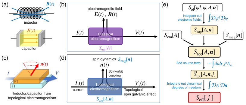
Figure 1: Schematic images of conventional and topological electromagnetism: (a) Illustrations of conventional inductors and capacitors based on classical electromagnetism. The inductance arises from the dynamics of magnetic field $\boldsymbol{B}(t)$, and the capacitance arises from the dynamics of electric field $\boldsymbol{E}(t)$. (b) Theoretical structure of conventional inductors and capacitors, which consists of the Maxwell’s classical electromagnetic action $S_{\mathrm{em}}[A]$. (c) Illustration of an inductor or a capacitor based on topological electromagnetism. As an example, we take a heterostructure of a topological insulator (TI) and a ferromagnetic insulator (FI), and make use of the magnetization dynamics $\boldsymbol{n}(t)$. See Fig. 2(a) for the detailed setup. (d) Theoretical structure of inductors and capacitors based on topological electromagnetism, which consists of the topological magnetoelectric action $S_{\mathrm{top}}[A,\boldsymbol{n}]$ and the action for spin dynamics $S_{\mathrm{mag}}[\boldsymbol{n}]$. (e) Image of our field-theoretical framework to derive inductance and capacitance emerging from topological electromagnetism. Effective action $S_{\mathrm{eff}}[j]$ describing inductance and capacitance for the charge degrees of freedom $j$ can be derived from the topological magnetoelectric action $S_{\mathrm{top}}[A,\boldsymbol{n}]$, which involves the dynamics of electromagnetic fields $A$ and spins (magnetization) $\boldsymbol{n}$.

Topological field theory of electromagnetic fields describes anomalous magnetoelectric responses in materials that cannot be described by the conventional Maxwell’s equations [1, 2, 3, 4, 5, 6, 7]. For instance, the surface state of a three-dimensional (3D) topological insulator (TI) [8, 9] with magnetism shows the intrinsic anomalous Hall effect (AHE) [10, 11, 12] and the universal magneto-optical effects [13, 14, 15], which are described by the $(2+1)$D Chern–Simons theory [16, 17, 18]. The edge state of a 2D quantum spin Hall insulator (QSHI) [19, 20, 21] is capable of the quantized charge pumping [22, 23, 24], which is described by the topological action known as the $\theta$-term in $(1+1)$D [25]. Such anomalous magnetoelectric responses are realized by the electronic states with nontrivial band topology in materials, which we term here as topological electromagnetism. Notably, the topological magnetoelectric responses emerging in insulators are free from energy dissipation by Joule heating. Such nondissipative magnetoelectric responses are capable of designing power-saving electronics and spintronics devices, such as magnetic memories using the topologically induced spin torques [17, 26, 27, 28, 29, 30].

In particular, in a circuit component, the power efficiency is characterized by the quality factor ($Q$-factor),

$$Q_{\omega}=\left|\frac{\mathrm{Im}Z_{\omega}}{\mathrm{Re}Z_{\omega}}\right|.$$ (1)

Here $Z_{\omega}$ is the complex impedance of the circuit component, at the operation frequency $\omega$. To achieve a high $Q$-factor, one needs to reduce the power loss from the resistance $\mathrm{Re}Z_{\omega}$ and to enhance the reactance $\mathrm{Im}Z_{\omega}$. However, inductors and capacitors, which are the most fundamental elements broadly used in electric circuits, are still based on classical electromagnetism [see Figs. 1(a) and (b)] [31]. Inductors use the dynamics of magnetic fields threading magnetic cores in coils, and capacitors use the dynamics of electric fields in dielectric media between metallic plates. Since they operate with conduction currents in metals, power loss by internal resistance is inevitable, which reduces the $Q$-factor.

In this work, we establish a theory of inductors and capacitors based on topological electromagnetism in insulators, by making use of topological electronic systems and spin dynamics [see Fig. 1(c)]. The electrons in topological materials show strong spin-charge coupling due to the band inversion by spin-orbit coupling (SOC) [9, 20, 8, 21]. As a result of the spin-charge coupling, the system significantly shows the dynamical current-voltage response, which can be regarded as an inductance or a capacitance [see Fig. 1(d)]. Moreover, owing to the dissipationless nature of topological electromagnetism, power loss is much suppressed and a high $Q$-factor is achieved, in comparison with conventional inductors and capacitors.

In order to study such inductive and capacitive behaviors in insulators, we build a framework to derive an effective field theory that describes the current-voltage response of the system, which is schematically illustrated in Fig. 1(e). In this framework, we combine topological electromagnetism with the dynamics of spins and electromagnetic fields, and integrate out the microscopic degrees of freedom. As a result, we reach the effective action for the collective dynamics of electric current, which can be directly compared with the classical action for electric circuits [32, 33]. To demonstrate the emergence of an inductance and a capacitance, we take a heterostructure composed of a 3D TI and a ferromagnetic insulator (FI) [34, 35, 36, 37, 38], and apply our framework. We chacaterize the inductance appearing here in comparison with the recently reported “emergent inductance”, which is the inductive behavior caused by spin dynamics in magnetic metals [39, 40, 41, 42, 43, 44], by focusing on their operation frequencies and $Q$-factors. Due to the absence of metallic conduction in TI, the internal resistance $\mathrm{Re}Z_{\omega}$ is largely suppressed in the TI-FI heterostructure, giving rise to a high $Q_{\omega}\approx 10\text{--}100$. Moreover, the inductance of the TI-FI heterostructure is available up to the frequency of the ferromagnetic resonance (FMR) in the FI, which is around $\omega\approx 1\text{--}10\ \mathrm{GHz}$. This is in a clear contrast with the previously reported emergent inductors using magnetic textures [39, 40, 41, 43, 44], whose operation frequencies are limited up to $10\text{--}100\>\mathrm{kHz}$ due to the pinning of magnetic textures. We conclude that TIs are capable of realizing an inductance with a high $Q$-factor in the high frequency regime.

I Results

Theoretical framework. We first show the theoretical framework to treat the contribution of topological electromagnetism to the complex impedance, the process of which is summarized in Fig. 1(e). We formulate the coupled dynamics of the electric current (or the electromagnetic fields) and the magnetization, in the Lagrangian formalism of quantum field theory. We take $\hbar=1$ throughout this article. Classical electromagnetism described by the Maxwell’s action, $\displaystyle S_{\mathrm{em}}[A]$ $\displaystyle=\frac{1}{2}\int dtd\boldsymbol{r}\left[\epsilon|\boldsymbol{E}|^{2}-\mu^{-1}|\boldsymbol{B}|^{2}\right],$ (2) accounts for conventional inductance and capacitance as illustrated in Fig. 1(a). Here $A=(A_{0},\boldsymbol{A})$ is the gauge potential for the electric field $\boldsymbol{E}=-\boldsymbol{\nabla}A_{0}-\partial_{t}\boldsymbol{A}$ and the magnetic field $\boldsymbol{B}=\boldsymbol{\nabla}\times\boldsymbol{A}$, with the dielectric permittivity $\epsilon$ and the magnetic permeability $\mu$.

Topological electromagnetism in materials comes from the coupling between the electromagnetic fields and topological electron systems. Moreover, if the system contains a magnetic ordering, the magnetic moments also participate in topological electromagnetism via the coupling to the electron spins, as illustrated in Fig. 1(d). Here we denote the effect of topological electromagnetism symbolically as the topological action $S_{\mathrm{top}}[A,\boldsymbol{n}]$, where the symbol $\boldsymbol{n}$ charactetizes the magnetic ordering. For the clarity of discussion, here we take a ferromagnet with the magnetization pointing to the direction $\boldsymbol{n}$. Microscopically, $S_{\mathrm{top}}$ can be derived from the action $S_{\mathrm{el}}[\psi^{\dagger},\psi,A,\boldsymbol{n}]$ for the electron system coupled with the electromagnetic fields and the magnetization. By integrating out the fields $(\psi^{\dagger},\psi)$ of the electrons,

$$S_{\mathrm{top}}[A,\boldsymbol{n}] =-i\ln\int\mathcal{D}\psi^{\dagger}\mathcal{D}\psi\ e^{iS_{\mathrm{el}}[\psi^{\dagger},\psi,A,\boldsymbol{n}]},$$ (3)

we obtain the topological action $S_{\mathrm{top}}[A,\boldsymbol{n}]$. The form of $S_{\mathrm{top}}$ depends on the dimensionality and symmetry of the system, which has been thoroughly studied in the context of topological field theory [1, 2].

In addition, the magnetic ordering $\boldsymbol{n}$ is subject to the precessional dynamics of spins, which we symbolically denote by the action $S_{\mathrm{mag}}[\boldsymbol{n}]$. If the fluctuation around the ground-state magnetic ordering is sufficiently small, the dynamics can be described by the bosonic fields of spin-wave excitations (magnons).

Thus, in topological materials, the coupled dynamics of the electromagnetic fields $A$ and the magnetic ordering $\boldsymbol{n}$ is described by the action

$$S_{\mathrm{tot}}[A,\boldsymbol{n}] =S_{\mathrm{em}}[A]+S_{\mathrm{mag}}[\boldsymbol{n}]+S_{\mathrm{top}}[A,\boldsymbol{n}].$$ (4)

From this action $S_{\mathrm{tot}}$, we now explore the collective dynamics of the electrons, namely, the dynamics of electric charge and current. As the field variable conjugate to the electromagnetic field $A$, we introduce 4-vector field $j=(\rho,\boldsymbol{j})$, with the charge density $\rho$ and the current density $\boldsymbol{j}$. By adding the source term,

$$\tilde{S}_{\mathrm{tot}}[A,\boldsymbol{n},j] =S_{\mathrm{tot}}[A,\boldsymbol{n}]-\int dtd\boldsymbol{r}\ j^{\mu}A_{\mu},$$ (5)

and integrating out the dynamical degrees of freedom $(A,\boldsymbol{n})$, we reach the effective action $S_{\mathrm{eff}}[j]$ which describes the dynamics of $\boldsymbol{j}$,

$$S_{\mathrm{eff}}[j] =-i\ln\int\mathcal{D}A\mathcal{D}\boldsymbol{n}\ e^{i\tilde{S}_{\mathrm{tot}}[A,\boldsymbol{n},j]}.$$ (6)

This formal solution is the main result of this work. From this form, we can understand the inductive and capacitive behavior of the system. Up to bilinears in $j$, it can be compared with the Lagrangian forms of a conventional inductor $(L)$ and capacitor $(C)$ [32, 33],

$$S_{L}[I]=\frac{1}{2}L\int dt\ I^{2}(t),\quad S_{C}[I]=-\frac{1}{2C}\int dt\ P^{2}(t),$$ (7)

where $I(t)$ is the current flowing in an inductor of the inductance $L$, and $P(t)=\int dt\ I(t)$ is the electric polarization in a capacitor of the capacitance $C$. By this way, we obtain the comprehensive expression of the impedance, including inductance $L$ and capacitance $C$, which emerge from the interplay of topological electromagnetism and spin dynamics.

Interface of topological insulator and ferromagnetic insulator. As a demonstration of the effect of topological electromagnetism on the impedance, we consider a heterostructure of a 3D TI and a FI as shown in Fig. 2(a) (see Methods for detalis of the calculation process). The Dirac electrons on the TI surface obtain a mass gap once they are coupled to the out-of-plane magnetization of the FI [1, 45]. The topological field theory arising from $(2+1)$D massive Dirac fermions is the Chern–Simons action [16, 17, 18], $\displaystyle S_{\mathrm{top}}[A,\boldsymbol{n}]$ $\displaystyle=\frac{\sigma_{H}}{2}\int dtd^{2}\boldsymbol{r}\ \epsilon^{\mu\nu\lambda}\mathcal{A}_{\mu}\partial_{\nu}\mathcal{A}_{\lambda},$ (8) where $\sigma_{H}=-\frac{e^{2}}{2\pi}\mathrm{sgn}(n_{z})$ is the half-quantized Hall conductivity, with the elemental charge $e(>0)$, and $\epsilon^{\mu\nu\lambda}$ with $\mu,\nu,\lambda=0,x,y$ is the Levi–Civita symbol in $(2+1)$D. Here $\mathcal{A}$ is the gauge field coupling to the Dirac electrons at the interface. Due to the spin-momentum locking structure at the TI-FI interface, the spatial (in-plane) components of $\mathcal{A}$ consist of both the electromagnetic fields $\boldsymbol{A}$ and the magnetization $\boldsymbol{n}$, as $\boldsymbol{\mathcal{A}}=\boldsymbol{A}-\tfrac{J}{ev}\hat{\boldsymbol{z}}\times\boldsymbol{n}$. $J$ parametrizes the interfacial exchange coupling strength betweeen the electron spin and magnetization $\boldsymbol{n}$, and $v$ denotes the Fermi velocity of the Dirac electrons. This Chern–Simons action accounts for the AHE, yielding the Hall current $\boldsymbol{j}=\sigma_{H}\hat{\boldsymbol{z}}\times\boldsymbol{E}$ [10, 11, 12]. Moreover, there are cross terms of $\boldsymbol{A}$ and $\boldsymbol{n}$ in the action $S_{\mathrm{top}}[A,\boldsymbol{n}]$, which can be regarded as the effective coupling mediated by the topological electrons. It is proposed that such an effective coupling leads to the electric charging of magnetic textures [18], and also to the electrically induced dynamics of magnetization, which is known as the topological inverse spin-galvanic effect [17, 26].

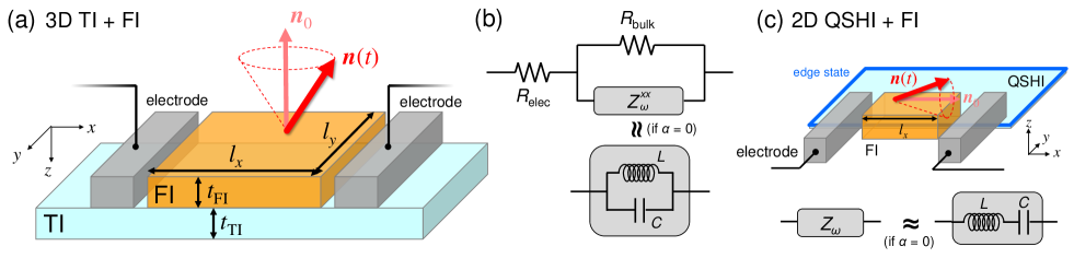
Figure 2: Schematic illustrations for topological inductors and capacitors: (a) The setup using the two-dimensional (2D) interface of a topological insulator (TI) and a ferromagnetic insulator (FI). A current and a voltage are applied longitudinally (in $x$-direction) via the metallic electrodes. The magnetization $\boldsymbol{n}(t)$ in the FI precesses around the ground-state position $\boldsymbol{n}_{0}=-\hat{\boldsymbol{z}}$. The interface is of the length $l_{x}$ and the width $l_{y}$, and the thicknesses of the TI and FI films are defined as $t_{\mathrm{TI}}$ and $t_{\mathrm{FI}}$, respectively. (b) The equivalent circuit for the impedance of the setup (a). In addition to the complex impedance $Z^{xx}_{\omega}$ of the TI-FI interface, we take into account the resistance of the bulk $R_{\mathrm{bulk}}$ and that of the electrodes $R_{\mathrm{elec}}$, and evaluate the total impedance $Z^{\mathrm{tot}}_{\omega}$ given by Eq. (13). In the limit $\alpha=0$, $Z^{xx}_{\omega}$ becomes equivalent to the impedance of a parallel circuit of an inductor $(L)$ and a capacitor $(C)$. (c) The setup using the 1D edge of a quantum spin Hall insulator (QSHI) and a FI. A current and a voltage are applied longitudinally (in $x$-direction) via the metallic electrodes. The magnetization $\boldsymbol{n}(t)$ in the FI precesses around the ground-state position $\boldsymbol{n}_{0}=\hat{\boldsymbol{x}}$. The interface is of the length $l_{x}$, and the volume of the FI film is defined as $V_{\mathrm{FI}}$. In the limit $\alpha=0$, the impedance $Z_{\omega}$ of the interface becomes equivalent to the impedance of a serial circuit of an inductor $(L)$ and a capacitor $(C)$.

The effective action $S_{\mathrm{eff}}[\boldsymbol{j}]$ for the interfacial current $\boldsymbol{j}$ is derived by the field-theoretical framework which we have explained above. For the clarity of the present discussion, we take the ground-state magnetization direction to the out-of-plane direction $\boldsymbol{n}_{0}=-\hat{\boldsymbol{z}}$. By integrating out the dynamical fields $A$ and $\boldsymbol{n}$, we reach the effective action in the bilinear form,

$$S_{\mathrm{eff}}[\boldsymbol{j}] =l_{x}l_{y}\int\frac{d\omega}{2\pi}\frac{z^{\mu\nu}_{\omega}}{2i\omega}j^{\mu}_{-\omega}j^{\nu}_{\omega},\quad(\mu,\nu=x,y)$$ (9)

where $\boldsymbol{j}_{\omega}$ denotes the Fourier component of $\boldsymbol{j}(t)$ of the frequency $\omega$, and $l_{x,y}$ represents the lateral size of the TI-FI interface in each ($x$ or $y$) direction. The tensor $z_{\omega}^{\mu\nu}$ relates the electric field and the current density, $E_{\mu,\omega}=i\omega A_{\mu,\omega}=z_{\omega}^{\mu\nu}j_{\omega}^{\nu}$, which serves as the complex impedance of a unit area at frequency $\omega$. Therefore, the impedance of the interface of the area $l_{x}l_{y}$ is given as $Z_{\omega}^{\mu\nu}=z_{\omega}^{\mu\nu}({l_{\mu}l_{\nu}}/{l_{x}l_{y}})$ (without summation over $\mu,\nu$). Note that the system shows both longitudinal and transverse impedances. In particular, the longitudinal impedance reads

$$Z^{xx}_{\omega} =z_{0}\frac{i\tilde{\omega}}{(1+i\alpha\tilde{\omega})^{2}-\tilde{\omega}^{2}}\frac{l_{x}}{l_{y}t_{\mathrm{FI}}},$$ (10)

where $\tilde{\omega}=\omega/\Omega_{0}$ is the frequency rescaled by the FMR frequency $\Omega_{0}$, and $\alpha$ is the parameter that characterizes the relaxation of magnetization dynamics (Gilbert damping) in the FI. The coefficient $z_{0}\equiv(\mu_{B}/M_{s})\left(J/ev\right)^{2}$, which has the dimension of volume resistivity, is governed by the material parameters of the TI and the FI. $M_{s}$ is the saturation magnetization of the FI, and $\mu_{B}$ is the Bohr magneton. For instance, let us take a heterostructure of $\mathrm{(Bi,Sb)_{2}(Te,Se)_{3}}$ as a TI and yttrium iron garnet (YIG) as a FI thin films. By using the parameters $M_{s}\approx 20\mu_{B}\>\mathrm{nm}^{-3}$ for YIG [46, 47], $J\approx 1\>\mathrm{eV}$ and $v\approx 10^{5}\>\mathrm{m/s}$ for TI-FI interface [48], we obtain $z_{0}\approx 4.5\times 10^{3}\>\mathrm{\mu\Omega}\>\mathrm{cm}$.

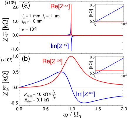
Figure 3: Frequency dependences of the impedance at TI-FI heterostructure: (a) The longitudinal impedance $Z^{xx}_{\omega}$ of the interface given by Eq. (10). We have taken the system size $l_{x}=1\>\mathrm{mm}$, $l_{y}=1\>\mathrm{\mu m}$, $t_{\mathrm{FI}}=10\>\mathrm{nm}$. (b) The impedance of the whole system $Z^{\mathrm{tot}}_{\omega}$ given by Eq. (13), including the bulk resistance $R_{\mathrm{bulk}}=10\>\mathrm{k\Omega}\times(l_{x}/l_{y})$ and $R_{\mathrm{elec}}=0.1\>\mathrm{k\Omega}$. The insets show the magnified views of the impedance at low frequency.

The impedance $Z^{xx}_{\omega}$ shows the resonance structure at $\Omega_{0}$, as shown in Fig. 3(a). Such a resonance structure in the electric circuit comes from the magnetic resonance driven by an AC voltage, which is investigated in Ref. [49]. In the limit $\alpha=0$, the impedance $Z^{xx}_{\omega}$ becomes compatible to that of an $LC$-parallel circuit shown in Fig. 2(b),

$$Z^{xx}_{\omega}\approx\left[\frac{1}{i\omega L}+i\omega C\right]^{-1},$$ (11)

with the inductance and capacitance

$$L=\frac{z_{0}}{\Omega_{0}}\frac{l_{x}}{l_{y}t_{\mathrm{FI}}},\quad C=\frac{1}{z_{0}\Omega_{0}}\frac{l_{y}t_{\mathrm{FI}}}{l_{x}}.$$ (12)

At low frequency up to the FMR frequency $(|\omega|\ll\Omega_{0})$, the impedance shows the inductor-like behavior, $Z^{xx}_{\omega}\approx i\omega L$. The system becomes inductive although the 3D bulk and the 2D interface are insulating, which can be traced back to the 1D conductive edge channels that contribute to the quantum anomalous Hall state. $L$ is proportional to the system length $l_{x}$ and inversely proportional to the cross section $l_{y}t_{\mathrm{FI}}$, which is the common behavior seen in the emergent inductors proposed in previous literature [39, 40, 41, 42, 43, 44]. Thus, they exhibit a large inductance within a small cross section, in contrast to the conventional inductors formed by coils. For the system size $l_{x}=1\>\mathrm{mm},\ l_{y}=1\>\mathrm{\mu m},\ t_{\mathrm{FI}}=10\>\mathrm{nm}$, we can estimate $L=360\>\mathrm{\mu H}$. This $L$ is much larger than the emergent inductances estimated and reported so far using metallic magnets, which is due to the strong spin-momentum locking at the TI-FI interface.

The real part of $Z^{xx}_{\omega}$ for the TI-FI interface becomes proportional to the Gilbert damping constant $\alpha$, $\mathrm{Re}Z^{xx}_{\omega}\approx\alpha\tilde{\omega}^{2}z_{0}(l_{x}/l_{y}t_{\mathrm{FI}})$ for $|\omega|\ll\Omega_{0}$. It implies that the energy dissipation occurs exclusively from the relaxation of magnetization dynamics in the FI. Due to the small damping constant in the FI ($\alpha\approx 10^{-4}\text{--}10^{-3}$), we expect that the power loss in the present system is ideally well suppressed in comparison with the conventional and emergent inductors using metals. The sharp resonance structure seen in Fig. 3(a) accounts for the suppression of power loss.

If the measurement is done at room temperature, the internal resistance $R_{\mathrm{bulk}}$ from the bulk conduction becomes nonnegligible [12, 50, 28, 51], which works in parallel to the impedance $Z^{xx}_{\omega}$ from the interface electrons. Moreover, the resistance $R_{\mathrm{elec}}$ of the metallic electrodes and leads is also present in the experimental measurement, which is serially connected to $Z^{xx}_{\omega}$ and $R_{\mathrm{bulk}}$. Therefore, we now consider an equivalent circuit shown in Fig. 2(b). To quantify the power efficiency in the whole system, we evaluate its impedance,

$$Z^{\mathrm{tot}}_{\omega} =R_{\mathrm{elec}}+\frac{1}{\left(Z^{xx}_{\omega}\right)^{-1}+\left(R_{\mathrm{bulk}}\right)^{-1}},$$ (13)

with the system size defined above. We have taken the approximate values of the bulk resistivity $R_{\mathrm{bulk}}=10\ \mathrm{k\Omega}\times(l_{x}/l_{y})$ seen at room temperature in Bi-based TIs [12, 50, 28, 51], the Gilbert damping constant $\alpha=10^{-3}$ seen in YIG [52], and fixed $R_{\mathrm{elec}}=0.1\>\mathrm{k\Omega}$ in Fig. 3(b). In the low-frequency regime $(|\omega|\ll\Omega_{0})$, the reactance $\mathrm{Im}Z^{\mathrm{tot}}_{\omega}$ rises linearly in $\omega$ like an inductor, whereas the resistance $\mathrm{Re}Z^{\mathrm{tot}}_{\omega}$ is dominated by the electrodes $R_{\mathrm{elec}}$. On the other hand, around the FMR frequency $\omega\approx\Omega_{0}$, the impedance is dominated by the bulk resistance $R_{\mathrm{bulk}}$. Here the reactance component $\mathrm{Im}Z^{\mathrm{tot}}_{\omega}$ gets suppressed and the resonance becomes smeared. Therefore, the TI-FI heterostructure exhibits the inductive behavior up to the FMR frequency $\omega\lesssim\Omega_{0}$.

1D edge of quantum spin Hall insulator. As another example, let us breifly mention the case of a 2D QSHI. A QSHI has spin-helical edge states, which are described as 1D Dirac electrons [19, 20, 21]. We consider the case where these edge states within the length $l_{x}$ are coupled to an FI, as shown in Fig. 2(c). We take the volume of the FI $V_{\mathrm{FI}}$, and its magnetization direction $\boldsymbol{n}$ fluctuating around the ground-state magnetization $\boldsymbol{n}_{0}=\hat{\boldsymbol{x}}$. The Dirac electrons on the edge become gapped and contributes to the $(1+1)$D topological action $\displaystyle S_{\mathrm{top}}[A_{x},\boldsymbol{n}]$ $\displaystyle=-e\int dtdx\frac{\theta}{2\pi}\partial_{t}\mathcal{A}_{x},$ (14) known as the $\theta$-term [22, 25], with $\theta=\arctan(n_{y}/n_{x})\approx n_{y}$ if the fluctuation of $\boldsymbol{n}$ around $x$-axis is small. In a manner similar to the $(2+1)$D case, the gauge field $\mathcal{A}_{x}=A_{x}-\tfrac{J}{ev}n_{z}$ contains both the electromagnetic field and the magnetization, with $J$ the exchange coupling strength and $v$ the velocity of the Dirac electrons on the 1D edge. Based on this topological action, we can evaluate the impedance of this QSHI-FI system (see Supplementary Information for the calculation process). In the limit $\alpha=0$, the effective impedance $Z_{\omega}$ becomes compatible to that of an $LC$-serial circuit as shown in Fig. 2(c), $\displaystyle Z_{\omega}$ $\displaystyle\approx i\omega L+\frac{1}{i\omega C},$ (15) with $\displaystyle C=\frac{e^{2}}{4\pi^{2}N_{s}}\frac{1}{\Omega_{0}},\quad L=\frac{4\pi^{2}N_{s}}{e^{2}}\frac{r^{2}}{\Omega_{0}}.$ (16) Here $N_{s}=V_{\mathrm{FI}}M_{s}/\mu_{B}$ is the number of magnetic moments in the FI, and $r=1+\frac{Jl_{x}}{2\pi vN_{s}}$ is the renormalization factor for the spin Berry phase which arises from the topological magnetoelectric coupling in Eq. (14). In contrast to the $(2+1)$D case, this system behaves like a capacitor at low frequency below the FMR frequency $\Omega_{0}$, and hence the system becomes totally insulating in the limit $\omega=0$. This is reasonable, because the present QSHI-FI heterostructure does not have any conducting edge channel, and the electric current is pumped only by the magnetization dynamics driven at finite frequency.

II Discussion

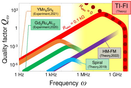
Figure 4: Comparison of the performances of emergent inductors: The operation frequencies $\omega$ and the $Q$-factors $Q_{\omega}$ as functions of $\omega$ are plotted for various emergent inductor setups using magnetization dynamics. The red branches (TI-FI) account for the heterostructure of a topological insulator and a ferromagnetic insulator investigated in this work. The red solid line is our estimation with the internal resistance $R_{\mathrm{elec}}=0.1\>\mathrm{k\Omega}$ of the electrodes, while the dark-red dotted line is the estimation without $R_{\mathrm{elec}}$. The other lines show the theoretically estimated and experimentally measured data of the emergent inductors seen in the previous works (see Discussion section and Supplementary Information for the details and references for the previous works). The TI-FI heterostructure is advantageous in realizing a high $Q$-factor in the yellow-shaded frequency region $(\omega\gtrsim 100\>\mathrm{kHz})$.

Let us now focus on the inductive behavior obtained above. We compare its operation frequency $(\omega)$ and $Q$-factor $(Q_{\omega})$, with those of the emergent inductors using metallic magnets reported in previous literature, which are summarized in Fig. 4. (See Supplementary Information for details of the displayed data.)

In metallic magnets with spin textures, such as magnetic spirals, the interplay of the electric current and the dynamics of the spin textures, known as the spin-transfer torque [53, 54, 55] and the spinmotive force [56, 57, 58], gives rise to the emergent inductance [39, 40, 41]. The emergent inductance was measured in the helimagnetic states of $\mathrm{Gd_{3}Ru_{4}Al_{12}}$ [43] and $\mathrm{YMn_{6}Sn_{6}}$ [44], $L\approx 100\>\mathrm{nH}\text{--}1\>\mathrm{\mu H}$ at frequencies $1\text{--}10\>\mathrm{kHz}$. They show large inductances and high $Q$-factors due to the short helical pitches of a few nanometers. However, the inductances are suppressed at frequencies $\omega\gtrsim 10\>\mathrm{kHz}$. Theoretically, the suppression of emergent inductance is associated to the weakening of extrinsic pinning at high frequency.

In a heterostructure of heavy metal (HM) and ferromagnetic metal (FM), interplay of the current and the magnetization dynamics is governed by SOC, and the emergent inductance arises even if the magnetization is uniform [42]. The operation frequency is not limited by the depinning effect, and it reaches as high as the FMR frequency. In the heterostructure of Co and Pt, the emergent inductance of $L\approx 0.1\>\mathrm{nH}$ is estimated for the area of $1\>\mathrm{\mu m}\times 1\>\mathrm{\mu m}$ and the thickness of $10\mathrm{nm}$, up to the order of $\mathrm{GHz}$. On the other hand, due to the metallicity in the bulk, the inductive behavior accompanies a large conduction current that is unnecessary for the inductive behavior. Such a large operation current leads to the Joule heating by the bulk resistivity, which reduces the $Q$-factor below unity.

In comparison with the emergent inductors listed above, the topological electromagnetism in TIs is advantageous in realizing an emergent inductor with a high operation frequency, a low opeation current, and a high $Q$-factor. Since the emergent inductors with TIs use dynamics of uniform magnetization, the operation frequency can reach the FMR frequency of the order of $1\text{--}10\ \mathrm{GHz}$, which is much higher than those of the spiral magnets. Compared with the HM-FM heterostructures, the bulk conduction that is unnecessary for the emergent inductance is much suppressed in TIs, and hence the emergent inductors using TIs can operate with a lower current and a higher $Q$-factor. These advantages can be understood within the unified framework shown here based on the topological field theory.

While topological field theory has been intensely studied from its geometrical aspects, its practical advantage in describing physical phenomena is not well explored so far. Our theoretical study clearly demonstrates its new practical advantage, in understanding and designing power-efficient inductors and capacitors using topological materials. While we have incorporated the dynamics of ferromagnetic ordering $\boldsymbol{n}(t)$ in Fig. 1(e) to demonstrate our field-theoretical treatment of the inductance and capacitance, $\boldsymbol{n}(t)$ can be replaced with any other types of orderings that couple to electron systems. For instance, recent theoretical and experimental studies have discovered a class of antiferromagnetic insulators, called the axion insulators, whose magnetoelectric responses are described by the topological action known as the $\theta$-term in $(3+1)$D [61, 5, 59, 60]. The dynamics of antiferromagnetic ordering (Néel vector) may give rise to topological inductance and capacitance therein. Moreover, our theoretical framework may not be limited to magnetic orderings, but can also be extended to charge orderings and superconductivity, which is left for future studies.

III Methods

Calculation process at TI-FI interface. The electrons at the TI surface are described by the 2D Dirac Hamiltonian with spin-momentum locking, $\mathcal{H}_{\mathrm{el}}^{0}=v(\boldsymbol{p}\times\boldsymbol{\sigma})_{z}$, where $v$ denotes the Fermi velocity at low energy, $\boldsymbol{p}=-i\boldsymbol{\nabla}$ is the momentum operator, and $\boldsymbol{\sigma}$ is the Pauli matrix representing the electron spin. Here we assume that the bulk of the TI and FI is fully insulating and will not consider the bulk conduction. The surface Dirac electrons are coupled to the electromagnetic fields $A$ by the minimal coupling $-j^{\mu}A_{\mu}$, and to the magnetization $\boldsymbol{n}$ of the FI by the exchange coupling $J\boldsymbol{n}\cdot\boldsymbol{\sigma}$ (with the coupling constant $J>0$). Then the action $S_{\mathrm{el}}[\psi^{\dagger},\psi,A,\boldsymbol{n}]$ reads $\displaystyle S_{\mathrm{el}}[\psi^{\dagger},\psi,A,\boldsymbol{n}]=\int dtd^{2}\boldsymbol{r}\ \psi^{\dagger}\left[\pi_{0}-v(\boldsymbol{\pi}\times\boldsymbol{\sigma})_{z}-Jn_{z}\sigma_{z}\right]\psi,$ (17) where the momentum operators are defined by $\displaystyle\pi_{0}\equiv i\partial_{t}-eA_{0},\quad\boldsymbol{\pi}\equiv\boldsymbol{p}-e\boldsymbol{\mathcal{A}}\equiv-i\boldsymbol{\nabla}-e\left[\boldsymbol{A}-\tfrac{J}{ev}\hat{\boldsymbol{z}}\times\boldsymbol{n}\right].$ Note that the in-plane components of the magnetization $\boldsymbol{n}$ leads to the shift of the momentum and acts like the vector potential. On the other hand, the out-of-plane component $n_{z}$ opens a gap at the Dirac point and leads to the massive Dirac spectrum $E_{\pm}(\boldsymbol{k})=\pm\sqrt{(vk)^{2}+(Jn_{z})^{2}}$. This mass gap gives rise to the momentum-space Berry curvature $\Omega^{\pm}_{z}(\boldsymbol{k})=\mp\frac{Jn_{z}}{2|E_{\pm}(\boldsymbol{k})|^{3}}$ for the eigenstates $E_{\pm}(\boldsymbol{k})$, which is the source of the topological magnetoelectric responses. If the Fermi level lies inside the gap of the massive Dirac spectrum, the whole system, including both the bulk and the interface, becomes insulating. By integrating out the fermionic fields, the topological action $S_{\mathrm{top}}[A,\boldsymbol{n}]$ results in the $(2+1)$D Chern–Simons form shown by Eq. (8).

In addition to $S_{\mathrm{top}}$, we formulate the dynamics of the magnetization $S_{\mathrm{mag}}$ and the electromagnetic fields $S_{\mathrm{em}}$. The fluctuation of magnetization around the ground-state position, $\boldsymbol{u}=\boldsymbol{n}-\boldsymbol{n}_{0}$ (with $\boldsymbol{n}_{0}=-\hat{\boldsymbol{z}}$), is described as magnons. Here we assume that the magnetization is formed by the spins with the magnitude $S_{0}$ for each spin, distributed at the number density $\nu_{s}$. Then the saturation magnetization $M_{s}$ becomes $M_{s}=\nu_{s}\mu_{B}S_{0}$. The spin variable $\boldsymbol{S}(\boldsymbol{r},t)$ is related to $\boldsymbol{n}(\boldsymbol{r},t)$ as $\boldsymbol{S}=-S_{0}\boldsymbol{n}$. By the Holstein–Primakoff transformation, the fluctuation of spin $\boldsymbol{S}(\boldsymbol{r},t)$ around the ground-state position $S_{0}\hat{\boldsymbol{z}}$ is described by the magnonic field $\phi(\boldsymbol{r},t)$, with the relation

$$S_{x}+iS_{y} =\phi\left[2S_{0}-\phi^{*}\phi\right]^{1/2}.$$ (18)

Therefore, $\phi$ is related to $\boldsymbol{u}$ as

$$\phi=-\sqrt{\frac{S_{0}}{2}}\left[u_{x}+iu_{y}+O(S_{0}^{-1})\right].$$ (19)

In terms of $\phi$, the magnetization dynamics is described by the effective action

$$S_{\mathrm{mag}}[\boldsymbol{n}] =\nu_{s}\int_{\mathrm{FI}}dtd^{3}\boldsymbol{r}\ \phi^{*}[i\partial_{t}-\Omega(\boldsymbol{p})]\phi,$$ (20)

where $\Omega(\boldsymbol{p})$ denotes the magnon dispersion as a function of momentum $\boldsymbol{p}$. The integral runs over the volume of the FI. Note that the relaxation of magnetization dynamics is omitted in this action, which shall be restored in the discussion later on.

For the electromagnetic fields, we focus on the dynamics induced by the AC current, and hence we omit the magnetic components and keep the electric components,

$$S_{\mathrm{em}}[\boldsymbol{A}] =\frac{\bar{\epsilon}}{2}\int_{\mathrm{full}}dtd^{3}\boldsymbol{r}\ |\boldsymbol{E}|^{2},$$ (21)

where we take the Coulomb gauge $\boldsymbol{E}(\boldsymbol{r},t)=-\partial_{t}\boldsymbol{A}$. The spatial integral runs over the whole system including both the TI and the FI, with $\bar{\epsilon}$ the dielectric permittivity averaged over the whole system.

From $S_{\mathrm{tot}}=S_{\mathrm{top}}+S_{\mathrm{mag}}+S_{\mathrm{em}}$ defined above, we now evaluate the effective action $S_{\mathrm{eff}}$ for the electric current. Here we take the thin-film geometry for the FI and TI, with their thicknesses $t_{\mathrm{FI}}$ and $t_{\mathrm{TI}}$, respectively, and bring them into contact at the interface with the length $l_{x}$ and the width $l_{y}$, as shown in Fig. 2(a). Over the whole system, we assume the spatial homogeneity of the fields $\boldsymbol{A}$ and $\boldsymbol{n}(=-\hat{\boldsymbol{z}}+\boldsymbol{u})$. By this assumption, the total action $S_{\mathrm{tot}}$ can be rearranged in the matrix form for $\boldsymbol{A}$ and $\boldsymbol{u}$,

$$S_{\mathrm{tot}}[\boldsymbol{A},\boldsymbol{u}] =l_{x}l_{y}\int\frac{d\omega}{2\pi}\begin{pmatrix}A_{\omega}^{*}&u_{\omega}^{*}\end{pmatrix}\hat{K}_{\omega}\begin{pmatrix}A_{\omega}\\ u_{\omega}\end{pmatrix},$$ (22)

with the Fourier components $A_{\omega}\equiv A_{x,\omega}+iA_{y,\omega}$ and $u_{\omega}\equiv u_{x,\omega}+iu_{y,\omega}$ labeled by the frequency $\omega$. The components of the kernel matrix $\hat{K}_{\omega}$ read

$$\hat{K}_{\omega}=\begin{pmatrix}K_{\omega}^{AA}&K_{\omega}^{Au}\\ K_{\omega}^{uA}&K_{\omega}^{uu}\end{pmatrix},$$ (23)

$$K_{\omega}^{AA}=\frac{1}{2}\bar{\epsilon}t_{\mathrm{full}}\omega^{2}+\frac{\sigma_{H}}{2}\omega,\quad K_{\omega}^{Au}=\left(K_{\omega}^{uA}\right)^{*}=i\lambda\frac{\sigma_{H}}{2}\omega,$$

$$K_{\omega}^{uu}=\tfrac{1}{2}t_{\mathrm{FI}}\nu_{s}S_{0}(\omega-\Omega_{0}-i\alpha|\omega|)+\lambda^{2}\frac{\sigma_{H}}{2}\omega,$$ (24)

with $t_{\mathrm{full}}=t_{\mathrm{TI}}+t_{\mathrm{FI}}$. Here $\Omega_{0}\equiv\Omega(\boldsymbol{p}=0)$ is the FMR frequency, and $\lambda\equiv J/ev$ is the material parameter characterizing the effect of exchange coupling at the interface. We have restored the effect of the Gilbert damping $\alpha$, by shifting $\Omega_{0}\rightarrow\Omega_{0}+i\alpha|\omega|$. At the frequency $\omega$ lower than the electrostatic energy scale $\Omega_{\mathrm{el}}={e^{2}}/{4\pi\bar{\epsilon}t_{\mathrm{full}}}$, the dielectric part $\frac{1}{2}\bar{\epsilon}t_{\mathrm{full}}\omega^{2}$ in $K_{\omega}^{AA}$ becomes negligibly small compared to the topological part $(\sigma_{H}/2)\omega$. Since $\Omega_{\mathrm{el}}$ is at the order of $1\>\mathrm{THz}$ in the films of $t_{\mathrm{full}}\approx 10\>\mathrm{nm}$, which is much higher than the FMR frequency, we neglect the dielectric part in the following discussion.

By adding the source term to this action, we have

$$\tilde{S}_{\mathrm{tot}}[\boldsymbol{A},\boldsymbol{u},\boldsymbol{j}]=S_{\mathrm{tot}}[\boldsymbol{A},\boldsymbol{u}]-l_{x}l_{y}\int\frac{d\omega}{2\pi}\boldsymbol{j}_{-\omega}\cdot\boldsymbol{A}_{\omega}$$ (25)

$$=l_{x}l_{y}\int\frac{d\omega}{2\pi}\begin{pmatrix}A_{\omega}^{*}&u_{\omega}^{*}&j_{\omega}^{*}\end{pmatrix}\left(\begin{array}[]{cc|c}K_{\omega}^{AA}&K_{\omega}^{Au}&-\frac{1}{2}\\ K_{\omega}^{uA}&K_{\omega}^{uu}&0\\ \hline\cr-\frac{1}{2}&0&0\end{array}\right)\begin{pmatrix}A_{\omega}\\ u_{\omega}\\ j_{\omega}\end{pmatrix},$$ (29)

with $j_{\omega}=j_{\omega}^{x}+ij_{\omega}^{y}$. By integrating out the dynamical degrees of freedom $A_{\omega}$ and $\phi_{\omega}$, we obtain the effective action for the 2D current density $\boldsymbol{j}$ in the bilinear form,

$$S_{\mathrm{eff}}[\boldsymbol{j}] =l_{x}l_{y}\int\frac{d\omega}{2\pi}\Gamma_{\omega}j_{\omega}^{*}j_{\omega},$$ (30)

with

$$\Gamma_{\omega}=-\frac{1}{4}\left[\hat{K}_{\omega}^{-1}\right]^{AA}=-\frac{1}{4}\frac{K_{\omega}^{uu}}{K_{\omega}^{AA}K_{\omega}^{uu}-K_{\omega}^{Au}K_{\omega}^{uA}}.$$ (31)

By decomposing the real and imaginary parts of $j_{\omega}$, we obtain the form shown by Eq. (9). The longitudinal and transverse parts of the tensor $z_{\omega}^{\mu\nu}\ (\omega\geq 0)$ read

$$z_{\omega}^{xx}=z_{\omega}^{yy} =i\omega\left(\Gamma_{\omega}+\Gamma_{-\omega}\right)$$ (32)

$$=\frac{\lambda^{2}}{t_{\mathrm{FI}}\nu_{s}S_{0}}\frac{i\omega(\Omega_{0}+i\alpha\omega)}{(\Omega_{0}+i\alpha\omega)^{2}-\omega^{2}},$$

$$z_{\omega}^{xy}=-z_{\omega}^{yx} =-\omega\left(\Gamma_{\omega}-\Gamma_{-\omega}\right)$$ (33)

$$=-\frac{1}{\sigma_{H}}-\frac{\lambda^{2}}{t_{\mathrm{FI}}\nu_{s}S_{0}}\frac{\omega^{2}}{(\Omega_{0}+i\alpha\omega)^{2}-\omega^{2}},$$

respectively. The transverse part $z_{\omega}^{xy}$ contains the real constant term $-1/\sigma_{H}$, which comes from the quantized AHE intrinsic to the TI surface. Furthermore, both the longitudinal and transverse parts contain the terms proportional to $\lambda^{2}=(J/ev)^{2}$, which can be regarded as the impedances emerging from the coupling of the TI and the FI. From the above form of $z_{\omega}^{xx}$ given by Eq. (32), we reach $Z^{xx}_{\omega}$ shown in Eq. (10).

Authors contributions

All authors contributed equally to the results presented in this work and the writing of the manuscript.

References

- [1] X.-L. Qi, T. L. Hughes, and S.-C. Zhang, Topological field theory of time-reversal invariant insulators, Phys. Rev. B 78, 195424 (2008).
- [2] S. Ryu, J. E. Moore, and A. W. W. Ludwig, Electromagnetic and gravitational responses and anomalies in topological insulators and superconductors, Phys. Rev. B 85, 045104 (2012).
- [3] A. J. Niemi and G. W. Semenoff, Axial-Anomaly-Induced Fermion Fractionization and Effective Gauge-Theory Actions in Odd-Dimensional Space-Times, Phys. Rev. Lett. 51, 2077 (1983).
- [4] A. N. Redlich, Parity violation and gauge noninvariance of the effective gauge field action in three dimensions, Phys. Rev. D 29, 2366 (1984).
- [5] F. Wilczek, Two applications of axion electrodynamics, Phys. Rev. Lett. 58, 1799 (1987).
- [6] S. C. Zhang, T. H. Hansson, and S. Kivelson, Effective-Field-Theory Model for the Fractional Quantum Hall Effect, Phys. Rev. Lett. 62, 82 (1989).
- [7] A. M. Essin, J. E. Moore, and D. Vanderbilt, Magnetoelectric Polarizability and Axion Electrodynamics in Crystalline Insulators, Phys. Rev. Lett. 102, 146805 (2009).
- [8] L. Fu, C. L. Kane, and E. J. Mele, Topological Insulators in Three Dimensions, Phys. Rev. Lett. 98, 106803 (2007).
- [9] M. Z. Hasan and C. L. Kane, Colloquium: Topological insulators, Rev. Mod. Phys. 82, 3045 (2010).
- [10] K. Nomura and N. Nagaosa, Surface-Quantized Anomalous Hall Current and the Magnetoelectric Effect in Magnetically Disordered Topological Insulators, Phys. Rev. Lett. 106, 166802 (2011).
- [11] R. Yu, W. Zhang, H.-J. Zhang, S.-C. Zhang, X. Dai, and Z. Fang, Quantized Anomalous Hall Effect in Magnetic Topological Insulators, Science 329, 61 (2010).
- [12] C.-Z. Chang, J. Zhang, X. Feng, J. Shen, Z. Zhang, M. Guo, K. Li, Y. Ou, P. Wei, L.-L. Wang, Z.-Q. Ji, Y. Feng, S. Ji, X. Chen, J. Jia, X. Dai, Z. Fang, S.-C. Zhang, K. He, Y. Wang, L. Lu, X.-C. Ma, and Q.-K. Xue, Experimental Observation of the Quantum Anomalous Hall Effect in a Magnetic Topological Insulator, Science 340, 167 (2013).
- [13] W.-K. Tse and A. H. MacDonald, Giant Magneto-Optical Kerr Effect and Universal Faraday Effect in Thin-Film Topological Insulators, Phys. Rev. Lett. 105, 057401 (2010).
- [14] R. Valdés Aguilar, A. V. Stier, W. Liu, L. S. Bilbro, D. K. George, N. Bansal, L. Wu, J. Cerne, A. G. Markelz, S. Oh, and N. P. Armitage, Terahertz Response and Colossal Kerr Rotation from the Surface States of the Topological Insulator , Phys. Rev. Lett. 108, 087403 (2012).
- [15] V. Dziom, A. Shuvaev, A. Pimenov, G. V. Astakhov, C. Ames, K. Bendias, J. Böttcher, G. Tkachov, E. M. Hankiewicz, C. Brüne, H. Buhmann, and L. W. Molenkamp, Observation of the universal magnetoelectric effect in a 3D topological insulator, Nat. Commun. 8, 15197 (2017).
- [16] R. Jackiw, Fractional charge and zero modes for planar systems in a magnetic field, Phys. Rev. D 29, 2375 (1984).
- [17] I. Garate and M. Franz, Inverse Spin-Galvanic Effect in the Interface between a Topological Insulator and a Ferromagnet, Phys. Rev. Lett. 104, 146802 (2010).
- [18] K. Nomura and N. Nagaosa, Electric charging of magnetic textures on the surface of a topological insulator, Phys. Rev. B 82, 161401(R) (2010).
- [19] S. Murakami, N. Nagaosa, and S.-C. Zhang, Spin-Hall Insulator, Phys. Rev. Lett. 93, 156804 (2004).
- [20] C. L. Kane, and E. J. Mele, Quantum Spin Hall Effect in Graphene, Phys. Rev. Lett. 95, 226801 (2005).
- [21] B. A. Bernevig, and S.-C. Zhang, Quantum Spin Hall Effect, Phys. Rev. Lett. 96, 106802 (2006).
- [22] X.-L. Qi, T. L. Hughes, and S.-C. Zhang, Fractional charge and quantized current in the quantum spin Hall state, Nat. Phys. 4, 273 (2008).
- [23] S.-H. Chen, B. K. Nikolić, and C.-R. Chang, Inverse quantum spin Hall effect generated by spin pumping from precessing magnetization into a graphene-based two-dimensional topological insulator, Phys. Rev. B 81, 035428 (2010).
- [24] F. Mahfouzi, B. K. Nikolić, S.-H. Chen, and C.-R. Chang, Microwave-driven ferromagnet–topological-insulator heterostructures: The prospect for giant spin battery effect and quantized charge pump devices, Phys. Rev. B 82, 195440 (2010).
- [25] J. Goldstone and F. Wilczek, Fractional Quantum Numbers on Solitons, Phys. Rev. Lett. 47, 986 (1981).
- [26] T. Yokoyama, J. Zang, and N. Nagaosa, Theoretical study of the dynamics of magnetization on the topological surface, Phys. Rev. B 81, 241410(R) (2010).
- [27] D. Pesin and A. H. MacDonald, Spintronics and pseudospintronics in graphene and topological insulators, Nat. Mater. 11, 409 (2012).
- [28] H. Wu, A. Chen, P. Zhang, H. He, J. Nance, C. Guo, J. Sasaki, T. Shirokura, P. N. Hai, B. Fang, S. A. Razavi, K. Wong, Y. Wen, Y. Ma, G. Yu, G. P. Carman, X. Han, X. Zhang, and K. L. Wang, Magnetic memory driven by topological insulators, Nat. Commun. 12, 6251 (2021).
- [29] Y. Araki and J. Ieda, Intrinsic Torques Emerging from Anomalous Velocity in Magnetic Textures, Phys. Rev. Lett. 127, 277205 (2021).
- [30] M. Yamanouchi, Y. Araki, T. Sakai, T. Uemura, H. Ohta, and J. Ieda, Observation of topological Hall torque exerted on a domain wall in the ferromagnetic oxide , Sci. Adv. 8, eabl6192 (2022).
- [31] J. D. Jackson, Classical Electrodynamics, 3rd Edition (Wiley, New York, 1998).
- [32] D. A. Wells, Application of the Lagrangian Equations to Electrical Circuits, J. Appl. Phys. 9, 312 (1938)
- [33] A. Agarwal and J. Lang, Foundations of Analog and Digital Electronic Circuits (Morgan Kaufmann, Burlington, 2005).
- [34] P. Wei, F. Katmis, B. A. Assaf, H. Steinberg, P. J.-Herrero, D. Heiman, and J. S. Moodera, Exchange-Coupling-Induced Symmetry Breaking in Topological Insulators, Phys. Rev. Lett. 110, 186807 (2013).
- [35] L. D. Alegria, H. Ji, N. Yao, J. J. Clarke, R. J. Cava, and J. R. Petta, Large anomalous Hall effect in ferromagnetic insulator-topological insulator heterostructures, Appl. Phys. Lett. 105, 053512 (2014).
- [36] Z. Jiang, C.-Z. Chang, C. Tang, P. Wei, J. S. Moodera, and J. Shi, Independent Tuning of Electronic Properties and Induced Ferromagnetism in Topological Insulators with Heterostructure Approach, Nano Lett. 15, 5835 (2015).
- [37] C. Tang, C.-Z. Chang, G. Zhao, Y. Liu, Z. Jiang, C.-X. Liu, M. R. McCartney, D. J. Smith, T. Chen, J. S. Moodera, and J. Shi, Above 400-K robust perpendicular ferromagnetic phase in a topological insulator, Sci. Adv. 3, e1700307 (2017).
- [38] K. Yasuda, A. Tsukazaki, R. Yoshimi, K. Kondou, K. S. Takahashi, Y. Otani, M. Kawasaki, and Y. Tokura, Current-Nonlinear Hall Effect and Spin-Orbit Torque Magnetization Switching in a Magnetic Topological Insulator, Phys. Rev. Lett. 119, 137204 (2017).
- [39] N. Nagaosa, Emergent inductor by spiral magnets, Jpn. J. Appl. Phys. 58, 120909 (2019).
- [40] D. Kurebayashi and N. Nagaosa, Electromagnetic response in spiral magnets and emergent inductance, Commun. Phys. 4, 260 (2021).
- [41] J. Ieda and Y. Yamane, Intrinsic and extrinsic tunability of Rashba spin-orbit coupled emergent inductors, Phys. Rev. B 103, L100402 (2021).
- [42] Y. Yamane, S. Fukami, and J. Ieda, Theory of Emergent Inductance with Spin-Orbit Coupling Effects, Phys. Rev. Lett. 128, 147201 (2022).
- [43] T. Yokouchi, F. Kagawa, M. Hirschberger, Y. Otani, N. Nagaosa, and Y. Tokura, Emergent electromagnetic induction in a helical-spin magnet, Nature 586, 232 (2020).
- [44] A. Kitaori, N. Kanazawa, T. Yokouchi, F. Kagawa, N. Nagaosa, and Y. Tokura, Emergent electromagnetic induction beyond room temperature, Proc. Nat. Acad. Sci. 118, e2105422118 (2021).
- [45] X.-L. Qi, Y.-S. Wu, and S.-C. Zhang, Topological quantization of the spin Hall effect in two-dimensional paramagnetic semiconductors, Phys. Rev. B 74, 085308 (2006).
- [46] E. E. Anderson, Molecular Field Model and the Magnetization of YIG, Phys. Rev. 134, A1581 (1964).
- [47] E. J. J. Mallmann, A. S. B. Sombra, J. C. Goes, and P. B. A. Fechine, Yttrium Iron Garnet: Properties and Applications Review, Solid State Phenom. 202, 65 (2013).
- [48] D. Kurebayashi and K. Nomura, Weyl Semimetal Phase in Solid-Solution Narrow-Gap Semiconductors, J. Phys. Soc. Jpn. 83, 063709 (2014).
- [49] J. Tang and R. Cheng, Voltage-Driven Exchange Resonance Achieving 100% Mechanical Efficiency, Phys. Rev. B 106, 054418 (2022).
- [50] Y. Wang, D. Zhu, Y. Wu, Y. Yang, J. Yu, R. Ramaswamy, R. Mishra, S. Shi, M. Elyasi, K.-L. Teo, Y. Wu, and H. Yang, Room temperature magnetization switching in topological insulator-ferromagnet heterostructures by spin-orbit torques, Nat. Commun. 8, 1364 (2017).
- [51] R. Fujimura, R. Yoshimi, M. Mogi, A. Tsukazaki, M. Kawamura, K. S. Takahashi, M. Kawasaki, and Y. Tokura, Current-induced magnetization switching at charge-transferred interface between topological insulator and van der Waals ferromagnet , Appl. Phys. Lett. 119, 032402 (2021).
- [52] M. Haidar, P. Dürrenfeld, M. Ranjbar, M. Balinsky, M. Fazlali, M. Dvornik, R. K. Dumas, S. Khartsev, and J. Åkerman, Controlling Gilbert damping in a YIG film using nonlocal spin currents, Phys. Rev. B 94, 180409(R) (2016).
- [53] J. C. Slonczewski, Conductance and exchange coupling of two ferromagnets separated by a tunneling barrier, Phys. Rev. B 39, 6995 (1989).
- [54] L. Berger, Emission of spin waves by a magnetic multilayer traversed by a current, Phys. Rev. B 54, 9353 (1996).
- [55] Y. Tserkovnyak, A. Brataas, G. E. W. Bauer, and B. I. Halperin, Nonlocal magnetization dynamics in ferromagnetic heterostructures, Rev. Mod. Phys. 77, 1375 (2005).
- [56] L. Berger, Possible existence of a Josephson effect in ferromagnets, Phys. Rev. B 33, 1572 (1986).
- [57] L. Berger, Linear momentum in ferromagnets, J. Phys. C 20, L83 (1987).
- [58] S. E. Barnes and S. Maekawa, Generalization of Faraday’s Law to Include Nonconservative Spin Forces, Phys. Rev. Lett. 98, 246601 (2007).
- [59] R. Li, J. Wang, X.-L. Qi, and S.-C. Zhang, Dynamical axion field in topological magnetic insulators, Nat. Phys. 6, 284 (2010).
- [60] R. S. K. Mong, A. M. Essin, and J. E. Moore, Antiferromagnetic topological insulators, Phys. Rev. B 81, 245209 (2010).
- [61] A. Sekine, and K. Nomura, Axion electrodynamics in topological materials, J. Appl. Phys. 129, 141101 (2021).