Extremal Area of polygons sliding along curves

Abstract.

In this paper we study the area function of polygons, where the vertices are sliding along curves. We give geometric criteria for the critical points and determine also the Hesse matrix at those points. This is the starting point for a Morse-theoretic approach, which includes the relation with the topology of the configuration spaces. Moreover the condition for extremal area gives rise to a new type of billiard: the inner area billiard.

1. Introduction

The study of extremal positions of geometric figures has a long tradition. Well known is the Isoperimetric Problem: Determine the maximal area of a plane figure with given perimeter, see e.g. the historical overview of Blåsjö [Bl].

In this article we focus on polygons, where each vertex slides along its given curve. For triangles this has been studied more than 100 years ago by E. B. Wilson [Wi] , which gave a geometric criterion for a triangle with maximal area.

We consider arbitrary curves, which are (piecewise) $C^{2}$ and develop a general theory for critical polygons of the area function and their Morse theory. In this way we consider all critical polygons and not only maxima and minima. We formulate first results for disjoint curves, but later we also treat intersecting curves and even polygons which have all vertices on a single curve. As long as vertices don’t coincide there is no difference.

First we determine in Theorem 1 the condition for a critical polygon: The tangent line at a vertex is parallel to the (nearest) small diagonal or two neighbouring vertices coincide. Next we compute in Proposition 1 the Hesse matrix at a critical polygon. This matrix depends only on the vertices and on the curvature at the vertices of the critical polygon. We apply this to examples, containing lines or circles.

In section 4 discuss the birth and death of circles originating from a point (considered as a constant curve). We show that generically a critical point in the original setting gives rise to two critical points in the new setting and compare the Morse indices.

In section 5 we discuss polygons, where all vertices are on a single curve. As long no vertices coincide we can use the theory of the first sections. Degenerate polygons (e.g. all vertices coincide) are examples of critical points, which can produces non-isolated singularities. We also discuss the ‘adding of a zig-zag’ and its effect on the Morse indices.

In section 6 we pay attention to the piece-wise differentiable case. Clark subdifferential replaces the usual derivative and tangent cones replace tangent lines. The case of piecewise straight lines (e.g polygons) is an important issue in computational geometry.

In section 7 we give a short introduction to tangential sliding and the conditions for critical area in that case.

We close in section 8 with a proposal for a new billiard: The Inner Area Billiard. The billiard rules follow the conditions for critical points of the (vertex) area function: Every vertex $P_{k+1}$ is constructed by intersecting the boundary curve of the billiard table with the ray from vertex $P_{k-1}$ parallel to the tangent line in vertex $P_{k}$ . This resembles both the usual (perimeter) billiard as the outer (area) billiard. This (as a starting point) rises several billiard type questions.

Note that area functions are affine invariants, so statements stay valid after an affine transformation.

The Morse theoretic approach has been already carried out for the signed area function on linkages with given edge length [KP], [KS1], [KS2], [PZ] and more recently in the context of the isoperimetric problem [KPS]. The case of polygons with vertices on a single ellipse is treated in [Si].

This paper originated from many discussions with Gaiane Panina and George Khimshiasvili during several ‘Research in Residence’ visits at CIRM in Luminy. I wish to thank both and moreover the CIRM and the Mathematical Department of Utrecht University for the good working atmosphere.

2. Vertex Sliding of polygons

2.1. Critical Points

We consider a set of curves $C_{1},\cdots,C_{n}$, embedded in the plane. Each curve is given by a parametrization $C_{i}(t_{i})$.

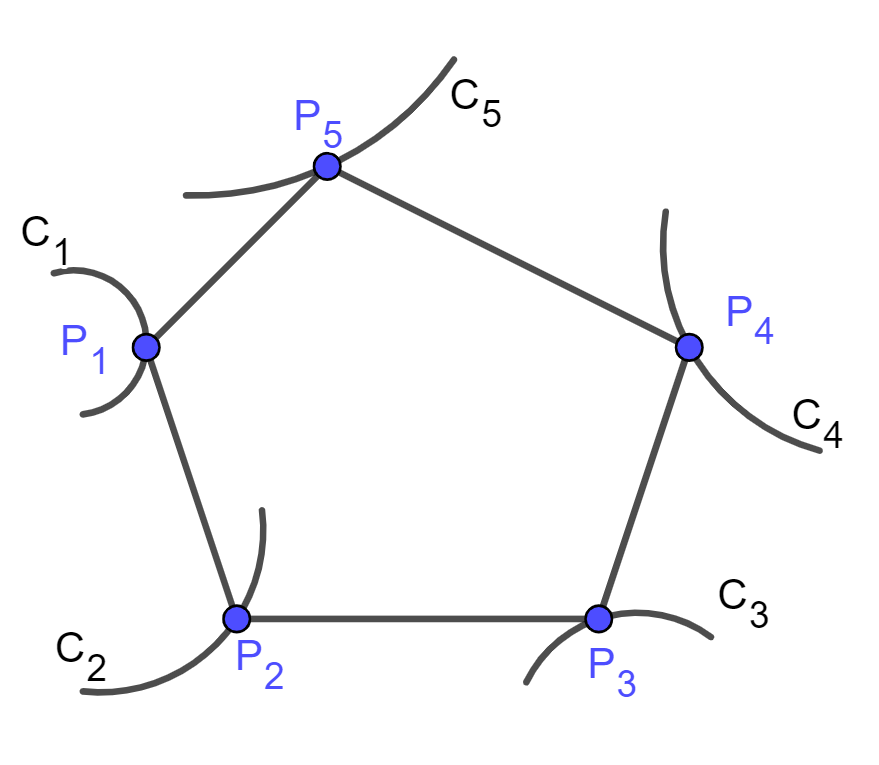
Figure 1. Vertex sliding.

We denote by $C^{{}^{\prime}}_{i}$ the first derivative, by $C^{{}^{\prime\prime}}_{i}$ the second derivative, by $T_{i}$ the unit tangent vector, by $N_{i}$ the unit normal satisfying $T_{i}\times N_{i}=1$ and by $\kappa_{i}$ the curvature. We use the convention that we write indices modulo $n$.

On the product of the source spaces of the curves we define for every set of points $P_{i}=C_{i}(t_{i})$ the signed area function $\mathcal{A}$ as (2-times) the signed area of the polygon $\mathcal{P}$ with vertices $P_{1},\cdots,P_{n}$ (in that order) with coordinates $P_{i}=(x_{i},y_{i})$ by

$$\mathcal{A}=\sum_{i=1}^{n}P_{i}\times P_{i+1}=x_{1}y_{2}-x_{2}y_{1}+\cdots+x_{n}y_{1}-x_{1}y_{n}.$$

We have the following condition for critical points of $\mathcal{A}$:

Theorem 1.

Let $C_{1},\cdots,C_{n}$ be smooth curves in the plane.
$\mathcal{A}$ has a critical point at the polygon $P_{1}\cdots P_{n}$ iff $C_{i}^{{}^{\prime}}\times(C_{i+1}-C_{i-1})=0$ for all $i$ at $(t_{1},\cdots,t_{n}).$ This means:

• $P_{i+1}=P_{i-1}$ or

• $T(P_{i})\parallel P_{i-1}P_{i+1}$

In case of disjoint smooth curves only the parallel conditions apply.

Proof.

$$\mathcal{A}=C_{1}(t_{1})\times C_{2}(t_{2})+C_{2}(t_{2})\times C_{3}(t_{3})+\cdots+C_{n}(t_{n})\times C_{1}(t_{1}).$$

Here $\times$ denote the cross product. The partial derivatives with respect to $t_{i}$ must be 0:

$$C_{i-1}\times C_{i}^{{}^{\prime}}+C_{i}^{{}^{\prime}}\times C_{i+1}=C_{i}^{{}^{\prime}}\times(C_{i+1}-C_{i-1})=0.$$

Since the curves are disjoint and smooth the statement follows. ∎

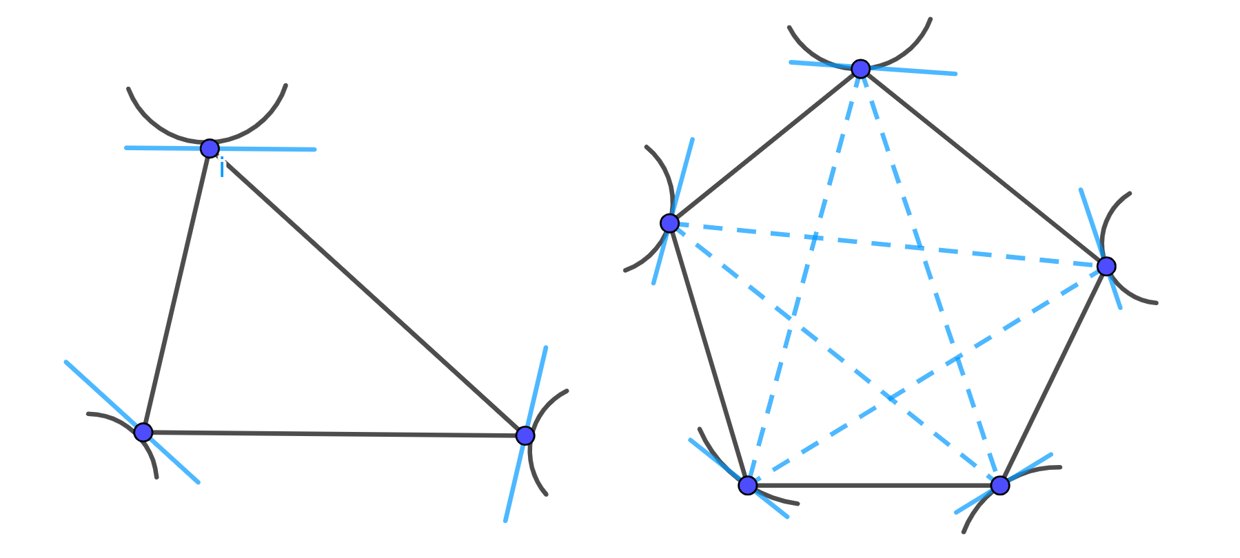
Figure 2. Critical points of $\mathcal{A}$.

Remark 1.

a. If curves $C_{i-1}$ and $C_{i+1}$ intersect, then the intersection point $P_{i-1}=P_{i+1}$ together with the remaining parallel conditions define critical points. When the curves intersect transversally the effect is not significant. If the curves are tangent and $\mathcal{A}$ is critical with $P_{i-1}=P_{i+1}$ then as a consequence the points $P_{i-2},P_{i},P_{i+2}$ must be collinear.

Examples $n=3$: A transversal intersection of two curves will never occur in a critical triangle; unless all 3 curves intersect in that point. But if the two curves are tangent in $P_{1}=P_{3}$ and $P_{2}$ is an intersection point of the tangent line with $C_{2}$ then the ‘triangle’ $P_{1}P_{2}P_{3}$ is a critical point. See Figure 3.

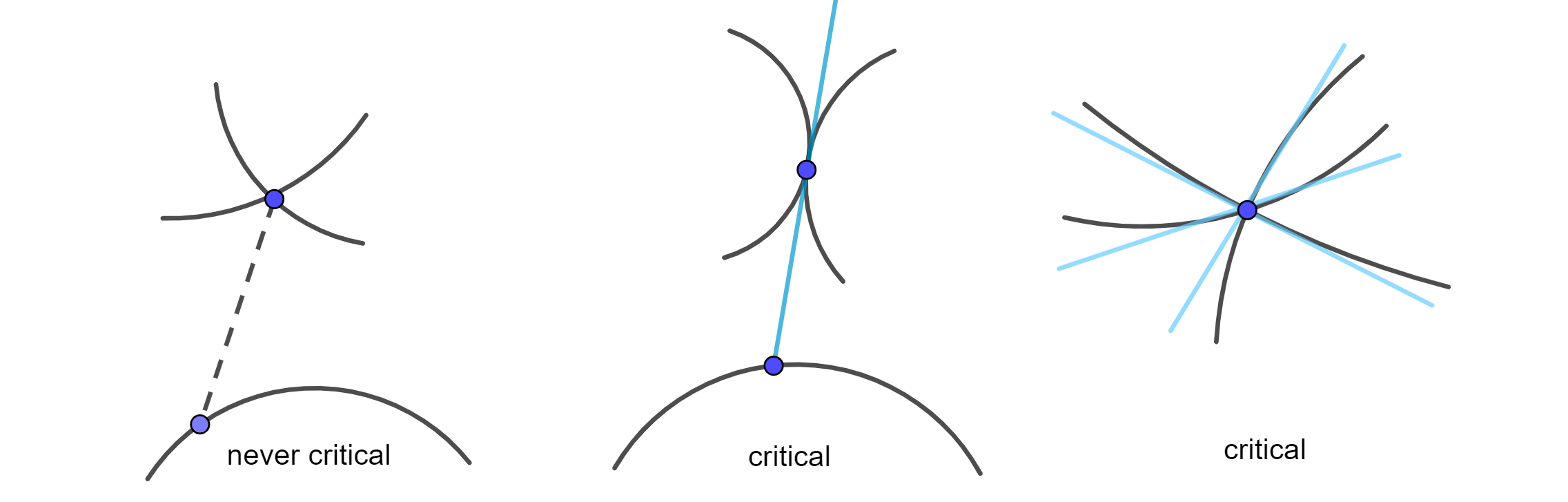
Figure 3. Singular triangles.

b. A special case is: one or more curves coincide. We will meet this in section 5.

c. It is also possible to apply the theorem in cases that one of the curves is a point. We are just left with the other partial derivative conditions. See 4.1 .

2.2. The Hessian

Critical points are determined by first order information about the curves (tangent lines). Next we focus on the second order information.

Proposition 1.

The Hesse matrix of $\mathcal{A}$ is corner tridiagonal

$$H=\begin{pmatrix}a_{1}&b_{1}&0&\cdots&0&b_{n}\\ b_{1}&a_{2}&b_{2}&\cdots&0&0\\ 0&b_{2}&\ a_{3}&\cdots&\cdots&\cdots\\ \dots&\cdots&\cdots&\cdots&\cdots&\dots\\ \cdots&\cdots&\cdots&a_{n-2}&b_{n-2}&0\\ 0&0&\cdots&b_{n-2}&a_{n-1}&b_{n-1}\\ b_{n}&0&\cdots&0&b_{n-1}&a_{n}\\ \end{pmatrix}$$

where $a_{i}=C_{i}^{"}\times(C_{i+1}-C_{i-1})$ and $b_{i}=C_{i}^{{}^{\prime}}\times C_{i+1}^{{}^{\prime}}$.

Note that the matrix elements are $0$ as soon as $|i-j|>1$. Each of the entries are geometric. If we have parametrization via arc length, then

$b_{i}=T_{i}\times T_{i+1}=\sin\alpha_{i}$ and $a_{i}=C^{"}_{i}\times P_{i-1}P_{i+1}=P_{i}M_{i}\times P_{i-1}P_{i+1}$ ,

where $\alpha_{i}=\angle(T_{i},T_{i+1})$ and $M_{i}$ is the center of curvature of $C_{i}$ at the point $P_{i}$. The two vectors in the second product are orthogonal in a critical point. Moreover, if we give the tangent line at $P_{i}$ to $C_{i}$ the same orientation as $P_{1-1}P_{i+1}$ then there is the following sign rule: $a_{i}>0$ if $M_{i}$ is on the left side of the tangent line and $a_{i}<0$ if $M_{i}$ is on the right side. This description does not depend on the orientation of the curve $C_{i}$. Also $a_{i}=\kappa N_{i}\times P_{i-1}P_{i+1}=-\kappa_{i}\epsilon_{i}l_{i}$, where $l_{i}=|C_{i+1}-C_{i-1}|$ and $\epsilon_{i}=+1$ depending on the sign of $a_{i}$.
NB. The sign of $\kappa$ and the vector $N$ depend on the orientation of the curve. If one changes orientation then we get the opposite sign. If we change orientation of one or more curves the Hesse matrix will change by a coordinate transformation of a quadratic form. The sign of the determinant, index and signature will not change.

NB. In section 3.2 we comment on the index of the critical point and how this depends on the positions of the centers of curvature.

NB. A symmetric and tridiagonal matrix (with corners) is quite common in circular systems with neighbouring point interaction.

$\mathcal{A}$ is generically a Morse function. This can already be arranged by translations only:

Proposition 2.

Given $n$ vectors $a_{1},\cdots,a_{n}$, which span the 2-dimensional plane.

• Then $\mathcal{A}$, defined on the translated curves $C_{1}+s_{1}a_{1},\cdots,C_{n}+s_{n}a_{n}$ is Morse for almost every parameter value $s=(s_{1},\cdots,s_{n})$.

• If all curves are compact and $\mathcal{A}$ is Morse for $s=0$ then there is a $\rho>0$ such that $\mathcal{A}$ is also Morse for all $|s|<\rho$.

Proof.

This follows from the stability and parametric transversality theorem ([GP]).

∎

2.3. Higher order approximation

If the critical point is degenerate (non-Morse) the higher order terms become important. We determine here the third order terms in the Taylor series.

We still consider parametrization by arc length and fix notations: If $T$ is the unit tangent vector, then the unit normal vector is defined by $T\times N=1$. In this case $T^{{}^{\prime}}=\kappa N$ and $N^{{}^{\prime}}=-\kappa T$. The terms of order $3$ are:

$$\frac{1}{3!}\big{(}-\sum_{i=1}^{n}\epsilon_{i}l_{i}\dot{\kappa}_{i}\;t_{i}^{3}-3\sum_{i=1}^{n}\kappa_{i}\cos\alpha_{i}\;(t_{i}^{2}t_{i+1}-t_{i}t_{i+1}^{2})\big{)}$$

This follows from the computation of the 3rd order derivatives:

$$a_{iii}=C_{i}^{{}^{\prime\prime\prime}}\times(C_{i+1}-C_{i-1})=(\dot{\kappa}_{i}N_{i}-\kappa_{i}^{2}T_{i})\times\epsilon_{i}l_{i}T_{i}=-\epsilon_{i}l_{i}\dot{\kappa}_{i}$$

$$a_{i+1ii}=C_{i}^{{}^{\prime\prime}}\times C_{i+1}^{{}^{\prime}}=\kappa_{i}N_{i}\times T_{i+1}=-\kappa_{i}\cos\alpha_{i}$$

$$a_{i+1i+1i}=C_{i}^{{}^{\prime}}\times C_{i+1}^{{}^{\prime\prime}}=\kappa_{i}T_{i}\times N_{i+1}=-\kappa_{i}\cos\alpha_{i}$$

$$a_{ijk}=0\;\;\mbox{\rm in all other cases}$$

3. Special cases of vertex sliding

In this section we present several cases, where the curves are lines or circles.

3.1. Sliding along straight lines

The extremal point conditions for $\mathcal{A}$ depend only on the tangent lines. It turns out that the study of lines is an important ingredient in the understanding of more general curves. We first consider the case of 3 lines (with has a surprizing nice answer).

Proposition 3.

In the case of three lines (not through one point) there are global coordinates such that the area function is given by

$$\mathcal{A}=3(t_{1}t_{2}+t_{2}t_{3}+t_{3}t_{1}+\tfrac{1}{4})\mathcal{A}(B_{1}B_{2}B_{3}).$$

where $B_{1}B_{2}B_{3}$ is the triangle formed by the intersection points of the lines. $\mathcal{A}$ has exactly one critical point, which is Morse and has index 2.

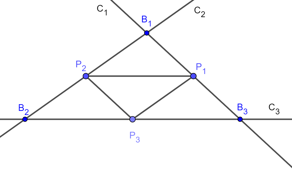
Figure 4. Three lines.

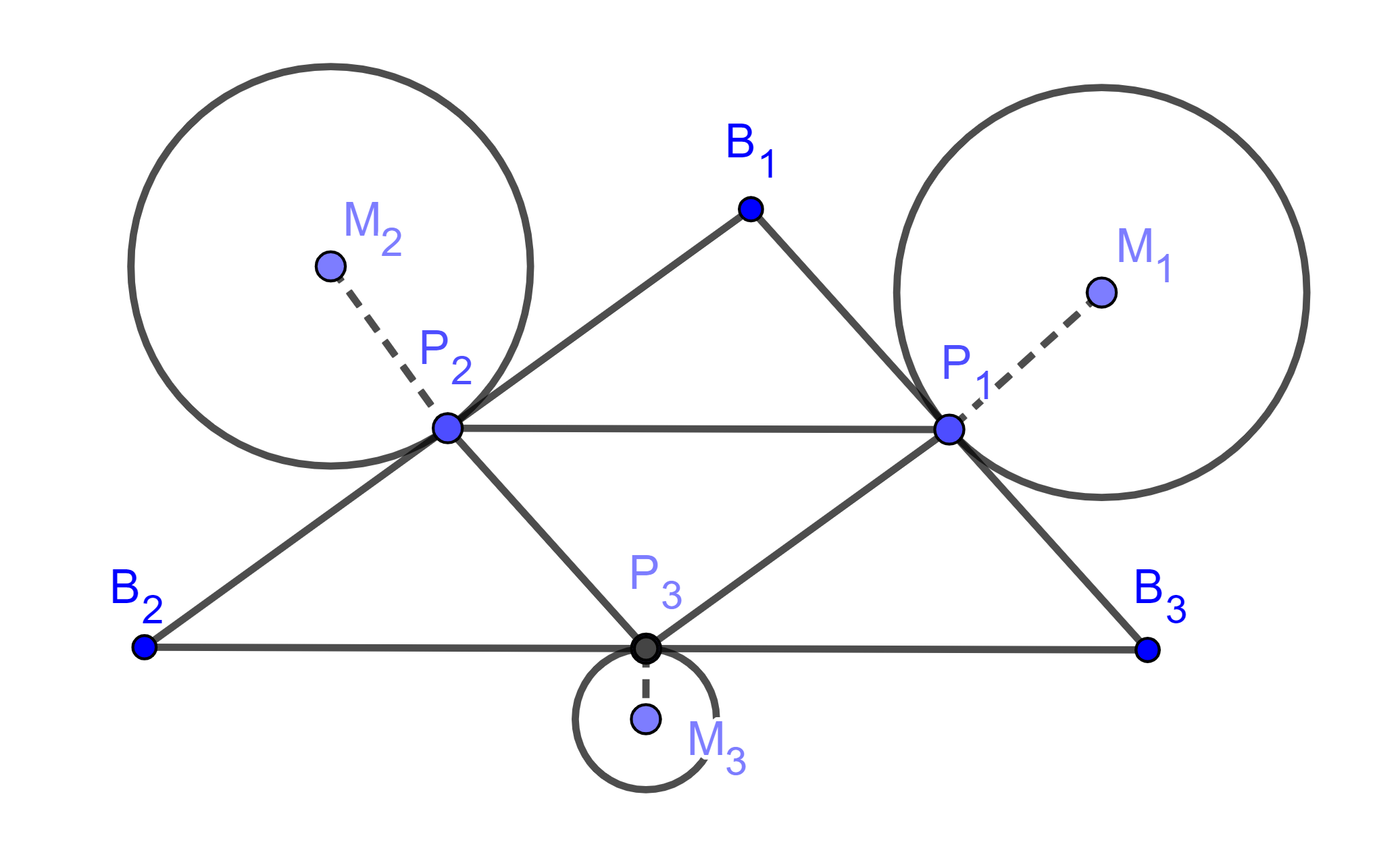
Figure 5. Three circles.

Proof.

Let $C_{i}$ and $C_{i+1}$ intersect in $B_{i}$. Use parametrization $C_{i}(t_{i})=t_{i}B_{i-1}+(1-t_{i})B_{i}$ and perform the computation. After a translation in the coordinates one gets the formula in the theorem. ∎

Remark 2.

In case of 4 lines the parallel conditions imply that opposite sides a parallel (and enclose a parallelogram). In that case there are even infinitely many solutions (non-isolated singular 4-gons). The study of $n$ lines has its own interest, which will be discussed in a future paper.

3.2. Sliding along circles; Hessian and centers of curvature

The critical points and their Hesse matrices depend only on the 2-jets of the curves. For the local study of critical points we can therefore replace the curves by circles, centered in the center of curvature and with radius equal to the radius of curvature.

3.2.1. Three circles in arbitrary position

We consider the case of 3 circles with different radii $r_{i}$ and centers $M_{i}$. If $\mathcal{A}$ is critical then the 3 tangent lines at the vertices of the sliding triangle are parallel to the opposite side of the triangle (see Figure 5). Use clockwise orientation of the circles and their tangent lines .

Proposition 4.

There exists coordinates such that the Hesse matrix at a critical point of $\mathcal{A}$ is:

(1) $$\begin{pmatrix}-m_{1}&s&s\\ s&-m_{2}&s\\ s&s&-m_{3}\\ \end{pmatrix}$$

where $l_{i}$ is the length of the $i^{th}$ edge of the triangle $P_{1}P_{2}P_{s}$ , $m_{i}=\kappa_{i}\epsilon_{i}l_{i}^{3}$ and $s=\frac{1}{2}\mathcal{A}(B_{1},B_{2},B_{3})$.

Proof.

Use parametrization such that $||C_{i}^{{}^{\prime}}(t_{i})||=l_{i}$ . Next insert this in the Hesse matrix in Proposition 1. ∎

The determinant of this matrix is:

(2) $$-m_{1}m_{2}m_{3}+(m_{1}+m_{2}+m_{3})s^{2}+2s^{3}$$

and the eigenvalue equation is:

(3) $$-(\lambda+m_{1})(\lambda+m_{2})(\lambda+m_{3})+(3\lambda+m_{1}+m_{2}+m_{3})s^{2}+2s^{3}=0$$

Discussion: The index of the Hessian depends on a relation between all three radii of curvature. The Hesse matrix is determined by the positions of the 6 points; namely $P_{1},P_{2},P_{3}$ and the centers of curvatures $M_{1},M_{2},M_{3}$. A question is: Is there a geometric criterion in terms of these points, which gives the index or tells when the critical point is non-Morse ? Other questions are: What happens for big and small radii? What if the 3 points lie on the inscribed circle of the triangle defined by the tangent lines ?

The above matrix and formula for the determinant imply already some corollaries:

• If all $|m_{i}|>>0$ then the term $-m_{1}m_{2}m_{3}$ is dominant in the Hessian determinant: So for circles with very small radius this has de effect on the eigenvalues. They are determined by the signs of $\kappa_{i}$.

• If all $m_{i}=0$ then we have saddles (see the section on 3 lines); and this is still the case for very small values of the curvature.

3.2.2. Bifurcations

What can be said about the bifurcation theory for three arbitrary circles ?

We start with a triangle $P_{1}P_{2}P_{3}$. We will use the parallels $P_{i-1}P_{i+1}$ through $P_{i}$ as future tangent line to the circles. The centers $M_{1},M_{2},M_{3}$ are situated at distances $r_{i}$ on the perpendiculars at $P_{i}$ to these lines. We consider the three circles $(M_{i},r_{i})$. They are indeed tangent to the mentioned lines. Note that for all values of $r_{i}$ the polygon $P_{1}P_{2}P_{3}$ is a critical polygon.

Consider as first example the following 1-parameter family of circles: Fix $r_{1}$ and $r_{2}$ and let $r_{3}$ vary. The vanishing of the Hessian determinant (4) gives us (under the condition $m_{1}m_{2}\neq s^{2}$) exactly one bifurcation value $m_{3}^{b}$ for $m_{3}$. To be more precise:

$$m_{3}=\frac{m_{1}s^{2}+m_{2}s^{2}+2s^{3}}{m_{1}m_{2}-s^{2}}$$

For this value $m_{3}^{b}$ the Hessian determinant (evaluated for the polygon $\mathcal{P}=P_{1}P_{2}P_{3}$ changes sign. What happens? A computation with the 3-jet of $\mathcal{A}$ shows, that after a coordinate transform we get the family: $-m_{1}x^{2}-m_{2}y^{2}+\omega z^{2}+z^{3}$, where $\omega$ measures the (signed) difference $m_{3}-m_{3}^{b}$. This means, that $\mathcal{A}$ has a critical point of type $A_{2}$ for that value. In the family a second critical polygon meets our critical polygon at the bifurcation value and moves away after that, while both change to the opposite index.

Next we consider the family where $m_{1}=m_{2}=m_{3}=m$. In that case formula (4) for the Hessian determinant becomes:

(4) $$-m^{3}+3ms^{2}+2s^{3}$$

This happens e.g. when in the above description $\mathcal{P}$ is equilateral and all radii equal: $r_{1}=r_{2}=r_{3}=r$. The Hessian determinant is zero in 2 cases:

$$m=2s\;,\;m=-s\mbox{\rm(double root)}$$

At these two bifurcation values, the first corresponds to the case that all three circles coincide with the inscribed circle of the triangle and $\mathcal{A}$ has a non-isolated singularity (of type $A_{\infty}$). The second to a singularity of corank 2 (type $D$).
The eigenvalue equation becomes:

$$-(\lambda+m-2s)(\lambda+m+s^{2}=0$$

This determines all the Morse indices of $\mathcal{A}$ at the critical polygon $\mathcal{P}$.

3.2.3. Four circles in arbitrary position

We consider the case of 4 circles with different radii $r_{i}$ and centers $M_{i}$. If $\mathcal{A}$ is critical we have that the tangent lines at the vertices of the sliding 4-gon are parallel in pairs to the two diagonals of the quadrilateral. Consider such a situation (see Figure 6).

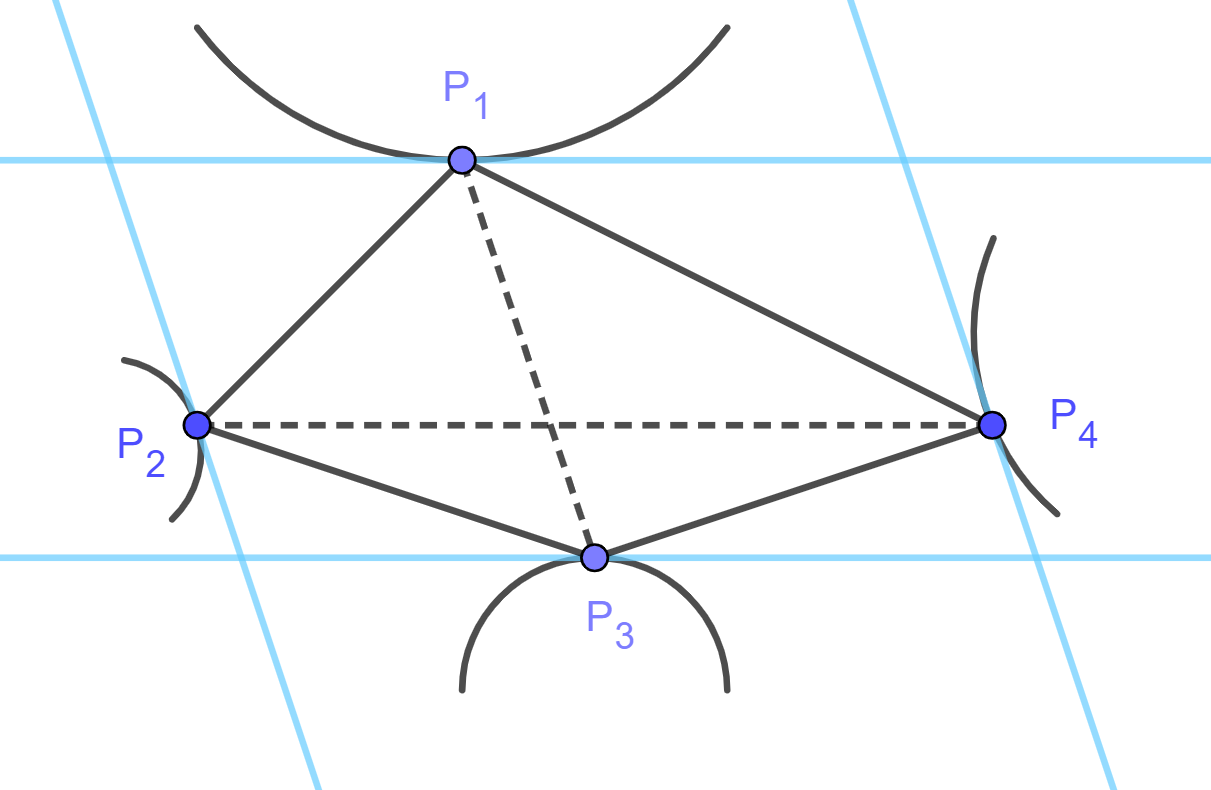
Figure 6. Critical with 4 curves.

Proposition 5.

There exists coordinates such that the Hesse matrix is:

$$\begin{pmatrix}-m_{1}&s&0&s\\ s&-m_{2}&s&0\\ 0&s&-m_{3}&s\\ s&0&s&-m_{4}\\ \end{pmatrix}$$

where $m_{i}=-\kappa_{i}\|P_{i-1}P_{i+1}\|$ and $s=\sin\alpha_{i,i+1}$ where $\alpha_{i,i+1}=\angle(T_{i},T_{i+1}).$

Proof.

Use parametrization of the circles (or curves) by arc length. It is clear that $\alpha_{12}=\alpha_{34}=\pi-\alpha_{23}=\pi-\alpha_{41}$. Next insert this in the matrix of Proposition 1 . ∎

The determinant of this matrix is

$$m_{1}m_{2}m_{3}m_{4}-(m_{1}m_{2}+m_{2}m_{3}+m_{3}m_{4}+m_{4}m_{1})s^{2}$$

For the eigenvalues: replace $m_{i}$ by $\lambda+m_{i}$.
Specializing to all $m_{i}$ are equal we get the eigenvalue equation

$$(m+\lambda)^{2}(m+\lambda-2s)(m+\lambda+2s)=0$$

3.3. Computations with circles

Let $M_{1},\cdots,M_{n}$ be the centers of the circles and $r_{i}$ the corresponding radii. A point $P_{i}$ on circle $C_{i}$ is given by $OM_{i}+r_{i}(\cos\alpha_{i},\sin\alpha_{i})$ and

$$\mathcal{A}=\sum_{i=1}^{n}(OM_{i}+r_{i}(\cos\alpha_{i},\sin\alpha_{i}))\times(OM_{i+1}+r_{i+1}(\cos\alpha_{i+1},\sin\alpha_{i+1})).$$

The usual questions are now: Determine all critical points and their index and to test this with the topology of the n-torus. Is $\mathcal{A}$ a perfect Morse function ? Because of the complexity of the computation it was not possible to find solutions in the general case. This seems also to be the case if we use Lagrange multipliers. In certain explicit examples with fixed parameter one can use computer algebra systems for solving.

We look now next to some special cases, where we try to say more.

3.4. Concentric circles

After choosing the common center M as origin we can use vector notation. A point $P_{i}$ on $C_{i}$ determines the vector $p_{i}$. In this case the criterion for critical point reads as follows: The vector $p_{i}$ is orthogonal to $p_{i+1}-p_{i-1}$ and this is equivalent to the equality of inner products

$$p_{1}\cdot p_{2}=p_{2}\cdot p_{3}=\cdots=p_{n}\cdot p_{1}$$

This gives an equivalent trigonometric criterion in terms of angle-coordinates with the radii as parameters.
The geometric criterion gives in low dimensional cases: (Figure 7)
n=3: The center O is the orthocenter of the triangle $P_{1}P_{2}P_{3}$,
n=4: The two diagonals are orthogonal and intersect in the center O.

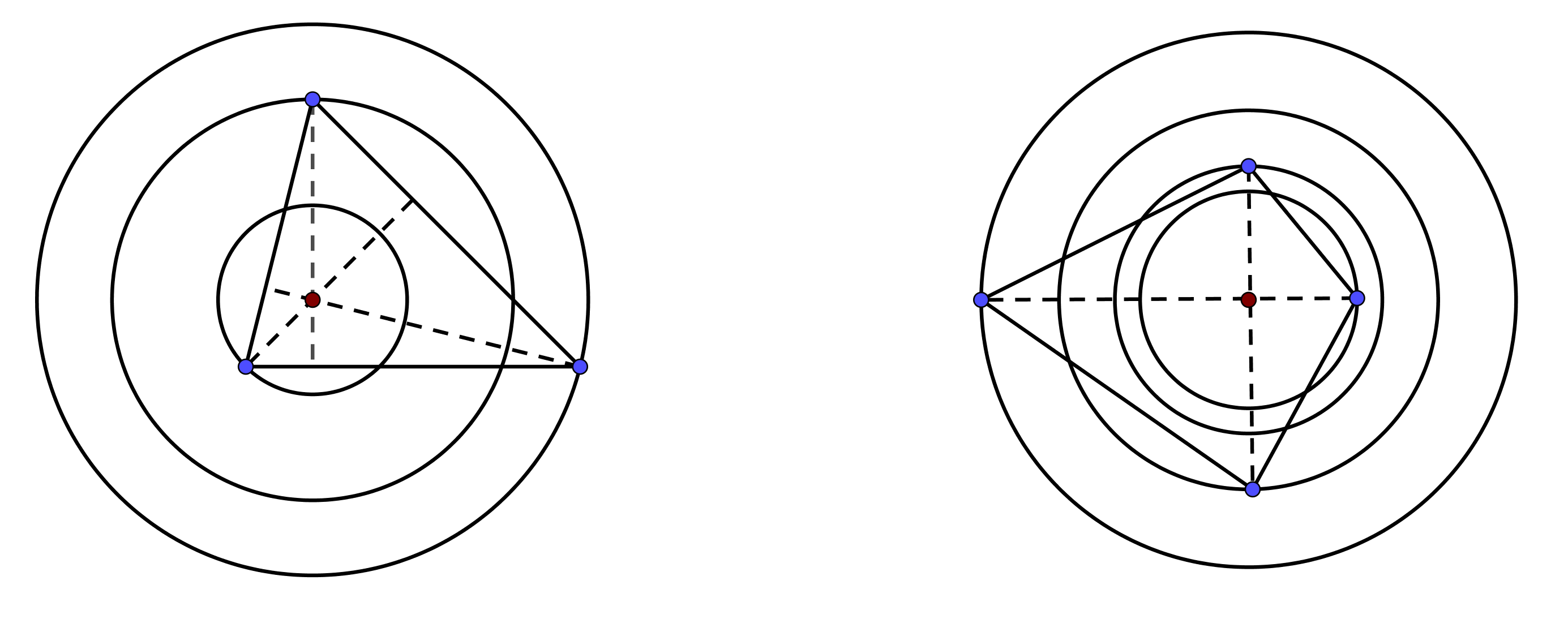
Figure 7. Geometric criterion concentric circles.

In the case of concentric circles we have a rotation symmetry. We will use the reduced configuration space $(S^{1})^{n-1}$. In the (full) configuration space the critical points will appear as product with a circle. The same reduced configuration space occurs as configuration space of $n-1$ concentric circles and a point.

3.4.1. Three concentric circles

Proposition 6.

For 3 concentric circles (with not all radii equal) the area function $\mathcal{A}$ is a perfect Morse function, i.e. has 4 non-degenerate critical points (1 maximum, 2 saddles and 1 minimum).

Proof.

The paper [KS2] studied open n-arms, including a criterion for the critical points of the area function. In the case of 3-arm there is the following relation between the area of arms and the area of a triangle with 3 points on concentric circles:

$$\mathcal{A}(a_{1},a_{2},a_{3})=-\mathcal{A}_{arm}(a_{1},-a_{2},a_{3})$$

As a corollary: The two critical point theories (for 3-arms and for 3 concentric circles) are equivalent. Proposition 6 follows now Theorem 2.1 from [KS2], more especially from the detailed computation in [KS1]. ∎

NB. The criterion for critical 3-arm is (cf Theorem 1.1 of [KS2]) the diacyclic situation (all vertices of the arm are on a circle and the center of the circle is the midpoint of the endpoint vector of the arm; while in the other case the origin of the vectors is equal to the orthocenter of the triangle spanned by the endpoints of the 3 vectors. See Figure 8.

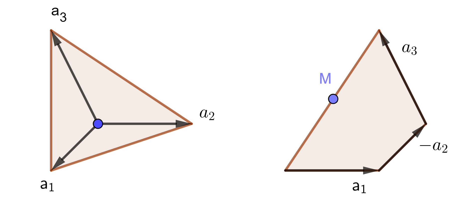
Figure 8. Concentric circles versus Arms.

3.4.2. Four concentric circles

The general criterion for critical point specializes to:
A 4-gon with vertices on 4 concentric circles has a critical point if and only if the diagonals are orthogonal and intersect in the center O.

Proposition 7.

In case of four concentric circles with $r_{1}\neq r_{3}$ and $r_{2}\neq r_{4}$:

• $\mathcal{A}$ has precisely 8 critical points on the 3-torus

• all critical points are Morse.

As a consequence: $\mathcal{A}$ is a perfect Morse function.

Proof.

Consider the following construction:
Start with at any point $P_{1}$ on $C_{1}$. Take a line $l$ from that point to the center. This line has 2 intersection points $P_{3}^{\pm}$ with $C_{3}$. Take next a line through the center orthogonal to $l$ and intersect with $C_{2}$ and $C_{4}$. Altogether we have 8 possibilities $P_{1}P_{2}^{\pm}P_{3}^{\pm}P^{\pm}_{4}$ Compare the right hand side of Figure 7.

Next we compute the Hesse matrix in the critical points by using the formula in (3.3). We fix $\alpha_{1}=0$. Critical points now occur when $\alpha_{2}=\pm\frac{\pi}{2},\alpha_{3}=0$ or $\pi,\alpha_{4}=\pm\frac{\pi}{2}$. The Hesse matrix is as follows:

$$\begin{pmatrix}r_{4}r_{1}-r_{1}r_{2}&-r_{1}r_{2}&0\\ -r_{1}r_{2}&-r_{1}r_{2}+r_{2}r_{3}&r_{2}r_{3}\\ 0&r_{2}r_{3}&-r_{4}r_{3}+r_{2}r_{3}\\ \end{pmatrix}$$

We allow also negative values of the radii, in that way we can deal with all the 8 stationary polygons together. We require $r_{1}>0$. The Hessian determinant is:

$$-r_{1}r_{2}r_{3}r_{4}(r_{4}-r_{2})(r_{3}-r_{1})$$

It follows that as soon as the determinant is non-zero we have 8 critical points which are all of Morse type.

∎

4. Birth and death

4.1. About point-like curves

It is also possible to apply theorem 1 in cases that some of the curves are points. We are just left with the partial derivative conditions for the remaining curves.

Let $C_{i}=P_{i}$ (constant). The effect on the Hesse matrix is that the entries $b_{i-1},a_{i},b_{i}$ become all $0$. If we omit the constant variable $t_{i}$ the reduced matrix becomes ’tridiagonal without corners’ (after the shift in numbering $i\to n$). The seize of the Hesse matrix is reduced by the number of the point-like curves.

$$\begin{pmatrix}a_{1}&b_{1}&0&0&0&b_{6}\\ b_{1}&a_{2}&0&0&0&0\\ 0&0&0&0&0&0\\ 0&0&0&a_{4}&b_{4}&0\\ 0&0&0&b_{4}&a_{5}&b_{5}\\ b_{6}&0&0&0&b_{5}&a_{6}\end{pmatrix}\;\;;\;\;\begin{pmatrix}a_{1}&b_{1}&0&0&b_{6}\\ b_{1}&a_{2}&0&0&0\\ 0&0&a_{4}&b_{4}&0\\ 0&0&b_{4}&a_{5}&b_{5}\\ b_{6}&0&0&b_{5}&a_{6}\end{pmatrix}$$

In case of two or more (pairwise) non-neighbouring points the polygon splits into sub chains with fixed endpoints. The conditions separate the variables over the chains. The Hesse matrix becomes a block matrix with tri-diagonal blocks.

We mention the following sign change rule for the index:

Sylvester Rule: Let $H$ be a symmetric matrix of size $n$. Let $H_{k}$ denotes the $k\times k$ submatrix consisting of the first $k$ rows and columns. We consider the sequence:

(5) $$1,\det H_{1},\det H_{2},\cdots,\det H_{n-1},\det H_{n}.$$

Under the assumption that $H_{k}$ is non-singular for all $k$ the index of the symmetric matrix $H$ is equal to the number of sign changes in the sequence.

We copied this statement form the paper [SV]. It is in fact a consequence of the Jacobi-Sylvester signature rule. We refer to [GR], which contains a historical description.

Remark 3.

What to do if some $\det H_{k}=0$ for some $k<n$ ? We will use that for a non-degenerate matrix the index does not change under small perturbations. Let $H[\epsilon]=H+\epsilon I$. For a proper choice of $\epsilon$ this will not change the index of $H$ and also not of those $H_{k}$ where $\det H_{k}\neq 0$. We can now compute the index of $H$ by counting the sign changes of $\det H[\epsilon]_{k}$. This argument (supplied by Van der Kallen) will be useful at several places in this paper.

4.2. The birth of tangential circles

If we have some constant curves, let small circles grow at those points with well-chosen tangent directions and consider the effect. Compare the left part of Fig 9.

Proposition 8.

Let a subset of the curves $C_{1},\cdots,C_{n}$ be constant (point curves). Consider a critical polygon $\mathcal{P}$. Replace some (or all) point-curves $P_{i}$ by circles, such that the tangent line in $P_{i}$ is parallel to $P_{i-1}P_{i+1}$. Then $\mathcal{P}$ is also a critical polygon for the updated set of curves.
If $\mathcal{P}$ is Morse for the original curves, then for small enough radii, $\mathcal{A}$ is also Morse for the updated curves. The Morse index increases with $0$ or $1$ for each new circle, depending on position of the circle with respect to the tangent line.

Proof.

Consider the small diagonals of the critical polygon $\mathcal{P}$ . Their directions determine also the tangent directions for a critical point is the updated problem. As soon if we replace a constant curve $P_{i}$ by a curve through $P_{i}$ with tangent direction parallel to $P_{i-1}P_{i+1}$ we satisfy the parallel conditions for the updated curves. For the Morse theory: Consider the Hesse matrix in Proposition 1. The original problem corresponds to a submatrix where the $i^{th}$ rows and columns have been deleted for every born circle. (Note that we use here the remark that the second derivative with respect to $t_{i-1}t_{i+1}$ is $0$). It’s determinant is by assumption non-zero.

We intend to use Sylvester’s rule for the statement about indices. We assume $i=n$. Let $C_{n}[r]=O[r]+r(\cos t_{n},\sin t_{n})$ be the circle with radius $r\neq 0$, which is tangent at $P_{n}$ to the line through $P_{n}$, which is paralel to $P_{n-1}P_{1}$. We allow $r<0$ in order to describe circles at both sides of this line. Note that:
$C_{n}[r]^{{}^{\prime}}=r(\sin t_{n},\cos t_{n})$ and $C_{n}[r]^{{}^{\prime\prime}}=-r(\cos t_{n},\sin t_{n})$. Consider next the Hesse matrix $H[r]$, with the entries: $a_{n}[r]=ra_{n}\;,\;b_{n}[r]=rb_{n}\;,\>b_{n-1}[r]=rb_{n-1}$ where $a_{n},b_{n},b_{n-1}$ are the values for $r=1$. All the other $a_{i},b_{i}$ do not depend on $r$. An elementary determinant computation shows:

(6) $$\det H[r]=ra_{n}\det H_{n-1}+r^{2}K\;\;;\;\;(\mbox{ K \rm{ a constant}})$$

Use now Sylvester’s rule. We have the assumption $\det H_{n-1}\neq 0$. It follows that for $|r|\neq 0$ small enough $\det H[r]\neq 0$ and the sign change between the determinants is determined by the sign of $ra_{n}$. This increases the Morse index with 0 or 1.
This reasoning can be repeated for the other point curves. ∎

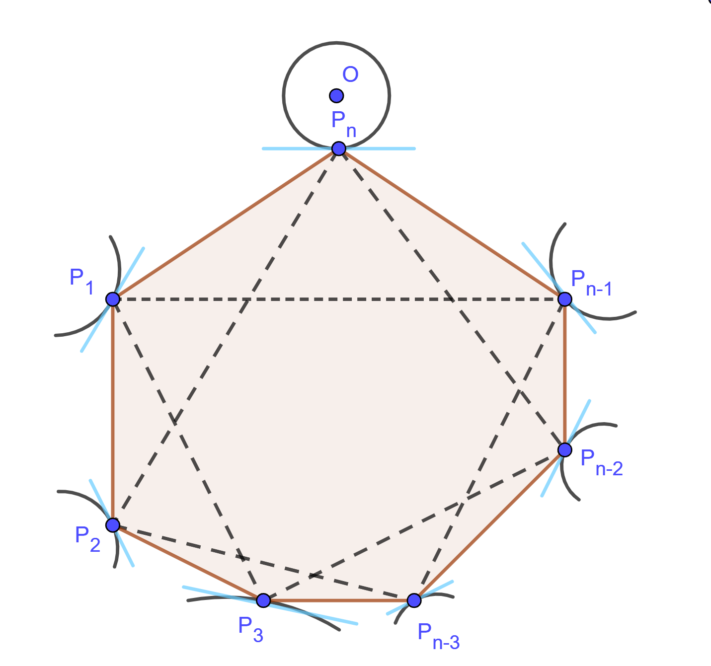
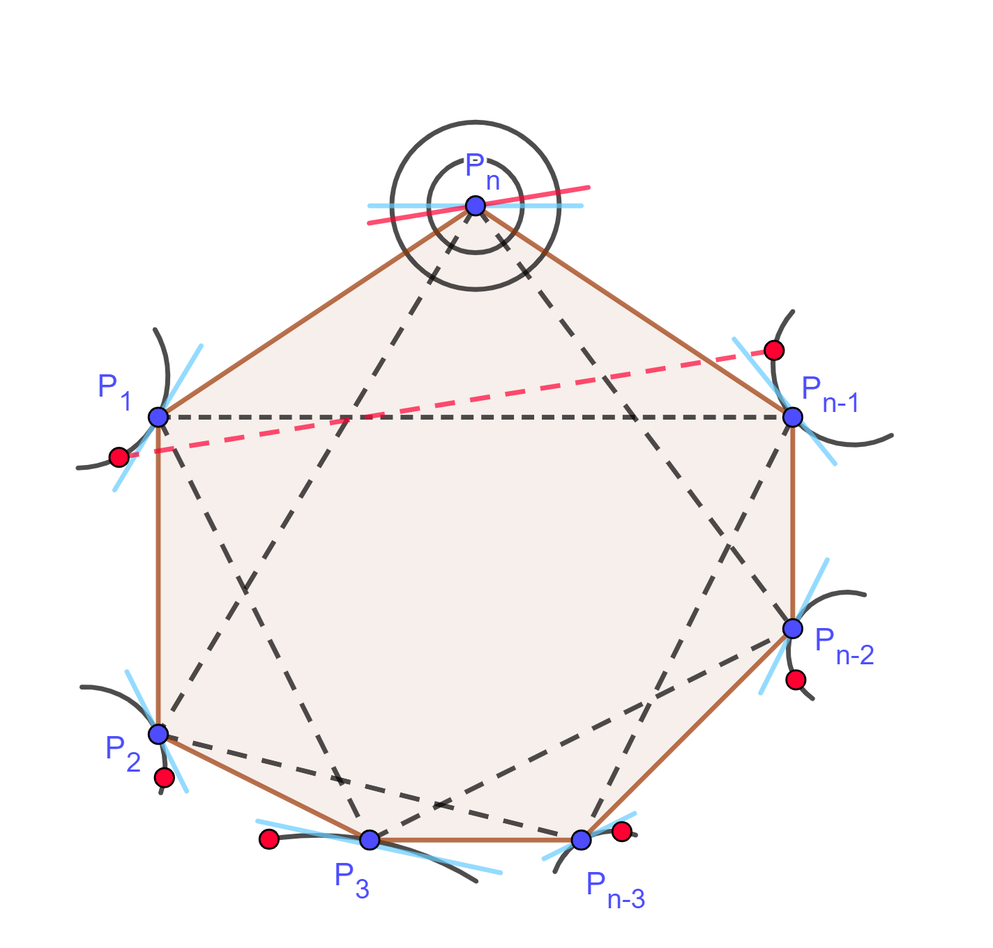
Figure 9. Growing circles

Remark 4.

How to determine the sign of $a_{n}$ in a geometric way ? Let $M_{i}$ be the center of curvature of $C_{i}$ at the point $P_{i}$ then $a_{i}>0$ if $M_{i}$ is on the left side of the tangent line and $a_{i}<0$ if $M_{i}$ is on the right side. (the tangent line has orientation from $P_{i-1}P_{i+1}$).

Remark 5.

In case $a_{n}\det H_{n-1}\neq 0$ the formula (6) shows that $\det H[r]=0$ has 2 different roots as soon as $K\neq 0$. It follows, that if $|r|$ grows we get another sign for $H[r]$, which has an effect on the Morse index.

We can extend the idea behind the proof to the growing of more points at the same moment.

Example 1.

We start with a polygon $\mathcal{P}=P_{1}\cdots P_{n}$ in ‘general position”. The directions of the small diagonals determine potential tangent directions. Consider ‘reference’ circles with centers $M_{i}$ and radius $r_{i}$; each of them with a given sign of $a_{i}$ and tangent at $P_{i}$ to the tangent lines. Next consider the circles with center $M_{i}[s]$ and radius $sr_{i}$, still tangent to the same tangent line which coincide for $r=1$ with our reference circle’s.

Our polygon is critical for every $s$. The matrix elements are $a_{i}[s]=sa_{i}$ and $b_{i}[s]=s^{2}b_{i}$, where the $a_{i}$ and $b_{i}$ are defined for the reference circles.

It follows ($k=1,\cdots n$):

$$\det H_{k}[s]=s^{k}(a_{1}a_{2}\cdots a_{k}+s^{2}K_{k}[s])$$

For small enough $s>0$ the sign is given by the sign of $a_{1}a_{2}\cdots a_{k}$. With the help of the Sylvester rule one can compute the index of the critical polygon. By changing the signs of $a_{i}$ (taking the reference circle at the other side of the tangent line) one changes the index. By repeating this procedure one can get any index.

4.3. The birth of centered circles

The circles in Proposition 8 don’t have the center in $P_{i}$. The following statement tells about that situation (see the right hand side of Fig 9): Let $C_{1},\cdots,C_{n-1}$ be curves and $C_{n}$ is a point curve $P_{n}$ (all disjoint). Let the point $P_{n}$ grow to a small circle $C(P_{n},r)$. We look for the critical points of $\mathcal{A}$: It turns out that generically each critical point on $W=C_{1}\times\cdots\times C_{n-1}$ generates two critical points on $W\times S^{1}$:

Proposition 9.

Given points $P_{1},\cdots,P_{n-1}$ on smooth curves $C_{1},\cdots,C_{n-1}$ and a point $P_{n}$ such that the polygon $P_{1}P_{2}\cdots P_{n-1}P_{n}$ is a critical point of $\mathcal{A}$ on $W$.
Assume transversality: $P_{i-1}P_{i+1}\pitchfork P_{i}P_{i+2}$ for $i=1,\cdots,n$. Then, for $r$ small enough, there exists near to $P_{1}P_{2}\cdots P_{n-1}P_{n}$ on $W\times C(P_{n},r)$ exactly two critical polygons $P_{1}^{\pm}\cdots P_{n-1}^{\pm}P_{n}^{\pm}$, where $P_{n}^{\pm}$ on $C(P_{n},r)$.
If the original critical point is Morse of index $\mu$ then the two new critical points are again Morse and have index $\mu$, resp. $\mu+1$.

Proof.

We start with a billiard type construction. Our reasoning applies to local neighbourhoods of the points $P_{1},\cdots,P_{n}$. The transversality conditions imply that each line $P_{i-1}P_{i+1}$ intersects $C_{i-1}$, resp $C_{i+1}$ transversal at $P_{i-1}$, resp $P_{i+1}$, $(i=2,\cdots,n-2)$,
Choose coordinates $t_{1},t_{2}$ on $C_{1},C_{2}$ such that $P_{1}$ and $P_{2}$ correspond to $t_{i}=0$. Next we define $t_{3},\cdots,t_{n-2}$ such that

$$C_{i}(t_{i})C(t_{i+2})\parallel\mathbb{R}C_{i+1}^{{}^{\prime}}(t_{i+1})\;\;,\;(i=1,\cdots n-2.)$$

Due to the transversality conditions, this well defined in a neighbourhood of $(0,0)$. The maps $(t_{i},t_{i+1})\rightarrow(t_{i+1},t_{i+2})$ are local diffeomorphisms by the same reason.

We intend to use $(t_{1},t_{2})$ as a coordinate system near $P_{n}$. Consider the map

$$(t_{1},t_{2})\rightarrow Q(t_{1},t_{2})=\big{(}C_{2}(t_{2})+\mathbb{R}C_{1}^{{}^{\prime}}(t_{1})\big{)}\cap\big{(}C_{n-2}(t_{n-2})+\mathbb{R}C_{n-1}^{{}^{\prime}}(t_{n-1})\big{)}.$$

Also this map is a local diffeomorphism, due to the transversality of the images of the two coordinate-axis, which intersect in $Q=P_{n}$. Let $\Phi(X)=(t_{1}(X),t_{2}(X))$ be its inverse.
Next parametrize $C(P_{n},r)$ by $X(t)=P_{n}+r(\cos t,\sin t)$ , $t\in[0,2\pi]$. While $X$ is moving around the circle, we consider the argument $\beta_{r}(t)$ of the chord from $C_{n-1}(t_{n-1}(X))$ to $C_{1}(t_{1}(X))$. Note that for $r$ small enough the image of $\beta_{r}$ is contained in an arbitrary small circle sector around the (limit) direction $\beta_{0}$.
In order to satisfy the parallel condition between $C_{1}$ and $C_{n-1}$ we have to determine those points $X$ on $C(P_{n},r)$ where the tangent line to the circle is parallel to the chord. This is given by the condition $t-\beta_{r}(t)=\pm\pi/2$. For $r$ small enough the graph of $t-\beta_{r}(t)$ is transversal to levels $\pm\pi/2$, since this is the case if $r=0$ and moreover the 2 points of intersection survive during the small deformation. Since our constructing takes care of all other parallel conditions we have shown that the two resulting polygons are critical.

The statement about the Morse indices in $P_{n}^{\pm}$ follows in the same way as in Proposition 8. The entries in the formula (6) now depend all on $r$, but for $r$ small enough $a_{n}$ and $\det H_{n-1}$ are bounded away from $0$.

∎

5. Polygons on a single curve

5.1. Local, global and zigzags

The case of a single curve is of special interest. In this case we meet also non-isolated singularities of the area function, due to coinciding vertices. If all vertices are distinct, then $\mathcal{A}$ behaves as if the vertices were on different local curves and we can use all the facts about these from the proceeding sections. We call these the global case, while coinciding vertices are related to local effects. This can give rise to a zig-zag behaviour of critical polygons.

Definition 1.

Adding a zig-zag to a n-gon $\mathcal{P}=P_{1}P_{2}\cdots P_{n}$ is a the (n+2)-gon $\overline{\mathcal{P}}=P_{1}\cdots P_{i-1}P_{i}P_{i-1}P_{i}P_{i+1}\cdots P_{n}$

Note that the $i^{th}$ condition for critical polygons has two aspects:

• $P_{i+1}=P_{i-1}$ or

• $T(P_{i})\parallel P_{i-1}P_{i+1}$

Therefore we have:

Proposition 10.

Let $\mathcal{P}$ be a critical n-gon on $C$, then any (n+2)-gon $\overline{\mathcal{P}}$ with a zigzag added to $\mathcal{P}$ is also critical on $C$.

N.B. We meet a similar behaviour in case of two curves $C_{even},C_{odd}$, where the vertices are on the corresponding curve: $P_{i}\in C_{even}$ when $i$ is even, and $P_{i}\in C_{odd}$ when $i$ is odd.

The next statement works in the generic case:

Proposition 11.

If the critical polygon $\mathcal{P}$ is Morse and $C_{n-1}^{{}^{\prime}}\times C_{n}^{{}^{\prime}}\neq 0$ then $\overline{\mathcal{P}}$ is also critical and Morse and:     Morse-index $(\overline{\mathcal{P}})=1+$ Morse-index $({\mathcal{P}})$

Proof.

We can assume that $i=n$, so $\overline{\mathcal{P}}=P_{1}P_{2}\cdots P_{n-1}P_{n}P_{n-1}P_{n}$ We compare the Hessian matrices: For $n=5$ these are as follows:

$$H=\begin{pmatrix}a_{1}&b_{1}&0&0&b_{5}\\ b_{1}&a_{2}&b_{2}&0&0\\ 0&b_{2}&\ a_{3}&b_{3}&0\\ 0&0&b_{3}&a_{4}&b_{4}\\ b_{5}&0&0&b_{4}&a_{5}\end{pmatrix}\;\;;\;\;\overline{H}=\begin{pmatrix}a_{1}&b_{1}&0&0&0&0&b_{5}\\ b_{1}&a_{2}&b_{2}&0&0&0&0\\ 0&b_{2}&\ a_{3}&b_{3}&0&0&0\\ 0&0&b_{3}&a_{4}&b_{4}&0&0\\ 0&0&0&b_{4}&a_{5}&-b_{4}&0\\ 0&0&0&0&-b_{4}&0&b_{4}\\ b_{5}&0&0&0&0&b_{4}&0\end{pmatrix}$$

Notice that we get two extra rows and columns. The entries in the new row and columns are 0 on the main diagonal . Due to the zigzag we have that three tangent vectors are the same or have opposite direction. As a consequence:
$\overline{b}_{n+2}=b_{n}\;,\;\overline{b}_{n+1}=b_{n-1}\;,\;\overline{b}_{n}=-b_{n-1}$, $a_{n+1}=a_{n+2}=0.$

We apply Sylvester’s rule for our Hessian $H$ and compare the sequence ( 5)

$$1,\det H_{1},\det H_{2},\cdots,\det H_{n-1},\det H_{n}$$

with the corresponding sequence for $\overline{H}$:

$$1,\det\overline{H}_{1},\det\overline{H}_{2},\cdots,\det\overline{H}_{n-1},\det\overline{H}_{n},\det\overline{H}_{n+1},\det\overline{H}_{n+2}$$

Due to our genericity assumption both sequences satisfy the Sylvester assumptions. Note that : $H_{k}=\overline{H}_{k}$ as soon as $k\leq n-1$. Moreover by elementary determinant operations:
$\det\overline{H}_{n+2}=-b_{n-1}^{2}\det H_{n}$,
$\det\overline{H}_{n+1}=-b_{n-1}^{2}\det H_{n-1}.$
Let $\epsilon_{k}$ be the sign of $\det H_{k}$. The sign sequences of the two determinant sequence above are as follows:
$+,\epsilon_{1},\epsilon_{2},\cdots,\epsilon_{n-1},\epsilon_{n}$,
$+,\epsilon_{1},\epsilon_{2},\cdots,\epsilon_{n-1},\rho\;,-\epsilon_{n-1},-\epsilon_{n}$.
where $\rho$ is the sign of $\overline{H}_{n}$. It is clear that independent of the value $\rho$ the number of sign changes in the second sequence is one more than in the first. ∎

In the case of even $n$ one can meet so-called zigzag-trains (as in the circle case, discussed in ([Si])): Start with $P_{1}$ and $P_{2}$: construct $P_{3}$ by the parallel criterion, and continue in this way: $P_{4}$, etc. For some $k$ switch to the condition $P_{k+1}=P_{k-1}$ and continue with $P_{k+2}=P_{k-2}$ until we arrive in $P_{1}$. One can also put some zig-zags in between (does not matter where). By moving $P_{1}$ and $P_{2}$ one gets 2-dimensional families of polygons: zigzag trains.

Special zigzag-trains arise from two different points on the curve. The 2-gon $P_{1}P_{2}$ is always critical. Adding zigzags give critical 4-gons $P_{1}P_{2}P_{1}P_{2}$, etc. a series of non-isolated critical polygons. Also the case when all points coincide is a non-isolated critical polygon. So there are plenty of non-isolated critical polygons! Their (Bott)-Morse theory can become very complicated.

5.2. Polygons in a circle or ellipse

In [Si] we give a complete description of all critical polygons and indices. The main theorem gives geometric criteria for the critical points and determines also the Hesse matrix at those points. Most of the critical points are of Morse type and look as a regular star, but several of them have zigzag behaviour. The Morse index is determined by combinatorial data. We give a summarized version where $\alpha_{i}=\angle P_{i}MP_{i+1}$ and $M$ is the center of the circle.

Theorem 2.

The signed area function for polygons on a circle (defined on the reduced configuration space) has critical points iff all $|\alpha_{i}|$ are equal. These critical points are isolated or (if the number of vertices $n=$ even) contain also a 1-dimensional singular set. More precise

• The isolated singularity types are regular stars, zigzag stars and if $n=$odd also degenerate stars,

• All regular and zigzag stars are Morse critical points,

• Degenerate stars are degenerate isolated critical points if $n$ is odd.

• The non-isolated case only occurs if n = even and includes the complete fold, zigzag trains and degenerate stars. The non-isolated part of the critical set contains $\tbinom{n}{\frac{n}{2}}$ branches, which meet only at the complete fold and the degenerate stars.

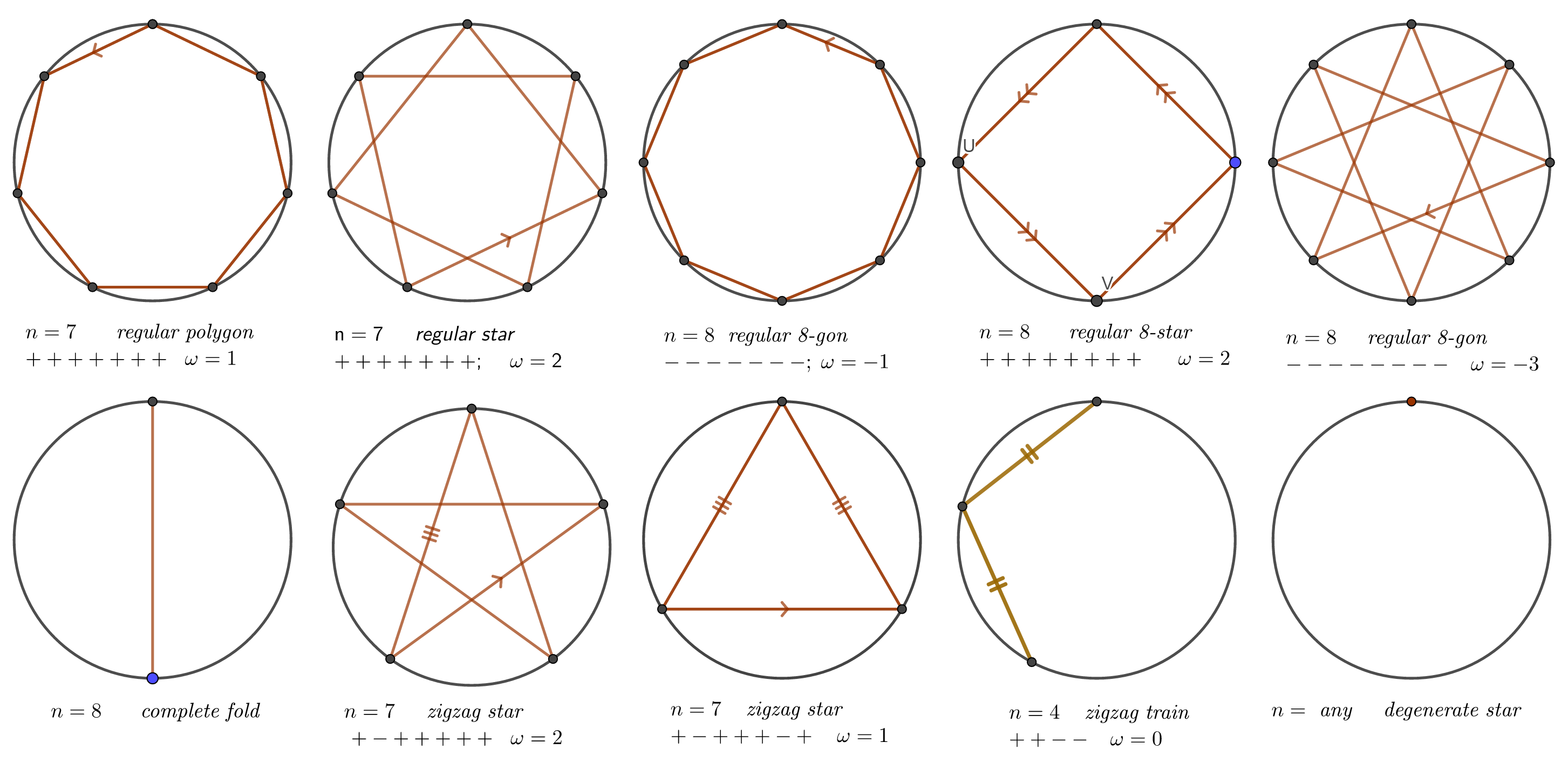
Figure 10. Some critical configurations

We computed also the index of the gradient vector field at the degenerate star by Euler-characteristic arguments. In section 3 of [Si] we discussed the Eisenbud-Levine-Khimshiashvili method to calculate this index. This related nicely to a combinatorial question, which is solved in [vdKS].

Note, that the problem of extremal area polygons in an ellipse is also solved due to the existence of an area preserving affine map.

6. Piecewise differentiable curves

In many situations piecewise smooth curves occur. These are differentiable curves with finitely many (break) points, where only the right-derivative and the left derivative exist, $C_{i,-}^{{}^{\prime}}$, resp. $C_{i,+}^{{}^{\prime}}$. We denote the corresponding tangent vectors by $T_{i,-}$, resp $T_{i,+}$.

We can determine the critical points of $\mathcal{A}$ with the help of generalized derivatives, e.g. the Clark subdifferential. The generalized derivative of $C(t)$ at a break point is given by $\delta C=ch(T_{-},T_{+})$, the convex hull of the right and the left tangent vector; the corresponding cone in the tangent spaces is denote by $TC$. We avoid $T_{-}+T_{+}=0$ !

The area function $\mathcal{A}$ is an example of a ‘continuous selection’. Its critical point and Morse theory are especially studied in [JP] and [APS]. A continuous function $f$ is called a continuous selection of functions $f_{1},\cdots,f_{m}$ if $I(x)=\{i\in\{1,\cdots,m\}|f_{i}(x)=f(x)\}$ is non-void . The set $I(x)$ is called the active index set of $f$ at the point $f$.

If all the functions $f_{i}$ are smooth ($C^{1}$ ) then $f$ is locally Lipschitz continuous and the Clark subdifferental of $f$ is given by

$$\delta f(x)=ch\{\nabla f_{i}(x)|i\in\hat{I}(x\},$$

where $\hat{I}(x)=\{i|x\in cl\;int\{x|f(x)=f_{i}(x)\}\}$.
Subdifferentials satisfy the usual calculus rules: vectors replaced by sets.

A point $x_{0}$ is called a critical point of a locally Lipschitz continuous function iff $O\in\delta f(x_{0})$.
Locally Lipschitz continuous functions satisfy the first Morse lemma: No critical points imply a (topological) product structure. We apply this to $\mathcal{A}$:

Theorem 3.

Let $C_{1},\cdots,C_{n}$ be piecewise smooth curves in the plane. $\mathcal{A}$ has a critical point at the polygon $P_{1}\cdots P_{n}$ iff $O\in\delta C_{i}\times(C_{i+1}-C_{i-1})$ for all $i$ at $(t_{1},\cdots,t_{n}.$ with $P_{i}=C(t_{i})$
This means:

• $P_{i+1}=P_{i-1}$ or

• $P_{i-1}P_{i+1}\in TC(P_{i})$

The paralell condition is now replaced by the tangent cone condition (Figure 11).

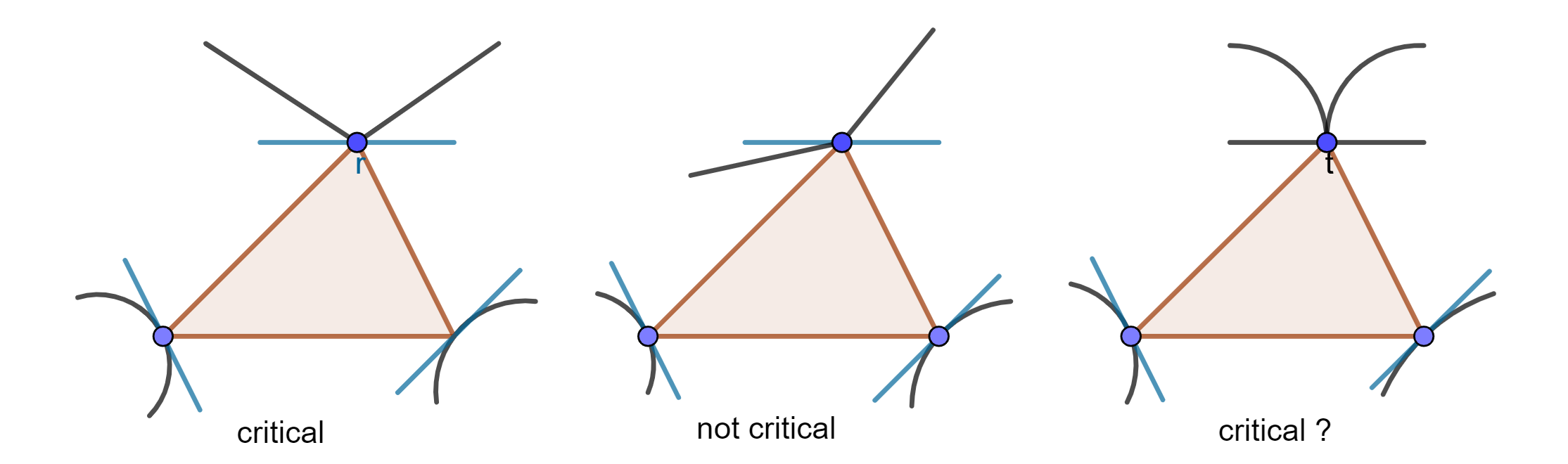
Figure 11. Non smooth critical points.

We don’t treat the Morse theory, we restrict ourselves to the following remarks: Morse theory for continuous selections is developed in [APS], but in the case of the area function $\mathcal{A}$ an extension seems to be necessary.
A second approach can be sketched as follows. Use a rounding off curve $\tilde{C}_{i}$ of $C_{i}$ in a very small neighbourhood of the breakpoints. It is clear that the critical points of $\mathcal{A}$ in the two situations are in 1-1 correspondence. We expect even that $\mathcal{A}$ in the two cases is topologically equivalent. Next one can use smooth Morse theory to determine the type of the critical points. We leave this idea for further studies. It seems interesting in the case that each $C_{i}$ is a polygon, especially in the case of coinciding curves.

The triangle case is intensively studied in computational geometry. Mostly to invent algorithms to select the maximal area triangle in a polygon with many vertices. It could be of interest to study the critical point theory of triangles, 4-gons and higher. One can also meet non-isolated singularities. Is it possible to use the simplicial structure and discrete Morse theory ?

7. Tangential sliding

7.1. Critical Points

We us the notations $C_{1},\cdots,C_{n}$ for the curves, which we give a direction and a parametrization.

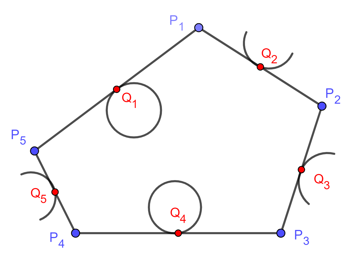
Figure 12. Tangential polygon in midpoint position

On each of the curves we consider a point $Q_{i}$. The tangent lines in $Q_{i}$ define a polygon, by taking the intersection points $P_{i}$ between the tangent lines in $Q_{i}$ and $Q_{i+1}$. The signed area of $P_{1}P_{2}\cdots P_{n}$ defines a function $t\mathcal{A}:(S^{1})^{n}\to\mathbb{R}$ . The point $Q_{i}$ is not defined if the two tangent lines are parallel. One could probably add the values $\pm\infty$ to the source space.

Theorem 4.

Critical points of $t\mathcal{A}$ are polygons where the vertices are midpoints or points with vanishing curvature.

Proof.

$t\mathcal{A}$ depends on $(t_{1},\cdots,t_{n})$. Fix next all $t_{k}$ with $k\neq i$ and compute the partial derivative with respect to $t_{i}$. It is sufficient to consider the triangle $Q_{i-1}Q_{i}Q_{i+1}$. The statement for triangles is folklore (see 7.2) and follows by elementary computations. ∎

7.2. Triangle case

More than 100 years ago E.B. Wilson [Wi] showed, that for triangles on convex curves vertex area $\mathcal{A}$ and tangential area $t\mathcal{A}$ have the same critical points. He used an infinitesimal proof and asked the question: Is there any ‘easy’ way of reaching this result by exclusively analytic methods now in vogue ?. This follows now anyhow from our Theorem 1 and Theorem 4. By elementary geometry the midpoint condition for the tangential triangle and the parallel condition are equivalent.

If $n>3$ there is no longer the coincidence of critical points for both type of slidings.

7.3. Related work

In the paper [CMD] one considers given angles of the polygon and give geometric conditions for extremal perimeter and area. The paper [dT] contains not only criteria for extermal perimeter, but at the end also for area. The midpoint condition is contributed to M.M. Day (1974).

8. Towards an Inner Area Billiard

The critical polygon construction for the area function $\mathcal{A}$ can be used to define a new billiard. The approach will be similar to the constructions of (usual) billiard from the perimeter function

$$\mathcal{P}er=|P_{1}P_{2}|+|P_{2}P_{3}|+\cdots|P_{n-1}P_{n}|+P_{n}P_{1}|$$

and the outer billiard as explained below. We describe both in cases of a differentiable strict convex curve $C$. As references to billiards we give [Ta] and [GT].

8.1. (Inner) Perimeter Billiard

For polygons on $C$ the critical points of $\mathcal{P}er$ are determined by the reflection law: Two consecutive edges reflect in the tangent line at the common vertex. One can use the same rule for construction of the billiard. Start with $P_{1}\neq P_{2}$ on $C$, determine $P_{3}$ via the reflection rule in $P_{2}$ as intersection of the reflected ray with $C$, etc. The closed orbits correspond to the critical points of $\mathcal{P}er$. To distinguish from other billiards we will call this the Inner Perimeter Billiard.

8.2. (Outer)Area Billiard

Next we consider polygons where the edges are tangent to the curve $C$. The critical points of $t\mathcal{A}$ are determined by the mid-point property: Any edge is tangent to $C$ at its mid-point (Theorem 4). The Outer Area Billiard is defined by that rule : Start with any point $P_{1}$ outside the convex region , draw a tangent line to $C$ (there are 2 choices) and take the point $P_{2}$ on the tangent line such that the point of tangency is the mid-point. Construct $P_{3}$ via the (other) tangent line to $C$ and $\cdots$, etc. The closed orbits correspond to the critical points of (outer) area $t\mathcal{A}$.

8.3. Inner Area Billiard

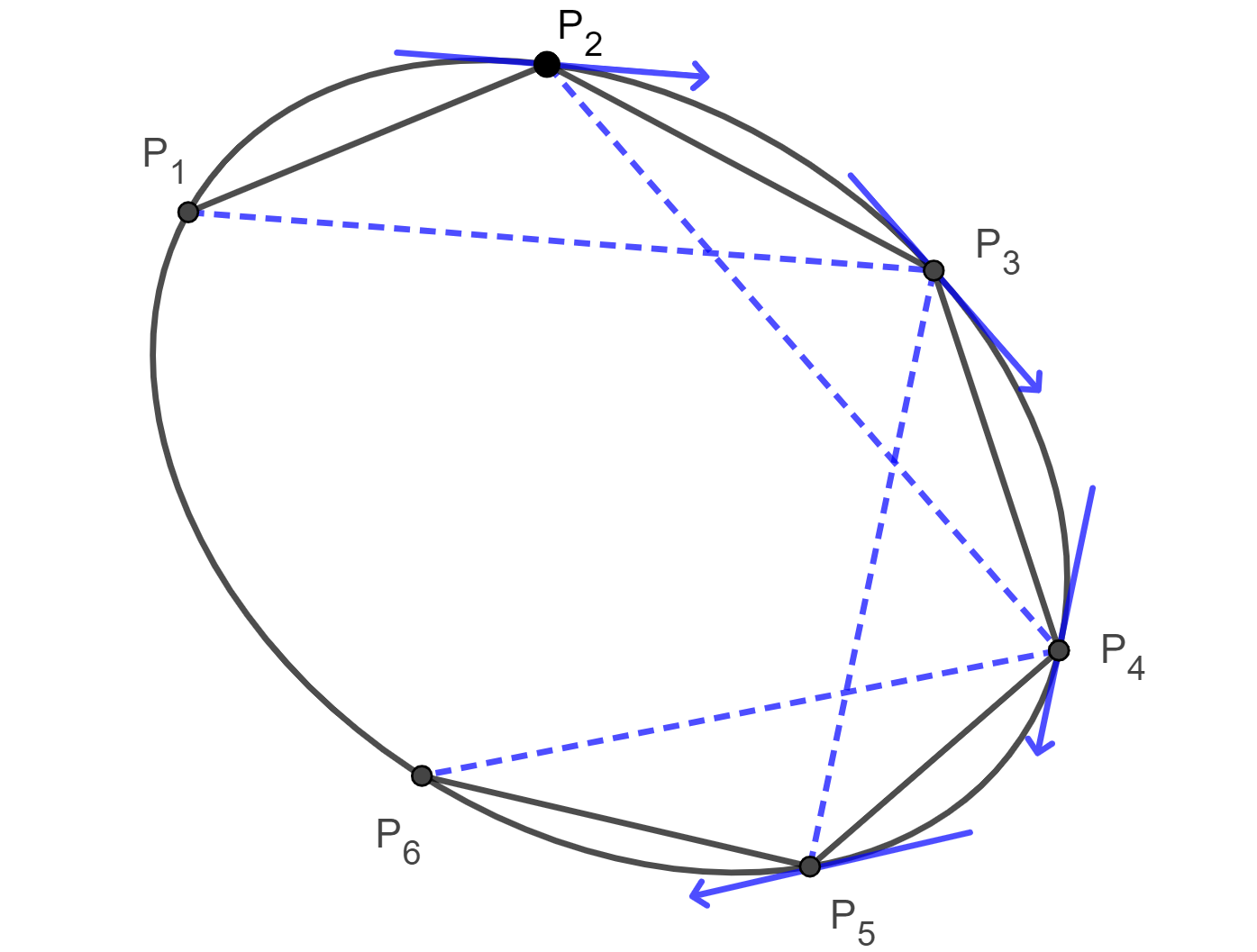
Figure 13. The inner area billiard.

Now we describe our new billiard by using the (inner) area function $\mathcal{A}$. Start with a polygon inscribed in a convex curve. The critical points of $\mathcal{A}$ are given by the parallel rule:
$T(P_{i})\parallel P_{i-1}P_{i+1}\;\;,i=1,\cdots n$. We exclude the zigzag-rule.

Start with $P_{1}\neq P_{2}$ on the curve and construct $P_{3}$ by intersecting the line through $P_{1}$ parallel to $T(P_{2})$ with $C$, construct $P_{4}$ by intersecting the line through $P_{2}$ parallel to $T(P_{3})$, etc. The closed orbits are the critical polygons of (inner) area $\mathcal{A}$. We call this billiard the Inner Area Billiard.

It looks interesting to study the properties of this billiard in detail. Questions are:

• Do caustics exist ?

• Existence of closed n-orbits with given winding number

• Other questions in ordinary billiard theory

Note that the area function on the ellipse has the property that it has a caustic which is again an ellipse. Each critical polygon is non-isolated. The types of critical orbits follow from [Si]. The caustic exists and is also an ellipse.

References

- [APS] A.A. Agracev, D. Pallaschke, S. Scholtes, On Morse theory for piecewise smooth functions, Journal of Dynamical and Control Systems, Vol 3, no. 4, 1997, 4449-469 ,
- [Bl] V. Blåsjö, The isoperimetric problem, American Mathematical Monthly, 112, 6 (2005), 525-566.
- [CMD] W. Ciéslak, M. Maksym, D. DeTemple, On polygons circumscribing a close convex curve, Journal of geometry Vol 40 (1991), 26-34.
- [dT] D. DeTemple, The geometry of circumscribing polygons of minimal perimeter, Journal of Geometry, Vol 49 (1994) p. 72-89.
- [GR] E. Ghys, A. Ranicki, Signatures in algebra, topology and dynamics Ensaios Mat., 30, Soc. Brasil. Mat., Rio de Janeiro, 2016.
- [GP] V. Guillemin, A Pollack, Differential Topology,Prentice Hall, 1974.
- [GT] D. Genin, S. Tabachnikov, On configuration spaces of plane polygons, sub-Riemannian geometry and periodic orbits of outer billiards, Journal of Modern Dynamics, Vol 1 (2006), p.155-173.
- [JP] H. Th. Jongen, D. Pallaschke, On linearization and continous selecctions of functions Optimiz. 19 (1988), No. 3, 343-353.
- [vdKS] W. van der Kallen, D. Siersma, Subset representations and eigenvalues of the universal intertwining matrix Journal of Pure and Applied Algebra, volume 226 (2022), issue 8, pp. 1 - 6.
- [KPS] G. Khimshiashvili, G. Panina, D. Siersma, Extremal Area’s of Polygons with Fixed Perimeter. Zap. Nauchn. Sem. S.-Petersburg. Otdel. Mat. Inst. Steklov. (POMI), 2019, 841, 136-145.
- [KP] G. Khimshiashvili, G. Panina, Cyclic polygons are critical points of area. Zap. Nauchn. Sem. S.-Peterburg. Otdel. Mat. Inst. Steklov. (POMI), 2008, 360, 8, 238–245.
- [KS1] G. Khimshiashvili, D. Siersma, Critical Configurations of planar Multiple Penduli. preprint ICTP preprint IC/2009/047.
- [KS2] G. Khimshiashvili, D. Siersma, Critical Configurations of planar Multiple Penduli. Journal of Mathematical Sciences, Volume 195, No. 2, November 2013, p 198-212.
- [PZ] G. Panina, A. Zhukova, Morse index of a cyclic polygon,Cent. Eur. J. Math., 9(2) (2011), 364-377.
- [SV] D. Shimamoto, C. Vanderwaart, Spaces of Polygons in the Plane and Morse Theory The American Mathematical Monthly, Vol. 112, No. 4 (Apr., 2005), pp. 289-310.
- [Si] D. Siersma, Extremal Area of Polygons, sliding along a circle, Hokkaido Mathematical Journal, Vol 51 (2022), 175-187, doi:10.14492/hokmj/2020-312.
- [Ta] S. Tabachnikov, Geometry and Billiards, Providence, RI: American Mathematical Society, ISBN 978-0-8218-3919-5
- [Wi] E.B. Wilson, Relating to Infinitesimal Methods in Geometry, The American Mathematical Monthly, Vol 23, No.5 (May 1917), p. 241-243.