CLIP-ReID: Exploiting Vision-Language Model for Image Re-Identification without Concrete Text Labels

Abstract

Pre-trained vision-language models like CLIP have recently shown superior performances on various downstream tasks, including image classification and segmentation. However, in fine-grained image re-identification (ReID), the labels are indexes, lacking concrete text descriptions. Therefore, it remains to be determined how such models could be applied to these tasks. This paper first finds out that simply fine-tuning the visual model initialized by the image encoder in CLIP, has already obtained competitive performances in various ReID tasks. Then we propose a two-stage strategy to facilitate a better visual representation. The key idea is to fully exploit the cross-modal description ability in CLIP through a set of learnable text tokens for each ID and give them to the text encoder to form ambiguous descriptions. In the first training stage, image and text encoders from CLIP keep fixed, and only the text tokens are optimized from scratch by the contrastive loss computed within a batch. In the second stage, the ID-specific text tokens and their encoder become static, providing constraints for fine-tuning the image encoder. With the help of the designed loss in the downstream task, the image encoder is able to represent data as vectors in the feature embedding accurately. The effectiveness of the proposed strategy is validated on several datasets for the person or vehicle ReID tasks. Code is available at https://github.com/Syliz517/CLIP-ReID.

Introduction

Image re-identification (ReID) aims to match the same object across different and non-overlapping camera views. Particularly, it focuses on detecting the same person or vehicle in the surveillance camera networks. ReID is a challenging task mainly due to the cluttered background, illumination variations, huge pose changes, or even occlusions. Most recent ReID models depend on building and training a convolution neural network (CNN) so that each image is mapped to a feature vector in the embedding space before the classifier. Images of the same object tend to be close, while different objects become far away in this space. The parameters of CNN can be effectively learned under the guidance of cross entropy loss together with the typical metric learning loss like center or triplet loss (Hermans, Beyer, and Leibe 2017).

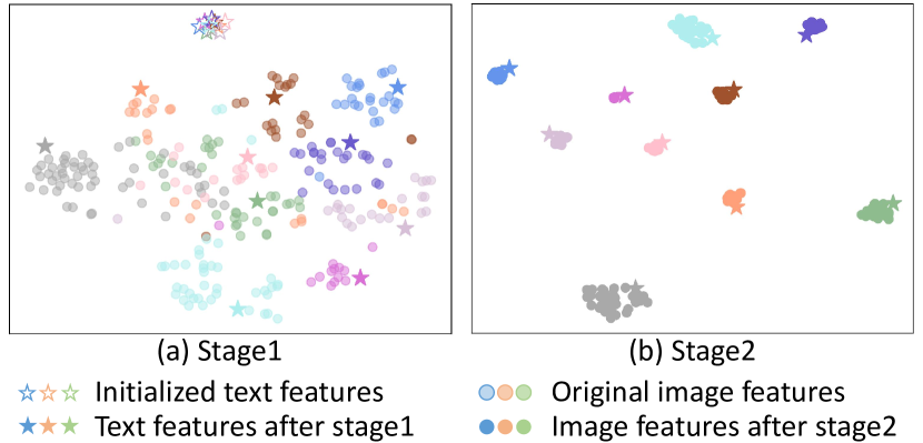
Figure 1: t-SNE visualization on image and text features (Van der Maaten and Hinton 2008). Randomly selected 10 persons in the MSMT17 are represented by different colors. The dots and pentagons indicate the image and text features, respectively. (a) and (b) show the data distributions after the first and second training stage.

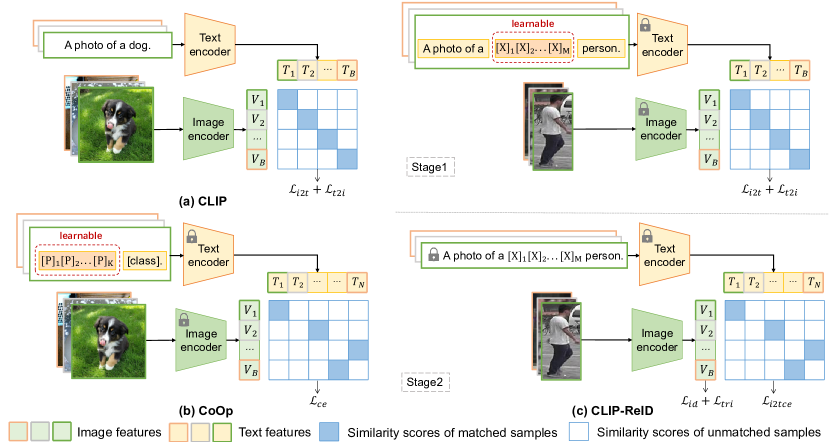
Figure 2: Overview of our approach compared to CLIP and CoOp. (a) describes the model of CLIP, using pairs of text and image to train the image encoder and text encoder. (b) shows the model of CoOp, which fixes the image encoder and text encoder and fine-tunes text prompt in the downstream dataset. (c) is our proposed CLIP-ReID method, which fixes the text encoder and image encoder in the first training stage, optimizes a set of learnable text tokens to generate the text features, and then uses the text features to optimize the image encoder in the second training stage.

Although CNN-based models for ReID have achieved good performance on some well-known datasets, it is still far from being used in a real application. CNN is often blamed for only focusing on a small irrelevant region in the image, which indicates that its feature is not robust and discriminative enough. Recently, vision transformers like ViT (Dosovitskiy et al. 2020) have become popular in many tasks, and they have also shown better performances in ReID. Compared to CNN, transformers can model the long-range dependency in the whole image. However, due to a large number of model parameters, they require a big training set and often perform erratically during optimization. Since ReID datasets are relatively small, the potential of these models is not fully exploited yet.

Both CNN-based and ViT-based methods heavily rely on pre-training. Almost all ReID methods need an initial model trained on ImageNet, which contains images manually given one-hot labels from a pre-defined set. Visual contents describing rich semantics outside the set are completely ignored. Recently, cross-modal learning like CLIP (Radford et al. 2021) connects the visual representation with its corresponding high-level language description. They not only train on a larger dataset but also change the pre-training task, matching visual features to their language descriptions. Therefore, the image encoder can sense a variety of high-level semantics from the text and learns transferable features, which can be adapted to many different tasks. E.g., given a particular image classification task, the candidate text labels are concrete and can be combined with a prompt, such as “A photo of a”, to form the text descriptions. The classification is then realized by comparing image features with text features generated by the text encoder, which takes the text description of categories as input. Note that it is a zero-shot solution without tuning any parameters for downstream tasks but still gives satisfactory results. Based on this, CoOp (Zhou et al. 2021) incorporates a learnable prompt for different tasks. The optimized prompt further improves the performance.

CLIP and CoOp need text labels to form text descriptions in downstream tasks. However, in most ReID tasks, the labels are indexes, and there are no specific words to describe the images, so the vision-language model has not been widely adopted in ReID. In this paper, we intend to exploit CLIP fully. We first fine-tune the image encoder by directly using the common losses in ReID, which has already obtained high metrics compared to existing works. We use this model as our baseline and try to improve it by utilizing the text encoder in CLIP. A two-stage strategy is proposed, which aims to constrain the image encoder by generating language descriptions from the text encoder. A series of learnable text tokens are incorporated, and they are used to describe each ID ambiguously. In the first training stage, both the image and text encoder are fixed, and only these tokens are optimized. In the second stage, the description tokens and text encoder keep static, and they together provide ambiguous descriptions for each ID, which helps to build up the cross-modality image to text cross-entropy loss. Since CLIP has CNN-based and ViT-based models, the proposed method is validated on both ResNet-50 and ViT-B/16. The two types of the model achieve the state-of-the-art on different ReID datasets. Moreover, our method can also support the input of camera ID and overlapped token settings in its ViT-based version.

Fig. 1 simultaneously visualizes image and text features in 2D coordinates, which could help to understand our training strategy. In the first stage, the text feature of each ID is adapted to its corresponding image features, making it become ambiguous descriptions. In the second stage, image features gather around their text descriptions so that image features from different IDs become distant.

In summary, the contributions of this paper lie in the following aspects:

• To our knowledge, we are the first to utilize CLIP for ReID. We provide competitive baseline models on several ReID datasets, which are the result of fine-tuning the visual model initialized by the CLIP image encoder.

• We propose the CLIP-ReID, which fully exploits the cross-modal describing ability of CLIP. In our model, the ID-specific learnable tokens are incorporated to give ambiguous text descriptions, and a two-stage training strategy is designed to take full advantage of the text encoder during training.

• We demonstrate that CLIP-ReID has achieved state-of-the-art performances on many ReID datasets, including both person and vehicle.

Related Works

Image ReID

Previous ReID works focus on learning discriminative features like foreground histograms (Das, Chakraborty, and Roy-Chowdhury 2014), local maximal occurrences (Liao et al. 2015), bag-of-visual words (Zheng et al. 2015), or hierarchical Gaussian descriptors (Matsukawa et al. 2016). On the other hand, it can also be solved as a metric learning problem, expecting a reasonable distance measurement for inter- and intra-class samples (Koestinger et al. 2012). These two aspects are naturally combined by the deep neural network (Yi et al. 2014), in which the parameters are optimized under an appropriate loss function with almost no intentional interference. Particularly, with the scale development of CNN on ImageNet, ResNet-50 (He et al. 2016) has been regarded as the common model (Luo et al. 2019) for most ReID datasets.

Despite the powerful ability of CNN, it is blamed for its irrelevant highlighted regions, which is probably due to the overfitting of limited training data. OSNet (Zhou et al. 2019) gives a lightweight model to deal with it. Auto-ReID (Quan et al. 2019) and CDNet (Li, Wu, and Zheng 2021) employ network architecture search for a compact model. OfM (Zhang et al. 2021a) proposes a data selection method for learning a sampler to choose generalizable data during training. Although they obtain good results on some small datasets, performances drop significantly on large ones like MSMT17.

Introducing prior knowledge into the network can also alleviate overfitting. An intuitive idea is to use features from different regions for identification. PCB (Sun et al. 2018) and SAN (Qian et al. 2020) divides the feature into horizontal stripes to enhance its ability to represent the local region. MGN (Wang et al. 2018) utilizes a multiple granularity scheme on feature division to enhance its expressive capabilities further, and it has several branches to capture features from different parts. Therefore, model complexity becomes its major issue. BDB (Dai et al. 2019) has a simple structure with only two branches, one for global features and the other for local features, which employs a simple batch feature drop strategy to randomly erase a horizontal stripe for all samples within a batch. CBDB-Net (Tan et al. 2021) enhances BDB with more types of feature dropping. Similar multi-branch approaches (Zhang et al. 2021c; Wang et al. 2022; Zhang et al. 2021b; He et al. 2019; Zhang et al. 2019; Sun et al. 2020) with the purpose of mining rich features from different locations are also proposed, and they can be improved if the semantic parsing map participates during training (Jin et al. 2020b; Zhu et al. 2020; Meng et al. 2020; Chen et al. 2020).

Attention enlarges the receptive field, hence is another way to prevent the model from focusing on small areas. In RGA (Zhang et al. 2020), non-local attention is performed along spatial and channel directions. ABDNet (Chen et al. 2019) adopts a similar attention module and adds a regularization term to ensure feature orthogonality. HOReID (Wang et al. 2020) extends the traditional attention into high-order computation, giving more discriminative features. CAL (Rao et al. 2021) provides an attention scheme for counterfactual learning, which filters out irrelevant areas and increases prediction accuracy. Recently, due to the power of the transformer, it has become popular in ReID. PAT (Li et al. 2021b) and DRL-Net (Jia et al. 2022) build on ResNet-50, but they utilize a transformer decoder to exploit image features from CNN. In the decoder attention block, learnable queries first interact with key tokens from the image and then are updated by weighted image values. They are expected to reflect local features for ReID. TransReID (He et al. 2021), AAformer (Zhu et al. 2021) and DCAL (Zhu et al. 2022) all use encoder attention blocks in ViT, and they obtain better performance, especially on the large dataset.

This paper implements both CNN and ViT models initialized from CLIP. Benefiting from the two-stage training, both achieve SOTA on different datasets.

Vision-language learning.

Compared to supervised pre-training on ImageNet, vision-language pre-training(VLP) has significantly improved the performance of many downstream tasks by training to match image and language. CLIP (Radford et al. 2021) and ALIGN (Jia et al. 2021) are good practices, which utilize a pair of image and text encoders, and two directional InfoNCE losses computed between their outputs for training. Built on CLIP, several works (Li et al. 2022; Kim, Son, and Kim 2021) have been proposed to incorporate more types of learning tasks like image-to-text matching and mask image/text modeling. ALBEF (Li et al. 2021a) aligns the image and text representation before fusing them through cross-model attention. SimVLM (Wang et al. 2021) uses a single prefix language modeling objective for end-to-end training.

Inspired by the recent advances in NLP, prompt or adapter-based tuning becomes prevalent in vision domain CoOp (Zhou et al. 2021) proposes to fit in a learnable prompt for image classification. CoCoOp (Zhou et al. 2022) learns a light-weight visual network to give meta tokens for each image, combined with a set of learnable context vectors. CLIP-Adapter (Gao et al. 2021) adds a light-weight module on top of both image and text encoder.

In addition, researchers investigate different downstream tasks to apply CLIP. DenseCLIP (Rao et al. 2022) and MaskCLIP (Zhou, Loy, and Dai 2021) apply it for per-pixel prediction in segmentation. ViLD (Gu et al. 2021) adapts image and text encoders in CLIP for object detection. EI-CLIP (Ma et al. 2022) and CLIP4CirDemo (Baldrati et al. 2022) use CLIP to solve retrieval problems. However, as far as we know, no works deal with ReID based on CLIP.

Algorithm 1 CLIP-ReID’s training process.

Input: batch of images $x_{i}$ and their corresponding texts $t_{y_{i}}$.
Parameter: a set of learnable text tokens $\rm[X]_{m}$($\rm m\in{1,...M}$) for all IDs existing in training set $\mathcal{X}$, an image encoder $\mathcal{I}$ and a text encoder $\mathcal{T}$, linear layers $g_{V}$ and $g_{T}$.

1:  Initialize $\mathcal{I}$, $\mathcal{T}$, $g_{V}$ and $g_{T}$ from the pre-trained CLIP. Initialize $\rm[X]_{m}$($\rm m\in{1,...M}$) randomly.

2:  while in the 1st stage do

3:     $s(V_{i},T_{y_{i}})=g_{V}(\mathcal{I}(x_{i}))\cdot g_{T}(\mathcal{T}(t_{y_{i}}))$

4:     Optimize $\rm[X]_{m}$ by Eq. 5.

5:  end while

6:  for $y_{i}=1$ to $N$ do

7:     $text_{y_{i}}=g_{T}(\mathcal{T}(t_{y_{i}}))$

8:  end for

9:  while in the 2nd stage do

10:     $s(V_{i},T_{y_{i}})=g_{T}(\mathcal{I}(x_{i}))\cdot text_{y_{i}}$

11:     Optimize $\mathcal{I}$ by Eq. 9.

12:  end while

Method

Preliminaries: Overview of CLIP

We first briefly review CLIP. It consists of two encoders, an image encoder $\mathcal{I}(\cdot)$ and a text encoder $\mathcal{T}(\cdot)$. The architecture of $\mathcal{I}(\cdot)$ has several alternatives. Basically, a transformer like ViT-B/16 and a CNN like ResNet-50 are two models we work on. Either of them is able to summarize the image into a feature vector in the cross-modal embedding.

On the other hand, the text encoder $\mathcal{T}(\cdot)$ is implemented as a transformer, which is used to generate a representation from a sentence. Specifically, given a description such as “A photo of a $\rm[class]$.” where $\rm[class]$ is generally replaced by concrete text labels. $\mathcal{T}(\cdot)$ first converts each word into a unique numeric ID by lower-cased byte pair encoding (BPE) with 49,152 vocab size (Sennrich, Haddow, and Birch 2015). Then, each ID is mapped to a 512-d word embedding. To achieve parallel computation, each text sequence has a fixed length of 77, including the start $\rm[SOS]$ and end $\rm[EOS]$ tokens. After a 12-layer model with 8 attention heads, the $\rm[EOS]$ token is considered as a feature representation of the text, which is layer normalized and then linearly projected into the cross-modal embedding space.

Specifically, $i\in\{1...B\}$ denotes the index of the images within a batch. Let $img_{i}$ be the $\rm[CLS]$ token embedding of image feature, while $text_{i}$ is the corresponding $\rm[EOS]$ token embedding of text feature, then compute the similarity between $img_{i}$ and $text_{i}$:

$$s(V_{i},T_{i})=V_{i}\cdot T_{i}=g_{V}(img_{i})\cdot g_{T}(text_{i})$$ (1)

where $g_{V}(\cdot)$ and $g_{V}(\cdot)$ are linear layers projecting embedding into a cross-modal embedding space. The image-to-text contrastive loss $\mathcal{L}_{i2t}$ is calculated as:

$$\mathcal{L}_{i2t}(i)=-\log\frac{\exp(s(V_{i},T_{i}))}{\sum_{a=1}^{B}\exp(s(V_{i},T_{a}))}$$ (2)

and the text-to-image contrastive loss $\mathcal{L}_{t2i}$:

$$\mathcal{L}_{t2i}(i)=-\log\frac{\exp(s(V_{i},T_{i}))}{\sum_{a=1}^{B}\exp(s(V_{a},T_{i}))}$$ (3)

where numerators in Eq. 2 and Eq. 3 are the similarities of two embeddings from matched pair, and the denominators are all similarities with respect to anchor $V_{i}$ or $T_{i}$.

For regular classification tasks, CLIP converts the concrete labels of the dataset into text descriptions, then produces embedding feature $T_{i}$ , $V_{i}$ and aligns them. CoOp incorporates a learnable prompt for different tasks while entire pre-trained parameters are kept fixed, as depicted in Fig. 2(b). However, it is difficult to exploit CLIP in ReID tasks where the labels are indexes instead of specific text.

CLIP-ReID

To deal with the above problem, we propose CLIP-ReID, which complements the lacking textual information by pre-training a set of learnable text tokens. As is shown in Fig. 2(c), our scheme is built by pre-trained CLIP with the two stages of training, and its metrics exceed our baseline.

The first training stage.

We first introduce ID-specific learnable tokens to learn ambiguous text descriptions, which are independent for each ID. Specifically, the text descriptions fed into $\mathcal{T}(\cdot)$ are designed as “A photo of a $\rm[X]_{1}[X]_{2}[X]_{3}...[X]_{M}$ person/vehicle”, where each $\rm[X]_{m}$($\rm m\in{1,...M}$) is a learnable text token with the same dimension as word embedding. $\rm M$ indicates the number of learnable text tokens. In this stage, we fix the parameters of $\mathcal{I}(\cdot)$ and $\mathcal{T}(\cdot)$, and only tokens $\rm[X]_{m}$ are optimized.

Similar to CLIP, we use $\mathcal{L}_{i2t}$ and $\mathcal{L}_{t2i}$, but replace $text_{i}$ with $text_{y_{i}}$ in Eq. 1, since each ID shares the same text description. Moreover, for $\mathcal{L}_{t2i}$, different images in a batch probably belong to the same person, so $T_{y_{i}}$ may have more than one positive, we change it to:

$$\mathcal{L}_{t2i}(y_{i})=\frac{-1}{|P(y_{i})|}\sum_{p\in P(y_{i})}\log\frac{\exp(s(V_{p},T_{y_{i}}))}{\sum_{a=1}^{B}\exp(s(V_{a},T_{y_{i}}))}$$ (4)

Here, $P(y_{i})=\{p\in{1...B}:y_{p}=y_{i}\}$ is the set of indices of all positives for $T_{y_{i}}$ in the batch, and $|\cdot|$ is its cardinality.

By minimizing the loss of $\mathcal{L}_{i2t}$ and $\mathcal{L}_{t2i}$, the gradients are back-propagated through the fixed $\mathcal{T}(\cdot)$ to optimize $\rm[X]_{1}[X]_{2}[X]_{3}...[X]_{M}$, taking full advantage of $\mathcal{T}(\cdot)$.

$$\mathcal{L}_{stage1}=\mathcal{L}_{i2t}+\mathcal{L}_{t2i}$$ (5)

To improve the computation efficiency, we obtain all the image features by feeding the whole training set into $\mathcal{I}(\cdot)$ at the beginning of the first training stage. For a dataset with $N$ IDs, we save $N$ different $T_{y_{i}}$ of all IDs at the end of this stage, preparing for the next stage of training.

The second training stage.

In this stage, only parameters in $\mathcal{I}(\cdot)$ are optimized. To boost the final performance, we follow the general strong pipeline of object ReID (Luo et al. 2019). We employ the triplet loss $\mathcal{L}_{tri}$ and ID loss $\mathcal{L}_{id}$ with label smoothing for optimization, they are calculated as:

$$\mathcal{L}_{id}=\sum_{k=1}^{N}-q_{k}\log(p_{k})$$ (6)

$$\mathcal{L}_{tri}=\max(d_{p}-d_{n}+\alpha,0)$$ (7)

where $q_{k}=(1-\epsilon)\delta_{k,y}+\epsilon/N$ denotes value in the target distribution, and $p_{k}$ represents ID prediction logits of class $k$, $d_{p}$ and $d_{n}$ are feature distances of positive pair and negative pair, while $\alpha$ is the margin of $\mathcal{L}_{tri}$.

To fully exploit CLIP, for each image, we can use the text features obtained in the first training stage to calculate image to text cross-entropy $\mathcal{L}_{i2tce}$ as is shown in Eq. 8. Note that following $\mathcal{L}_{id}$, we utilize label smoothing on $q_{k}$ in $\mathcal{L}_{i2tce}$.

$$\mathcal{L}_{i2tce}(i)=\sum_{k=1}^{N}-q_{k}\log\frac{\exp(s(V_{i},T_{y_{k}}))}{\sum_{{y_{a}}=1}^{N}\exp(s(V_{i},T_{y_{a}}))}$$ (8)

Ultimately, the losses used in our second training stage are summarized as follows:

$$\mathcal{L}_{stage2}=\mathcal{L}_{id}+\mathcal{L}_{tri}+\mathcal{L}_{i2tce}$$ (9)

The whole training process of the proposed CLIP-ReID, including both the first and second stages, is summarized in Algorithm 1. We use the learnable prompts to mine and store the hidden states of the pre-trained image encoder and text encoder, allowing CLIP to retain its own advantages. During the second stage, these prompts can regularize the image encoder and thus increase its generalization ability.

SIE and OLP.

To make the model aware of the camera or viewpoint, we use Side Information Embeddings (SIE) (He et al. 2021) to introduce relevant information. Unlike TransReID, we only add camera information to the [CLS] token, rather than all tokens, to avoid disturbing image details. Overlapping Patches (OLP) can further enhance the model with increased computational resources, which is realized simply by changing the stride in the token embedding.

Experiments

Datasets and Evaluation Protocols

We evaluate our method on four person re-identification datasets, including MSMT17 (Wei et al. 2018), Market-1501 (Zheng et al. 2015), DukeMTMC-reID (Ristani et al. 2016), Occluded-Duke (Miao et al. 2019), and two vehicle ReID datasets, VeRi-776 (Liu et al. 2016b) and VehicleID (Liu et al. 2016a). The details of these datasets are summarized in Tab. 1. Following common practices, we adapt the cumulative matching characteristics (CMC) at Rank-1 (R1) and the mean average precision (mAP) to evaluate the performance.

Implementations

Models.

We adopt the visual encoder $\mathcal{I}(\cdot)$ and the text encoder $\mathcal{T}(\cdot)$ from CLIP as the backbone for our image and text feature extractor. CLIP provides two alternatives $\mathcal{I}(\cdot)$, namely a transformer and a CNN with a global attention pooling layer. For the transformer, we choose the ViT-B/16, which contains 12 transformer layers with the hidden size of 768 dimensions. To match the output of the $\mathcal{T}(\cdot)$, the dimension of the image feature vector is reduced from 768 to 512 by a linear layer. For the CNN, we choose ResNet-50, where the last stride changes from 2 to 1, resulting in a larger feature map to preserve spatial information. The global attention pooling layer after ResNet-50 reduces the dimension of the embedding vectors from 2048 to 1024, matching the dimensions of the text features converted from 512 to 1024.

Dataset	Image	ID	Cam + View
MSMT17	126,441	4,101	15
Market-1501	32,668	1,501	6
DukeMTMC-reID	36,411	1,404	8
Occluded-Duke	35,489	1,404	8
VeRi-776	49,357	776	28
VehicleID	221,763	26,267	-

Table 1: Statistics of datasets used in the paper.

Training details.

In the first training stage, we use the Adam optimizer for both the CNN-based and the ViT-based models, with a learning rate initialized at $3.5\times 10^{-4}$ and decayed by a cosine schedule. At this stage, the batch size is set to 64 without using any augmentation methods. Only the learnable text tokens $\rm[X]_{1}[X]_{2}[X]_{3}...[X]_{M}$ are optimizable. In the second training stage (same as our baseline), Adam optimizer is also used to train the image encoder. Each mini-batch consists of $\rm B=P\times K$ images, where $\rm P$ is the number of randomly selected identities, and $\rm K$ is samples per identity. We take $\rm P=16$ and $\rm K=4$. Each image is augmented by random horizontal flipping, padding, cropping and erasing (Zhong et al. 2020). For the CNN-based model, we spend 10 epochs linearly increasing the learning rate from $3.5\times 10^{-6}$ to $3.5\times 10^{-4}$, and then the learning rate is decayed by 0.1 at the 40th and 70th epochs. For the ViT-based model, we warm up the model for 10 epochs with a linearly growing learning rate from $5\times 10^{-7}$ to $5\times 10^{-6}$. Then, it is decreased by a factor of 0.1 at the 30th and 50th epochs. We train the CNN-based model for 120 epochs while the ViT-based model for 60 epochs. For the CNN-based model, we use $\mathcal{L}_{tri}$ and $\mathcal{L}_{id}$ pre and post the global attention pooling layer, and $\alpha$ is set to 0.3. Similarly, we use them pre and post the linear layer after the transformer. Note that we also employ $\mathcal{L}_{tri}$ after the 11th transformer layer of ViT-B/16 and the 3rd residual layer of ResNet-50.

Backbone	Methods	References	MSMT17		Market-1501		DukeMTMC		Occluded-Duke
			mAP	R1	mAP	R1	mAP	R1	mAP	R1
CNN	PCB*	ECCV (2018)	-	-	81.6	93.8	69.2	83.3	-	-
	MGN*	MM (2018)	-	-	86.9	95.7	78.4	88.7	-	-
	OSNeT	ICCV (2019)	52.9	78.7	84.9	94.8	73.5	88.6	-	-
	ABD-Net*	ICCV (2019)	60.8	82.3	88.3	95.6	78.6	89.0	-	-
	Auto-ReID*	ICCV (2019)	52.5	78.2	85.1	94.5	-	-	-	-
	HOReID	CVPR (2020)	-	-	84.9	94.2	75.6	86.9	43.8	55.1
	ISP	ECCV (2020)	-	-	88.6	95.3	80.0	89.6	52.3	62.8
	SAN	AAAI (2020b)	55.7	79.2	88.0	96.1	75.5	87.9	-	-
	OfM	AAAI (2021a)	54.7	78.4	87.9	94.9	78.6	89.0	-	-
	CDNet	CVPR (2021)	54.7	78.9	86.0	95.1	76.8	88.6	-	-
	PAT	CVPR (2021b)	-	-	88.0	95.4	78.2	88.8	53.6	64.5
	CAL*	ICCV (2021)	56.2	79.5	87.0	94.5	76.4	87.2	-	-
	CBDB-Net*	TCSVT (2021)	-	-	85.0	94.4	74.3	87.7	38.9	50.9
	ALDER*	TIP (2021b)	59.1	82.5	88.9	95.6	78.9	89.9	-	-
	LTReID*	TMM (2022)	58.6	81.0	89.0	95.9	80.4	90.5	-	-
	DRL-Net	TMM (2022)	55.3	78.4	86.9	94.7	76.6	88.1	50.8	65.0
	baseline		60.7	82.1	88.1	94.7	79.3	88.6	47.4	54.2
	CLIP-ReID		63.0	84.4	89.8	95.7	80.7	90.0	53.5	61.0
ViT	AAformer*	arxiv (2021)	63.2	83.6	87.7	95.4	80.0	90.1	58.2	67.0
	TransReID+SIE+OLP	ICCV (2021)	67.4	85.3	88.9	95.2	82.0	90.7	59.2	66.4
	TransReID+SIE+OLP*		69.4	86.2	89.5	95.2	82.6	90.7	-	-
	DCAL	CVPR (2022)	64.0	83.1	87.5	94.7	80.1	89.0	-	-
	baseline		66.1	84.4	86.4	93.3	80.0	88.8	53.5	60.8
	CLIP-ReID		73.4	88.7	89.6	95.5	82.5	90.0	59.5	67.1
	CLIP-ReID+SIE+OLP		75.8	89.7	90.5	95.4	83.1	90.8	60.3	67.2

Table 2: Comparison with state-of-the-art CNN- and ViT- based methods on person ReID datasets. DukeMTMC denotes the DukeMTMC-reID benchmark. The superscript star* means that the input image is resized to a resolution larger than 256x128.

Back -bone	Methods	VeRi-776		VehicleID
		mAP	R1	R1	R5
CNN	PRN (2019)	74.3	94.3	78.4	92.3
	PGAN (2019)	79.3	96.5	77.8	92.1
	SAN (2020)	72.5	93.3	79.7	94.3
	UMTS (2020a)	75.9	95.8	80.9	-
	SPAN (2020)	68.9	94.0	-	-
	PVEN (2020)	79.5	95.6	84.7	97.0
	SAVER (2020)	79.6	96.4	79.9	95.2
	CFVMNet (2020)	77.1	95.3	81.4	94.1
	CAL (2021)	74.3	95.4	82.5	94.7
	EIA-Net (2018)	79.3	95.7	84.1	96.5
	FIDI (2021)	77.6	95.7	78.5	91.9
	baseline	79.3	95.7	84.4	96.6
	CLIP-ReID	80.3	96.8	85.2	97.1
ViT	TransReID (2021)	80.6	96.9	83.6	97.1
	TransReID!	82.0	97.1	85.2	97.5
	DCAL (2022)	80.2	96.9	-	-
	baseline	79.3	95.7	84.2	96.6
	CLIP-ReID	83.3	97.4	85.3	97.6
	CLIP-ReID!	84.5	97.3	85.5	97.2

Table 3: Comparison with state-of-the-art CNN- and ViT- based methods on vehicle ReID datasets. Only the small subset of VehicleID is used in this paper. ! indicates that the method further uses SIE and OLP on VeRi-776 and OLP on VehicleID.

Comparison with State-of-the-Art Methods

We compare our method with the state-of-the-art methods on three widely used person ReID benchmarks, one occluded ReID benchmark in Tab. 2, and two vehicle ReID benchmarks in Tab. 3. Despite being simple, CLIP-ReID achieves a strikingly good result. Note that all data listed here are without re-ranking.

Person ReID.

For both CNN-based and ViT-based methods, CLIP-ReID outperforms previous methods by a large margin on the most challenging dataset, MSMT17. Our method achieves $63.0\%$ mAP and $84.4\%$ R1 on the CNN-based backbone, and $73.4\%$ mAP and $88.7\%$ R1 ($6.0\%$ and $3.4\%$ higher than Transreid+SIE+OLP) on the ViT-based backbone using only the CLIP-ReID method, in further use of SIE and OLP we can improve mAP and R1 to $75.8\%$ and $89.7\%$. On other smaller or occluded datasets, such as Market1501, DukeMTMC-reID, and Occluded-Duke, we also increase the mAP with the ViT-based backbone by $1.0\%$, $0.5\%$ and $1.1\%$, respectively.

Vehicle ReID.

Our method achieves competitive performance compared to the prior CNN-based and ViT-based methods. With the ViT-based backbone, CLIP-ReID reaches $85.3\%$ mAP and $97.6\%$ R1 on VehicleID, while CLIP-ReID! reaches $84.5\%$ mAP and $97.3\%$ R1 on VeRi-776.

Ablation Studies and Analysis

We conduct comprehensive ablation studies on MSMT17 dataset to analyze the influences and sensitivity of some major parameters.

Baseline comparison.

Many CNN-based works are based on the strong baseline proposed by BoT (Luo et al. 2019). For ViT-based methods, TransReID’s baseline is widely adopted, while AAformer also proposes a baseline. Although slightly different, both of them are pre-trained on ImageNet, which is different from ours. As shown in Tab. 4, due to the effectiveness of CLIP pre-training, our baseline achieves superior performance compared to other baselines.

Backbones	Methods	mAP	Rank-1
CNN	BoT	51.3	75.3
	CLIP-ReID baseline	60.7	82.1
ViT	AAformer baseline	58.5	79.4
	TransReID baseline	61.0	81.8
	CLIP-ReID baseline	66.1	84.4

Table 4: Comparison of baselines on the MSMT17 dataset.

Necessity of two-stage training.

CLIP aligns embeddings from text and image domains, so it is important to exploit its text encoder. Since ReID has no specific text that distinguishes different IDs, we aim to provide this by pre-training a set of learnable text tokens. There are two ways to optimize them. One is one-stage training, in which we train the image encoder $\mathcal{I}(\cdot)$ while using contrastive loss to train the text tokens at the same time. The other is the two-stage that we propose, in which we tune the learnable text tokens in the first stage and use them to calculate the $\mathcal{L}_{i2tce}$ in the second stage. To verify which approach is more effective, we perform a comparison on MSMT17. As shown in Tab. 5, the one-stage training is less effective because, in the early stage of training, learnable text tokens cannot describe the image well but affects the optimization of $\mathcal{I}(\cdot)$.

Backbone	Methods	mAP	Rank-1
CNN	baseline	60.7	82.1
	one stage	61.9	82.8
	two stage	63.0	84.4
ViT	baseline	66.1	84.4
	one stage	68.9	85.9
	two stage	73.4	88.7

Table 5: Comparison between one- and two-stage training.

Constraint from text encoder in the second stage.

There are $\rm P$ different IDs in a batch, with $\rm K$ images per ID. When computing $\mathcal{L}_{i2tce}$, if we only consider text embeddings for the IDs within a batch, like $\mathcal{L}_{i2t}$, the number of participating IDs is much less than the total number of IDs as in $\mathcal{L}_{id}$. We extend it to all IDs in the training set, like $\mathcal{L}_{i2tce}$. From Tab. 6, we can conclude that comparing with all IDs in the training set is better than only comparing with the IDs of the current batch. Another conclusion is that $\mathcal{L}_{t2i}$ is not necessary in the second stage. Finally, we combine the $\mathcal{L}_{id}$, $\mathcal{L}_{tri}$, $\mathcal{L}_{i2tce}$ to form the total loss. For the ViT, the weights of the three loss terms are 0.25, 1, and 1, respectively, while they are 1, 1, and 1 for the CNN.

$\mathcal{L}_{i2tce}$	$\mathcal{L}_{i2t}$	$\mathcal{L}_{t2i}$	mAP	Rank-1
-	-	-	66.1	84.4
-	✓	✓	71.3	87.5
-	✓	-	71.7	87.6
✓	-	✓	73.2	88.6
✓	-	-	73.4	88.7

Table 6: Loss terms from text encoder in the second stage.

Number of learnable tokens M.

To be consistent with CLIP, we set the text description to “A photo of a $\rm[X]_{1}[X]_{2}[X]_{3}...[X]_{M}$ person/vehicle.”. We conduct analysis on the parameter $\rm M$ and find that $\rm M=1$ results in not learning sufficient text description, but when $\rm M$ is added to 8, it is redundant and unhelpful. We finally choose $\rm M=4$, which gives the best result among different settings.

SIE and OLP.

In Tab. 7, we evaluate the effectiveness of SIE and OLP on MSMT17. Using SIE only for [CLS] tokens works better than adding it for all global tokens. It gains $1.1\%$ mAP improvement on MSMT17 when the model uses only SIE-cls and $1.2\%$ improvement using only OLP. When applied together, mAP and R1 raise $2.4\%$ and $1.0\%$, respectively.

SIE-all	SIE-cls	OLP	mAP	Rank-1
-	-	-	73.4	88.7
✓	-	-	74.3	88.6
-	✓	-	74.5	88.8
-	-	✓	74.6	89.5
-	✓	✓	75.8	89.7

Table 7: The validations on SIE-cls and OLP in ViT-based image encoder.

Visualization of CLIP-ReID.

Finally, we perform visualization experiments using the (Chefer, Gur, and Wolf 2021) method to show the focused areas of the model. Both TransReID’s and our baselines focus on local areas, ignoring other details about the human body, while CLIP-ReID will focus on a more comprehensive area.

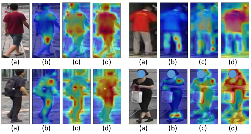
Figure 3: Visualization. (a) Input images, (b) TransReID baseline, (c) our baseline (d) CLIP-ReID.

Conclusion

This paper investigates the way to apply the vision-language pre-training model in image ReID. We find that fine-tuning the visual model initialized by the CLIP image encoder, either ResNet-50 or ViT-B/16, gives a good performance compared to other baselines. To fully utilize the cross-modal description ability in the pre-trained model, we propose CLIP-ReID with a two-stage training strategy, in which the learnable text tokens shared within each ID are incorporated and augmented to describe different instances. In the first stage, only these tokens get optimized, forming ambiguous text descriptions. In the second stage, these tokens and text encoder together provide constraints for optimizing the parameters in the image encoder. We validate CLIP-ReID on several datasets of persons and vehicles, and the results demonstrate the effectiveness of text descriptions and the superiority of our model.

Appendix A Supplementary Material

Alternative way for the first training stage.

In order to improve the training efficiency in the first stage, we propose another method, which computes the $\mathcal{L}_{t2ice}$ based on the average image feature $V_{y_{i}}$ among all images with ID $y_{i}$. Since the image encoder keeps fixed, $V_{y_{i}}$ can be computed offline, and buffered in the memory. In this way, the first stage is completed in a short time at the expense of final performance dropping, shown in Tab. 8.

$$\mathcal{L}_{t2ice}(y_{i})=-\log\frac{\exp(s(V_{y_{i}},T_{y_{i}}))}{\sum_{{y_{a}}=1}^{N}\exp(s(V_{y_{a}},T_{y_{i}}))}$$ (10)

Methods	MSMT17			Market-1501
	mAP	R1	T	mAP	R1	T
average	72.4	88.3	2.0	89.3	95.2	2.0
instance	73.4	88.6	37.5	89.6	95.5	15.5

Table 8: Comparison between two training methods in the first stage. T denotes the time of training in minutes. We implement ViT-based model on a single NVIDIA GeForce RTX 2080 Ti GPU.

Retrieval result visualization.

We visualize the retrieval results on MSMT17, with the incorrectly identified samples highlighted in orange.

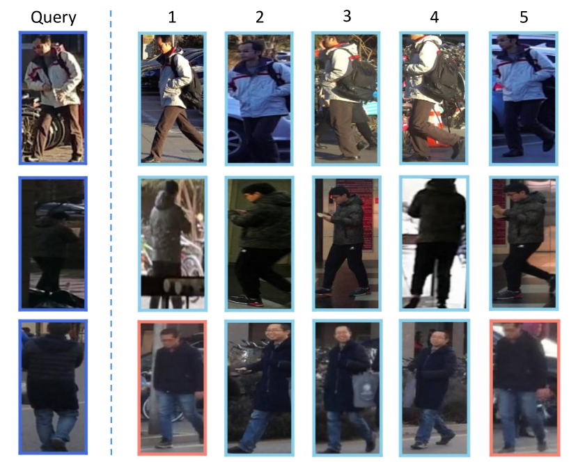
Figure 4: Retrieval result visualization.

The $\mathcal{L}_{tri}$ of the previous layer.

We find that adding $\mathcal{L}_{tri}$ to the previous layer usually improves the model’s ability to discriminate between different IDs, as shown in Tab. 9. Therefore, we employ $\mathcal{L}_{tri}$ after the 11th transformer layer of ViT-B/16 and the 3rd residual layer of ResNet-50. To give a clear illustration of our loss constraint, we show them in the CNN version of CLIP-ReID in Fig. 5.

Back- bone	Methods	MSMT17
		mAP	R1
CNN	baseline wo pre $\mathcal{L}_{tri}$	57.7	79.8
	baseline	60.7	82.1
	CLIP-ReID wo pre $\mathcal{L}_{tri}$	59.5	82.1
	CLIP-ReID	63.0	84.4
ViT	baseline wo pre $\mathcal{L}_{tri}$	65.9	84.2
	baseline	66.0	84.4
	CLIP-ReID wo pre $\mathcal{L}_{tri}$	73.1	88.6
	CLIP-ReID	73.4	88.7

Table 9: Comparison of w/wo $\mathcal{L}_{tri}$ of the previous layer.

Number of learnable tokens M.

We conduct analysis on the number of learnable tokens $\rm M$ in Tab. 10. It shows that the performance is not sensitive to $\rm M$, and $\rm M=4$ gives the best results, as we present in the manuscript.

$\rm M$	MSMT17		Market-1501
	mAP	R1	mAP	R1
1	72.7	88.4	89.5	94.9
4	73.4	88.7	89.6	95.5
8	73.4	88.6	89.5	95.1

Table 10: Performance analysis on parameter $\rm M$ for ViT-based.

Dimensions of inference features

As shown in Fig. 5, we have three image features to use during inference, the results of different combinations in Tab. 11. We concatenate the img_feature and post_img_feature as the final feature representation.

Comparison with state-of-the-art methods on two vehicle datasets.

We further intensively evaluate our proposed method on two vehicle ReID datasets, and the full metrics are shown in Tab. 12. For the VehicleID dataset, the test sets are available in small, medium, and large versions, and CLIP-ReID achieves promising results in all the three settings.

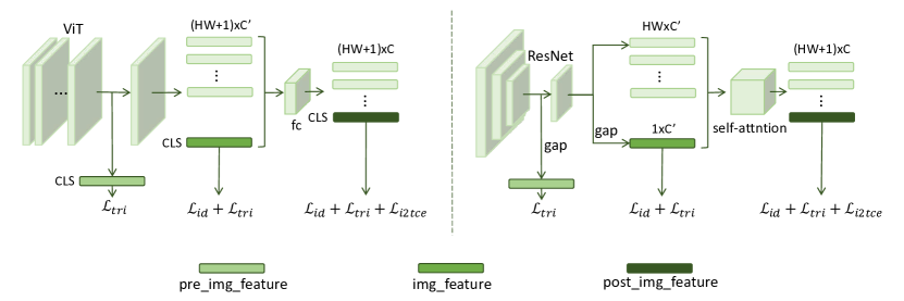
Figure 5: Details of the CNN-based CLIP-ReID image encoder.

Backbone	Inference features	Dim	MSMT17		Market-1501
			mAP	R1	mAP	R1
CNN	post_img_feature	1024	61.3	84.0	88.6	95.2
	pre_img_feature	2048	48.3	68.8	83.1	91.9
	img_feature	2048	57.6	80.5	88.6	95.2
	img_feature + post_img_feature	3072	63.0	84.4	89.8	95.7
	img_feature + pre_img_feature	4096	57.0	78.7	88.5	94.9
	pre_img_feature + img_feature + post_img_feature	5120	62.9	83.9	89.9	95.6
ViT	post_img_feature	512	72.3	88.2	89.0	94.9
	pre_img_feature	768	71.7	87.1	88.3	94.7
	img_feature	768	73.4	88.7	89.6	95.4
	img_feature + post_img_feature	1280	73.4	88.7	89.6	95.5
	img_feature + pre_img_feature	1536	73.6	88.6	89.7	95.5
	pre_img_feature + img_feature + post_img_feature	2048	73.6	88.6	89.7	95.5

Table 11: The validations on different inferece features.

Methods	VeRi-776			VehicleID
				Small			Medium			Large
	mAP	R1	R5	R1	R5	mAP	R1	R5	mAP	R1	R5	mAP
PRN	74.3	94.3	98.7	78.4	92.3	-	75.0	88.3	-	74.2	86.4	-
SAN	72.5	93.3	97.1	79.7	94.3	-	78.4	91.3		75.6	88.3
UMTS	75.9	95.8	-	80.9	-	87.0	78.8	-	84.2	76.1	-	82.8
PVEN	79.5	95.6	98.4	84.7	97.0	-	80.6	94.5	-	77.8	92.0	-
SAVER	79.6	96.4	98.6	79.9	95.2	-	77.6	91.1	-	75.3	88.3	-
CFVMNet	77.1	95.3	98.4	81.4	94.1	-	77.3	90.4	-	74.7	88.7	-
CAL	74.3	95.4	97.9	82.5	94.7	87.8	78.2	91.0	83.8	75.1	88.5	80.9
CLIP-ReID (CNN)	80.3	96.8	98.4	85.2	97.1	90.3	80.7	94.3	86.5	78.7	92.3	84.6
CLIP-ReID (ViT)	83.3	97.4	98.6	85.3	97.6	90.6	81.0	95.0	86.9	78.1	92.7	84.4

Table 12: Comparisons with the state-of-the-art vehicle ReID methods on the VeRi-776 and VehicleID datasets.

References

- Baldrati et al. (2022) Baldrati, A.; Bertini, M.; Uricchio, T.; and Del Bimbo, A. 2022. Effective Conditioned and Composed Image Retrieval Combining CLIP-Based Features. In Proceedings of the IEEE/CVF CVPR, 21466–21474.
- Chefer, Gur, and Wolf (2021) Chefer, H.; Gur, S.; and Wolf, L. 2021. Transformer interpretability beyond attention visualization. In Proceedings of the IEEE/CVF CVPR, 782–791.
- Chen et al. (2019) Chen, T.; Ding, S.; Xie, J.; Yuan, Y.; Chen, W.; Yang, Y.; Ren, Z.; and Wang, Z. 2019. Abd-net: Attentive but diverse person re-identification. In Proceedings of the IEEE/CVF international conference on computer vision, 8351–8361.
- Chen et al. (2020) Chen, T.-S.; Liu, C.-T.; Wu, C.-W.; and Chien, S.-Y. 2020. Orientation-aware vehicle re-identification with semantics-guided part attention network. In European conference on computer vision, 330–346. Springer.
- Dai et al. (2019) Dai, Z.; Chen, M.; Gu, X.; Zhu, S.; and Tan, P. 2019. Batch dropblock network for person re-identification and beyond. In Proceedings of the IEEE/CVF international conference on computer vision, 3691–3701.
- Das, Chakraborty, and Roy-Chowdhury (2014) Das, A.; Chakraborty, A.; and Roy-Chowdhury, A. K. 2014. Consistent re-identification in a camera network. In European conference on computer vision, 330–345. Springer.
- Dosovitskiy et al. (2020) Dosovitskiy, A.; Beyer, L.; Kolesnikov, A.; Weissenborn, D.; Zhai, X.; Unterthiner, T.; Dehghani, M.; Minderer, M.; Heigold, G.; Gelly, S.; et al. 2020. An image is worth 16x16 words: Transformers for image recognition at scale. arXiv preprint arXiv:2010.11929.
- Gao et al. (2021) Gao, P.; Geng, S.; Zhang, R.; Ma, T.; Fang, R.; Zhang, Y.; Li, H.; and Qiao, Y. 2021. Clip-adapter: Better vision-language models with feature adapters. arXiv preprint arXiv:2110.04544.
- Gu et al. (2021) Gu, X.; Lin, T.-Y.; Kuo, W.; and Cui, Y. 2021. Open-vocabulary object detection via vision and language knowledge distillation. arXiv preprint arXiv:2104.13921.
- He et al. (2019) He, B.; Li, J.; Zhao, Y.; and Tian, Y. 2019. Part-regularized near-duplicate vehicle re-identification. In Proceedings of the IEEE/CVF CVPR, 3997–4005.
- He et al. (2016) He, K.; Zhang, X.; Ren, S.; and Sun, J. 2016. Deep residual learning for image recognition. In Proceedings of the IEEE Conference on Computer Vision and Pattern Recognition (CVPR), 770–778.
- He et al. (2021) He, S.; Luo, H.; Wang, P.; Wang, F.; Li, H.; and Jiang, W. 2021. Transreid: Transformer-based object re-identification. In Proceedings of the IEEE/CVF international conference on computer vision, 15013–15022.
- Hermans, Beyer, and Leibe (2017) Hermans, A.; Beyer, L.; and Leibe, B. 2017. In defense of the triplet loss for person re-identification. arXiv preprint arXiv:1703.07737.
- Jia et al. (2021) Jia, C.; Yang, Y.; Xia, Y.; Chen, Y.-T.; Parekh, Z.; Pham, H.; Le, Q.; Sung, Y.-H.; Li, Z.; and Duerig, T. 2021. Scaling up visual and vision-language representation learning with noisy text supervision. In International Conference on Machine Learning, 4904–4916. PMLR.
- Jia et al. (2022) Jia, M.; Cheng, X.; Lu, S.; and Zhang, J. 2022. Learning disentangled representation implicitly via transformer for occluded person re-identification. IEEE Transactions on Multimedia.
- Jin et al. (2020a) Jin, X.; Lan, C.; Zeng, W.; and Chen, Z. 2020a. Uncertainty-aware multi-shot knowledge distillation for image-based object re-identification. In Proceedings of the AAAI Conference on Artificial Intelligence, volume 34, 11165–11172.
- Jin et al. (2020b) Jin, X.; Lan, C.; Zeng, W.; Wei, G.; and Chen, Z. 2020b. Semantics-aligned representation learning for person re-identification. In Proceedings of the AAAI Conference on Artificial Intelligence, volume 34, 11173–11180.
- Khorramshahi et al. (2020) Khorramshahi, P.; Peri, N.; Chen, J.-c.; and Chellappa, R. 2020. The devil is in the details: Self-supervised attention for vehicle re-identification. In European Conference on Computer Vision, 369–386. Springer.
- Kim, Son, and Kim (2021) Kim, W.; Son, B.; and Kim, I. 2021. Vilt: Vision-and-language transformer without convolution or region supervision. In International Conference on Machine Learning, 5583–5594. PMLR.
- Koestinger et al. (2012) Koestinger, M.; Hirzer, M.; Wohlhart, P.; Roth, P. M.; and Bischof, H. 2012. Large scale metric learning from equivalence constraints. In 2012 IEEE CVPR, 2288–2295. IEEE.
- Li, Wu, and Zheng (2021) Li, H.; Wu, G.; and Zheng, W.-S. 2021. Combined depth space based architecture search for person re-identification. In Proceedings of the IEEE/CVF CVPR, 6729–6738.
- Li et al. (2022) Li, J.; Li, D.; Xiong, C.; and Hoi, S. 2022. Blip: Bootstrapping language-image pre-training for unified vision-language understanding and generation. arXiv preprint arXiv:2201.12086.
- Li et al. (2021a) Li, J.; Selvaraju, R.; Gotmare, A.; Joty, S.; Xiong, C.; and Hoi, S. C. H. 2021a. Align before fuse: Vision and language representation learning with momentum distillation. Advances in neural information processing systems, 34: 9694–9705.
- Li et al. (2021b) Li, Y.; He, J.; Zhang, T.; Liu, X.; Zhang, Y.; and Wu, F. 2021b. Diverse part discovery: Occluded person re-identification with part-aware transformer. In Proceedings of the IEEE/CVF CVPR, 2898–2907.
- Liang et al. (2018) Liang, L.; Lang, C.; Li, Z.; Zhao, J.; Wang, T.; and Feng, S. 2018. Seeing Crucial Parts: Vehicle Model Verification via A Discriminative Representation Model. Journal of the ACM (JACM), 22.
- Liao et al. (2015) Liao, S.; Hu, Y.; Zhu, X.; and Li, S. Z. 2015. Person re-identification by local maximal occurrence representation and metric learning. In Proceedings of the IEEE CVPR, 2197–2206.
- Liu et al. (2016a) Liu, H.; Tian, Y.; Yang, Y.; Pang, L.; and Huang, T. 2016a. Deep relative distance learning: Tell the difference between similar vehicles. In Proceedings of the IEEE CVPR, 2167–2175.
- Liu et al. (2016b) Liu, X.; Liu, W.; Ma, H.; and Fu, H. 2016b. Large-scale vehicle re-identification in urban surveillance videos. In 2016 IEEE international conference on multimedia and expo (ICME), 1–6. IEEE.
- Luo et al. (2019) Luo, H.; Gu, Y.; Liao, X.; Lai, S.; and Jiang, W. 2019. Bag of tricks and a strong baseline for deep person re-identification. In Proceedings of the IEEE/CVF CVPR workshops, 0–0.
- Ma et al. (2022) Ma, H.; Zhao, H.; Lin, Z.; Kale, A.; Wang, Z.; Yu, T.; Gu, J.; Choudhary, S.; and Xie, X. 2022. EI-CLIP: Entity-Aware Interventional Contrastive Learning for E-Commerce Cross-Modal Retrieval. In Proceedings of the IEEE/CVF CVPR, 18051–18061.
- Matsukawa et al. (2016) Matsukawa, T.; Okabe, T.; Suzuki, E.; and Sato, Y. 2016. Hierarchical gaussian descriptor for person re-identification. In Proceedings of the IEEE CVPR, 1363–1372.
- Meng et al. (2020) Meng, D.; Li, L.; Liu, X.; Li, Y.; Yang, S.; Zha, Z.-J.; Gao, X.; Wang, S.; and Huang, Q. 2020. Parsing-based view-aware embedding network for vehicle re-identification. In Proceedings of the IEEE/CVF CVPR, 7103–7112.
- Miao et al. (2019) Miao, J.; Wu, Y.; Liu, P.; Ding, Y.; and Yang, Y. 2019. Pose-guided feature alignment for occluded person re-identification. In Proceedings of the IEEE/CVF international conference on computer vision, 542–551.
- Qian et al. (2020) Qian, J.; Jiang, W.; Luo, H.; and Yu, H. 2020. Stripe-based and attribute-aware network: A two-branch deep model for vehicle re-identification. Measurement Science and Technology, 31(9): 095401.
- Quan et al. (2019) Quan, R.; Dong, X.; Wu, Y.; Zhu, L.; and Yang, Y. 2019. Auto-reid: Searching for a part-aware convnet for person re-identification. In Proceedings of the IEEE/CVF International Conference on Computer Vision, 3750–3759.
- Radford et al. (2021) Radford, A.; Kim, J. W.; Hallacy, C.; Ramesh, A.; Goh, G.; Agarwal, S.; Sastry, G.; Askell, A.; Mishkin, P.; Clark, J.; et al. 2021. Learning transferable visual models from natural language supervision. In International Conference on Machine Learning, 8748–8763. PMLR.
- Rao et al. (2021) Rao, Y.; Chen, G.; Lu, J.; and Zhou, J. 2021. Counterfactual attention learning for fine-grained visual categorization and re-identification. In Proceedings of the IEEE/CVF International Conference on Computer Vision, 1025–1034.
- Rao et al. (2022) Rao, Y.; Zhao, W.; Chen, G.; Tang, Y.; Zhu, Z.; Huang, G.; Zhou, J.; and Lu, J. 2022. Denseclip: Language-guided dense prediction with context-aware prompting. In Proceedings of the IEEE/CVF CVPR, 18082–18091.
- Ristani et al. (2016) Ristani, E.; Solera, F.; Zou, R.; Cucchiara, R.; and Tomasi, C. 2016. Performance measures and a data set for multi-target, multi-camera tracking. In European conference on computer vision, 17–35. Springer.
- Sennrich, Haddow, and Birch (2015) Sennrich, R.; Haddow, B.; and Birch, A. 2015. Neural machine translation of rare words with subword units. arXiv preprint arXiv:1508.07909.
- Sun et al. (2018) Sun, Y.; Zheng, L.; Yang, Y.; Tian, Q.; and Wang, S. 2018. Beyond part models: Person retrieval with refined part pooling (and a strong convolutional baseline). In Proceedings of the European conference on computer vision (ECCV), 480–496.
- Sun et al. (2020) Sun, Z.; Nie, X.; Xi, X.; and Yin, Y. 2020. Cfvmnet: A multi-branch network for vehicle re-identification based on common field of view. In Proceedings of the 28th ACM international conference on multimedia, 3523–3531.
- Tan et al. (2021) Tan, H.; Liu, X.; Bian, Y.; Wang, H.; and Yin, B. 2021. Incomplete descriptor mining with elastic loss for person re-identification. IEEE Transactions on Circuits and Systems for Video Technology, 32(1): 160–171.
- Van der Maaten and Hinton (2008) Van der Maaten, L.; and Hinton, G. 2008. Visualizing data using t-SNE. Journal of machine learning research, 9(11).
- Wang et al. (2020) Wang, G.; Yang, S.; Liu, H.; Wang, Z.; Yang, Y.; Wang, S.; Yu, G.; Zhou, E.; and Sun, J. 2020. High-order information matters: Learning relation and topology for occluded person re-identification. In Proceedings of the IEEE/CVF CVPR, 6449–6458.
- Wang et al. (2018) Wang, G.; Yuan, Y.; Chen, X.; Li, J.; and Zhou, X. 2018. Learning discriminative features with multiple granularities for person re-identification. In Proceedings of the 26th ACM international conference on Multimedia, 274–282.
- Wang et al. (2022) Wang, P.; Zhao, Z.; Su, F.; and Meng, H. 2022. LTReID: Factorizable Feature Generation with Independent Components for Long-Tailed Person Re-Identification. IEEE Transactions on Multimedia.
- Wang et al. (2021) Wang, Z.; Yu, J.; Yu, A. W.; Dai, Z.; Tsvetkov, Y.; and Cao, Y. 2021. Simvlm: Simple visual language model pretraining with weak supervision. arXiv preprint arXiv:2108.10904.
- Wei et al. (2018) Wei, L.; Zhang, S.; Gao, W.; and Tian, Q. 2018. Person transfer gan to bridge domain gap for person re-identification. In Proceedings of the IEEE CVPR, 79–88.
- Yan et al. (2021) Yan, C.; Pang, G.; Bai, X.; Liu, C.; Ning, X.; Gu, L.; and Zhou, J. 2021. Beyond triplet loss: person re-identification with fine-grained difference-aware pairwise loss. IEEE Transactions on Multimedia, 24: 1665–1677.
- Yi et al. (2014) Yi, D.; Lei, Z.; Liao, S.; and Li, S. Z. 2014. Deep metric learning for person re-identification. In 2014 22nd international conference on pattern recognition, 34–39. IEEE.
- Zhang et al. (2021a) Zhang, E.; Jiang, X.; Cheng, H.; Wu, A.; Yu, F.; Li, K.; Guo, X.; Zheng, F.; Zheng, W.; and Sun, X. 2021a. One for More: Selecting Generalizable Samples for Generalizable ReID Model. In Proceedings of the AAAI Conference on Artificial Intelligence, volume 35, 3324–3332.
- Zhang et al. (2021b) Zhang, Q.; Lai, J.; Feng, Z.; and Xie, X. 2021b. Seeing like a human: Asynchronous learning with dynamic progressive refinement for person re-identification. IEEE Transactions on Image Processing, 31: 352–365.
- Zhang et al. (2019) Zhang, X.; Zhang, R.; Cao, J.; Gong, D.; You, M.; and Shen, C. 2019. Part-guided attention learning for vehicle re-identification. arXiv preprint arXiv:1909.06023, 2(8).
- Zhang et al. (2021c) Zhang, Y.; He, B.; Sun, L.; and Li, Q. 2021c. Progressive Multi-Stage Feature Mix for Person Re-Identification. In ICASSP 2021-2021 IEEE International Conference on Acoustics, Speech and Signal Processing (ICASSP), 2765–2769. IEEE.
- Zhang et al. (2020) Zhang, Z.; Lan, C.; Zeng, W.; Jin, X.; and Chen, Z. 2020. Relation-aware global attention for person re-identification. In Proceedings of the ieee/cvf CVPR, 3186–3195.
- Zheng et al. (2015) Zheng, L.; Shen, L.; Tian, L.; Wang, S.; Wang, J.; and Tian, Q. 2015. Scalable person re-identification: A benchmark. In Proceedings of the IEEE international conference on computer vision, 1116–1124.
- Zhong et al. (2020) Zhong, Z.; Zheng, L.; Kang, G.; Li, S.; and Yang, Y. 2020. Random erasing data augmentation. In Proceedings of the AAAI conference on artificial intelligence, volume 34, 13001–13008.
- Zhou, Loy, and Dai (2021) Zhou, C.; Loy, C. C.; and Dai, B. 2021. Denseclip: Extract free dense labels from clip. arXiv preprint arXiv:2112.01071.
- Zhou et al. (2021) Zhou, K.; Yang, J.; Loy, C. C.; and Liu, Z. 2021. Learning to Prompt for Vision-Language Models.
- Zhou et al. (2022) Zhou, K.; Yang, J.; Loy, C. C.; and Liu, Z. 2022. Conditional prompt learning for vision-language models. In Proceedings of the IEEE/CVF CVPR, 16816–16825.
- Zhou et al. (2019) Zhou, K.; Yang, Y.; Cavallaro, A.; and Xiang, T. 2019. Omni-scale feature learning for person re-identification. In Proceedings of the IEEE/CVF International Conference on Computer Vision, 3702–3712.
- Zhu et al. (2022) Zhu, H.; Ke, W.; Li, D.; Liu, J.; Tian, L.; and Shan, Y. 2022. Dual Cross-Attention Learning for Fine-Grained Visual Categorization and Object Re-Identification. In Proceedings of the IEEE/CVF CVPR, 4692–4702.
- Zhu et al. (2020) Zhu, K.; Guo, H.; Liu, Z.; Tang, M.; and Wang, J. 2020. Identity-guided human semantic parsing for person re-identification. In European Conference on Computer Vision, 346–363. Springer.
- Zhu et al. (2021) Zhu, K.; Guo, H.; Zhang, S.; Wang, Y.; Huang, G.; Qiao, H.; Liu, J.; Wang, J.; and Tang, M. 2021. Aaformer: Auto-aligned transformer for person re-identification. arXiv preprint arXiv:2104.00921.