Probability Distribution Functions of Sunspot Magnetic Flux

Abstract

We have investigated the probability distributions of sunspot area and magnetic flux by using the data from Royal Greenwich Observatory and USAF/NOAA. We have constructed a sample of 2995 regions with maximum-development areas $\geq$ 500 MSH (millionths of solar hemisphere), covering 146.7 years (1874–2020). The data were fitted by a power-law distribution and four two-parameter distributions (tapered power-law, gamma, lognormal, and Weibull distributions). The power-law model was unfavorable compared to the four models in terms of AIC, and was not acceptable by the classical Kolmogorov-Smirnov test. The lognormal and Weibull distributions were excluded because their behavior extended to smaller regions ($S\ll 500$ MSH) do not connect to the previously published results. Therefore, our choices were tapered power-law and gamma distributions. The power-law portion of the tapered power-law and gamma distributions was found to have a power exponent of 1.35–1.9. Due to the exponential fall-off of these distributions, the expected frequencies of large sunspots are low. The largest sunspot group observed had an area of 6132 MSH, and the frequency of sunspots larger than $10^{4}$ MSH was estimated to be every 3 – 8 $\times 10^{4}$ years. We also have estimated the distributions of the Sun-as-a-star total sunspot areas. The largest total area covered by sunspots in the record was 1.67 % of the visible disk, and can be up to 2.7 % by artificially increasing the lifetimes of large sunspots in an area evolution model. These values are still smaller than those found on active Sun-like stars.

1 Introduction

Sunspots represent a variety of magnetic activities of the Sun (sol03; van15). It is thought that the dynamo mechanism in the solar interior intensifies and transports magnetic flux to the surface and eventually builds up active regions (ARs) including sunspots (par55). Even after four centuries of continuous observations, the sunspots still maintain important positions in the investigation of the dynamo processes in the Sun.

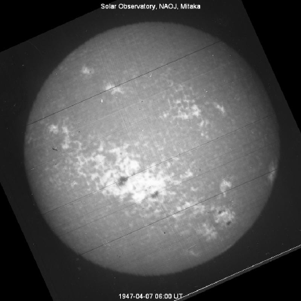
Figure 1: Ca K-line spectroheliogram of 1947 April 7 taken at Mitaka, Tokyo; celestial north is up, west to the right. The big active region near the disk center is RGO region 14886 which showed a foreshortening-corrected area of 6132 MSH, the largest on the record, on April 8.

Another importance of sunspots is their close relationship with flare activity (pri02; shi11; tor19). Statistical investigations have revealed that greater flares emanate from larger ARs (sam00). This may be natural since larger ARs harbor more magnetic flux and thus more magnetic free energy available. The largest observed sunspot group since the late nineteenth century was the one in 1947 April, the largest area of which was 6132 MSH (millionths of solar hemisphere; 1 MSH = $3.04\times 10^{6}$ km${}^{2}$) or about 1.2 % of the visible solar disk (Figure 1). While this region was not flare-active, another giant sunspot in 1946 July caused larger flares with geomagnetic disturbances (tor17). The formation mechanism of such great ARs is an interesting issue to be resolved.

The existence of spots is also known for other stars (ber05; str09). One of the largest starspots reported thus far was from a K0 giant XX Tri (HD 12545), which covered about 20% of the entire stellar surface (str99). It was found that even solar-type stars producing the so-called superflares (sch00; mae12) host starspots much larger than the solar ones (up to $\sim 10\%$ of the stellar hemisphere; not13; not15). Therefore, the discussion of superflares on the Sun is closely related to the question of the production of super-large sunspots.

The key quantity we study in this paper is the probability distribution function of the area $S$ or magnetic flux $\Phi$ of sunspots. bog88 analyzed the Mt. Wilson white-light observations (1917–1982) of sunspots and showed that the sunspot umbral areas [1.5–141 MSH; the corresponding total sunspot areas would be about five times of these (sol03)] follow the lognormal distribution. hat08 obtained the same conclusion using the data from the Royal Greenwich Observatory (RGO) and the United States Air Force [USAF; data were compiled and distributed by the National Oceanic and Atmospheric Administration (NOAA)] covering the period 1874–2007 (sunspot areas larger than 35 MSH). bau05 studied the RGO data (1874–1976) of sunspots with areas $\geq 60$ MSH, by making a distinction between a snapshot distribution and a maximum area distribution; the former is derived from daily data (e.g. bog88; hat08) while the latter is derived by following the time evolution of individual regions and by recording their maximum areas. They found that the two distributions are fitted by lognormal distributions that have similar parameter values. This property was also mentioned in hat08.

The fall-off of the lognormal distribution toward small sunspot areas may be because smaller magnetic concentrations tend to lose their darkness and eventually end up with small flux tubes brighter than the surroundings (zwa87). On the other hand, the fall-off of the lognormal distribution toward large sunspot areas was not paid much attention. In this context, gop18 applied the Weibull distribution (wei39), which is often used to describe the failure rates of industrial products, to the RGO and USAF/NOAA sunspot area data (maximum-area distribution). The tail of the observed distribution was fitted equally well by a power law and Weibull, and the latter gives more rapid decline and less frequent appearance of extremely large regions.

Since sunspots are made (i.e. obtain their darkness) because of their magnetic fields by inhibition of convective heat transport (e.g. spr77), the probability distribution of magnetic flux in magnetic structures (including sunspots) is an equally important quantity. khz93 analyzed the magnetograms obtained at the US National Solar Observatory at Kitt Peak (NSO/Kitt Peak) in the period 1975–1986 and derived the distribution of magnetic flux at the maximum development of individual active regions. For regions with areas larger than 121 MSH the magnetic flux emergence rate was approximated by a power law. sch94 gave a more specific fitting equation with a power-law exponent of about 2.0 [probability $\propto\Phi^{-\alpha}$ with $\alpha\simeq 2$; in this article $\alpha(>0)$ is called the power-law exponent]. hst03 investigated the emergence rates of ephemeral regions (small-scale bipolar magnetic field patches) using the data from the Michelson Doppler Imager onboard the Solar and Heliospheric Observatory (SOHO/MDI; sch95) taken between 1996 and 2001. They found that the distribution looked like an exponential function. tho11 analyzed the emergence rates of small-scale magnetic field patches using the data from the Solar Optical Telescope onboard the Hinode satellite (Hinode/SOT; tsu08) and obtained a power-law formula extending all the way up to the active-region scales, with a power-law exponent of 2.69. All of these results are summarized and discussed later in Section 5 and in Figure 7. bal09, mun15, and man20 give detailed accounts on the issues on sunspot area calibration. mun15 also tried several models (power law, lognormal, Weibul, exponential, and their combinations) to fit the area distributions.

In this paper, we will use the data from RGO (1874–1976) and USAF/NOAA (1977 - 2020) and derive the maximum areas of individual regions (Section 2). Recurrent regions are counted only once when their areas reach the maximum. In order to compare these with magnetic field observations of active regions and smaller magnetic patches, we will convert the sunspot areas to magnetic flux values (Section 2.2). Our primary interest here is whether the sunspot area or magnetic flux distribution extends to large values in the form of a power law or is tapered off, to address whether the Sun may have super-large sunspots like in super-flare stars. Therefore, we limit the data of sunspots with areas 500 MSH or larger, and try to fit the data with five kinds of distribution functions; power law, tapered power law, gamma, lognormal, and Weibull distributions (Section 3). Statistical examinations (Section 4) and comparison with previously published results (Section 5) show preference on the tapered power law and gamma distributions. Using the obtained results, we can predict the expected frequencies of super-large sunspots. In Section 6, we will adopt a simple time-evolution model of sunspot areas and examine the effects of assumptions we made in our analysis. Particularly we can estimate the snapshot (instantaneous) distribution of sunspot areas (Section LABEL:sec:instantaneous) and also a distribution of Sun-as-a-star total sunspot areas (Section LABEL:sec:whole-Sun), and will discuss their implications on super-large stellar spots (Section LABEL:sec:summary).

2 Data

2.1 Data Sources

The Greenwich Photoheliographic Results (GPR) in PDF are available through the SAO/NASA Astrophysics Data System (ADS), NOAA, and the UK Solar System Data Center. The digitized data of sunspot areas recorded in GPR (1874 April – 1976) are provided at several sites${}^{,}$${}^{,}$. Systematic observation and data collection of sunspots at RGO started on 1874 April 17 (chr1907). The correction for foreshortening was explained to have been applied to regions of angular distance within $80^{\circ}$ from the disk center (rgo55), but regions beyond were occasionally recorded. From these data sets we have picked up regions whose foreshortening-corrected maximum-development areas ($S_{\rm md}$) are 500 MSH or larger. If the corrected area $S$ of a region was monotonically increasing or decreasing on the visible hemisphere, we defined the maximum value of $S$ as the maximum-development area $S_{\rm md}$, although the true maximum took place on the back-side of the Sun. The effects of this assumption will be estimated in Section 6. For recurrent regions, we only retained the maximum $S$ over all their disk passages because they were regarded as generated from the identical magnetic flux tubes generated by the dynamo. For this we had to identify recurrent regions, and such lists are available in mau1909 (1874–1906), and “Catalogue of Recurrent Groups of Sun Spots” (1910–1955), “Ledger I: Recurrent Groups” (1916–1955), and “General Catalog of Groups of Sunspots” (1956–1976) sections of GPR.

The data after the cessation of RGO solar observations in 1976 were taken from USAF/NOAA (1977–2020)${}^{5}$. As no convenient lists are available to identify recurrent regions, we did this manually by relying on the following data: H$\alpha$ synoptic charts in Solar Geophysical Data (SGD) (1977–1989), NOAA Report of Solar and Geophysical Activity (RSGA) (1990–2000), NOAA Weekly Preliminary Report and Forecast of SGD (Weekly PRF)${}^{7}$ (2001–2009), and Debrecen Photoheliographic Data (DPD) (2010–2020). We have picked up regions with the foreshortening-corrected maximum-development area exceeding 500/1.20 = 415 MSH (see below). The distribution of angular distances from the disk center did not show a clear decline toward the limb and continued up to $90^{\circ}$, implying that the foreshortening correction was applied to all the USAF/NOAA data.

In the end we have selected 2995 regions, 2175 from RGO and 820 from USAF/NOAA data, covering 1874 April to 2020 December, 146.7 years (Table 1). Before obtaining the final list, we have removed 363 and 101 regions from RGO and USAF/NOAA data as they were members of recurrent regions. The data fully cover 13 solar cycles, from Cycle 12 (1878 December – 1890 March) to Cycle 24 (2008 December – 2019 December).

Table 1: Data

No.	Date	Data source	Region number	RGO area	Original area${}^{a}$	Magnetic flux
				[MSH]	[MSH]	[Mx]
1	1947-04-08	RGO	14886	6132.0	6132	3.18E+23
2	1946-02-07	RGO	14417	5202.0	5202	2.69E+23
3	1951-05-19	RGO	16763	4865.0	4865	2.51E+23
4	1946-07-29	RGO	14585	4720.0	4720	2.44E+23
5	1989-03-18	NOAA	5395	4320.0	3600	2.23E+23
6	1982-06-15	NOAA	3776	3720.0	3100	1.92E+23
7	1926-01-19	RGO	9861	3716.0	3716	1.92E+23
8	1989-09-04	NOAA	5669	3696.0	3080	1.91E+23
9	1990-11-19	NOAA	6368	3696.0	3080	1.91E+23
10	1938-01-21	RGO	12673	3627.0	3627	1.87e+23
${}^{a}$: NOAA area before converted to the RGO scale.

2.2 Sunspot Area vs. Magnetic Flux

In order to relate the sunspot area and the total radial unsigned magnetic flux (including the flux outside of the sunspots), we used the SHARP data series (bob14) of the Helioseismic and Magnetic Imager (HMI; sche12; scho12) aboard the Solar Dynamics Observatory (SDO; pes12). We picked up all available CEA (cylindrical equal area)-remapped definitive SHARP data from 2010 to 2015 that contained the sunspots of NOAA areas $\geq 500\ {\rm MSH}$ within 45${}^{\circ}$ from the disk center. In total, 137 patches were collected (one patch per region per day). From each patch, we carefully eliminated magnetic concentrations that were not related to the target ARs.

In order to evaluate the total unsigned magnetic flux in maxwell (Mx) from the list of the sunspot areas, we investigated the relation between the sunspot area, $S_{\rm HMI}$, and the total unsigned radial flux, $\Phi_{\rm HMI}$, which can also be calculated from the SHARP data. Note that we measured the total flux only within the smooth bounding curve of the SHARP data to minimize the possibility of including flux that was not related to the target AR and to reduce the noise effect. Figure 2(a) shows a scatter plot between $S_{\rm HMI}$ and $\Phi_{\rm HMI}$. From the least-squares fitting to this double logarithmic plot, we obtained the relation between the two parameters,

$$\log{(\Phi_{\rm HMI}\ {\rm[Mx]})} = (1.010\pm 0.132)\times\log{(S_{\rm HMI}\ {\rm[MSH]})}$$ (1)

$$+ (19.676\pm 0.400),$$

($\log$ means $\log_{10}$; for natural logarithm we use “$\ln$” in this paper) where we assumed that both $\Phi_{\rm HMI}$ and $S_{\rm HMI}$ have errors (dem43; pre92). The obtained conversion equation shows that the total flux is almost linearly related to the sunspot area, $\Phi/S\simeq$ 1660 gauss (AR flux/sunspot area for $S\simeq$ 500 MSH). For comparison, sch94 derived AR flux/AR area $\simeq$ 150 gauss.

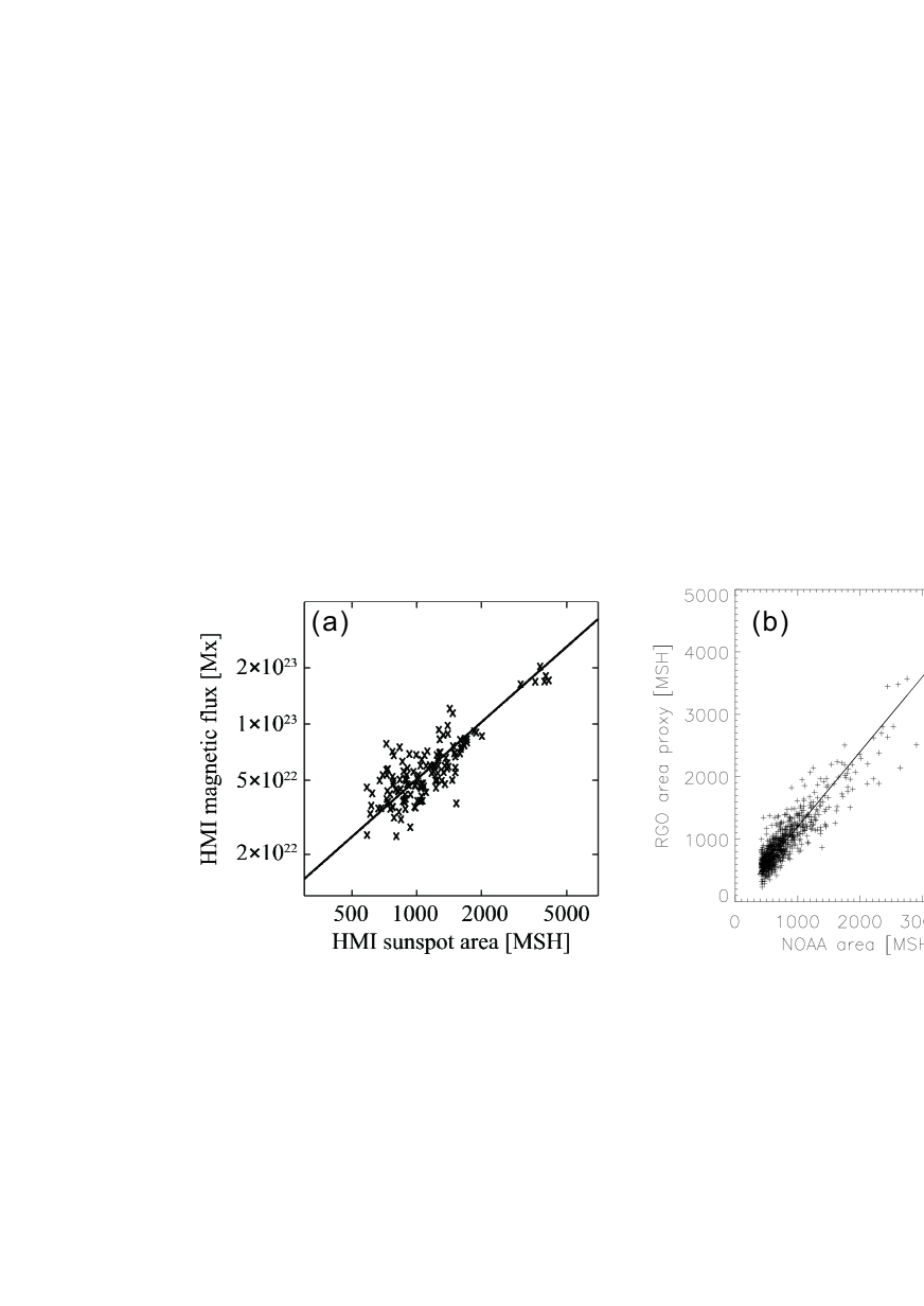
Figure 2: (a) Scatter plot between sunspot areas and total unsigned magnetic fluxes in ARs, both taken from the SHARP data, with the linear fitting to the log-log plot: see Equation (1). (b) Comparison of sunspot areas reported by NOAA vs. the database of man20 that reproduces the RGO area scale. The number of samples is 762. The solid line shows the regression line [Equation (2)]

2.3 Sunspot Area Calibration

It is known that the USAF/NOAA sunspot areas, $S_{\rm NOAA}$, are systematically smaller than the RGO ones, $S_{\rm RGO}$. In general, the multiplication of the USAF/NOAA values by 1.4–1.5 gives better agreement with the RGO values (e.g., fli97; hat02; bal09; hat15). However, fou14 showed that the inconsistency between the RGO and USAF/NOAA data sets was mainly due to very small sunspots ($\lesssim 2$ MSH) and that the areas for $>300$ MSH equalized. In order to examine if the NOAA records of larger ARs show systematically smaller values, we used the database developed by man20 which was calibrated to give the same area scale as RGO and was extended to 2021. Among our 820 NOAA regions we excluded 58 regions which we suspect that NOAA and man20 used different group definitions.

Figure 2(b) shows the comparison of 762 regions. We found that mean and standard deviation of the area ratios, $S_{\rm RGO}/S_{\rm NOAA}$, are 1.20 $\pm$ 0.01. Therefore, we simply assumed that the RGO data sets provide reliable values and the NOAA values are converted by

$$S=S_{\rm HMI}=S_{\rm RGO}=1.20\times S_{\rm NOAA}.$$ (2)

man20 obtained the conversion factor of 1.48, but the method of comparison is different; they compared daily data while our data are region-wise, maximum-development areas. We have also made the analysis adopting a conversion factor of about 1.4 and found basically the same results, although detailed numerical values changed.

Under the assumption of Equation (2), we then applied Equation (1) to the maximum-development sunspot areas $S_{\rm md}$ of both RGO and USAF/NOAA to generate the database on the maximum-development magnetic flux $\Phi_{\rm md}$. A 500 MSH sunspot corresponds to a magnetic flux of $2.53\times 10^{22}$ Mx. The largest sunspot so far, RGO 14886 in 1947 April (6132 MSH), is estimated to have a total flux of $3.18\times 10^{23}\ {\rm Mx}$. Flux estimations of modern events such as NOAA 9169, 9393, 10486, and 12192 showed good agreements with the independent measurements by, e.g., tia08, smy10, cri09, zha10, and sun15.

Figure 3: (a) The complimentary cumulative distribution function (CCDF) $F(\Phi)$ of magnetic flux $\Phi_{\rm md}$ [Mx] of large sunspot regions ($S_{\rm md}\geq 500\ {\rm MSH}$) at their maximum development, observed from 1874 April to the end of 2020 (146.7 years). The top horizontal axis shows the corresponding sunspot areas. The dotted curve represents the distribution when recurrent regions not at their maximum development are all counted. (b) A histogram representing the distribution function $f(\Phi_{\rm md})$ of emergence rates of magnetic flux $\Phi_{\rm md}$ of large sunspot regions, per bin width, unit area in Mm${}^{2}$, and day. The bin width is $\Delta\log\Phi_{\rm md}=0.125$. Vertical bars indicate the $\sqrt{N}$ uncertainty of $N$ regions contained in each bin (the last bin only contains two regions). The dotted histogram represents the distribution when recurrent regions not at their maximum development are all counted.

3 Statistical Analysis

3.1 Definitions

Our data are made of $N_{\rm s}$ = 2995 values of sunspot magnetic flux at their maximum development, $\Phi_{{\rm md},i}$ ($i=1,2,\ldots,N_{\rm s}$) (subscript “s” is meant for “sources” or “source flux tubes”). In the following we simply designate $\Phi_{\rm md}$ as $\Phi$ unless we have to distinguish between maximum-development values and other cases. The minimum value of $\Phi_{i}$’s is $\Phi_{1}=2.53\times 10^{22}$ Mx, corresponding to an area of 500 MSH. As a histogram representation of data depends on how one defines the data bins (cla09), we will work on the complementary cumulative distribution function [CCDF, represented by $F(\Phi)$] shown in Figure 3a, which is uniquely defined in terms of a given observational data set [Equation (LABEL:eq:CCDF_obs)]. CCDF is a decreasing function of its argument while the cumulative distribution function (CDF) is an increasing function; therefore, the usage of CCDF is intuitively more straightforward in comparing with the probability distribution function that is also a decreasing function of its argument in the present case.

The slope (or derivative) of CCDF is the usual probability distribution function [PDF, represented by $P(\Phi)$], but here we introduce dimensional parameters and define the flux emergence rate $f(\Phi)$ in units of regions Mx${}^{-1}{\rm Mm}^{-2}{\rm d}^{-1}$ as (Figure 3b)

$$f(\Phi)=P(\Phi)\frac{N_{\rm s}}{AT},\quad P(\Phi)=-\frac{{\rm d}F(\Phi)}{{\rm d}\Phi},$$ (3)

where $A$ stands for the area of observation (the full Sun, e.g. $6.2\times 10^{6}\ {\rm Mm}^{2}$ in Sections 4 and 5 and the hemisphere in Sections LABEL:sec:instantaneous) and $T$ =146.7 years $=5.36\times 10^{4}$ days. A histogram is generated showing $f(\Phi_{j})=N_{j}/(AT\Delta\Phi_{j})$, where $j$ stands for the bin number, and $N_{j}$ is the number of sunspot groups with flux values ranging from $\Phi_{j}$ to $\Phi_{j}+\Delta\Phi_{j}$. The flux bins are taken equi-distant in $\log\Phi$ ($\Delta\log\Phi=$ constant = 0.125), so that $\Delta\Phi_{j}=\Phi_{j}\ln(10)\Delta(\log\Phi_{j})$. The quantity $N_{\rm s}=\Sigma_{j}N_{j}$ is explicitly used when we compare the observed histogram with a theoretical distribution function $P$.

In Figures 3a and 3b, the solid curves are from the maximum development areas while the dotted curves show the cases when we did not exclude the recurrent regions other than their maximum area development. We can expect that a larger region may appear multiple times at smaller areas and increase the counts at lower bins. The effect of not excluding recurrent regions is to slightly steepen the slope of the distribution.

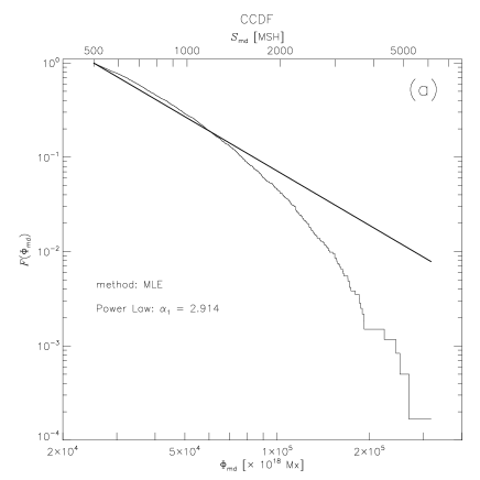
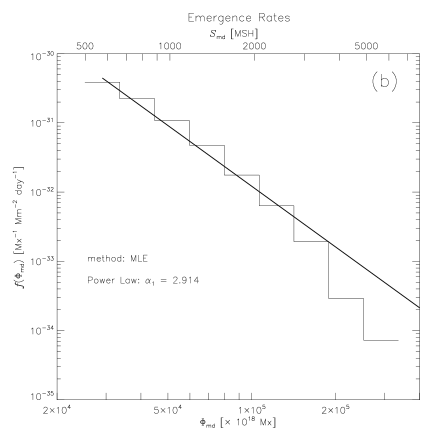
Figure 4: (a) An MLE power-law fit (straight line) to the complimentary cumulative distribution function of magnetic flux $F(\Phi)$. (b) The power-law fit of panel (a) for $F(\Phi)$ is converted to the probability distribution function $f(\Phi)$ and is overplotted on the histogram of the data.

Table 2: Derived parameters and 1-$\sigma$ error ranges

Model	Method	Parameter values and errors		$\Delta$AIC${}^{a}$	$\sqrt{N_{\rm s}}$ KS${}^{b}$	KS	KSr
						prob.${}^{c}$	P-value${}^{d}$
Power law
	MLE	$\alpha_{1}=2.914\pm 0.035$		184.6	4.14	$<10^{-6}$	0.019
Tapered power law
	MLE	$\alpha_{2}=1.808\pm 0.091$	$\beta_{2}=0.669\pm 0.056$	2.79	1.059	0.210	0.290
	KSr=min	$\alpha_{2}=1.886\pm 0.153$	$\beta_{2}=0.614\pm 0.083$	3.77	1.211	0.105	0.444
Gamma
	MLE	$\alpha_{3}=1.358\pm 0.138$	$\beta_{3}=0.591\pm 0.057$	1.51	0.989	0.279	0.458
	KSr=min	$\alpha_{3}=1.450\pm 0.224$	$\beta_{3}=0.547\pm 0.083$	2.11	1.08	0.195	0.665
Lognormal
	MLE	$\mu=-0.300\pm 0.099$	$\sigma=0.777\pm 0.035$	1.55	0.630	0.817	0.414
	KSr=min	$\mu=-0.157\pm 0.188$	$\sigma=0.728\pm 0.061$	4.27	1.075	0.196	0.490
Weibull
	MLE	$k=0.625\pm 0.044$	$\beta_{5}=2.278\pm 0.217$	0.00	0.827	0.497	0.911
	KSr=min	$k=0.629\pm 0.068$	$\beta_{5}=2.270\pm 0.396$	0.06	0.868	0.434	0.850

${}^{a}$: Relative AIC values with respect to the minimum value of all the AIC values.
${}^{b}$: Kolmogorov-Smirnov statistic KS derived from the observed data and the assumed model, multiplied by $\sqrt{N_{\rm s}}$.
${}^{c}$: Theoretical probability that the KS metric shows values larger than the observed KS metric.
${}^{d}$: Probability based on the simulation runs that the simulated KSr values are larger than the observed KSr value.

3.2 Models and Fitting Procedures

In this paper we will try to fit the observed data set $\Phi_{i}$ by

• a power-law distribution (parameter: $\alpha_{1}$),

• a tapered power-law distribution (parameters: $\alpha_{2},\beta_{2}$),

• a truncated gamma distribution (parameters: $\alpha_{3},\beta_{3}$),

• a truncated lognormal distribution (parameters: $\mu,\sigma$), and

• a truncated Weibull distribution (parameters: $k,\beta_{5}$).

A tapered power-law distribution (also called the Pareto distribution of the third kind (jkb94) in contrast to the original Pareto distribution which is a pure power law) has a CCDF that is a product of a power law and an exponential function. A gamma distribution has a PDF that is a product of a power law and an exponential function, and its CCDF is represented in terms of the gamma function. These have been used to describe the distribution functions of earthquake magnitudes (e.g. kag02; ser17), in comparison with the power-law distribution which is named the Gutenberg-Richter relation in seismology (e.g. uts99).

The power-law distribution is a one-parameter model while the other four are two-parameter models. Models (1), (2), and (3) have a power-law component with the exponent $\alpha_{1}$, $\alpha_{2}$, and $\alpha_{3}$, respectively. Models (2), (3), and (5) have an exponential component whose decay coefficients are represented by $\beta_{2}$, $\beta_{3}$, and $\beta_{5}$. The best-fit parameter values can be given systematically by the maximum-likelihood estimator (MLE), by maximizing the log-likelihood (LLH),

$${\rm LLH}=\sum\ln(P(\Phi_{i})).$$ (4)

The definitions of these five distributions and their MLE solutions are given in Appendix A.

Whether one model is more superior to the others can be assessed by comparing the AIC values (aka74),

$${\rm AIC}=-2\times\mbox{max(LLH)}+2K,$$ (5)

where $K$ is the number of parameters ($K=1$ or 2 in our analysis). (In another often-used criteria, Bayesian information criteria or BIC, $K\ln n$ ($n$ is the sample size) is used instead of $2K$; bur02.) By increasing the number of parameters, the fitting becomes better and LLH increases. However, the introduction of more parameters is not justified if AIC does not decrease. If the AIC value of one model is smaller than the AIC of the other by 9–11 or more, the former model is regarded better than the latter (bur11).

AIC is a relative measure, and it is possible that the model preferred by AIC still gives a poor fit. Whether the fitting by one model is not satisfactory and should be rejected can be estimated by evaluating a statistical measure that quantifies the difference between the observed and modeled CCDFs and by comparing that measure with a theoretical threshold (ste70; ste16). Here we use the Kolmogorov-Smirnov statistic KS defined by Equation (LABEL:eq:KS). For a large-enough $N_{\rm s}$, the probability for the observed $\sqrt{N_{\rm s}}$ KS value or larger to be obtained is theoretically given as a function (Kolmogorov-Smirnov function) which has relatively weak dependence on $N_{\rm s}$. Alternatively we can utilize simulation runs to estimate the probability (see below).

Once the parameter values are obtained, we can estimate their error ranges using the parametric bootstrap method (efr93; bur02) as follows.

• Generate $N_{\rm s}$ sets of uniform random variables $y_{i}$, $i=1,2,\ldots,N_{\rm s}\ (0\leq y_{i}\leq 1)$.

• Find $\Phi_{i}$ such that $F(\Phi_{i})=y_{i}$.

• For the data set $\Phi_{i}$ ($i=1,2,\ldots,N_{\rm s}$), obtain the MLE solutions for the parameters and the KS statistic.

• Repeat (1)–(3) $m$ times; then the distributions of the parameter values and the KS statistic are obtained.

• Evaluate the 1-$\sigma$ width of these distributions and adopt them as the error ranges of the parameters.

• For the KS statistic, if the number of cases where the KS values exceed the observed value KS${}_{\rm obs}$ is $m^{\prime}$, then $m^{\prime}/m$ gives the probability (P-value) that such a value of KS${}_{\rm obs}$ is obtained under the assumed model.

The 1-$\sigma$ values defined in step (5) scale basically as $1/\sqrt{N_{\rm s}}$ and do not depend on $m$ if it is taken sufficiently large (we used $m=10^{5}$).

The procedure described above has some points to consider. First, the MLE solution is not intended to geometrically fit a model CCDF to the observed CCDF. Particularly, it does not care much about the fitting at the tail, because the MLE solution is mostly determined by data points of highest density, i.e. near to the lower end of the distribution. A more geometrically-favorable solution may be obtained by, say, minimizing directly the KS statistic. Second, the KS statistic is not sensitive to misfitting at the lower and upper ends of the distribution, because by definition both the observed and model CCDF match (taking the values of 0 or 1) at the ends. It is known that the contributions to KS roughly scales as $1/\sqrt{F(1-F)}$ (and52), and cla09 suggested to use a modified form of the KS statistic by dividing its components by $1/\sqrt{F(1-F)}$ to enhance the sensitivity of the test at both ends. Here we introduce a KSr (revised KS) statistic defined by Equation (LABEL:eq:KSr), by dividing only by $1/\sqrt{F}$ to enhance the sensitivity at the tail.

In summary, we will apply two methods.

• Method 1: Seek the MLE solution, check the AIC values, and test the KS statistic by the Kolmogorov-Smirnov function. Then by simulation runs, estimate the error ranges of the obtained parameters, and the P-value of the observed KSr statistic.

• Method 2: Minimize KSr to obtain the solution, check the AIC values, and test the KS statistic by the Kolmogorov-Smirnov function. Then by simulation runs, estimate the error ranges of the obtained parameters, and the P-value of the observed KSr statistic.

Method 2 was not applied to the power-law model because the deviations of the model at the tail are large and the introduction of KSr may not make sense.

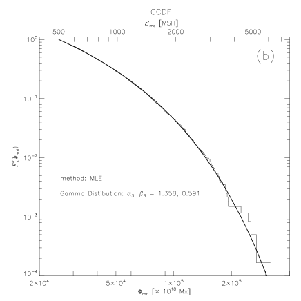
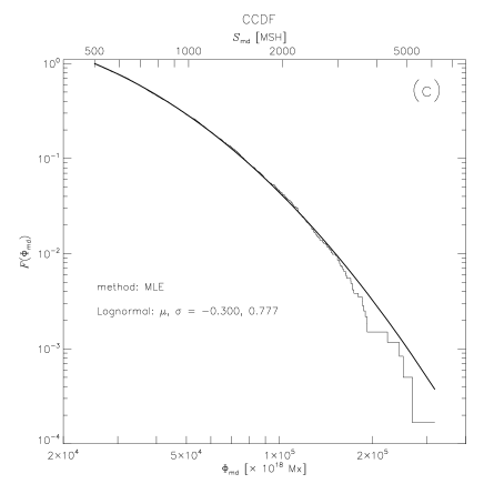
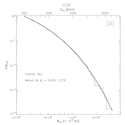
Figure 5: MLE fits to the complimentary cumulative distribution functions $F(\Phi)$ using models of (a) tapered power law, (b) gamma, (c) lognormal, and (d) Weibull distributions.

4 Fitting Results

4.1 Power Law

Figure 4 shows the results of power-law fitting. The MLE solution for the exponent is $\alpha_{1}=2.91$, and the KS statistic is large, $\sqrt{N_{\rm s}}$ KS = 4.1. Therefore, the probability of obtaining such a value or larger is infinitesimally small, and the model is safely rejected.

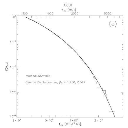
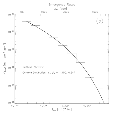
Figure 6: (a) A fit to the complimentary cumulative distribution function (CCDF) $F(\Phi_{\rm md})$ using the gamma distribution model and by minimizing the KSr metric. (b) The gamma-distribution fit of panel (a) for $F(\Phi_{\rm md})$ is converted to the probability distribution function $f(\Phi_{\rm md})$ and overplotted on the histogram of the data.

4.2 Two-Parameter Models

Figures 5 (a)–(d) show the results of fitting by adopting MLE solutions (Method 1). Method 2 also gives similar plots. In Figure 6, both the CCDF and emergence rates $f(\Phi_{\rm md})$ together with the fitted functions are given by applying Method 2 to the gamma distribution model, which is our most favorable model.

Table 2 summarizes, for MLE and KSr=min (except for power law) methods respectively, the obtained parameter values (with error ranges), relative AIC values, KS statistics and its theoretical probability, and P-values based on the KSr statistic. Here $\Delta$AIC ($\Delta$BIC = $\Delta$AIC among the two-parameter models) means the values of AIC with respect to its smallest value in the models (which happened to take place for the MLE model applied to the Weibull distribution). Strictly speaking, AIC is defined when LLH is maximized [the MLE solution, Equation (5)], but we also applied the same formula by replacing max(LLH) with LLH from a particular solution not maximizing LLH. Therefore, for each model, $\Delta$AIC is smaller for the MLE solution than for the solution with KSr=min. Likewise, the P-value based on KSr is larger (better fitting) for the solution with KSr=min compared to the MLE solution.

The following properties can be found on this table.

1. The AIC values of the two-parameter models are much smaller than the case of the power law, so that all these four models are better than the power law. The four models show $\Delta$AIC values less than 5 and cannot be discriminated.

2. From the KS probabilities, the MLE solutions show better performance but the KSr=min solutions are also acceptable.

3. From the P-values of the KSr metric, the solutions minimizing KSr show better performance but the MLE solutions are also acceptable.

4. The power-law indices of the tapered power law and the gamma distributions are $\alpha_{2}=$ 1.8–1.9 and $\alpha_{3}=$ 1.35–1.45. The reason why $\alpha_{2}>\alpha_{3}$ is given in Appendix LABEL:appendix:tapered-power-law; the tapered power-law distribution actually contains a mixture of two exponents $\alpha_{2}$ and $\alpha_{2}-1$, and its overall behavior is somewhere between them. If we extend the PDF toward smaller $\Phi_{\rm md}$ values, the tapered power-law distribution asymptotically approaches the power law with exponent $\alpha_{2}$. In any case it is important to point out that both distributions show the power-law-like behavior with exponent less than 2, namely the overall contributions to the magnetic flux supply come mostly from large $\Phi_{\rm md}$ regions.

5. As we discuss later (Figure 7), the behavior of lognormal and Weibull distributions extended to smaller values of $\Phi_{\rm md}$ is different from the tapered power-law and gamma distributions (the latter two behave essentially like a power law with exponent $\simeq$ 1.35–1.9). The Weibull distributions approach toward a very flat power-law distribution $\propto\Phi_{\rm md}^{-0.4}$, and the lognormal distributions decrease toward small $\Phi_{\rm md}$. Therefore, our preferred models are the tapered power-law and gamma distributions.

6. The tapered power-law and gamma distributions show a steep fall-off for large $\Phi_{\rm md}$ values, steeper than power laws, indicating that the probability of having extremely large active regions is vanishingly small and there is a practical upper limit in the size and magnetic flux of emerging active regions.

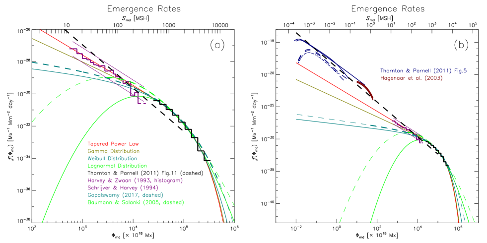
Figure 7: (a) Comparison of magnetic flux emergence rates $f(\Phi_{\rm md})$. The histogram drawn with a thick black line is our data. Four kinds of fits by minimizing the KSr metric are shown, respectively, for tapered power-law (red), gamma (olive), Weibull (teal green), and lognormal (lime green) distributions. The black dashed line of power-law exponent 2.69 is from tho11. The histogram shown in purple is from khz93, and the two parallel lines in purple are the power laws of exponent=2 (sch94) representing their amplitude ranges in solar activity minima/maxima. The dashed curve in lime green is the lognormal fit from bau05. The dashed curve in teal green is the Weibull function fit from gop18. (b) Same as panel (a) but the plotting range is extended to smaller flux values. Newly added graphs are the SOHO/MDI data from hst03 and the Hinode/SOT data from tho11.

5 Comparison with Published Results

In this section, we will compare our results on the two-parameter models with the published observational data and fitting results. In Figure 7a which shows the flux emergence rates $f(\Phi_{\rm md})$, the histogram in a thick black line is our data (500 MSH $\leq S_{\rm md}\leq$ 6132 MSH, $2.53\times 10^{22}\ {\rm Mx}\leq\Phi_{\rm md}\leq 3.18\times 10^{23}\ {\rm Mx}$). Four solid curves show our fits by minimizing the KSr metric; tapered power-law (red), gamma (olive), Weibull (teal green), and lognormal (lime green) distributions. They are extended down to $\Phi_{\rm md}=10^{20}$ Mx ($S_{\rm md}\simeq 2$ MSH) and up to $\Phi_{\rm md}=10^{24}$ Mx ($S_{\rm md}\simeq 19000$ MSH). Toward the smaller ends of $\Phi_{\rm md}$, the tapered power-law, gamma, and Weibull distributions approach power laws with exponents 1.89, 1.45, and 0.37, respectively

The histogram in a thick purple line is taken from khz93, who derived the emergence rates of bipolar active regions using the data obtained at NSO Kitt Peak (liv76). sch94 reported that this distribution is fitted by a power law with exponent 2, and the amplitudes vary by roughly a factor of 10 between activity minimum and maximum, as shown by two parallel lines in purple.

The thick dashed curve in lime green reproduces the lognormal fit to the RGO data ($S_{\rm md}\geq$ 60 MSH) by bau05, extended down to $S_{\rm md}\simeq 2$ MSH (thin dashed curve). Below the peak at $S_{\rm md}\simeq 62.2$, the curve goes down to $f\rightarrow 0$. Our lognormal fit peaks at $S_{\rm md}\simeq$ 250 MSH and then decreases to $f\rightarrow 0$. At least for our lognormal fitting, this decrease is not due to small fluxtubes losing their darkness, because even the smallest regions (500 MSH) in our sample are fairly large regions. Rather, this is a result of the shape of the observed distribution that bends down toward large $\Phi_{\rm md}$, and the derived $\mu$ value may not represent any physical significance. bog88 gave the values 0.34–0.62 MSH for the peak of the instantaneous distribution function of sunspot umbral areas modeled by lognormal distribution.

The thick dashed curve in teal green reproduces the Weibull fit to the RGO and USAF/NOAA data by gop18, which covered all the data $S_{\rm md}\geq 1$ MSH. The curve is very close to our Weibull fit.

In Figure 7b, we extended the plot range to $10^{15}$ Mx $\leq\Phi_{\rm md}\leq 10^{25}$ Mx ($2.3\times 10^{-5}$ MSH $\lesssim S_{\rm md}\lesssim 1.9\times 10^{5}$ MSH), and added two more data sets. The thick solid curve in brown is from hst03, who investigated the emergence rates of small-scale bipolar magnetic patches (ephemeral regions) using the data from SOHO/MDI. The thick curves in navy blue (solid, dashed, dotted) are from tho11, who analyzed the emergence rates of small-scale magnetic patches using the data from Hinode/SOT. The thin dashed line in teal green is the downward extension of gop18’s Weibull distribution.

The thick dashed lines in black in Figures 7a and 7b show the power law of exponent 2.69 suggested by tho11 to cover all the way from small-scale flux concentrations to large active regions. Our picture is different from theirs; the flux emergence rates of active regions are characterized by a power-law-like behavior of exponents between 1.45 (olive) and 1.89 (red) in Figure 7. Our results are roughly consistent with the observations by khz93, who also showed that the distribution amplitudes varied by a factor of 10 between activity minima and maxima. Ephemeral regions and much smaller flux concentrations may have a power-law distribution with exponent 2.69, but they show little changes (or even anti-phase changes; hst03) with the solar cycle, and they may give way to the active region component somewhere at around $\Phi_{\rm md}\simeq 10^{20}$ Mx. The exponent larger than 2 in small-scale flux concentrations means dominant contributions of flux emergence in the smallest end of the distribution function. Those small-scale flux emergence may be sustained by a local dynamo (cat99; bue13). The total (unsigned) magnetic flux on the Sun in scales exceeding a few arcseconds ($\gtrsim 1000$ km) varies in phase with the solar cycle (arg02), and the flux at activity maximum is about four times the flux at minimum. Therefore, flux emergence in small scales would not accumulate to systematically overwhelm the magnetic flux from active regions.

Table 3: Sunspot area, magnetic flux, and interval of appearance

$S$ [MSH]	$\Phi$ [Mx]	Interval [year]
500	$2.5\times 10^{22}$	$5.242\pm 0.001\times 10^{-2}$
1000	$5.1\times 10^{22}$	$1.82\pm 0.04\times 10^{-1}$
2000	$1.0\times 10^{23}$	$1.20\pm 0.04\times 10^{0\phantom{-}}$
3000	$1.5\times 10^{23}$	$6.0^{+0.9}_{-0.8}\times 10^{0\phantom{-}}$
6132	$3.2\times 10^{23}$	$5.2^{+3.7}_{-2.2}\times 10^{2\phantom{-}}$
10000	$5.2\times 10^{23}$	$8.2^{+17}_{-5.5}\times 10^{4\phantom{-}}$

$S$ [MSH]	$\Phi$ [Mx]	Interval [year]
$6.2^{+0.5}_{-0.4}\times 10^{3}$	$(3.2^{+0.2}_{-0.2})\times 10^{23}$	$1.0\times 10^{3}$
$7.9^{+0.7}_{-0.5}\times 10^{3}$	$(4.1^{+0.4}_{-0.3})\times 10^{23}$	$1.0\times 10^{4}$
$9.7^{+1.0}_{-0.7}\times 10^{3}$	$(5.0^{+0.5}_{-0.4})\times 10^{23}$	$1.0\times 10^{5}$
$1.15^{+0.12}_{-0.09}\times 10^{4}$	$(6.0^{+0.6}_{-0.5})\times 10^{23}$	$1.0\times 10^{6}$
$1.51^{+0.18}_{-0.14}\times 10^{4}$	$(7.9^{+1.0}_{-0.7})\times 10^{23}$	$1.0\times 10^{8}$
$1.83^{+0.23}_{-0.17}\times 10^{4}$	$(9.6^{+1.2}_{-0.9})\times 10^{23}$	$4.6\times 10^{9}$

The ranges of values are based on the 1-$\sigma$ error ranges given in Table 2, namely $\alpha_{3}=1.450\pm 0.224$, $\beta_{3}=0.547\pm 0.083$.

5.1 Emergence Frequency of Large Sunspots

Based on the fitting results, we are able to predict the expected frequencies of large sunspots. Table 3 shows, by using the model of gamma distribution with parameter values determined from KSr=min ($\alpha_{3}=$ 1.450 $\pm$ 0.224, $\beta_{3}=$ 0.547 $\pm$ 0.083), the expected appearance intervals as a function of sunspot area (left half of the table), and the expected sunspot areas for the specified values of appearance intervals (right half of the table). The ranges of values given are based on the 1-$\sigma$ error ranges given in Table 2. It turned out that the errors in $\alpha_{3}$ and $\beta_{3}$ are roughly inversely correlated, so that the ranges of values shown in Table 3 correspond to $(\alpha_{3},\beta_{3})=$ (1.450 + 0.224, 0.547 $-$ 0.083) and (1.450 $-$ 0.224, 0.547 + 0.083).

The time interval for regions with flux larger than $\Phi$ to appear is given by $[F(\Phi)N_{\rm s}/T]^{-1}$ ($N_{\rm s}$ = 2995, $T=$ 146.7 years). The sunspots larger than 500 MSH are expected to appear at a rate of every 19 days. The regions as large as or exceeding the largest region in our database (6132 MSH) are expected to appear every 520 years. Beyond roughly 10000 MSH, the interval becomes longer than $8\times 10^{4}$ years, and even after the lifetime of the Solar System ($4.6\times 10^{9}$ years), one can only expect a region as large as 1.8 $\times 10^{4}$ MSH. These are due to the exponential decline of the probability distribution function. By taking into account the 1-$\sigma$ errors, the expected interval for 10000 MSH regions is reduced to 2.7 $\times 10^{4}$ years, and 2.1 $\times 10^{4}$ MSH is the possible maximum size after $4.6\times 10^{9}$ years.

Figure 8: A model for sunspot area evolution proposed by kop56. (a) The area $S(t)$ as a function of time $t$ in day is given for a set of parameters $(a,b)=(0.3,20.0)$, by changing $K$. The curves correspond, from the lowest to the highest, to the maximum-development areas $S_{\rm md}$ of 500, 1000, 2000, 4000, and 6132 MSH. (b) The lifetime $t_{\rm life}$ as a function of maximum-development area $S_{\rm md}$. The thick solid line is our adopted model with $(a,b)=(0.3,20.0)$, while the dashed line represents the original relation of kop56 with $(a,b)=(0.3,4.0)$. The dotted lines are the formulae given by gne38 and nag19, respectively. The diamond signs and asterisks denote the lifetimes of regions taken from published data (kop84; rgo55).

6 Forward Modeling

In the analysis so far, we have assumed that the maximum sunspot areas observed on the visible hemisphere are the true maximum areas, which might take place on the back side of the Sun, though. The errors caused by this assumption cannot be corrected, but we may be able to estimate the effects by a forward modeling, namely, by assuming a typical time evolution of sunspot areas we can simulate such effects. As a biproduct, we can convert our maximum-development distribution functions to instantaneous distribution functions.

Figure 9: Effects of time evolution of sunspot areas were estimated by using a model by kop56. The dashed curve is the model generated from a gamma distribution with $\alpha_{3}=$ 1.450 and $\beta_{3}=$ 0.547 which reproduces the data well. The solid curve shows the distribution expected from the model by taking into account the visibility probability of regions.

6.1 Model

Many models have been proposed to represent the time evolution of sunspot areas (e.g. kop56; ant86; how92; hat08). Here we use the model proposed by kop56 because of its analytical simplicity and versatility. The time evolution of sunspot area $S(t)$ is described by a differential equation

$$\frac{{\rm d}S}{{\rm d}t}=-aS+K-bt\qquad(t\geq 0),$$ (6)

where $a$, $b$, and $K$ are parameters; $(a,b)$ control the shape of the time profile, and $K$ controls the maximum size of the region. The solution to this equation is given as

$$S=\frac{1}{a}\left[\left(K+\frac{b}{a}\right)\left(1-{\rm e}^{-at}\right)-bt\right],$$ (7)

and $S(t)$ takes the maximum value

$$S_{\rm md}=\frac{K}{a}-\frac{b}{a^{2}}\ln\frac{aK+b}{b}$$ (8)

at time

$$t_{\rm md}=\frac{1}{a}\ln\frac{aK+b}{b}.$$ (9)

$S(t)$ starts from $S(0)=0$ and comes back to $S(t_{\rm life})=0$ where

$$\frac{1-\exp(-at_{\rm life})}{at_{\rm life}}=\frac{b}{aK+b}.$$ (10)

The solution for $t_{\rm life}$, if $at_{\rm life}\gg 1$, is

$$t_{\rm life}\simeq\frac{K}{b}+\frac{1}{a},$$ (11)

and if $at_{\rm life}\ll 1$, it is

$$t_{\rm life}\simeq\frac{2K}{aK+b}.$$ (12)

kop56 used the empirical relations $t_{\rm life}{\rm[days]}\simeq 0.1S_{\rm md}{\rm[MSH]}$ (gne38) and $t_{\rm life}/t_{\rm md}\simeq 0.094S_{\rm md}{\rm[MSH]}+9.3$ (kop53) and adopted $(a,b)=(0.3,4.0)$ which roughly reproduces these empirical relations for $S_{\rm md}\lesssim 400$ MSH. However, this setting makes the lifetimes of 500 MSH (minimum in our database) and 6132 MSH (maximum) regions as 50 days (1.8 solar rotations) and 480 days (1.3 years, 17.6 solar rotations) respectively, which look too long. nag19 suggested $t_{\rm life}{\rm[days]}\simeq 0.077S_{\rm md}{\rm[MSH]}$, a slightly shorter lifetime for the specified $S_{\rm md}$ compared to gne38, but this also gives large values of lifetimes. According to kop84 the longest lifetime of regions in the RGO observations was 8 solar rotations (RGO recurrent series No. 2094, 1970 June 11 – December 23, 195 days, maximum area = 1774 MSH). The region of largest area (RGO region 14886, 6132 MSH) had a lifetime of 95 days (1947 February 5 – May 11, observed for 4 rotations).

As will be discussed in Section LABEL:sec:instantaneous, the gamma function model for $F(\Phi_{\rm md})$ described in Section 5.1 gives the instantaneous distributions of sunspot area or magnetic flux which are consistent with the observed distributions only if the region lifetimes are much shorter; a reasonable value we found is $(a,b)=(0.3,20.0)$. The value of $a$ is fixed to 0.3, because the rise time of region growth ($\simeq 1/a$) does not strongly depend on the region size. The lifetimes of the 500 and 6132 MSH regions in this model are 16 and 107 days, respectively. Figure 8a shows the time profiles $S(t)$ derived for $(a,b)=(0.3,20.0)$ and for several values of $S_{\rm md}$. Figure 8b compares the models with $(a,b)=(0.3,4.0)$ and $(0.3,20.0)$, and other published results of sunspot lifetimes. The diamond signs denote the data points of three longest-lived regions listed in kop84. The asterisks denote the lifetimes of maximum sunspot areas $>3000$ MSH taken from rgo55. The regions whose emergence or decay (either of them) were not observed on the visible disk have uncertainties in their lifetimes between 1 and 13 days. Hence we roughly assigned a 7-day error bar. The regions whose emergence and decay (both of them) were not observed on the visible disk were assigned with a 14-day error bar. The model with $(a,b)=(0.3,20.0)$ goes through the middle of the data points representing large ($>3000$ MSH) regions.

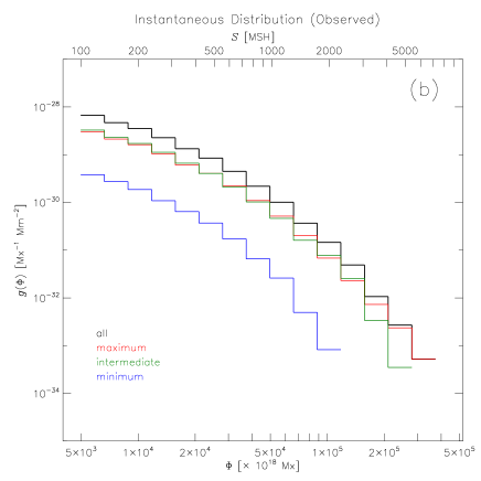
Figure 10: (a) The histogram of the probability distribution function $g(\Phi)$ of instantaneous distribution of magnetic flux, derived from a gamma distribution with $\alpha_{3}=$ 1.450 and $\beta_{3}=$ 0.547 combined with the sunspot area evolution models of Figure 8. The solid and dashed histograms correspond to $(a,b)=(0.3,20.0)$ and $(a,b)=(0.3,4.0)$, respectively. (b) The corresponding distributions derived from observations of RGO and NOAA. The histogram in black was derived by using all the data with areas larger than 100 MSH, while red, green, and blue ones are based on data from maximum, intermediate, and minimum phases of activity defined in Table 4.

6.2 Effects of Time Evolution

The effects of time evolution of sunspots were simulated as follows. By adopting a model of gamma distribution with $\alpha_{3}=$ 1.450 and $\beta_{3}=$ 0.547, we have generated $N_{\rm s}$ samples ($N_{\rm s}=$ 2995) of $\Phi_{\rm md}$ by

$$F(\Phi_{i})=\frac{i-0.5}{N_{\rm s}}\quad(i=1,2,\ldots,N_{\rm s}).$$ (13)

Then each model was placed at 27 equal-distant longitudes (27 is a rough number of solar rotation period in days), magnetic flux was converted to sunspot area by Equation (1), and was evolved according to Equation (7). The observed maximum values of $S(t)$ in the longitude ranges of $\pm 80^{\circ}$ were recorded, converted to magnetic flux, and the CCDF was generated.

The solid curve in Figure 9 shows the result, compared with the true distribution designated by the dashed curve. After fitting the model, we found $\alpha_{3}=$ 1.319 and $\beta_{3}=$ 0.590. The flattening of the distribution from $\alpha_{3}=$ 1.450 to $\alpha_{3}=$ 1.319 (by about 0.13) is because we underestimated $S_{\rm md}$, and the data points on the original model (dashed) were shifted toward left on the graph. From this we may estimate that $\alpha_{3}=$ 1.450 derived from observations would actually be around $\alpha_{3}=$ 1.68, but still our conclusion will hold that the power-law exponent is less than 2.

Table 4: Summary of observed quantities

Data	Time	Regions per	Daily region counts	Number of	Observed maximum values
source	span	full Sun${}^{a}$	per hemisphere	observations	Total	Total	Region	Region
		$N_{\rm s}$	$N_{\rm rd}$	$N_{\rm d}$	area	flux	lifetime	counts
	[year]	$(S_{\rm md}\geq$	($S\geq$	($S_{\rm hs}\geq$	[MSH]	[Mx]	[d]
		500 MSH)	500 MSH)	10 MSH)
All	146.71	2995	$1.97\times 10^{4}$	$4.42\times 10^{4}$	8382${}^{b}$	$4.36\times 10^{23}$	195${}^{c}$	26${}^{d}$
Maximum	35.26	1466	$0.99\times 10^{4}$	$1.28\times 10^{4}$	8382${}^{\phantom{b}}$	$4.36\times 10^{23}$
Minimum	37.65	114	$0.06\times 10^{4}$	$0.71\times 10^{4}$	2268${}^{\phantom{b}}$	$1.16\times 10^{23}$
Intermediate	73.80	1415	$0.92\times 10^{4}$	$2.43\times 10^{4}$	8080${}^{\phantom{b}}$	$3.54\times 10^{23}$

${}^{a}$ Recurrent regions were manually picked up and counted only once when they showed the largest area.
${}^{b}$ 1947 April 8
${}^{c}$ RGO recurrent series No. 2094, 1970 June 11 – December 23 (kop84).
${}^{d}$ 1937 July 12