Learning General Audio Representations
With Large-Scale Training of Patchout Audio Transformers

Abstract

The success of supervised deep learning methods is largely due to their ability to learn relevant features from raw data. Deep Neural Networks (DNNs) trained on large-scale datasets are capable of capturing a diverse set of features, and learning a representation that can generalize onto unseen tasks and datasets that are from the same domain. Hence, these models can be used as powerful feature extractors, in combination with shallower models as classifiers, for smaller tasks and datasets where the amount of training data is insufficient for learning an end-to-end model from scratch. During the past years, Convolutional Neural Networks (CNNs) have largely been the method of choice for audio processing. However, recently attention-based transformer models have demonstrated great potential in supervised settings, outperforming CNNs. In this work, we investigate the use of audio transformers trained on large-scale datasets to learn general-purpose representations. We study how the different setups in these audio transformers affect the quality of their embeddings. We experiment with the models’ time resolution, extracted embedding level, and receptive fields in order to see how they affect performance on a variety of tasks and datasets, following the HEAR 2021 NeurIPS challenge evaluation setup. Our results show that representations extracted by audio transformers outperform CNN representations. Furthermore, we will show that transformers trained on Audioset can be extremely effective representation extractors for a wide range of downstream tasks.

Keywords: Representation Learning, Audio Processing, Transformers, CNNs

1 Introduction

The high cost and scarcity of high-quality labeled data is a significant impediment to applying deep learning methods to audio classification and tagging tasks. One popular alternative is to use models pre-trained on large-scale and broad datasets (Gemmeke et al., 2017; Abu-El-Haija et al., 2016) to obtain high-quality and relevant representations from raw waveforms, which can improve performance on downstream tasks. Audioset (Gemmeke et al., 2017) is a dataset of annotated clips from Youtube videos. The dataset contains approximately 2 million audio clips of 10 seconds each. Each clip is assigned tags representing the acoustic events occurring in the clip. There are 527 possible classes that are taken from the Audioset ontology (Gemmeke et al., 2017). The ontology covers a wide variety of events that include human and animal sounds, music, sounds of nature and things, and environments and backgrounds. Given the size and diversity of the dataset, it has been widely used to pre-train acoustic models with the goal of either fine-tuning these models on smaller datasets or extracting general features and representations out of raw audio waveforms (Kong et al., 2020; Plakal and Ellis, 2022; Cramer et al., 2019; Koutini et al., 2022).

The most common approaches for extracting audio presentation from raw waveforms has been to use pre-trained architectures based on Convolutional Neural Networks (CNNs) (Hershey et al., 2017; Cramer et al., 2019; Schneider et al., 2019). This is primarily due to the success of CNNs in various audio processing tasks and applications (Kong et al., 2020; Hershey et al., 2017; Koutini et al., 2021). VGGish (Hershey et al., 2017) is an example of a large-scale pre-trained CNN that is used to obtain features on which a task-specific classifier is trained (Humphrey et al., 2018). Arandjelovic and Zisserman (2017) propose a self-supervised multi-modal approach (L³-Net) to learn audio representations without the need for labels. Cramer et al. (2019) use AudioSet to train L³-Net, resulting in representations that outperform the VGGish model on a variety of tasks. Kong et al. (2020) introduced an improved CNN architecture that significantly improves on the VGGish model on Audioset. They also test transfer learning from models trained on Audioset to other tasks. They show that either fine-tuning or using the pre-trained CNN as a feature extractor can both help on some downstream tasks, such as acoustic scene classification and music genre classification.

Transformer models (Vaswani et al., 2017) have shown to be quite effective and have improved upon CNNs in many domains. Transformers enable the learning of relationships between distinct elements in sequences, independent of their placement or distances. Transformers have delivered state-of-the-art results in a variety of natural language processing applications (Devlin et al., 2019). The architecture was ported to computer vision (Dosovitskiy et al., 2021) by extracting patches from the input images and augmenting each patch using a learnable positional encoding. The resulting patches create a sequence that can be processed by a Transformer model.

Vision transformer models achieve state-of-the-art performance on different image classification tasks(Dosovitskiy et al., 2021; Touvron et al., 2021) as well as audio tagging and classification tasks (Gong et al., 2021; Koutini et al., 2022). However, they have a number of disadvantages, including high training complexity and cost, the need for a large amount of data, and the difficulty of adapting the learned positional encodings for variable-sized input. In order to overcome these problems, a large private dataset was used in the case of Vision Transformer (Vit) (Dosovitskiy et al., 2021). The authors of Data-efficient Image Transformers (DeiT) (Touvron et al., 2021) used a wide range of data augmentation methods and knowledge distillation from CNNs. The authors of Audio Spectrogram Transformer (AST) (Gong et al., 2021) leveraged the models’ pre-training on vision tasks to train on spectrograms. Patchout Audio Transformer (PaSST) (Koutini et al., 2022) addresses the problem of training complexity by significantly lowering the compute and memory requirements for spectrogram training with Patchout. Patchout is also a regularization method that improves the models’ generalization. PaSST separates time and frequency positional encodings, allowing for simple inference on shorter audio clips without the need to re-train or interpolate positional encodings.

In this paper, we investigate the extraction of general-purpose representations from pre-trained PaSST. We evaluate the extracted representations using HEAR-eval (Turian et al., 2022) on a wide range of audio tasks. We investigate various representation levels, spectrogram time resolutions, and input receptive fields. We compare the quality of our representation to that of widely used models. The study results will demonstrate that large-scale supervised training of transformers can yield powerful feature extractors that outperform CNNs trained on the same dataset and are competitive with task-specific models.

2 Patchout Fast Spectrogram Transformer (PaSST)

In this section, we will go over the model architecture as well as the training approach. The Patchout faSt Spectrogram Transformer (PaSST) (Koutini et al., 2022), which is based on the Vision Transformer architecture (Dosovitskiy et al., 2021), is used. Applying Patchout (Koutini et al., 2022) during model training significantly reduces model training time and acts as a regularizer to improve model generalization. Furthermore, disentangled time and frequency positional encodings in PaSST are critical for predicting on shorter audio clips and restricting the model’s receptive field, which is required to produce timestamp embeddings.

2.1 Vision Transformers

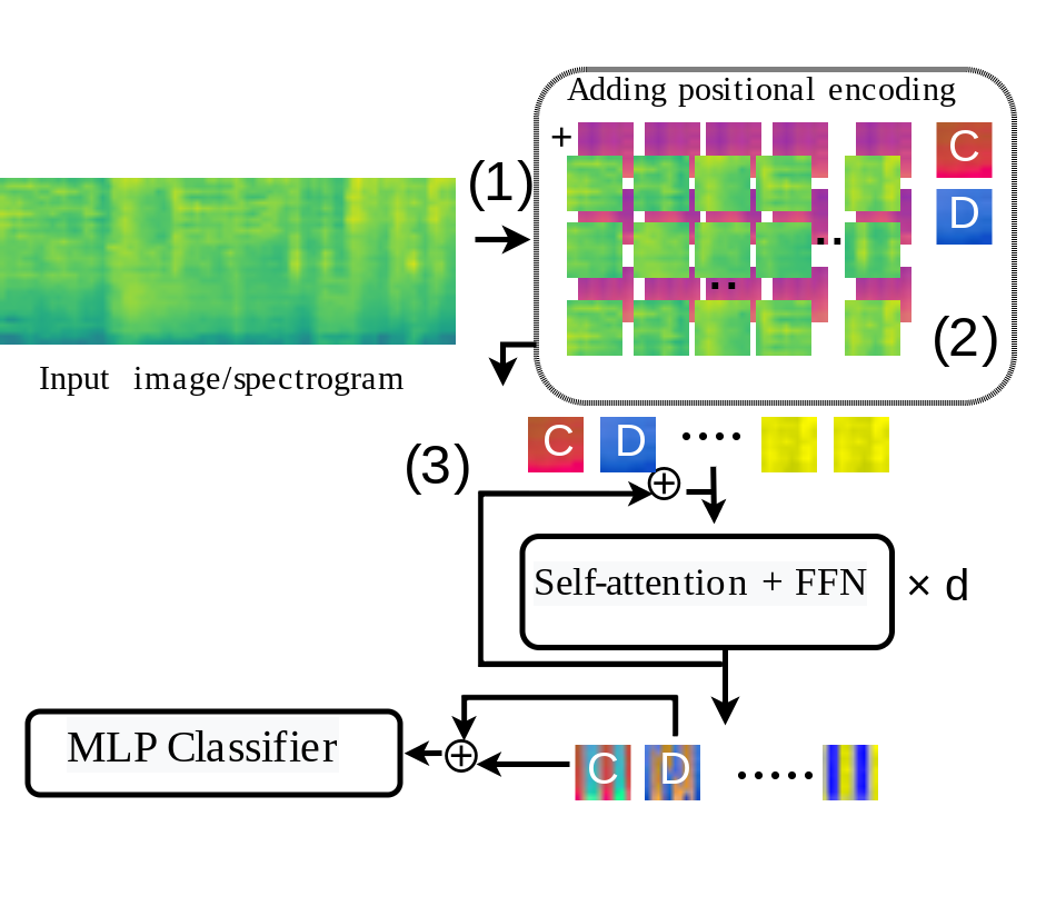
Figure 1: The Architecture of ViT (Dosovitskiy et al., 2021), DeiT (Touvron et al., 2021) and AST (Gong et al., 2021). C,D are the classification and distillation tokens.

The Vision Transformer (ViT) (Dosovitskiy et al., 2021) extracts small patches from an input image and projects them linearly onto a sequence of embeddings (Step 1 in Figure 1). Each element’s position in the sequence is then provided in the form of a bias, which is added to each embedding (Step 2 in Figure 1). Each of these positional encodings (biases) is a trainable parameter that aids in carrying information about the patch’s position in the original image (Dosovitskiy et al., 2021). The embedding sequence is supplemented with a special classification embedding (classification token C in Figure 1). Following the self-attention layers, the classification token is linked to a classifier. Another special embedding for distillation (distillation token D in Figure 1) is added in Data-efficient image Transformers (DeiT) (Touvron et al., 2021). DeiT has a similar architecture to ViT, but uses CNN distillation and data augmentation to reduce the amount of training data needed to train the transformer models. Audio Spectrogram Transformer (AST) (Gong et al., 2021) uses the same architecture applied to audio spectrograms. AST leverages pre-training on vision datasets to achieve good performance on Audioset (Gemmeke et al., 2017).

PaSST (Koutini et al., 2022) differs from previous models in two ways (Figure 2): first, it disentangles positional encodings into time and frequency positional encodings. Second, during training, a regularization strategy named Patchout is used. The following sections will go into these in detail. In summary, PaSST operates in the manner depicted in Figure 2: (1) Extract patches from the spectrogram (2) Augment these patches with time and frequency encondings (3) Use Patchout, and then (4) run the resulting sequence through the transformer.

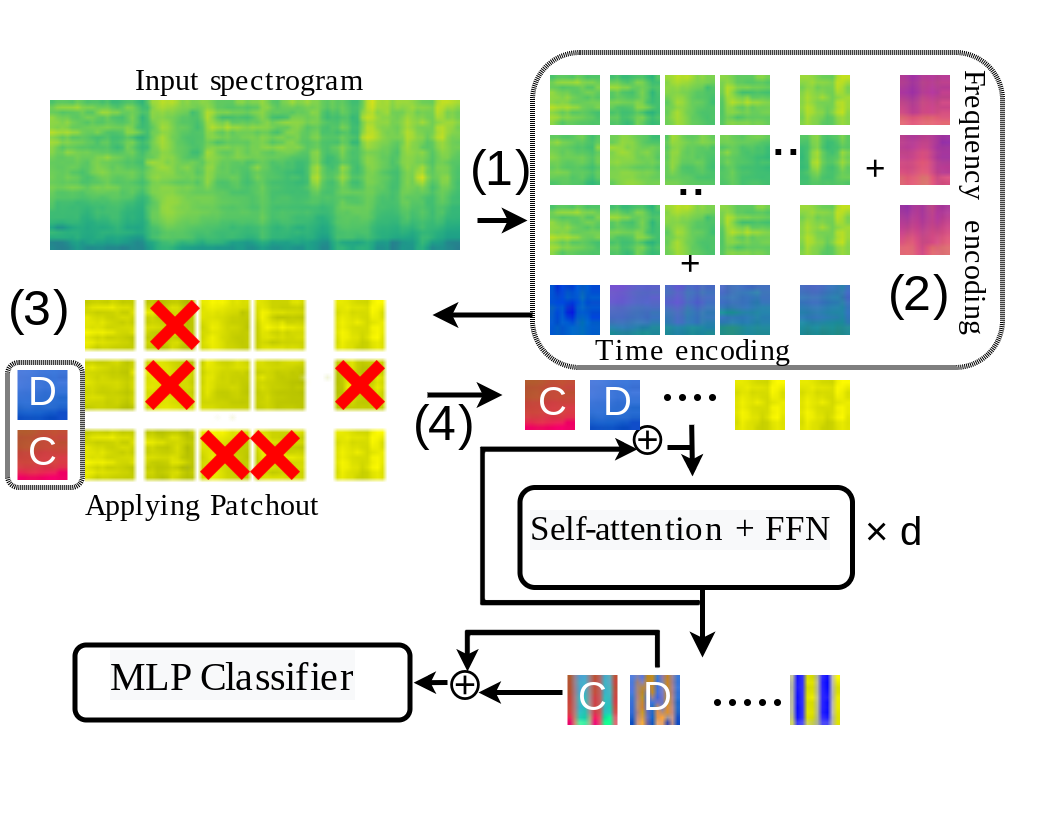
Figure 2: The Architecture of PaSST (Koutini et al., 2022). The distinction between Figures 1 and 2 is in disentangling the positional encodings into time and frequency positional encodings. In addition, patchout is used during training.

2.2 Patchout

Patchout (Koutini et al., 2022) works on the basic principle of dropping parts of the transformer’s input sequence during training, training the transformer to perform classification using an incomplete sequence. Reducing the sequence length both regularizes the model and significantly reduces the complexity of the training process. During inference, the entire input sequence is presented to the transformer, similar to DropOut (Srivastava et al., 2014). We distinguish the following types of Patchout:

Unstructured Patchout: is the most basic form, in which the patches are chosen at random regardless of their position.

Structured Patchout: We select some frequency bins / time frames at random and remove an entire column or row of extracted patches, similar in spirit to SpecAugment (Park et al., 2019). In the remainder of this work, we use only Structured Patchout since Koutini et al. (2022) showed that it performs better on Audioset.

Figure 3 shows that applying Patchout significantly reduces the training complexity while improving generalization. The figure shows that with structured Patchout, PaSST-S achieves higher performance on Audioset with 4 times the training speed of AST (Gong et al., 2021) and a fraction of the required memory. Furthermore, PaSST-N-S (with structured patchout and no patch overlap) outperforms CNNs with similar memory requirements and faster training.

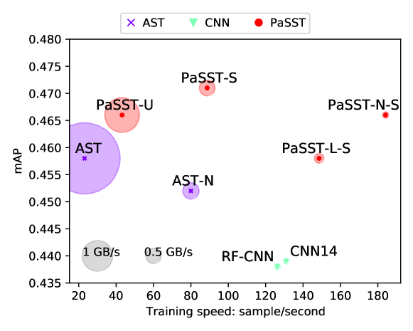
Figure 3: Prediction performance on Audioset (mean average precision) vs. training speed (samples per second). The radius of the circle indicates the required GPU memory (in gigabytes) per training sample. The figure shows PaSST variants (Koutini et al., 2022) with Structured Patchout (denoted by -S) and Unstructured Patchout (denoted by -U) compared with AST (Gong et al., 2021), CNN14 (Kong et al., 2020) and RF-CNNs (Koutini et al., 2019b). The PaSST variants marked with -L and -N are low-complexity and no-patch-overlap variants, respectively. PaSST-S achieves state-of-the-art Audioset performance in less than two days on a single consumer GPU. Source: (Koutini et al., 2022, Figure 1).

In this paper, we will use the PaSST-S variant, which has the best performance on Audioset. Section 4 discusses how we extract the embeddings of this model.

2.2.1 Computational complexity

Transformers primary building blocks are attention layers (Vaswani et al., 2017). Attention layers compute a distance between each pair of items in the input sequence, and these distances form the attention weights, resulting in a quadratic complexity with respect to the input sequence length, which in turn is a function of the length of the audio clips, the spectrogram resolution in time or frequency, and the patches overlap. As the sequence length $n$ grows, the computation complexity (and memory requirements) for the attention layers grows quadratically $\mathcal{O}(n^{2})$  (Koutini et al., 2022, Section 2.1). In short, reducing the length of the input sequences to self-attention layers would have a significant impact on the computational complexity of these models; Patchout addresses this issue.

2.2.2 Regularization Effect

Previous work has shown that, in the case of CNNs, restricting the receptive field on audio spectrograms during training improves their generalization on a variety of audio tagging and classification tasks (Koutini et al., 2021). Patchout has a similar effect on transformers by removing parts of the input spectrograms at random during training. While in CNNs the receptive field can be easily controlled via depth and kernel sizes (Koutini et al., 2021), transformers by design have a large receptive field and exploit distant dependencies in their input. That allows them to learn complex rules from their input, but can also lead to over-fitting, which is one of the reasons why transformers require a large amount of data and augmentations. Patchout ameliorates this problem by forcing the transformer to learn from incomplete and augmented spectrograms. Structured Patchout, specifically, is also similar to SpecAugment (Park et al., 2019), a data augmentation technique specific to spectrograms that helps in various audio tasks. Koutini et al. (2022) showed that Patchout leads to improvements in different datasets.

2.3 Disentangling Positional Encoding

The second distinction between PaSST (Koutini et al., 2022) and vision transformers (Dosovitskiy et al., 2021; Touvron et al., 2021; Gong et al., 2021) is that in PaSST, the positional encoding is disentangled into frequency and time encoding (see Figures 1 and  2). This simplifies predicting on audio clips of varying lengths, due to the fact that the learned frequency encoding does not need to be changed and is unaffected by the length of the audio clip. All that is needed is is to change the time encoding. Cropping the time encoding- to match the length of the audio clip- is a simple yet effective way for inference. This, however, does not address the issue of inference on audio clips that are longer than the ones on which the model was trained (10 seconds in Audioset), because the time encoding is only learned to cover 10 seconds of audio during training. As explained in Section 4, we address this by taking the mean of the embeddings extracted from overlapping 10-second windows. We leave learning time encodings for longer audio clips using improved training algorithms for future work.

3 General Evaluation of Audio Representations

This section explains the diverse audio tasks and the setup used to evaluate the representations extracted from the pre-trained PaSST models. We use the same setup and tasks used in the Holistic Evaluation of Audio Representations (HEAR) NeurIPS 2021 challenge.

3.1 Evaluation Tasks

The goal is to evaluate the models based on the quality of their generated representations across a wide range of tasks and scenarios. The tasks involve both short and long time spans and cover a wide range of audio domains, including speech, environmental sound, and music.

HEAR consists of nineteen diverse tasks. Turian et al. (2022) provide a detailed description of the tasks and the setup of each task for HEAR evaluation. We divided the tasks into three categories based on the audio domain and summarize the tasks and their datasets below:

• Speech: Contains all the tasks that consist of verbal articulations by humans.

  • Speech Commands 5hr: Spoken command recognition and classification, described in (Warden, 2018).

  • Speech Commands Full: Spoken command recognition and classification using 27 hours of data.

  • CREMA-D: The goal is to classify one of six different emotions (anger, disgust, fear, happiness, neutral, or sad) from a spoken sentence (Cao et al., 2014). The dataset contains $7,438$ 5-second audio clips.

  • LibriCount: The goal of this task is to count the number of speakers in an audio clip (Stöter et al., 2018). The dataset contains $5,720$ 5-second audio clips.

  • VoxLingua107 Top10: The task is to classify the language spoken in an audio clip into one of ten different languages (Valk and Alumäe, 2021). There are $972$ clips totaling about five hours of audio in the dataset.

• Music: Contains all tasks consisting of instrumental sounds:

  • NSynth Pitch 5hr: Instrumental sound classification from the NSynth Dataset (Engel et al., 2017) into one of 88 pitches.

  • NSynth Pitch 50hr: Similar to NSynth Pitch 5hr but with more training data.

  • Beijing Opera Percussion: The goal is to classify four main categories of percussion instruments (Tian et al., 2014). The dataset contains $236$ 5-second audio clips.

  • GTZAN Genre: The task is to classify a 30-second audio track into one of ten possible genres (Tzanetakis and Cook, 2002). The dataset contains $1,000$ tracks.

  • MAESTRO 5hr: The task is to perform music transcription using the MAESTRO dataset (Hawthorne et al., 2019).

  • Mridangam Stroke: The goal is to classify 10 different strokes using the Mridangam Stroke Dataset (Anantapadmanabhan et al., 2013). The dataset contains $6,977$ audio clips.

  • Mridangam Tonic: The goal is to classify the 6 different tonics of the Mridangam Stroke Dataset.

• General: Contains mostly environmental sounds and acoustic scenes, but also others that cannot be clearly put into either Speech or Music (like GTZAN Music Speech):

  • DCASE 2016 Task 2: Office sound event detection task, adapted from the DCASE 2016 Challenge (Lafay et al., 2017). The dataset consists of 72 audio clips, each lasting 2 minutes.

  • Beehive States: The goal is to identify the absence of the queen in a beehive (Nolasco et al., 2019). This dataset contains 930 clips that are approximately 10 minutes long.

  • ESC-50: The task is environmental sound classification  (Piczak, 2015). The dataset contains $2,000$ 5-second audio clips, each of which is classified into one of fifty categories.

  • FSD50K: The task is a general-purpose multi-label sound event detection task (Fonseca et al., 2022). The events are classified into 200 classes, including environmental sounds, speech, and music. The dataset contains $51,000$ audio clips of variable length.

  • Gunshot Triangulation: The goal is to identify the location of the microphone recording a gunshot. The gunshot is recorded using microphones at different distances from the shooter (Cooper and Shaw, 2020). The dataset is small in size, with 22 shots from 7 different firearms totaling 88 audio clips of 1.5 seconds each.

  • GTZAN Music/Speech: The task is to classify a 30-second audio track into music or speech. The dataset consists of $120$ tracks (Tzanetakis and Cook, 2002).

  • Vocal Imitations: The task is to retrieve a sound by using its vocal imitation (Kim et al., 2018a). The dataset contains $5,601$ audio clips, each a vocal imitation of one of $302$ reference sounds.

3.2 Evaluation Setup

The HEAR-eval (Turian et al., 2022) tool was used to evaluate the representations extracted from PaSST models. We also compare the findings to the official HEAR 2021 challenge results, which were obtained using the same evaluation tool.

The HEAR-eval tool uses the representations extracted from the evaluated models to train a shallow downstream multi-layer perceptron (MLP) classifier. In other words, the evaluated models are only employed in the process of extracting features from the audio inputs. These features are then frozen and used to train a task-specific MLP model with the task labels as targets. Afterward, the trained MLP is tested using the extracted representations from the task test set. I refer the reader to  (Turian et al., 2022) for more details about the HEAR evaluation setup.

The different tasks have different evaluation metrics, such as accuracy and mean average precision (mAP). Therefore, we normalize the evaluation score in order to group and compare the results of individual tasks into the three main categories, speech, music, and general. The test scores of each task are normalized across the evaluated models so that the maximum test score achieved by a model in the official HEAR 2021 challenge corresponds to $1$. As a result, after normalization, the performance of a model on a task is expressed as a percentage of the best-performing system in the official challenge.

The HEAR evaluation tool can test two kinds of representations, depending on the task requirements:

Timestamp Embedding:

The timestamp embeddings are localized embeddings at regular intervals, representing the information contained in short periods of a longer audio clip. Timestamp embeddings are useful for the tasks that rely on time-local information, such as sound event localization and music transcription. There are only two HEAR tasks that depend on the timestamp embeddings: DCASE 2016 Task 2 and MAESTRO 5hr.

Scene Embedding:

A scene embedding is a single representation that summarizes all the information contained in an audio clip, regardless of its length. The scene embeddings are useful for the tasks that aim to classify the input audio or tag the whole audio clip by its contents. The majority of HEAR tasks use scene embeddings (all the tasks except the two mentioned above).

4 Extracting Representations from PaSST

This section describes how we extract audio representations from PaSST models that have been pre-trained on Audioset. For pre-training, we chose a supervised multi-class multi-label prediction task. The task is to predict tags for 10-second audio clips that represent the presence or absence of 527 different classes. The models are trained on the balanced and unbalanced training subsets of Audioset. The detailed training setup are presented in Appendix A.

Section 4.1 explains the three levels of representation that can be extracted from the trained model. Section 4.2 discusses how to change the transformer model’s temporal resolution and how this affects its performance and complexity. Sections  4.3 and  4.4 describe how to extract localized and general embedding for the HEAR challenge (Turian et al., 2022).

4.1 Representation Extraction Levels

4.1.1 High-Level representations: Logits

Logits are the output of the model’s final layer (the MLP classifier in Figure 2) and contain information about the classes used in supervised training. Given the variety of classes in Audioset, we anticipate that the information in the models’ logits will be useful for a variety of the benchmark tasks.

4.1.2 Mid-Level representations: Features

The processed classification and distillation tokens from the self-attention layers are fed into the final MLP classifier (shown in Figure 2). As a result, we expect these transformed tokens to learn to convey the information required to predict the classes of the supervised task from the input audio.

4.1.3 Low-Level representations: Mel features

We look into the inclusion of low-level features. Low-level features are mel scaled spectrograms that we feed into the transformer model. We add mel-spectrograms from a small window around the timestamp in timestamp embedding. We hypothesize that mel-spectrograms can improve the performance in novel tasks to PaSST, where high-level representations may lack relevant information.

4.2 Temporal Resolution

PaSST’s base model extracts $16\times 16$ patches from the input (Koutini et al., 2022). As a result, the input spectrogram should have at least $16$ time frames in optimal settings. This, however, is dependent on the audio pre-processing setup and Short-time Fourier transform hyper-parameters (STFT) (Details in Appendix A). More specifically, the hop length of the STFT window determines the audio length covered by the $16$ time frames and thus the minimum audio length that PaSST can optimally process.

STFT window hop lengths of $10$ ms (PaSST default), 5 ms, and 3 ms are investigated. However, increasing the temporal resolution has the unintended consequence of increasing computational complexity because the model must process higher dimensional input representing the same amount of time. Particularly in the case of a transformer, where a higher-resolution spectrogram results in longer sequences for attention layers, resulting in a quadratic increase in compute and memory complexity (see Section 2.2.1). Patchout can help make training on higher resolution spectrograms feasible by providing a $9.9\times$ speed increase (Table 2).

4.3 Extracting Scene Embedding from PaSST

The majority of HEAR’s tasks rely on scene embedding (Turian et al., 2022). Scene embedding is a single representation of an audio clip that summarizes its entirety. This is useful for tasks such as classification and tagging for the content of an entire audio clip. PaSST was trained on general audio tagging tasks using Audioset. As a result, we anticipate that the extracted representations will summarize the information relevant to Audioset classes present in the model’s input.

We extract low-, mid-, and high-level representations ( Section 4.1) from the pre-trained PaSST models on different time resolutions (Section 4.2). Because the model was trained on 10-second audio clips, and because of the disentangled time and frequency positional encoding, PaSST can process 10-second or shorter audio clips (see Section 2.3). For longer inputs, we simply take the mean of the embeddings of 10-second windows with overlap.

4.4 Extracting Timestamp Embedding from PaSST

Timestamp embedding represents information in the input audio at regular intervals. This can be useful for event detection, localization, and predicting onsets and offsets.

The receptive field of the final layers of a fully convolutional CNN on the input is the accumulative receptive field of all the preceding layers (Koutini et al., 2019a). As a result, mapping the generated representations in such networks to the corresponding audio chunks is trivial. Transformers, on the other hand, dynamically route information through the attention layers from all over the input. Therefore, no such trivial mappings can be computed. We choose to chunk the raw audio waveforms to windows with a 50 ms hop (as recommended in Turian et al. (2022)). These windows represent the receptive field of the transformer around the center of each time interval.

In HEAR (Turian et al., 2022), DCASE 2016 Task 2 and MAESTRO rely on timestamp embedding. We investigate different levels of representation as embeddings. We test models with various receptive fields as well as a concatenation of representations extracted from two receptive fields.

5 Results

The HEAR-eval (Turian et al., 2022) tool was used to generate the results for all PaSST models. For all other models presented in this section, the official results of the HEAR 2021 challenge are used, which were produced using the same tool. Section 3 provides details about the evaluation setup used to obtain the following results. In short, we divided the tasks into three categories based on the audio domain (see Table 1):

• Speech: Contains all the datasets that consist of verbal articulation of humans.

• Music: Contains all datasets consisting of instrumental sounds.

• General: Contains mostly environmental sounds and acoustic scenes, but also others that cannot be clearly put into either Speech or Music (like GTZAN Music Speech).

Table 1: HEAR 2021 tasks (Turian et al., 2022) and the categories we assign them to.

Task	Music	Speech	General
Beehive States			x
Beijing Opera Percussion	x
CREMA-D		x
DCASE 2016 Task 2			x
ESC-50			x
FSD50K			x
GTZAN Genre	x
GTZAN Music Speech			x
Gunshot Triangulation			x
LibriCount		x
MAESTRO 5h	x
Mridingham Stroke	x
Mridingham Tonic	x
NSynth Pitch 5h	x
NSynth Pitch 50h	x
Speech Commands 5h		x
Speech Commands full		x
Vocal Imitations			x
VoxLingua107 Top 10		x

For each of the 19 tasks, different metrics and ranges are used to evaluate them. As a consequence, whenever tasks in the following plots are grouped into categories, we normalize the test score so that the maximum test score achieved by a model in the official HEAR 2021 challenge (Turian et al., 2022) corresponds to $1$. In the following, we analyze the use of low-level features and different receptive field sizes for the two timestamp tasks: DCASE 2016 Task 2 and MAESTRO. We further compare different models on the three outlined task categories, the use of different levels of representation, and different temporal resolutions. This comparison is conducted on both timestamp and scene embedding tasks.

The abbreviations used to describe the models are as follows: L, M and H indicate the use of low-, medium- and high-level features, respectively (see Section 4.1); hop describes the hop size of the STFT window; and 2RF indicates the concatenation of two embeddings with two different receptive fields. The default values used in the baseline model of PaSST (Koutini et al., 2022) (challenge name: CP-JKU PaSST base) are features M + H, a hop size of 10 ms and a receptive field size of 160 ms. It is below denoted as PaSST M+H hop=10 ms.

5.1 Timestamp Embedding Tasks

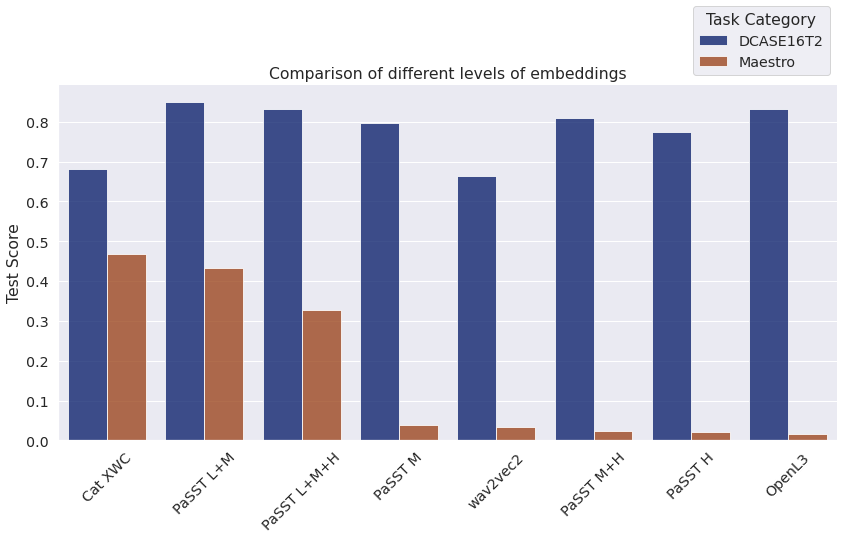
Figure 4: Comparison of different levels of extracted representations for PaSST models with hop=10 ms and receptive field size of 160 ms.

Two tasks in HEAR 2021, DCASE 2016 Task 2 and MAESTRO, rely on timestamp embeddings. We compare changes in our setup that effect timestamp embeddings with two single models, OpenL3 (Cramer et al., 2019) and Wav2Vec2 (Baevski et al., 2020), as well as the best performing submission to HEAR 2021 in the MAESTRO task, named Cat XWC, as a reference. OpenL3 is trained in a self-supervised way using the audio and videos of Audioset. Cat XWC is a concatenation of three diverse models: (1) HuBERT (Hsu et al., 2021) which is a self-supervised approach for speech representation learning, (2) wav2vec2(Baevski et al., 2020) is another model pre-trained on speech tasks (3) CREPE (Kim et al., 2018b) which is a specialized pitch estimation model.

5.1.1 Adding Low-Level Features

Figure 4 shows that including low-level embeddings (L+M and L+M+H) outperforms approaches with other combinations on the MAESTRO task while maintaining a high performance on the DCASE task. Models that do not include the low-level features fail to achieve a high score on the MAESTRO task, which means that the mid- and high-level representations extracted by PaSST do not convey relevant information for the music-related MAESTRO task.

5.1.2 Receptive Field

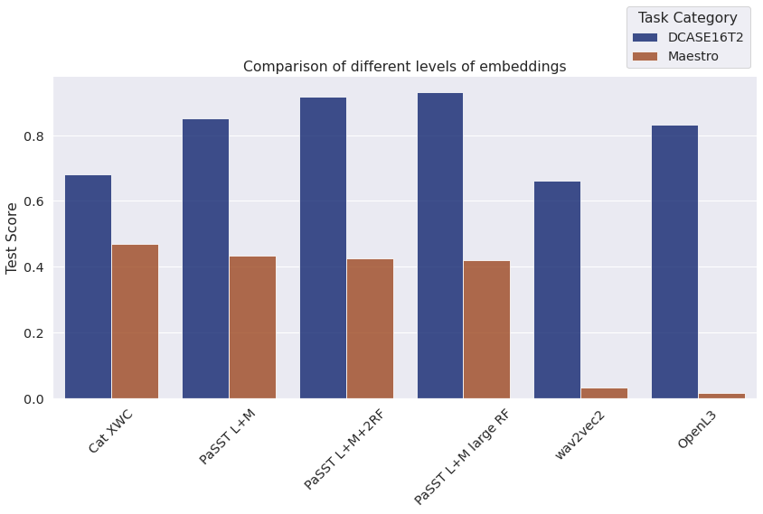
Figure 5: Comparison of different receptive field (RF) sizes of PaSST L+M models with hop=10 ms. The base model has RF=160 ms, large RF=640 ms. 2RF indicates concatenating the embedding of both receptive fields.

Figure 5 compares PaSST L+M models with small RF=160 ms, large RF=640 ms and concatenation of both (2RF). The results show that models with larger RF perform much better on the DCASE task while nearly maintaining their performance on the Maestro task.

5.2 Using Mid- and High-level Features

Figure 6: The effect of using different levels of PaSST representations as embeddings. Three different settings are compared: only mid-level M, only high-level H (MLP logits), and concatenating mid- and high-level representations M+H.

Figure 6 compares using medium- and high-level features as embeddings. Using only mid-level features produces the best results across all categories; concatenating mid- and high-level features yields similar results; and using only high-level features yields the worst results. This suggests that the high-level features of the output PaSST’s MLP classifier (see Section 4.1) generalize less because they contain very specific information about Audioset classes. This is demonstrated by the greatest drop in performance in speech tasks that are the furthest away from Audioset classes, as well as music tasks that are further away than the general category. The mid-level features provide a more abstract representation of the audio, which is beneficial for downstream tasks.

5.3 Using Finer Temporal Resolution

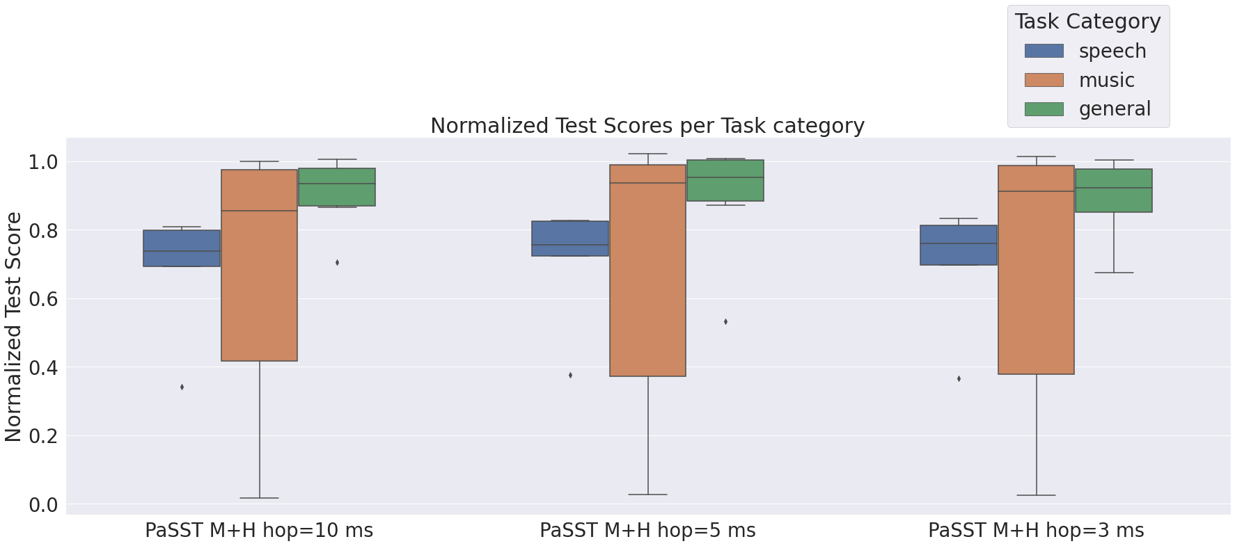
Figure 7: The impact of varying the temporal resolution by changing the hop-size of the STFT window on PaSST performance.

STFT hop	Seq. / P	Speed / P	P Speedup	Infer.	Audioset
10ms	1190 / 474	23.1 / 88.7	$3.8\times$	62.5	47.6
5ms	2388 / 594	6.8 / 62.4	$9.2\times$	18.9	47.3
3ms	3828 / 1014	3 / 29.7	$9.9\times$	8.5	47.3

Table 2: Changing the temporal resolution of PaSST. Seq.: indicates the input sequence length to attention layers. P: With Patchout. Speed: 10-second-audio training samples per second on an Nvidia Titan RTX GPU. Infer.: Inference speed in samples per second. Audioset: Supervised performance on Audioset in mean Average Precision (mAP).

We trained variants with a finer temporal resolution by decreasing the STFT hop size from 10 ms to 5 ms and 3 ms (as explained in Section 4.2). As can be seen in Figure 7, the model with a hop size of 5 ms improves the results for the categories general and speech, and marginally for the category music. Reducing the hop size even further to 3 ms does not result in additional improvements for any category, but instead worsens the results. Overall, environmental sounds and especially speech benefit from a higher temporal resolution compared to the base PaSST model. However, this higher resolution comes with a large complexity increase, as shown in Table 2.

5.4 Single Model Analysis

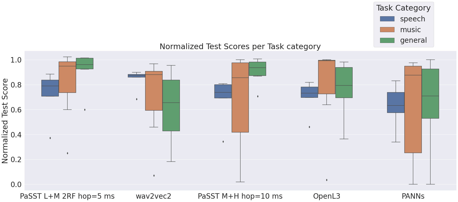
Figure 8: The figure shows a comparison of the models OpenL3 (Cramer et al., 2019), Wav2Vec2 (Baevski et al., 2020), PANNs (Kong et al., 2020), PaSST (Koutini et al., 2022) in its baseline setting and the improved PaSST model. The y-axis depicts normalized test scores per task. Each model is evaluated by three boxplots for the task categories general, speech, and music.

Figure 8 compares different single models on the HEAR categories (see Table 1). OpenL3 (Cramer et al., 2019) and PANNs (Kong et al., 2020) are based on CNN architectures. PaSST is a transformer model. Wav2Vec2 (Baevski et al., 2020) is a 1D-CNN with a positional transformer. PANNs and PaSST are trained on Audioset. OpenL3 is trained on both the audio and video of Audioset in a self-supervised way. Wav2Vec2 is trained in self-supervised fashion on 100K hours of speech from VoxPopuli (Wang et al., 2021). On the speech tasks, Figure 8 shows that the specialized model Wav2Vec2 outperforms the models trained on Audioset, PaSST base scores better on average than OpenL3 and PANNs. On music tasks, the distribution of scores has a large variance. OpenL3 shows the best performance. In the general category, PaSST base results in the best performance scoring between 90% and 100% of the best scoring models in the challenge in each task. Comparing CNNs (PANNS) and transformers (PaSST) trained on the same dataset, Figure 8 shows that the embeddings from PaSST score better in all categories. Figure 8 additionally shows an improved version of PaSST with the hyper-parameter settings that turned out to be beneficial in the preceding sections. The improved PaSST version (L+M 2RF hop=5ms) scores better in all categories compared to its baseline version. In particular, scores in the music category are improved and have less variance.

6 Conclusion

In this paper, we examine different approaches to extract general audio representations using the PaSST transformer model, which was pre-trained on Audioset. Compared to CNNs trained on the same dataset, our results show that representations extracted by the transformers are more general and capture information that can be better transferred to other tasks. Despite the variety of Audoiset classes, the results show that mid-level features are more general than high-level logits and can better transfer to downstream tasks. Finally, we highlight the trade-off between performance and computational complexity that arises when the temporal resolution is changed.

A Training Setup

We use the same download and pre-processing of YouTube Audioset videos as PANNs (Kong et al., 2020), resulting in approximately 2 million 10-second mono audio clips with a sampling rate of 32 Khz. Therefore, we use resampled version to 32Khz of the HEAR 21 datasets (Turian et al., 2022). The default Mel feature parameters are similar to those of AST; we use a $25$ ms window for Short-Time Fourier Transform (STFT) with a hop length of $10$ ms, resulting in $128$ mel bands and a $1000$ time frames. As explained in Section 4.2, we also look into finer time resolution using shorter hop lengths. We balance the training set as explained in Koutini et al. (2022). The reported results on Audioset are evaluated on $18,951$ audio clips. We use the AdamW (Loshchilov and Hutter, 2019) optimizer with a weight decay of $10^{-4}$, with a learning rate of $10^{-5}$ and a scheduler as explained Koutini et al. (2022).

All the used models are based on DeiT B↑384 (Touvron et al., 2021) pretrained on ImageNet (Deng et al., 2009) as proposed by Gong et al. (2021). For models with an STFT window hop of 10 ms, we use structured Patchout (see Section 2.2) to remove 4 rows (the frequency dimension) and 40 columns (the time dimension). For the models with hops of 5ms and 3ms, we remove 6 rows and 100, 150 columns, respectively. As a result, the sequence lengths and training speedups shown in table 2 were achieved.

As explained in Koutini et al. (2022), we use a number of data augmentations, including Mix-up (Zhang et al., 2018), SpecAugment (Park et al., 2019), waveform rolling, and random Gain

B Extended Model Comparison

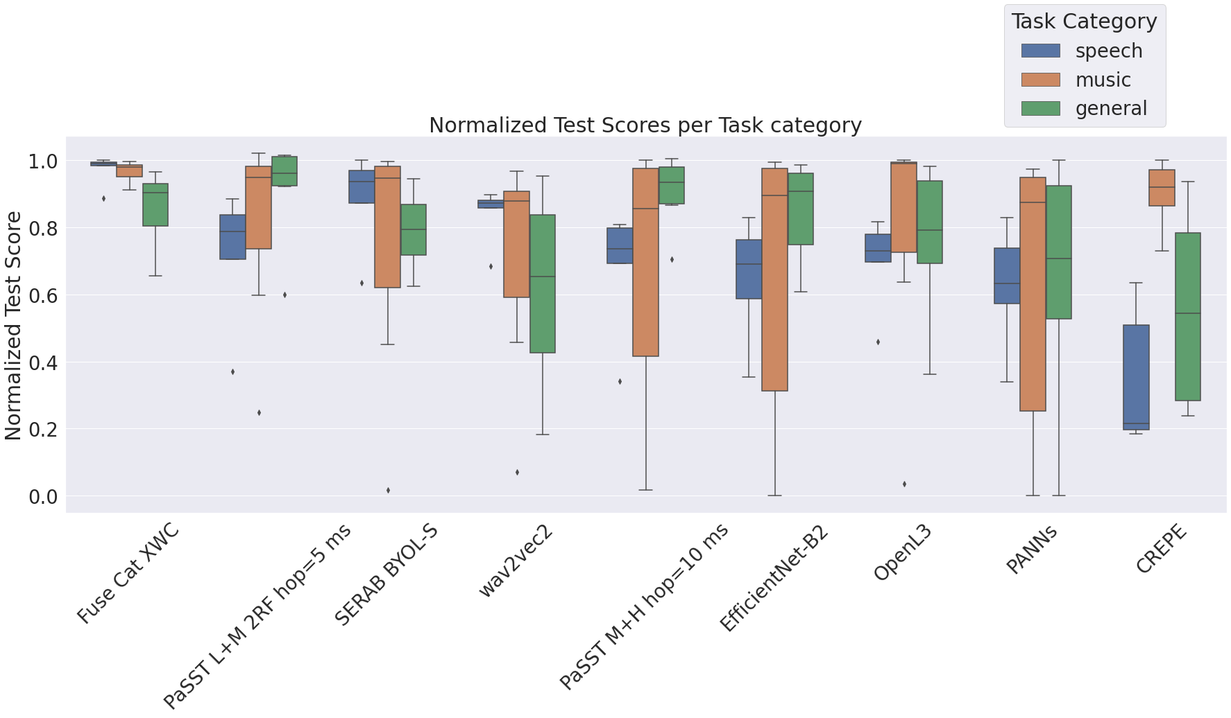
Figure 9: Comparing models that participated in the HEAR 2021 challenge with PaSST L+M 2RF hop=5 ms, which is a PaSST model equipped with better hyper-parameter settings for representation extraction (using the results from Section 5).

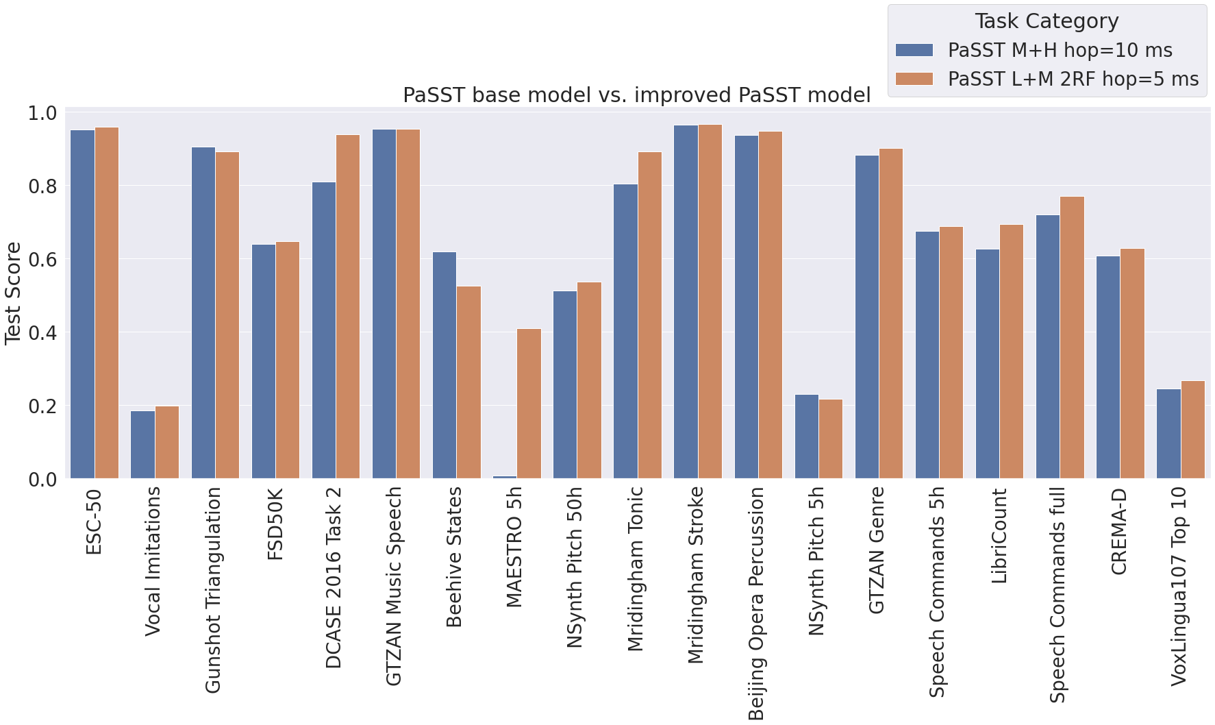
Figure 10: Comparing the results of the PaSST base model (submitted to the HEAR challenge) with the variant equipped with better hyper-parameter settings for representation extraction (using the results from Section 5).

Figure 9 compares different models that participated in the HEAR 2021 challenge (Turian et al., 2022). The models are sorted according to the median normalized test score across all tasks. With respect to this sorting Fuse Cat XWC, which is a combination of the three models HuBERT (Hsu et al., 2021), wav2vec2 (Baevski et al., 2020) and CREPE (Kim et al., 2018b).

Figure 10 highlights the performance gains resulting from using better hyper-parameter settings based on the results presented in Section 5. The figure compares the PaSST base model as submitted to the HEAR challenge PaSST M+H hop=10ms, with the improved version PaSST L+M 2RF hop=5ms on all the tasks.

References

- Abu-El-Haija et al. (2016) Sami Abu-El-Haija, Nisarg Kothari, Joonseok Lee, Paul Natsev, George Toderici, Balakrishnan Varadarajan, and Sudheendra Vijayanarasimhan. Youtube-8m: A large-scale video classification benchmark. CoRR, abs/1609.08675, 2016.
- Anantapadmanabhan et al. (2013) Akshay Anantapadmanabhan, Ashwin Bellur, and Hema A. Murthy. Modal analysis and transcription of strokes of the mridangam using non-negative matrix factorization. In IEEE International Conference on Acoustics, Speech and Signal Processing, ICASSP 2013, Vancouver, BC, Canada, May 26-31, 2013, pages 181–185. IEEE, 2013. doi: 10.1109/ICASSP.2013.6637633.
- Arandjelovic and Zisserman (2017) Relja Arandjelovic and Andrew Zisserman. Look, listen and learn. In IEEE International Conference on Computer Vision, ICCV 2017, Venice, Italy, October 22-29, 2017, pages 609–617. IEEE Computer Society, 2017. doi: 10.1109/ICCV.2017.73.
- Baevski et al. (2020) Alexei Baevski, Yuhao Zhou, Abdelrahman Mohamed, and Michael Auli. wav2vec 2.0: A framework for self-supervised learning of speech representations. In Advances in Neural Information Processing Systems 33: Annual Conference on Neural Information Processing Systems 2020, NeurIPS 2020, December 6-12, 2020, virtual, 2020.
- Cao et al. (2014) Houwei Cao, David G. Cooper, Michael K. Keutmann, Ruben C. Gur, Ani Nenkova, and Ragini Verma. Crema-d: Crowd-sourced emotional multimodal actors dataset. IEEE Transactions on Affective Computing, 5(4):377–390, 2014. doi: 10.1109/TAFFC.2014.2336244.
- Cooper and Shaw (2020) Seth Cooper and Steven Shaw. Gunshots recorded in an open field using ipod touch devices. Dryad, Dataset, 2020. doi: 10.5061/dryad.wm37pvmkc.
- Cramer et al. (2019) Jason Cramer, Ho-Hsiang Wu, Justin Salamon, and Juan Pablo Bello. Look, listen, and learn more: Design choices for deep audio embeddings. In IEEE International Conference on Acoustics, Speech and Signal Processing, ICASSP 2019, Brighton, United Kingdom, May 12-17, 2019, pages 3852–3856. IEEE, 2019. doi: 10.1109/ICASSP.2019.8682475.
- Deng et al. (2009) Jia Deng, Wei Dong, Richard Socher, Li-Jia Li, Kai Li, and Li Fei-Fei. Imagenet: A large-scale hierarchical image database. In 2009 IEEE Computer Society Conference on Computer Vision and Pattern Recognition (CVPR 2009), 20-25 June 2009, Miami, Florida, USA, pages 248–255. IEEE Computer Society, 2009. doi: 10.1109/CVPR.2009.5206848.
- Devlin et al. (2019) Jacob Devlin, Ming-Wei Chang, Kenton Lee, and Kristina Toutanova. BERT: pre-training of deep bidirectional transformers for language understanding. In Proceedings of the 2019 Conference of the North American Chapter of the Association for Computational Linguistics: Human Language Technologies, NAACL-HLT 2019, Minneapolis, MN, USA, June 2-7, 2019, Volume 1 (Long and Short Papers), pages 4171–4186. Association for Computational Linguistics, 2019. doi: 10.18653/v1/n19-1423.
- Dosovitskiy et al. (2021) Alexey Dosovitskiy, Lucas Beyer, Alexander Kolesnikov, Dirk Weissenborn, Xiaohua Zhai, Thomas Unterthiner, Mostafa Dehghani, Matthias Minderer, Georg Heigold, Sylvain Gelly, Jakob Uszkoreit, and Neil Houlsby. An image is worth 16x16 words: Transformers for image recognition at scale. In 9th International Conference on Learning Representations, ICLR 2021, Virtual Event, Austria, May 3-7, 2021. OpenReview.net, 2021.
- Engel et al. (2017) Jesse Engel, Cinjon Resnick, Adam Roberts, Sander Dieleman, Douglas Eck, Karen Simonyan, and Mohammad Norouzi. Neural audio synthesis of musical notes with wavenet autoencoders, 2017.
- Fonseca et al. (2022) Eduardo Fonseca, Xavier Favory, Jordi Pons, Frederic Font, and Xavier Serra. FSD50K: an open dataset of human-labeled sound events. IEEE/ACM Transactions on Audio, Speech, and Language Processing, 30:829–852, 2022. doi: 10.1109/TASLP.2021.3133208.
- Gemmeke et al. (2017) Jort F. Gemmeke, Daniel P. W. Ellis, Dylan Freedman, Aren Jansen, Wade Lawrence, R. Channing Moore, Manoj Plakal, and Marvin Ritter. Audio set: An ontology and human-labeled dataset for audio events. In 2017 IEEE International Conference on Acoustics, Speech and Signal Processing, ICASSP 2017, New Orleans, LA, USA, March 5-9, 2017, pages 776–780. IEEE, 2017. doi: 10.1109/ICASSP.2017.7952261.
- Gong et al. (2021) Yuan Gong, Yu-An Chung, and James R. Glass. AST: audio spectrogram transformer. In Interspeech 2021, 22nd Annual Conference of the International Speech Communication Association, Brno, Czechia, 30 August - 3 September 2021, pages 571–575. ISCA, 2021. doi: 10.21437/Interspeech.2021-698.
- Hawthorne et al. (2019) Curtis Hawthorne, Andriy Stasyuk, Adam Roberts, Ian Simon, Cheng-Zhi Anna Huang, Sander Dieleman, Erich Elsen, Jesse H. Engel, and Douglas Eck. Enabling factorized piano music modeling and generation with the MAESTRO dataset. In 7th International Conference on Learning Representations, ICLR 2019, New Orleans, LA, USA, May 6-9, 2019, 2019.
- Hershey et al. (2017) Shawn Hershey, Sourish Chaudhuri, Daniel P. W. Ellis, Jort F. Gemmeke, Aren Jansen, R. Channing Moore, Manoj Plakal, Devin Platt, Rif A. Saurous, Bryan Seybold, Malcolm Slaney, Ron J. Weiss, and Kevin W. Wilson. CNN architectures for large-scale audio classification. In 2017 IEEE International Conference on Acoustics, Speech and Signal Processing, ICASSP 2017, New Orleans, LA, USA, March 5-9, 2017, pages 131–135. IEEE, 2017. doi: 10.1109/ICASSP.2017.7952132.
- Hsu et al. (2021) Wei-Ning Hsu, Benjamin Bolte, Yao-Hung Hubert Tsai, Kushal Lakhotia, Ruslan Salakhutdinov, and Abdelrahman Mohamed. Hubert: Self-supervised speech representation learning by masked prediction of hidden units. IEEE/ACM Transactions on Audio, Speech, and Language Processing, 29:3451–3460, 2021.
- Humphrey et al. (2018) Eric Humphrey, Simon Durand, and Brian McFee. Openmic-2018: An open data-set for multiple instrument recognition. In Proceedings of the 19th International Society for Music Information Retrieval Conference, ISMIR 2018, Paris, France, September 23-27, 2018, pages 438–444, 2018.
- Kim et al. (2018a) Bongjun Kim, Madhav Ghei, Bryan Pardo, and Zhiyao Duan. Vocal imitation set: a dataset of vocally imitated sound events using the audioset ontology. In Proceedings of the Detection and Classification of Acoustic Scenes and Events 2018 Workshop, pages 148–152, 2018a.
- Kim et al. (2018b) Jong Wook Kim, Justin Salamon, Peter Li, and Juan Pablo Bello. Crepe: A convolutional representation for pitch estimation. In 2018 IEEE International Conference on Acoustics, Speech and Signal Processing, ICASSP 2018, Calgary, AB, Canada, April 15-20, 2018, pages 161–165. IEEE, 2018b. doi: 10.1109/ICASSP.2018.8461329.
- Kong et al. (2020) Qiuqiang Kong, Yin Cao, Turab Iqbal, Yuxuan Wang, Wenwu Wang, and Mark D. Plumbley. Panns: Large-scale pretrained audio neural networks for audio pattern recognition. IEEE/ACM Transactions on Audio, Speech, and Language Processing, 28:2880–2894, 2020. doi: 10.1109/TASLP.2020.3030497.
- Koutini et al. (2019a) Khaled Koutini, Hamid Eghbal-zadeh, Matthias Dorfer, and Gerhard Widmer. The Receptive Field as a Regularizer in Deep Convolutional Neural Networks for Acoustic Scene Classification. In 27th European Signal Processing Conference, EUSIPCO 2019, A Coruña, Spain, September 2-6, 2019, pages 1–5. IEEE, 2019a. doi: 10.23919/EUSIPCO.2019.8902732.
- Koutini et al. (2019b) Khaled Koutini, Hamid Eghbal-zadeh, and Gerhard Widmer. CP-JKU submissions to DCASE’19: Acoustic scene classification and audio tagging with receptive-field-regularized CNNs. Technical report, DCASE2019 Challenge, June 2019b.
- Koutini et al. (2021) Khaled Koutini, Hamid Eghbal-zadeh, and Gerhard Widmer. Receptive Field Regularization Techniques for Audio Classification and Tagging with Deep Convolutional Neural Networks. IEEE/ACM Transactions on Audio, Speech, and Language Processing, 29:1987–2000, 2021. doi: 10.1109/TASLP.2021.3082307.
- Koutini et al. (2022) Khaled Koutini, Jan Schlüter, Hamid Eghbal-zadeh, and Gerhard Widmer. Efficient Training of Audio Transformers with Patchout. In Interspeech 2022, 23nd Annual Conference of the International Speech Communication Association, pages 2753–2757. ISCA, 2022. doi: 10.21437/Interspeech.2022-227.
- Lafay et al. (2017) G. Lafay, E. Benetos, and M. Lagrange. Sound event detection in synthetic audio: Analysis of the DCASE 2016 task results. In 2017 IEEE Workshop on Applications of Signal Processing to Audio and Acoustics (WASPAA), pages 11–15, Oct 2017. doi: 10.1109/WASPAA.2017.8169985.
- Loshchilov and Hutter (2019) Ilya Loshchilov and Frank Hutter. Decoupled weight decay regularization. In 7th International Conference on Learning Representations, ICLR 2019, New Orleans, LA, USA, May 6-9, 2019. OpenReview.net, 2019.
- Nolasco et al. (2019) Inês Nolasco, Alessandro Terenzi, Stefania Cecchi, Simone Orcioni, Helen L. Bear, and Emmanouil Benetos. Audio-based identification of beehive states. In IEEE International Conference on Acoustics, Speech and Signal Processing, ICASSP 2019, Brighton, United Kingdom, May 12-17, 2019, pages 8256–8260. IEEE, 2019. doi: 10.1109/ICASSP.2019.8682981.
- Park et al. (2019) Daniel S. Park, William Chan, Yu Zhang, Chung-Cheng Chiu, Barret Zoph, Ekin D. Cubuk, and Quoc V. Le. Specaugment: A simple data augmentation method for automatic speech recognition. In Interspeech 2019, 20th Annual Conference of the International Speech Communication Association, Graz, Austria, 15-19 September 2019, pages 2613–2617. ISCA, 2019. doi: 10.21437/Interspeech.2019-2680.
- Piczak (2015) Karol J. Piczak. ESC: Dataset for Environmental Sound Classification. In Proceedings of the 23rd Annual ACM Conference on Multimedia, pages 1015–1018, Brisbane, Australia, October 2015. ACM Press. ISBN 978-1-4503-3459-4. doi: 10.1145/2733373.2806390.
- Plakal and Ellis (2022) Manoj Plakal and Daniel P. W. Ellis. YAMNet pretrained network. https://github.com/tensorflow/models/tree/master/research/audioset/yamnet, 2022. Accessed: 2022-02-21.
- Schneider et al. (2019) Steffen Schneider, Alexei Baevski, Ronan Collobert, and Michael Auli. wav2vec: Unsupervised pre-training for speech recognition. In Gernot Kubin and Zdravko Kacic, editors, Interspeech 2019, 20th Annual Conference of the International Speech Communication Association, Graz, Austria, 15-19 September 2019, pages 3465–3469. ISCA, 2019. doi: 10.21437/Interspeech.2019-1873.
- Srivastava et al. (2014) Nitish Srivastava, Geoffrey Hinton, Alex Krizhevsky, Ilya Sutskever, and Ruslan Salakhutdinov. Dropout: A simple way to prevent neural networks from overfitting. Journal of Machine Learning Research, 15(56):1929–1958, 2014. doi: 10.5555/2627435.2670313.
- Stöter et al. (2018) Fabian-Robert Stöter, Soumitro Chakrabarty, Bernd Edler, and Emanuël A. P. Habets. Classification vs. regression in supervised learning for single channel speaker count estimation. In 2018 IEEE International Conference on Acoustics, Speech and Signal Processing, ICASSP 2018, Calgary, AB, Canada, April 15-20, 2018, pages 436–440. IEEE, 2018. doi: 10.1109/ICASSP.2018.8462159.
- Tian et al. (2014) Mi Tian, Ajay Srinivasamurthy, Mark B. Sandler, and Xavier Serra. A study of instrument-wise onset detection in beijing opera percussion ensembles. In IEEE International Conference on Acoustics, Speech and Signal Processing, ICASSP 2014, Florence, Italy, May 4-9, 2014, pages 2159–2163. IEEE, 2014. doi: 10.1109/ICASSP.2014.6853981.
- Touvron et al. (2021) Hugo Touvron, Matthieu Cord, Matthijs Douze, Francisco Massa, Alexandre Sablayrolles, and Hervé Jégou. Training data-efficient image transformers & distillation through attention. In Proceedings of the 38th International Conference on Machine Learning, ICML 2021, 18-24 July 2021, Virtual Event, volume 139 of Proceedings of Machine Learning Research, pages 10347–10357. PMLR, 2021.
- Turian et al. (2022) Joseph Turian, Jordie Shier, Humair Raj Khan, Bhiksha Raj, Björn W. Schuller, Christian J. Steinmetz, Colin Malloy, George Tzanetakis, Gissel Velarde, Kirk McNally, Max Henry, Nicolas Pinto, Camille Noufi, Christian Clough, Dorien Herremans, Eduardo Fonseca, Jesse Engel, Justin Salamon, Philippe Esling, Pranay Manocha, Shinji Watanabe, Zeyu Jin, and Yonatan Bisk. Hear: Holistic evaluation of audio representations. In Douwe Kiela, Marco Ciccone, and Barbara Caputo, editors, Proceedings of the NeurIPS 2021 Competitions and Demonstrations Track, volume 176 of Proceedings of Machine Learning Research, pages 125–145. PMLR, 06–14 Dec 2022.
- Tzanetakis and Cook (2002) G. Tzanetakis and P. Cook. Musical genre classification of audio signals. IEEE Transactions on Speech and Audio Processing, 10(5):293–302, 2002. doi: 10.1109/TSA.2002.800560.
- Valk and Alumäe (2021) Jörgen Valk and Tanel Alumäe. VOXLINGUA107: A dataset for spoken language recognition. In IEEE Spoken Language Technology Workshop, SLT 2021, Shenzhen, China, January 19-22, 2021, pages 652–658. IEEE, 2021. doi: 10.1109/SLT48900.2021.9383459.
- Vaswani et al. (2017) Ashish Vaswani, Noam Shazeer, Niki Parmar, Jakob Uszkoreit, Llion Jones, Aidan N. Gomez, Lukasz Kaiser, and Illia Polosukhin. Attention is all you need. In Advances in Neural Information Processing Systems 30: Annual Conference on Neural Information Processing Systems 2017, December 4-9, 2017, Long Beach, CA, USA, pages 5998–6008, 2017.
- Wang et al. (2021) Changhan Wang, Morgane Rivière, Ann Lee, Anne Wu, Chaitanya Talnikar, Daniel Haziza, Mary Williamson, Juan Miguel Pino, and Emmanuel Dupoux. Voxpopuli: A large-scale multilingual speech corpus for representation learning, semi-supervised learning and interpretation. In Proceedings of the 59th Annual Meeting of the Association for Computational Linguistics and the 11th International Joint Conference on Natural Language Processing, ACL/IJCNLP 2021, (Volume 1: Long Papers), Virtual Event, August 1-6, 2021, pages 993–1003. Association for Computational Linguistics, 2021. doi: 10.18653/v1/2021.acl-long.80.
- Warden (2018) Pete Warden. Speech commands: A dataset for limited-vocabulary speech recognition. CoRR, abs/1804.03209, 2018.
- Zhang et al. (2018) Hongyi Zhang, Moustapha Cissé, Yann N. Dauphin, and David Lopez-Paz. mixup: Beyond empirical risk minimization. In 6th International Conference on Learning Representations, ICLR 2018, Vancouver, BC, Canada, April 30 - May 3, 2018, Conference Track Proceedings. OpenReview.net, 2018.