The American Put Option with A Random Time Horizon
Abstract
This paper is intended to provide a unique valuation formula for the American put option in a random time horizon; more precisely, such option restricts any stopping rules to be made before the last exit time of the price of the underlying assets at any fixed level. By exploiting the theory of enlargement of filtrations associated with random times, this pricing problem can be transformed into an equivalent optimal stopping problem with a semi-continuous, time-dependent gain function whose partial derivative is singular at certain point. The difficulties in establishing the monotonicity of the optimal stopping boundary and the regularity of the value function lie essentially in these somewhat unpleasant features of the gain function. However, it turns out that a successful analysis of the continuation and stopping sets with proper assumption can help us overcome these difficulties and obtain the important properties that possessed by the free-boundary, which eventually leads us to the desired free-boundary problem. After this, the nonlinear integral equations that characterise the free-boundary and the value function can be derived. The solution to these equations are examined in details. ††The authors are greatly indebted to Professor Ben Goldys for very helpful discussions.
Key Words: Option pricing, last exit time, optimal stopping, free-boundary problem
1 Introduction
Consider a complete defaultable market, with only one stock and one bond whose processes follow the stochastic differential equations:
where is a standard Brownian motion started at zero under measure , is the interest rate and is the volatility coefficient. This is a risk neutral model so that the discounted stock price is a martingale under measure ; in other words, is the risk neutral measure.
Then there is this option with expiration date (which can be indefinitely long) that entitles its holders to sell one share of stock for dollars at any time during the time frame between its purchase time and its exercise time or the last time the stock price price at any fixed level (whichever comes first); otherwise, it becomes worthless. How much are you willing to pay for this option?
When a contingent claim is valued, it is conventional to assume that there is no risk that the counter-party will default, that is, the counter party will always be able to make the promised payment. However, this assumption is far less defensible in the non-exchange-traded (or over-the-counter) market and the importance of considering default risk in over-counter markets is recognised by bank capital adequacy standards, see [17, Page 300] for a detailed introduction of default risk. According to [11, Pages 188 and 190], the contract given above can be viewed as the defaultable American contingent claims, with its default time modelled by the last exit time and by assuming the default market is complete, such contract is hedgeable.
A new factor that lies at the heart of current work is the presence of the last exit time in the classic valuation of American contingent claim. For a solid introduction and background of last exit time that is not stopping time, we refer to [23, Chapter 8.2]. The most interesting feature of the last exit time is its involvement of “the knowledge of the future”, which suggests that this work is closely related to the optimal prediction problem, see [2, 13, 16, 18] where this problem is also known as the stopping rule problem, the secretary problem and the optimal selection problem; and for the more recent work, see [9, 10]. For some financial applications of this factor that are remotely relevant to this work, we refer to the monographs [1, 11, 12].
With the aid of the classic pricing theory, the pricing problem posed above can be formulated into a precise mathematical form:
| (1.1) |
where is the exercise time, is the last exit time and is the strike price. Additionally, we assume that . By invoking the theory of enlargements of filtrations studied by Mansuy and Yor [22] and Nikeghbali [23], problem (1.1) can be further reduced to an equivalent optimal stopping problem without the presence of last exit time; for which, the classic method proposed in [24] can be partially applied. The resulting gain function in the finite-time formulated problem is semi-continuous, time-dependent with its partial derivatives being singular at certain point.
From the perspective of present work, the argument particularly consistent to the main result presented here is that by Peskir and Shiryaev [24]. Their work is able to provide a rather systematic methodology in a step-by-step fashion to tackle a wide range of optimal stopping problem associated with the American contingent claim valuation. Other useful references are [10, 9, 14]. In particular, the time-dependent reward problem was also studied in DuToit, Peskir and Shiryaev [10, 9], Glover, Peskir and Samee [14]. A somewhat different approach to verify the regularity the optimal stopping boundary was developed by De Angelis [4]. A treatment of the falling-apart smooth-fit condition was given by Qiu [28], Detemple and Kitapbayev [7].
The remainder of this paper is organised as follows: Section 2 is based on the published paper [15] of the author and the result presented here contains extension by considering the payoff of conventional contingent claim. This section covers the solution for problem (1.1) as . We begin by formulating the optimal stopping problem and its associated free-boundary problem in the form of ODE. After solving the ODE, we also proves its solution to be the smallest superharmonic function that dominates the gain function in Subsection 3.2. The heart of this paper is Section 3 which contains the unique pricing formula in Theorem 3.39 for the option posed above. Furthermore, being confronted with the singularity of the partial derivative, it becomes challenging to justify the regularity of value function and the optimal stopping boundary. As a result of this, one can only derive the semi-continuity of the value function first; but fortunately, this is just enough to confirm the existence of the optimal stopping rule in Lemma 3.7. The next focal point of this section is once again to justify the monotonicity of the boundary, which shall pave the way for us to address the problems caused by the singularity and then show the regularity of the value function and the boundary. To achieve this, the first thing we have to do is to pinpoint the stopping set by two crucial observations in Lemma 3.11 and Lemma 3.22 respectively: (i) the relative position of the free-boundary for pricing the American put option (which we take for granted) and the fixed level and (ii) the maximum of the gain function for any fixed time. Based on these observations and Assumption 3.26 concerning the choice of parameters in problem (1.1), we are able to present the monotonicity of the boundary in Proposition 3.17 and Proposition 3.34.
2 In the Infinite-time Horizon
2.1 Reformulation and Basics
In this subsection, we reformulate our main optimal stopping problem and prove some basic facts. By smoothing lemma and the measurability of stopping time ,
| (2.2) |
Next in line is the result of the Azéma supermartingale but first for notational convenience, we set and .
Proposition 2.1.
Let be the Azéma supermartingales associated with the random times . Then,
Proof.
As before, the set equality suggests that
so that
where the last equality follows via the general result in [30, Page 759 and 760]. ∎
Combining the above computation, the original problems (2.2) can be rewritten as
| (2.3) |
and for the sake of brevity, we denote the gain function .
Let us end this subsection by a useful property possessed by function .
Proposition 2.2.
The function satisfies the following ordinary differential equation, for ,
| (2.4) |
Proof.
Remember that the Doob-Meyer decomposition of the Azéma supermartingale is given by
| (2.5) |
and the measure is carried by the set .
Remark 2.3.
An alternative is to compute the first and second derivative of the function directly. Admittedly, the above proof is more clumsy than direct computation, but latter, as we shall see in the setting of finite time, the method of using Doob-Meyer decompostion is far more convenient.
2.2 The Free-boundary Problems
This subsection is devoted to formulating the free-boundary problem, whose solution will also be provided and verified.
The point of departure is to appeal to the local time-space formula (see [26]) as is of class on and obtain
| (2.6) |
where and are the local time of at the levels , respectively, and for brevity, we denote the martingale term as
Now, with a little bit of effort, we can compute:
and
so that (2.6) is reshuffled accordingly as
so that
| (2.7) | ||||
Immediate from (2.7), we see that the further gets away from the less likely that the gain will increase upon continuing, and this suggests that there exists a point such that the stopping time
| (2.8) |
is optimal for problem (2.3), with the convention that the infimum of the empty set is infinite. The optimality of will be verified in section 5.1.3.
The next logical task is, of course, to determine whether or not such stopping time is finite.
Corollary 2.4.
The stopping time is finite, i.e. .
Proof.
To verify for all , it suffices to show that .
With appeal to general result from [30, Page 759-760], we find that
where the third equality holds true as . Hence, for (i.e. ), by the assumption that , we have
which, joining with the fact that implies , shows that for all . ∎
With the aid of the above observations and the standard arguments based on the strong Markov property, we are now ready to formulate the free boundary problem to find the smallest superharmonic function that dominates and the unknown point ,
| (2.9) | |||
| (2.10) | |||
| (2.11) | |||
| (2.12) | |||
| (2.13) |
where is the infinitesimal generator of the strong Markov diffusion process .
Remark 2.5.
Another message of the free-boundary problem is that the optimal stopping level depends on the relative positions of the level .
We now proceed to solve the free-boundary problem. Equation (2.9) is the well-known Cauchy-Euler equation, whose solution gets form as follows
| (2.14) |
Then, by putting (2.14) into (2.9), we have the following quadratic equation
whose roots equal
from which, we know that the general solution of (2.9) is
where and are undetermined constants and by noticing that, in fact, for all , function , implying that must be zero.
By inspecting (2.10) and (2.11), we see that they are of different forms as and ,
| (2.15) |
and
| (2.16) |
and we have rediscovered Remark 2.5, from which, determining is within easy reach:
With a little additional effort, we work out the math for by using (2.11):
| (2.17) |
Remark 2.6.
Notice that, if , i.e. , then the result of standard perpetual American put option emerges.
The conclusion runs as follows:
Theorem 2.7.
Proof of Solution (2.18).
We wish to prove that in (2.2) equals in (2.15) for all , to achieve which, we proceed via three steps (proving three statements):
(i) for all . To prove this, we set
Knowing that for all reduces our task to verifying that in the domain . By rearrangement, we have
which yields that , and thereby proving statement (i).
(ii) for all . By invoking the local time-space formula, we obtain
| (2.20) |
where the second equality holds via the smooth-fit condition (2.11). Since for all such that
which, together with (2.9), tells us that
| (2.21) |
and then, immediate from statement (i) and (2.21) for all , we see that
| (2.22) |
Let for and then we know that, for every bounded stopping time of , taking the expectation under measure yields so that
Next, let , by Fatou’s lemma, . After this, by taking the supremum over all the stopping times of ,
| (2.23) |
and the desired statement (ii) follows.
(iii) for all . Put for in (2.20), with being the finite stopping time defined in (2.8),
and then by taking its expectation under measure , we have so that
Let , via an appeal to the dominated convergence theorem and the fact that , we see that
| (2.24) |
which yields statement (iii). Finally, combining (2.23) and (2.24) completes the proof. ∎
Remark 2.8.
The above proof is the same as showing that is the smallest superharmonic function that dominates : step (i) shows the domination, step (ii) we have being superharmonic function because of inequality (2.22) and (2.24) in step (iii) tells us that is the smallest superharmonic function that dominates . Therefore, is indeed optimal given that it is finite almost surely. See [24, Page 40, Theorem 2.7] for more details.
Proof of Solution (2.19).
Similar argument works for this solution, but since solution (2.19) is not differentiable on , which should require extra care in the following part of step (ii):
| (2.25) |
where the second equality holds via the smooth-fit condition and the inequality follows via . Since for all such that
which, together with (2.9), tells us that . This, combining with statement (i) yields . The rest of the proof follows similarly as the proof of (2.18). ∎
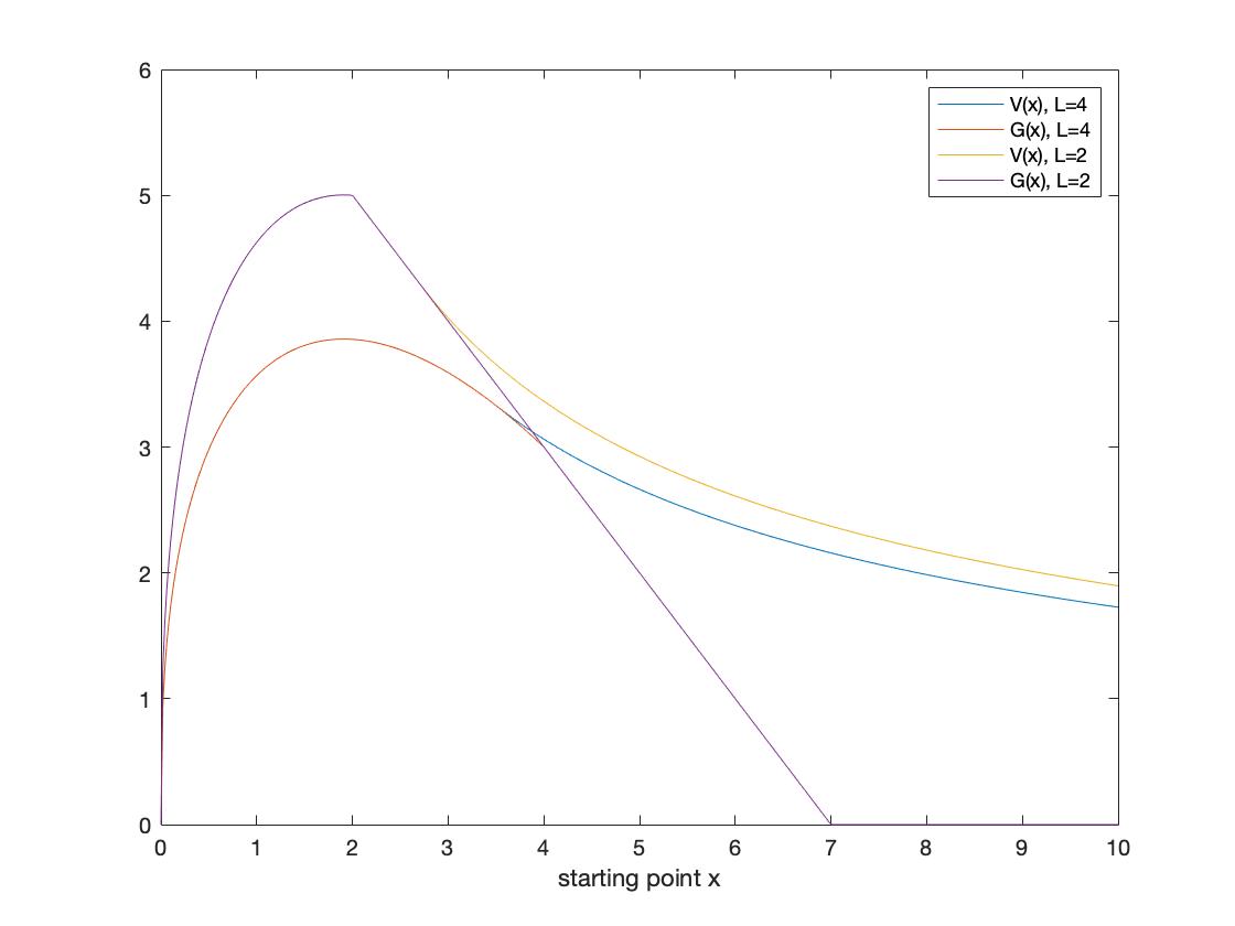
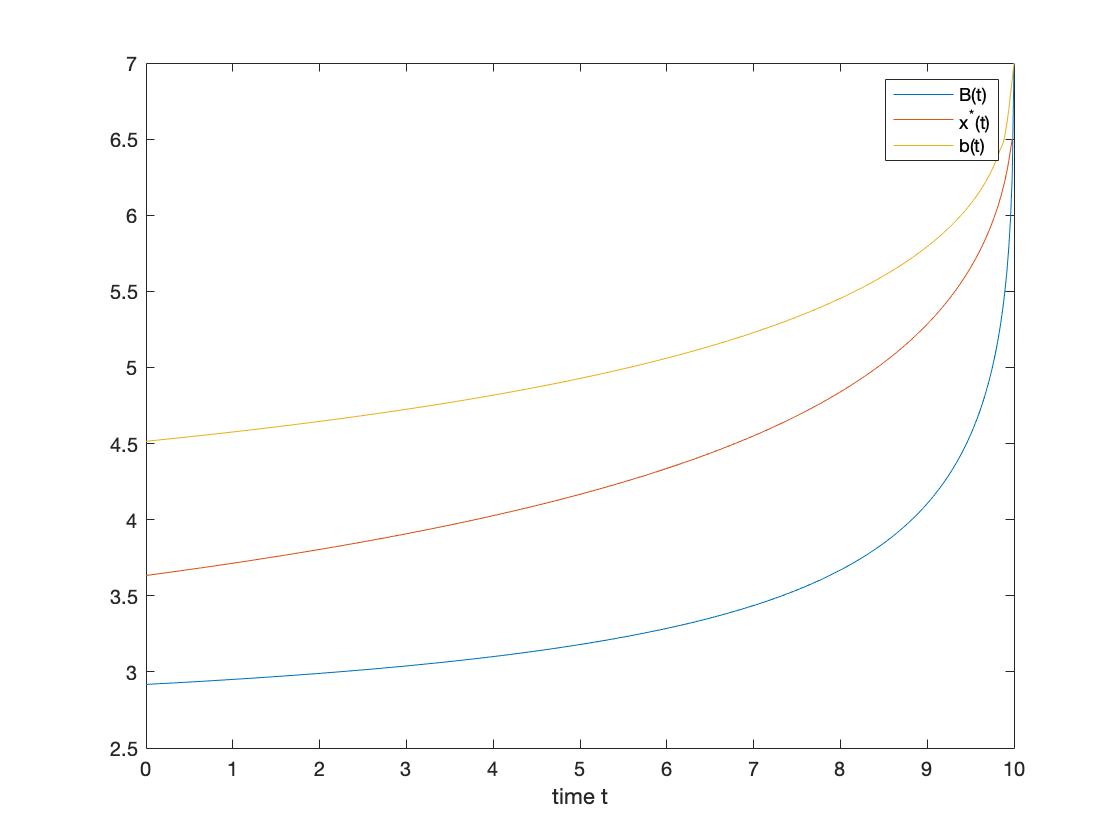
Remark 2.9.
Figure 1 shows that the value of perpetual contract is a decreasing function of , and is bounded above by the global maximum of and below by .
3 In the Finite-time Horizon
3.1 Reformulation and Basics
In this subsection, we once again reformulate problem (1.1) and collect some elementary facts that will be used later.
By the measurability of stopping time , we see that
| (3.26) |
The process is a strong Markov (diffusion) process with the infinitesimal generator given by
In the view of (3.26), the first thing is, of course, to calculate and let us introduce the notation,
where and .
Proposition 3.1.
Let be the Azéma supermartingale associated with the random time . Then, for and , for
Proof.
First of all, suppose that
where the second equality follows from the Markov property of and for easy reference, let
in plain language, is the first time when a geometric Brownian motion , starting from , hits the level .
Having introduced the Azéma supermartingale, the following facts are just around the corner.
Proposition 3.2.
The function satisfies the following partial differential equation, for ,
| (3.28) |
Proof.
Notice that direct computation is certainly an option, but making use of the Doob-Meyer decomposition shall be a much efficient way.
Let us apply the local time-space formula to obtain
| (3.29) |
where is the local time of at the level given by
after which, we can lean on the Doob-Meyer decomposition to conclude that
where is the cdlg martingale and is the predictable projection whose measure is carried by the set , and consequently, (3.28) follows. ∎
Corollary 3.3.
(i) The map is decreasing on ; (ii)The map is increasing on .
Summarising our findings so far, by the strong Markov property of , we can rewrite and generalise the original problem (3.26) as
| (3.30) |
and for simplicity, let the gain function .
3.2 The Free-boundary Problem
Before we turn to formulating the free-boundary problem, we squeeze the important concepts of continuation and stopping sets into the text.
Definition 3.4.
The continuation set and the stopping set are defined as follows:
| (3.31) | ||||
| (3.32) |
Based on the above definition, the first entry time of into is then defined as
| (3.33) |
It is then not far-fetched to ask for the optimality of , which, according to [24, Corollary 2.9, Page 46], is the same as showing the (semi)continuity of and .
Remark 3.5.
It is worth mentioning that (see (A.86)) has a singularity at point , so establishing the continuity of the value function can only be pursued later.
Lemma 3.6.
The value function is l.s.c on .
Proof.
As was noticed before, the supremum of an l.s.c function defined an l.s.c function, so we only have to establish the continuity (thereby l.s.c) of on and the assertion will follow immediately.
To achieve this, we begin by showing that (i) is continuous on for each . Take any in so that
where the first inequality is based on the map is decreasing, and first equality follows via the time-homogeneous property of GBM; after which, let , we see that by the dominated convergence theorem (function ),
and assertion (i) follows.
It remains to show that (ii) is continuous on for each . We simply observe that
where the third inequality follows from for ; after which, let , the monotone convergence theorem (it is applicable because of Corollary 3.3) suggests
By combining assertions (i) and (ii), the conclusion follows. ∎
With the aid of Lemma 3.6, we can then establish the optimality of . (See [24, Corollary 2.9, Page 46] for conditions of existence of the optimal stopping time.)
Lemma 3.7.
The stopping time is optimal in (3.30).
Proof.
Note that function is continuous (thereby u.s.c) on , which, together with Lemma 3.6, yield that
is optimal (with the convention that the infimum of the empty set is infinite) and in the following problem
so that , where its corresponding stopping set is defined as . Furthermore, observe that
which, together with Corollary 3.3, implies that
which implies that , and the desired claim follows. ∎
It will be shown in the next section that the continuation and stopping sets can be defined as
| (3.34) | |||
| (3.35) |
where is the unknown optimal stopping boundary such that can be rewritten as
| (3.36) |
and by Theorem 2.4 in [24, Page 37] and Corollary 3.7, the free-boundary problem can be formulated as:
| (3.37) | |||
| (3.38) | |||
| (3.39) | |||
| (3.40) | |||
| (3.41) |
3.3 The Continuation and Stopping Sets
As a further preparation for proceeding the detailed analysis, we lean on the local time-space formula, as the function is not differentiable and , to obtain
| (3.42) |
where and are the local times of at the level and respectively, and for simplicity, we denote the martingale term as
so that under measure for each .
A fairly easy calculation then shows that
and that, upon putting and using Proposition 3.2,
| (3.43) |
after which, (3.42) is reshuffled accordingly as
Remark 3.8.
Note how very nicely the property of function in Proposition 3.2 has saved us from massive computations in the finite-time problem setup!
Using this, we find that
| (3.44) |
from which, what intuition would suggest is the following:
Lemma 3.9.
All points belong to the continuation set .
Proof.
The proof follows, in fact, from verbal statement, since stopping at gives one null payoff, while waiting, there is a positive probability to collect strictly positive payoff. ∎
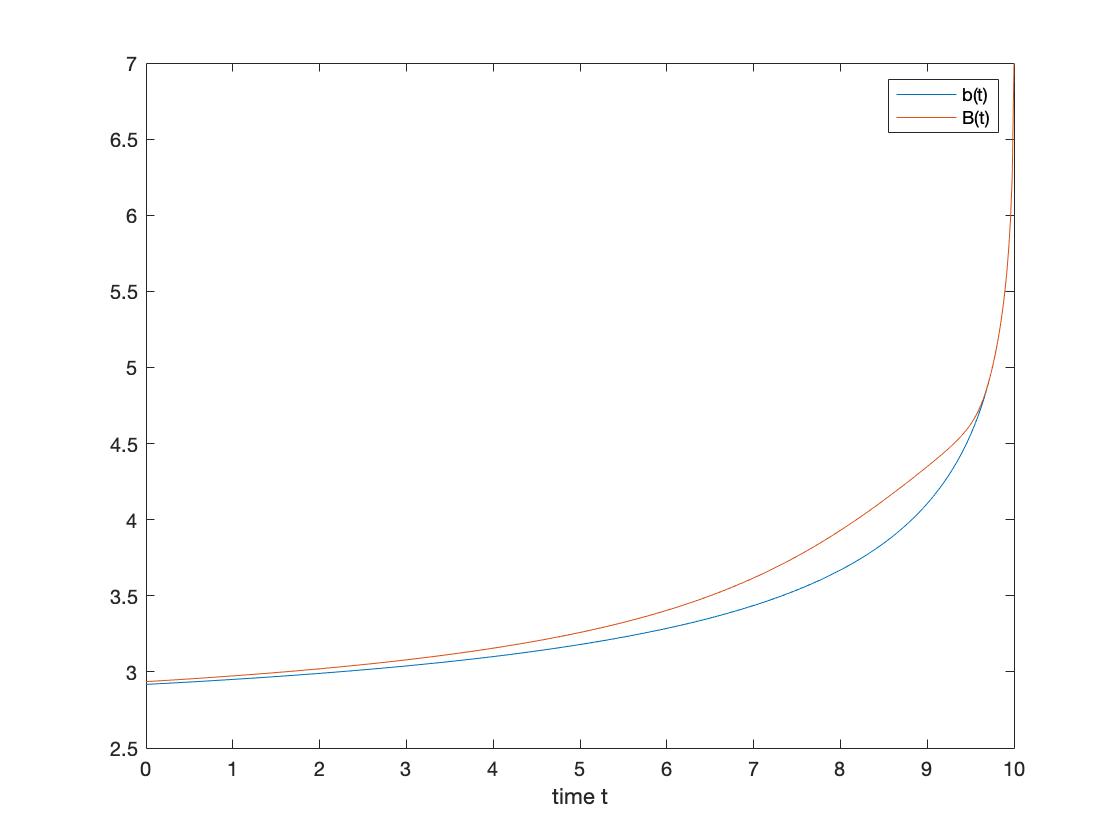
Remark 3.10.
For notational convenience, we let , and denote the value function, the gain function and the optimal stopping boundary for the standard American put option with the same maturity and strike price as the current contract. Then, we know from [24] that
where is unique and ; and thus, its stopping set and continuation set equal:
Also we define as follows:
and since the map is strictly increasing, is unique. Moreover, let us emphasise that , as .
Lemma 3.11.
All points belongs to the stopping set .
Proof.
Since , it follows from the construction of the stopping set for the standard American put option that
and notice that in this set, .
Now, knowing that
where the inequality is due to function being a probability and consequently,
on the set , which in the sense of forces the equation and thereby, proving the desired assertion. ∎
With a little additional work, we can extend Lemma 3.11 to the following result:
Lemma 3.12.
All points belongs to the stopping set .
Proof.
The proof amounts to showing that also belongs to the stopping set .
Lemma 3.11 tells us that . Suppose that we run the process starting at point , and we see from (3.44) that in order to compensate the negative term inside the expectation, the process shall hit level as the local time term is positive, but , indicating the process can not hit level before exercising at level . Therefore, it is optimal to stop immediately on this set and the conclusion follows. ∎
Remark 3.13.
With Remark 3.13 in mind, we now enter the discussions of the properties for sets and with and .
In the Case of , that is .
Proposition 3.14.
The stopping set is right-connected and the continuation set is left-connected.
Proof.
Let and consider the stopping time and suppose that is the optimal stopping time for so that , which is a consequence of Remark 3.13. Then, by the time-homogeneous property of GBM,
where the second equality follows from . This establishes the following relation:
from which, we see that implies and that implies . ∎
Proposition 3.15.
The stopping set is down-connected and the continuation set is up-connected.
We now have sufficient mathematics at our disposal to go around the singularity of for the establishment of the continuity of the value function for .
Lemma 3.16.
The value function is continuous on .
Proof.
The proof involves proving two assertions: (i) The map is continuous on for each given and fixed. Take any in , let and be the stopping time such that
Then, by setting , we have
and that
| (3.45) |
where the first inequality is because of the map being decreasing and the last inequality holds via
| (3.46) |
By letting , using and then on (3.45), the dominated convergence theorem allows us to conclude that
and assertion (i) follows.
(ii) The map is continuous on for each given and fixed.
Note that by the up-down connectedness of and , for any in ,
and let be optimal for such that
| (3.47) |
after which, by letting , the dominated convergence theorem leads us to
and thereby, proving the left-continuity of .
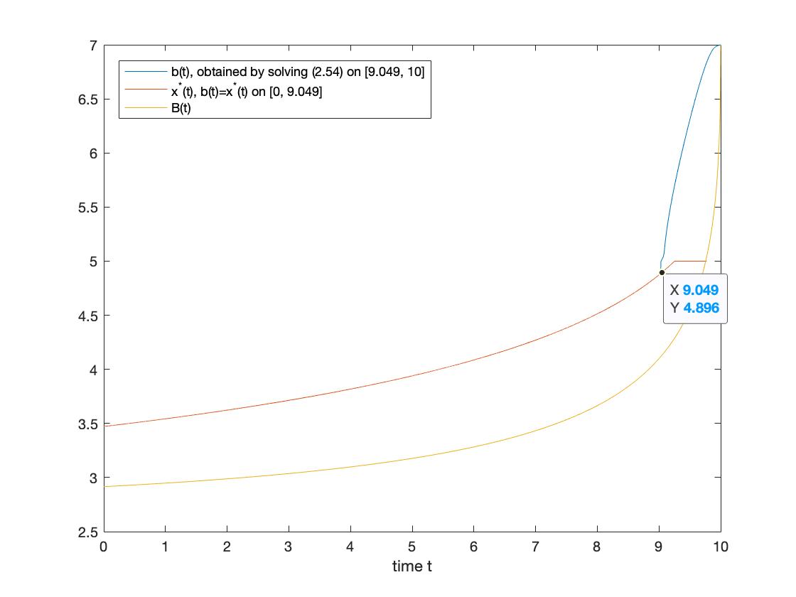
And, needless to say, if , Lemma 3.12 tells us that and the continuity of follows directly from that of the gain function .
On the other hand, if , we know there exists so that (see figure 2) and that for , immediately from the monotonicity of , we have
which implies a.s.; more precisely, by the strong solution of GBM and the optimality of , entails
and that for ,
after which, it follows that as for ,
and then by letting , we have , that is, the right-continuity of . By combining the claims that is left and right-continuous for for each given and fixed, statement (ii) follows. ∎
By taking advantage of the above analysis , we obtain the following result:
Proposition 3.17 (The Free-boundary Problem).
The stopping set and the continuation set are of the forms:
where the map is increasing.
The free-boundary problem is rearranged as follows:
| (3.48) | |||
| (3.49) | |||
| (3.50) | |||
| (3.51) | |||
| (3.52) |
Just to complete the picture of the free-boundary problem, we now justify equation (3.50).
Proof of the Smooth-fit Condition.
Let a point lying on the boundary be fixed, i.e. . Then, and for all such that , we have
of which, taking the limit as , we have .
In order to prove the converse inequality, we fix a sufficiently small so that and that , and consider the optimal stopping time for so that the monotonicity of tells us that implies almost surely, as before, by the strong solution of GBM,
so that, for ,
Then, we have
where the second inequality follows from
| (3.53) |
and the second equality is from the strong solution of and linearity; moreover, the fourth inequality is due to the fact that entails and that , while we used for chosen in the last step. Via an appeal to the dominated convergence theorem, upon letting , we have (see A.1 for its justification) so that
Thus,
after which, the conclusion follows via the fact that for and belong to ,
∎
Remark 3.18.
To prepare for the main theorem presented in Subsection 3.4, we further justify the continuity of the optimal stopping boundary.
Lemma 3.19.
The optimal stopping boundary is continuous on and .
Proof.
Th proof proceeds in three steps, which follows essentially from [24, Page 383].
(i) The boundary is right-continuous on .
Let us fix and take a sequence as . Since is increasing, the right-limit exists. Remember that is a closed set, meaning that its limit point is contained in , it then follows, together with the construction of the stopping set that . However, the fact that is increasing suggests that and thereby, forcing the equation and proving statement (i).
(ii) The boundary is left-continuous on .
Assume that, for contradiction, at some point , the function makes a jump, that is, . Then, fix a point . By (3.49) and (3.50), we have
| (3.54) |
for each , where and . Despite the fact that function is not differentiable at , the fact that once again comes to our rescue.
Knowing that the value function satisfies (3.48), we see that, for , where is a curved trapezoid formed by the vertices , , and ,
where the first strict inequality follows via the fact that both the maps and are decreasing on , and the last one is due to the fact that on . Moreover, on .
Then, from the continuity of the value function and the gain function, upon letting on (3.54) and using dominated convergence theorem,
which is a contradiction, since , indicating that such point cannot exist and must hold true. Immediate from statements (i) and (ii), the continuity of follows.
(iii) .
In Lemma 3.9, we learned that .
Assume that, so that there exists a point and let with . Then, by rerunning the proof of statement (ii) with the above modifications and letting , we find that from the continuity of and on ,
which contradicts the fact that and thus implies that (because of its continuity, ). ∎
In the Case of , that is .
Proposition 3.20.
On the state space , the stopping set is right-connected and the continuation set is left-connected.
Proof.
Since on the state space , the map is decreasing and that , the map is decreasing also. That is, for any , if , then
such that implies and implies , which is precisely the claim. ∎
Proposition 3.20 immediately tells us the following result, which we state without proof:
Corollary 3.21.
On the state space , .
To fill the last slot of the diagram, we shall show that the stopping set is not empty on state space , but first we present some important facts:
Lemma 3.22.
(i) The gain function is uniformly continuous on the state space ;
(ii) The map is continuous on .
(iii) Given that for each , is reached at a unique point , in particular,
| (3.55) |
the map is continuous on .
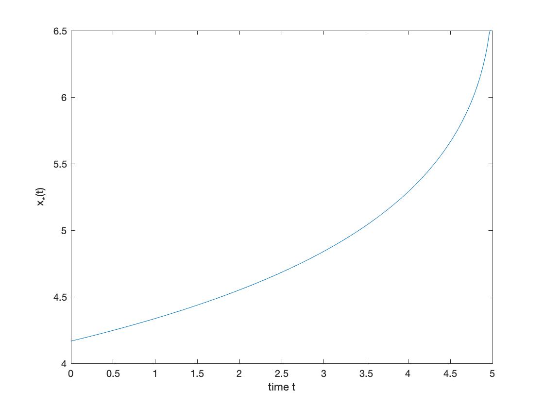
Remark 3.23.
Knowing from derivative computation that for each fixed , the maximum of G achieved in is the global maximum over the domain , we can write
As a matter of fact, is non-decreasing, see Figure 4.
Proof of Lemma 3.22 .
(i) To show that is uniformly continuous on , is to show that for every , there exists a so that for all , implies .
Notice that
Observe that on ,
where the second inequality holds true by the mean value theorem and the fact that the partial derivatives of and are bounded, say by constants and , on the set (see (A.85), (A.86)). Hence,
and we can now choose and verify that if satisfy , then
thus proving statement (i) as desired.
(ii) The uniform continuity of means that for every , there exists a such that for all and ,
which, after rearranging, equals
so we must have,
after which, the conclusion follows from
(iii) Assume that, for contradiction, statement (iii) is false. To say that, is not continuous on means that there exists a sequence where (Since the the set is compact, the limit point is always contained on .) such that does not converge .
According to statement (ii) and the definition of ,
but the assumption is
which is a contradiction, we may therefore conclude that statement (iii) holds true. ∎
What Lemma 3.22 tells us is that:
Lemma 3.24.
All points belongs to the stopping set .
Proof.
According to the definition of , Remark 3.23 and the fact that is decreasing,
and by domination, taking expectation under measure ,
so that , but forces the equation , and thus showing that all . Furthermore, due to Lemma 3.22 and Remark 3.23, an analogous argument as Lemma 3.12 does the rest for us. ∎
Remark 3.25.
It has been high-lighted in multiple literatures (if not all of them, such as [19, Page 113]) that if either the maps or are monotone (the later monotonicity is used to establish the up-connectedness of the sets), we will not be able to compare two integrals with different signs and proves most of the properties possessed by the optimal stopping boundary, which is probably the only downfall of such analytical method but opens the door to many interesting research possibilities; this is, unfortunately, the story of . By narrowing down the scale of the continuation set (the idea behind this is that, in the American put option pricing problem, the lower bound for the continuation set when is the optimal stopping level obtained from pricing the perpetual American put option), we can make an additional assumption to further develop some insights towards the shape of sets and .
Assumption 3.26.
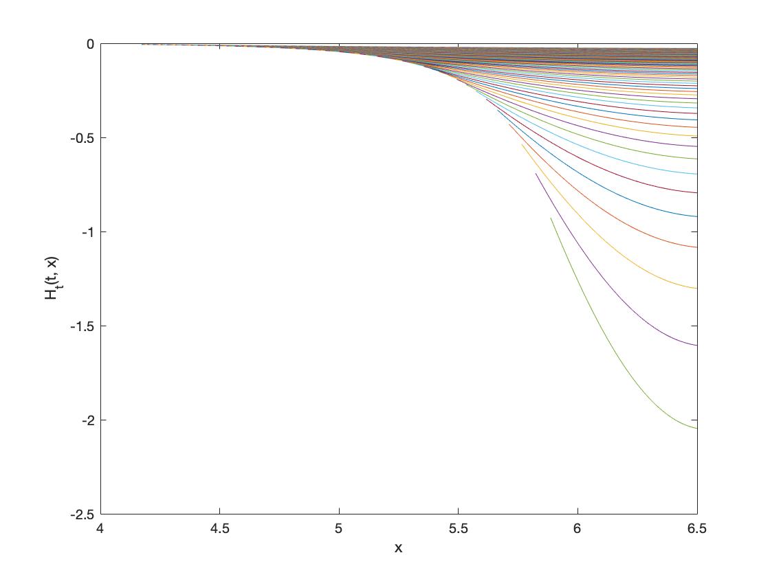
Parameters and can be chosen such that the map of is decreasing on the sets .
Remark 3.27.
Note that the above assumption holds true in the state space generally, see Figure 6. In addition, for , .
For future reference, set
so that .
Proposition 3.28.
The map is decreasing on .
Proof.
Let and consider the stopping times:
and be the optimal stopping time for , by the fact that , a direct result is . Then, we have
where the second inequality holds true via the map is decreasing and is increasing (see A). In particular, we have arrive at the inequality:
which is precisely the claim. ∎
The usefulness of Proposition 3.28 is well demonstrated by the following results:
Proposition 3.29.
(i) The stopping set is right-connected, i.e. increasing w.r.t time ;
(ii) The continuation set is left-connected, i.e. decreasing w.r.t time ;
(iii) The stopping set is down-connected;
(iv) The continuation set is up-connected.
Proof.
Assertions (i) and (ii) are immediate from Proposition 3.28, from which, (iii) and (iv) follow. ∎
Remark 3.30.
Once again, because the gain function is not smooth in the stopping set at level , the presence of the local-time term in the pricing formula should not come to us as a surprise; above all, the twist comes when the optimal stopping boundary is crossing or remaining for some time at (consider the situation for and for all , then ), the smooth-fit condition fails to hold. See [7, Page 19] for similar treatment of such problem.
Remark 3.31.
The minimal conditions under which the smooth-fit condition can hold in greater generality are the regularity of the diffusion process and the differentiability of the gain function . For further contribution and examples, we refer to [24, Page 155].
To further construct the continuity of the value function, we need a definition first:
Definition 3.32.
Let times and be defined as follows:
and if for all , we set . Note also that if , then .
As the reader has, hopefully noticed in the proof of Lemma 3.16 and Proposition 3.17, the difficulty in the proof of continuity of and smooth-fit condition lies in the singular point of (and thereby in the applicability of the dominated convergence theorem). To overcome this, the key idea is to keep the state space away from such a point by taking the continuity and the monotonicity of in into account (and these properties come for free!).
Lemma 3.33.
The value function is continuous on .
Proof.
The proof once again involves two statements, but with statement (i) of Lemma 3.16 remained unchanged, we confine ourselves by proving (ii) the map is continuous on for all . As before, the up-down connectedness of and suggests that for any in ,
and let be optimal for so that
| (3.56) |
in which, by letting , the dominated convergence theorem yields and thereby showing the left-continuity of w.r.t .
If for , Lemma 3.24 (see Figure 5) suggests that , which, together with the continuity of , shows that as . If, on the other hand, for , then
| (3.57) |
where the second inequality is because of inequality (3.46) and .
Before we proceed, recall that for (and ). By employing the continuity and monotonicity of , intermediate value theorem tells us that there exists so that and because , where (Set is the area coloured in green in Figure 5), we know that implies a.s. (see Figure 3), equation (3.57) therefore equals
| (3.58) |
where the last two steps are due to the mean value theorem for , the strong solution of GBM and the fact that in (see A.87).
Then, we can choose so that almost surely whenever and (the justification is the same as that in the proof of Lemma 3.16, we omit further details), by setting such in (3.58), joining with the fact that for ,
in which, let , we have , that is, is right continuous w.r.t . The conclusion follows as is right and left continuous for any for each given and fixed. ∎
To this point, we have been working really hard on the discussion of the stopping and continuation sets and now we can finally return to our main purpose, i.e. the formulation of free-boundary problem,
Proposition 3.34 (The Free-boundary Problem).
The stopping set and the continuation set are of the forms:
where the map is increasing. The free-boundary problem in section 2.2 is therefore reshuffled accordingly as
| (3.59) | |||
| (3.60) | |||
| (3.61) | |||
| (3.62) | |||
| (3.63) | |||
| (3.64) |
Proof of the Smooth-fit Condition (3.61).
The proof for is essentially the same as that of Proposition 3.17. It thus remains to show (3.61) holds true for . Let a point lying on the boundary be fixed, i.e. . Then, let such that , and
where the inequality is due to and ; of which, we take the limit as and obtain
| (3.65) |
In order to prove the converse inequality, we first note that (the exact same argument is presented in the proof of Lemma 3.33, so we omit some details here) there exists s.t. for . Then, let be optimal for , where we can choose so that almost surely whenever (the justification follows the same pattern as that in the proof of Lemma 3.16),
where the second inequality holds true because of (3.53) and the first equality follows from the facts that for of our choice, entails , the second equality is derived from the mean value theorem for . Recalling that the random variable is dominated by a positive integrable random variable, letting , a.s. and exploiting the dominated convergence theorem (the boundedness of for is verified in A.87) yield
| (3.66) |
which, together with (3.65) and the fact that so that
and this allows us to obtain (3.61). ∎
Proof of (3.62).
(i) Let such that there exists , and . The first part of (3.62) is a consequence of
and via letting , we see
(ii) Again, let so that there exists (where is defined as so that for ), and and that
Furthermore, let be the optimal stopping time for so that and that
where the second inequality is due to (3.53) and in the first equality, we use the fact that
and in the third equality, we apply mean value theorem for and with our choice of , entails a.s.; from which, we know that as , almost surely so that and hence, equations in (3.62) emerge. ∎
Before we bring this section to a close, we establish the continuity of the boundary.
Remark 3.35.
The proof of the continuity of on can be done by following the exact same pattern as that in Lemma 3.19, and if remains at level L in , we know from the left-connectedness of that during such amount of time, must be continuous. Our task has therefore been reduced to prove that is continuous on .
Lemma 3.36.
The optimal stopping boundary is continuous on and .
Remark 3.37.
The essential tool to prove Lemma 3.19 is the smooth-fit condition, which, may, at times, either be difficult to verify or hold true. Following is a rather convenient technique to prove the continuity based on the regularity of functions and and the monotonicity of .
Proof.
To avoid using smooth-fit condition, we use the argument provided in [4, Page 173-175].
(i) The boundary is right-continuous on . The conclusion is immediate from the fact that the stopping set is closed and is increasing on .
(ii) The boundary is left-continuous on . We assume that, for contradiction, there exists so that a discontinuity of occurs; that is, at , one has , where denotes the left limit of the boundary at , which always exists as is monotonically increasing in .
Let be fixed such that . Then, for fixed , we define an open bounded domain with . Hence, by the structure of , we know the value function , which is in , solves the Cauchy problem
| (3.67) |
Then, we denote as the set of function with infinitely many continuous derivatives and compact support in , in which, we define such that . By further multiplying (3.67) by function , and integrating the product over for some ,
| (3.68) |
where the second double integral on the left-hand side is strictly negative, as on . Therefore, we want to investigate the sign of first double integral by estimating its upper bound, which if is negative, the proof will be completed by reaching a contradiction. To do so, let us first observe that
| (3.69) |
where the inequality is the consequence of and .
Next in line is partial integrations (three times),
| (3.70) |
where, if we also impose the condition for the boundary terms disappear, is the formal adjoint of given as
Since ,
| (3.71) |
where are constants and , the first equality follows via again and the second inequality is due to the fulfilment of the conditions proposed on [4, Page 172, (C.3)].
In addition, we consider and set , upon using ,
of which, as a result, for any , in the view of (3.70),
| (3.72) |
where the last equality follows by partial integrations again.
Joining (3.69) with (3.72), from the view of equation (3.68),
| (3.73) | ||||
| (3.74) |
where the second inequality follows in the sense that in such interval , there exists some constant so that
and that ; since the second term in (3.73) is strictly positive, we can set
from which, the second equality holds.
Taking the limit thus leads to a contradiction in the sense that the second term on the last equality of (3.74) is vanishing more rapidly than its first term (that is, ), hence the jump may not occur. ∎
3.4 The Optimal Stopping Rule
In order to prepare for the main result, we shall first verify the conditions for the local time-space formula to be applicable.
Lemma 3.38.
Let the function defined on ,
Then, the local time-space formula is applicable to if the following conditions are met:
(a) is on ;
(b) is locally bounded;
(c) is continuous;
(d) is continuous;
(e) on , where is non-negative and is continuous.
Proof.
By the definition of ,
statement (a) is immediate.
To prove statement (b) is to show that is locally bounded on for each compact set . Since
where the last case is locally bounded as it is a continuous function on .
The maps for and for are continuous as the result of is on the continuation set , see [7, Page 8]. Moreover, the map is continuous as and the map is continuous, which, joining with for , justifies statements (c) and (d).
Finally, statement (e) follows via
where the first and second case indicates that is convex on , which (both convexity and concavity, see [26, Page 526]) is a rather stronger condition than (e) (remember that the optimal stopping boundary is lower bounded by so that ) and in the third case, and the rest terms are continuous. ∎
Theorem 3.39.
The optimal stopping boundary in problem (3.30) is given as where for with being continuous non-decreasing function defined in Lemma 3.22, is in the class of continuous non-decreasing functions satisfying for all and can be characterised as the unique solution of the following nonlinear integral equation:
| (3.75) |
satisfying . The value of the current contract admits the following “early exercise premium” representation:
| (3.76) |
for all .
The proof follows essentially from [24, Page 385-392].
Proof of formulas (3.75) and (3.76).
Since the function fulfils the conditions on Lemma 3.38, an application of the local time-space formula yields
| (3.77) |
where is a martingale under measure for each , and the second equality is due to the fact that the smooth-fit condition fails as and the gain function is not smooth as for .
Then, upon taking the expectation under measure of (3.77) and invoking the optional sampling theorem, we obtain
| (3.78) |
where
Remark 3.40.
Proof of uniqueness of the solution in (3.75).
The key idea is to show that if there exists a continuous increasing function satisfying and solving (3.75), then such must coincide with the optimal stopping boundary . We proceeds via steps:
(i) From the view of (3.76), we introduce the following functions:
| (3.79) |
and set
which is continuous on in the sense that solves (3.75), implying . In addition, we reconstruct the continuation and stopping sets by the means of :
From the definition, has the following properties, which we state without proof222By expressing the expectation using Law of the unconscious statistician, this shall be clear:
(a) is and satisfies the equation on ;
(b) is on .
(ii) Following exactly the same pattern on Lemma 3.38, we can verify that the local time-space formula is applicable to so that
where and it is a martingale under measure so that for each . Let us take the expectation under measure , upon recalling the definition of ,
| (3.80) |
(iii) The smooth-fit condition then makes it reasonable to guess that is at for whenever . This will not only be a guess if we could somehow show that . The crucial observation is that, from the strong Markov property and time-homogeneous property of and smoothing lemma (see (A.88)),
| (3.81) |
We are now have made the preparation needed to show that for . Let us consider the stopping time,
so that, from the fact that solves (3.75), .
Then, let in equation (3.81) so that for ,
where the first and last equality is due to the definition of , in particular, for , will either never reach before the process stops or reach but stop simultaneously; and the third equality holds true via (3.44).
This proves that for as desired; correspondingly, from the construction of , the conclusion that on can be drawn so that
| (3.82) |
(iv) Before moving on, we pause for another direct consequence of (3.81): . To see this relation, we begin by considering the stopping time
With replaced by in (3.82), we once again arrives at the relation . Namely,
where the second equality is based on the definition of : if , then will never hit before stopping; on the other hand, if , it will spend zero time on level .
(v) Analogously, our task in this step is to prove the relation holds true on .
Let us fix such that and consider the stopping time
Replacing by in (3.82) and in (3.78) yields,
and
From early step (iv), we know that
and that , it then follows that
| (3.83) | |||
The desired claim is that , so let us assume the contrary that . It then follows that entails . In addition, note that , leading to a contradiction and thereby proving .
(vi) In this final step, we wish to show that on . To achieve this, suppose that is violated such that (from the previous step). Then, by choosing and considering the stopping time
and with in (3.82) and in (3.78) replaced by , noticing that , we arrive at
The relation therefore suggests that
| (3.84) |
which leads to a contradiction since is strictly negative, in particular, so are the local time terms. This establishes the uniqueness of the solution in (3.75).
The proof of Theorem 3.39 is finally complete. ∎
References
- [1] Biagini, F. and Øksendal, B., 2005. A general stochastic calculus approach to insider trading. Applied Mathematics and Optimization, 52(2), pp.167-181.
- [2] Boyce, W.M., 1970. Stopping rules for selling bonds. The Bell Journal of Economics and Management Science, pp.27-53.
- [3] Broadie, M. and Detemple, J., 1995. American capped call options on dividend-paying assets. The Review of Financial Studies, 8(1), pp.161-191.
- [4] De Angelis, T., 2015. A note on the continuity of free-boundaries in finite-horizon optimal stopping problems for one-dimensional diffusions. SIAM Journal on Control and Optimization, 53(1), pp.167-184.
- [5] De Angelis, T. and Peskir, G., 2020. Global regularity of the value function in optimal stopping problems. The Annals of Applied Probability, 30(3), pp.1007-1031.
- [6] De Angelis, T. and Stabile, G., 2019. On the free boundary of an annuity purchase. Finance and Stochastics, 23(1), pp.97-137.
- [7] Detemple, J. and Kitapbayev, Y., 2018. American options with discontinuous two-level caps. SIAM Journal on Financial Mathematics, 9(1), pp.219-250.
- [8] Detemple, J. and Kitapbayev, Y., 2021. Callable barrier reverse convertible securities. Quantitative Finance, pp.1-14.
- [9] Du Toit, J. and Peskir, G., 2009. Selling a stock at the ultimate maximum. The Annals of Applied Probability, 19(3), pp.983-1014
- [10] Du Toit, J., Peskir, G. and Shiryaev, A.N., 2008. Predicting the last zero of Brownian motion with drift. Stochastics: An International Journal of Probability and Stochastics Processes, 80(2-3), pp.229-245.
- [11] Elliott, R.J., Jeanblanc, M. and Yor, M., 2000. On models of default risk. Mathematical Finance, 10(2), pp.179-195.
- [12] Fontana, C., Jeanblanc, M. and Song, S., 2014. On arbitrages arising with honest times. Finance and Stochastics, 18(3), pp.515-543.
- [13] Gilbert, J.P. and Mosteller, F., 2006. Recognizing the maximum of a sequence. Selected Papers of Frederick Mosteller, pp.355-398.
- [14] Glover, K., Peskir, G. and Samee, F., 2011. The British Russian Option. Stochastics An International Journal of Probability and Stochastic Processes, 83(4-6), pp.315-332.
- [15] Gapeev, P.V., Li, L. and Wu, Z., 2020. Perpetual American cancellable standard options in models with last passage times. Algorithms, 14(1), p.3.
- [16] Griffeath, D. and Snell, J.L., 1974. Optimal stopping in the stock market. The Annals of Probability, pp.1-13.
- [17] Hull, J. and White, A., 1995. The impact of default risk on the prices of options and other derivative securities. Journal of Banking and Finance, 19(2), pp.299-322.
- [18] Karlin, S., 1962. Stochastic models and optimal policy for selling an asset. Studies in applied probability and management science.
- [19] Kitapbayev, Y., 2014. Optimal stopping problems with applications to mathematical finance (Doctoral dissertation, University of Manchester).
- [20] Moerbeke, P., 1974. An optimal stopping problem with linear reward. Acta Mathematica, 132, pp.111-151.
- [21] Myneni, R., 1992. The pricing of the American option. The Annals of Applied Probability, pp.1-23.
- [22] Mansuy, R. and Yor, M., 2006. Random times and enlargements of filtrations in a Brownian setting (Vol. 1873). Berlin: Springer.
- [23] Nikeghbali, A., 2006. An essay on the general theory of stochastic processes. Probability Surveys, 3, pp.345-412.
- [24] Peskir, G. and Shiryaev, A., 2006. Optimal stopping and free-boundary problems (pp. 123-142). Birkhäuser Basel.
- [25] Peskir, G., 2005. On the American option problem. Mathematical Finance: An International Journal of Mathematics, Statistics and Financial Economics, 15(1), pp.169-181.
- [26] Peskir, G., 2005. A change-of-variable formula with local time on curves. Journal of Theoretical Probability, 18(3), pp.499-535.
- [27] Peskir, G., 2007. A change-of-variable formula with local time on surfaces. In Séminaire de probabilités XL (pp. 70-96). Springer, Berlin, Heidelberg.
- [28] Qiu, S., 2016. American eagle options. Research Report, School of Mathematics, The University of Manchester.
- [29] SD, J., 1992. Finite-horizon optimal stopping, obstacle problems and the shape of the continuation region. Stochastics: An International Journal of Probability and Stochastic Processes, 39(1), pp.25-42.
- [30] Shiryaev, A.N., 1999. Essentials of stochastic finance: facts, models, theory (Vol. 3). World scientific.
Appendix A Some Additional Mathematics
1. The setting:
2. The relation between and :
3. The derivatives with respect to time :
so that
| (A.85) |
4. The derivatives with respect to time :
so that
| (A.86) |
and thus, for
5. The bounded partial derivative w.r.t for :
| (A.87) | ||||
Note that by L’Hôpital’s rule (and that is a function of and , ):
6. The derivative w.r.t time for :
and note that the assumption on set , together with , suggests that .
7. The expectation of the local time:
where is the probability density function of the standard normal law.
8. Useful result for proving smooth-fit condition:
Lemma A.1.
As , almost surely.
Proof.
By the construction of and the strong solution of ,
where and . As (recalling that ),
where the inequality is from the map being increasing and since is the lower function of the Brownian motion, so is , implying that , which is precisely the claim. ∎
9. The proof of equation (3.81):
By the definition of , the strong Markov property of and smoothing lemma, we see that
| (A.88) |
exhibiting the martingale property.