The Russian Option with A Random Time Horizon

Abstract

This paper is intended to provide a unique valuation formula for the Russian option with a random time horizon; in particular, such option restricts its holder to make their stopping decision before the last exit time of the price of the underlying asset at its running maximum. By the theory of enlargement of filtrations associated with random times, this pricing problem can be transformed into an equivalent optimal stopping problem with a semi-continuous, time-dependent gain function whose partial derivative is singular at certain points. Despite these unpleasant features of the gain function, with our choice of the parameters, we establish the monotonicity of the free boundary and the regularity of the value function, which in turn lead us to the desired free-boundary problem. After this, the nonlinear integral equations that characterise the free boundary and the value function are derived. We also examine the solutions to these equations in details.

1 Introduction

Consider an ideal world with only one stock and one bond in the market which is free of friction (that is, the market involves no transaction costs and no restriction in selling short). We assume the stock and bond price processes, defined on a filtered probability space $(\Omega,\mathcal{F},(\mathcal{F}_{t})_{t\geq 0},P)$, are given by the SDEs

$$dX_{t}=rX_{t}dt+\sigma X_{t}dW_{t},\qquad X_{0}=x,$$ (1.1)

$$dB_{t}=rB_{t}dt,\qquad\qquad\qquad\,\,\,\,\,\,B_{0}=1,$$ (1.2)

and $S=(S_{t})_{t\in[0,T]}$ is capturing the running maximum of the stock price process, i.e.

$$S_{t}=s\vee\max_{0\leq u\leq t}X_{u},\qquad\qquad\,\,\,S_{0}=s,$$

where $W=(W_{t})_{t\in[0,T]}$ is a standard Brownian motion process started at zero under measure $P$, $r>0$ is the interest rate, $\sigma>0$ is the volatility coefficient. This is a risk neutral model so that the discounted stock price is a martingale under measure $P$; in other words, $P$ is the risk neutral measure.

Then, there is this option entitles its holder to sell the stock at the highest price it has ever been traded during the time frame between its purchase time and its exercise time or the last time the stock price at its running maximum (whichever comes first); otherwise, it becomes worthless. How much are you willing to pay for this option?

When a contingent claim is valued, it is conventional to assume that there is no risk that the counter-party will default, that is, the counter party will always be able to make the promised payment. However, this assumption is far less defensible in the non-exchange-traded (or over-the-counter) market and the importance of considering default risk in over-counter markets is recognised by bank capital adequacy standards, see [6, Page 300] for a detailed introduction of default risk. According to [9, Pages 11 and 190], the contract given above can be viewed as the defaultable Russian contingent claims, with its default time modelled by the last exit time and by assuming that the default market is complete, such contract is hedgeable.

With the aid of the classic pricing theory, the question posed above can be formulated into a precise mathematical form (clearly, any rational agent will want to maximise the stopping reward):

$$V=\sup_{\tau\in[0,T]}E_{P}\Big{(}e^{-r\tau}e^{-\lambda\tau}\Big{(}\max_{u\in[0,\tau]}X_{u}-LX_{\tau}\Big{)}^{+}I\{\tau<\theta\}\Big{)},$$ (1.3)

with random time $\theta=\sup\{t\in[0,T]:X_{t}=S_{t}\}$ and the supremum taken over all the stopping times $\tau\in[0,T]$. The American option with payoff function $e^{-\lambda\tau}\left(S_{t}-LX_{t}\right)^{+}$ is called Russian option, where we let $L>0$ and $L>1$ in the infinite and finite time formulation respectively; such option belongs to the class of put option with aftereffect and discounting, see [16, Page 626]. It is worth mentioning that there is no restriction to assume that $x=1$ (and $s\geq 1$). The indicator function in (1.3) imposes, of course, some additional interpretation to the original Russian option pricing problem, for instance, the possibility of the option being withdrawn prematurely by the option writer, see [3]. The mathematical structure developed here is also potentially useful for study of insider trading, but this subject will not be dealt with directly.

Some useful references in this research area are [1, 2, 5]. In particular, the time-dependent reward problem was also studied in Du Toit, Peskir and Shiryaev [1, 2], Glover, Peskir and Samee [5].

The remainder of this paper is organised as follows:

In Section 2, we first look into question (1.3) as $T=\infty$ and introduce yet another Markov process to reduce the dimension of the problem, see [16] for similar treatment. Then, in Subsection 2.2, we examine the solution of the free-boundary problem and verify it as the smallest superharmonic function that dominates the gain function. Similar infinite-horizon problems have been studied in the work [3, 14] without reducing dimensions.

In Section 3, analogously, one can reduce the dimensions of the problem for $T<\infty$. With our choice of parameters in problem (1.3), one can avoid the singularity of the partial derivative and the establishment of the continuous value function is within easy reach, which in turn implies the existence of the optimal stopping rule. After this, we turn our attention to analysing the structure of the continuation and stopping sets and Assumption 3.10 is made principally to guarantee the monotonicity of the boundary in Lemma 3.13. Subsection 3.4 covers the theoretical and numerical results concerning the price that the investor is willing to pay for this presuming contract.

2 Infinite-time Horizon

2.1 Reformulation and Basics

The main optimal stopping problem can be reformulated as follows by the measurability of stopping time $\tau$ and smoothing lemma:

$$V =\sup_{\tau}E_{0,x,s}\left(E_{0,x,s}\left(e^{-(r+\lambda)\tau}\left(S_{\tau}-LX_{\tau}\right)^{+}I\{\theta>\tau\}|\mathcal{F}_{\tau}\right)\right)$$

$$=\sup_{\tau}E_{0,x,s}\left(e^{-(r+\lambda)\tau}\left(S_{\tau}-LX_{\tau}\right)^{+}P(\theta>\tau\big{|}\mathcal{F}_{\tau})\right).$$ (2.4)

First of all, we investigate the property of Azéma supermartingale associated with $\theta$.

Proposition 2.1.

In our setting, the following formula holds for $r-\frac{\sigma^{2}}{2}<0$,

$$P\left(\theta>t\big{|}\mathcal{F}_{t}\right)=\left(\frac{S_{t}}{X_{t}}\right)^{\alpha},$$

where $\alpha=\frac{2r}{\sigma^{2}}-1$.

Proof.

We note that $\{\theta>t\}=\{\max_{u\geq t}X_{u}\geq S_{t}\}$, and hence,

$$P(\theta>t|\mathcal{F}_{t}) =P\left(\max_{u\geq t}X_{u}\geq S_{t}|\mathcal{F}_{t}\right)=P\left(\frac{\max_{u\geq t}X_{u}}{X_{t}}\geq\frac{S_{t}}{X_{t}}|\mathcal{F}_{t}\right)$$

$$=P\left(\max_{u\geq 0}\left(r-\frac{\sigma^{2}}{2}\right)u+\sigma W_{u}\geq\log{\frac{S_{t}}{X_{t}}}\right)$$

$$=1-P\left(\max_{u\geq 0}\left(r-\frac{\sigma^{2}}{2}\right)u+\sigma W_{u}\leq\log{\frac{S_{t}}{X_{t}}}\right)$$

$$=1-(1-e^{\alpha\log{\frac{S_{t}}{X_{t}}}})=\left(\frac{S_{t}}{X_{t}}\right)^{\alpha},$$

where the fifth equality follows from [16, Pages 759-760]. ∎

Remark 2.2.

Here one should note that by the general result from [16, Pages 759-760], $P\left(\theta>t\big{|}\mathcal{F}_{t}\right)=1$ for $r-\frac{\sigma^{2}}{2}>0$, problem (2.4) is therefore the classic Russian option pricing problem. For the detailed solution of pricing Russian option, see [11, Page 400].

Therefore, (2.4) gets the form

$$V=\sup_{\tau}E_{0,x,s}\left(e^{-(r+\lambda)\tau}\left(S_{\tau}-LX_{\tau}\right)^{+}\left(\frac{S_{\tau}}{X_{\tau}}\right)^{\alpha}\right).$$ (2.5)

With some additional effort, we can reduce the above two-dimensional problem (2.5) into a one-dimensional problem. To do so, we introduce the probability measure $\widetilde{P}$, which satisfies $\frac{d\widetilde{P}}{dP}=e^{\sigma W_{t}-\frac{\sigma^{2}}{2}}$ and the process $Y=(Y_{t})_{t\geq 0}=\left(\frac{S_{t}}{X_{t}}\right)_{t\geq 0}$.

It is a well-known fact that the strong solution of (1.1) is

$$X_{t}=xe^{\left(r-\frac{\sigma^{2}}{2}\right)t+\sigma W_{t}}=xe^{\left(r+\frac{\sigma^{2}}{2}\right)t+\sigma\widetilde{W}_{t}},$$ (2.6)

for $t\geq 0$, where $W$ and $\widetilde{W}$ are standard Brownian motions under measure $P$ and $\widetilde{P}$ respectively.

Corollary 2.3.

The process $Y=(Y_{t})_{t\geq 0}$ is a (time-homogeneous) strong Markov process on the phase space $[1,\infty)$ with instantaneous reflection at the point $\{1\}$, which satisfies the SDE

$$dY_{t}=-rY_{t}dt-\sigma Y_{t}d\widetilde{W}_{t}+dR_{t},\qquad Y_{0}=y=\frac{s}{x},$$ (2.7)

where $dR_{t}=I\{Y_{t}=1\}\frac{dS_{t}}{X_{t}}$ and $\widetilde{W}$ is the standard Brownian motion under measure $\widetilde{P}$. See [16, Page 770].

Proof.

(i) By exploiting Itô formula, we have

$$dY_{t} =S_{t}d\left(\frac{1}{X_{t}}\right)+\left(\frac{1}{X_{t}}\right)dS_{t}$$

$$=-\frac{S_{t}}{X_{t}^{2}}(rX_{t}dt+\sigma X_{t}dW_{t})+\frac{S_{t}}{X_{t}^{3}}\sigma^{2}X_{t}^{2}dt+dR_{t}$$

$$=(\sigma^{2}-r)Y_{t}dt-\sigma Y_{t}dW_{t}+dR_{t},$$

where we set $dR_{t}=\left(\frac{1}{X_{t}}\right)dS_{t}$ and it only changes value as $(Y_{t})_{t\geq 0}$ arrives at the boundary point $\{1\}$, to stress this fact, we write $(R_{t})_{t\geq 0}=\int_{0}^{t}I\{Y_{s}=1\}\frac{1}{X_{s}}dS_{s}$; after which, upon letting $\widetilde{W}_{t}=W_{t}-\sigma t$, SDE (2.7) follows.

(ii) Next in line is to show that $\{1\}$ is the instantaneous reflection point (i.e. the process $(Y_{t})_{t\geq 0}$ spends zero time at $\{1\}$ $\widetilde{P}_{y}$-a.s.), that is,

$$\int_{0}^{t}I\left(Y_{u}=1\right)du=0,\qquad\widetilde{P}\text{-a.s}$$

for each $t>0$. Via taking expectation under measure $\widetilde{P}$ and using Fubini’s theorem,

$$\widetilde{E}_{y}\int_{0}^{t}I\{Y_{u}=1\}du=\int_{0}^{t}\widetilde{E}_{y}\left(I\{Y_{u}=1\}\right)du=\int_{0}^{t}\widetilde{P}_{y}\left(Y_{u}=1\right)du=0,$$

where the last equality holds via the fact that the probability density function of $\{X_{t},S_{t}\}$ exists, implying that $Y$ is a continuous random variable, and that the probability of a continuous random variable equals a certain value is $0$. The desired statement then follows from the simple fact that for non-negative random variables $X$, if $E(X)=0$, then $X=0$ a.s.

(iii) The process $Y$ has the property of being time-homogeneous, in the following sense:

$$Y_{t+h}^{t,y} =y-\int_{t}^{t+h}rY_{u}^{t,y}du-\int_{t}^{t+h}\sigma Y_{u}^{t,y}d\widetilde{W}_{u}+\int_{t}^{t+h}dR_{u}$$

$$=y-\int_{0}^{h}rY_{t+s}^{t,y}ds-\int_{0}^{h}\sigma Y_{t+s}^{t,y}d\hat{W}_{s}+\int_{0}^{h}dR_{t+s},\qquad\text{($u=t+s$)}$$

where $\hat{W}_{s}=\widetilde{W}_{t+s}-\widetilde{W}_{t}$, $s\geq 0$. On the other hand, of course,

$$Y_{h}^{0,y}=y-\int_{0}^{h}rY_{s}^{0,y}ds-\int_{0}^{h}\sigma Y_{s}^{0,y}d\widetilde{W}_{s}+\int_{0}^{h}dR_{s},$$

Since $\hat{W}_{s}\buildrel d\over{=}\widetilde{W}_{s}$ and

$$dR_{t+s} =\frac{1}{X_{t+s}}dS_{t+s}=\frac{1}{X_{t}e^{\left(r+\frac{\sigma^{2}}{2}\right)s+\sigma\widetilde{W}_{s}}}d\left(\max_{0\leq u\leq t+s}X_{u}\right)$$

$$=\frac{1}{xe^{\left(r+\frac{\sigma^{2}}{2}\right)s+\sigma\widetilde{W}_{s}}}d\left(\max_{0\leq u\leq t}X_{u}\vee\max_{t\leq u\leq t+s}X_{u}\right)$$

$$\buildrel d\over{=}\frac{1}{xe^{\left(r+\frac{\sigma^{2}}{2}\right)s+\sigma\widetilde{W}_{s}}}d\left(s\vee\max_{0\leq u\leq s}X_{u}\right)=dR_{s},$$

under measure $\widetilde{P}$, it follows by weak uniqueness of the solution of the SDEs that $\big{\{}Y_{t+h}^{t,y}\big{\}}_{h\geq 0}\buildrel d\over{=}\big{\{}Y_{h}^{0,y}\big{\}}_{h\geq 0}$, that is, the process $Y$ is time-homogeneous . ∎

It then follows that $(Y_{t})_{t\geq 0}$ increases on the set $\{t:Y_{t}=1\}$, with the infinitesimal generator

$$\mathbb{L}_{Y} =-ry\frac{\partial}{\partial y}+\frac{1}{2}\sigma^{2}y^{2}\frac{\partial^{2}}{\partial y^{2}},\qquad\text{in $(1,\infty)$},$$

and if function $f\in C^{2}((1,\infty))$ and its limit $\lim\limits_{y\downarrow 1}f(y)$ exists, then $f^{\prime}(1+)=0$.

Summarising our findings so far, we see that the problem (2.5), by using the process $Y$ and change-of-measure, could be reduced to the following optimal stopping problem

$$V =\sup_{\tau}E_{0,x,s}\left(e^{-(r+\lambda)\tau}X_{\tau}\left(\frac{S_{\tau}}{X_{\tau}}-L\right)^{+}\left(\frac{S_{\tau}}{X_{\tau}}\right)^{\alpha}\right)$$

$$=\sup_{\tau}\widetilde{E}_{0,y}\left(e^{-\lambda\tau}\left(Y_{\tau}-L\right)^{+}Y_{\tau}^{\alpha}\right).$$ (2.8)

2.2 The Free-boundary Problem

We are now ready to turn our attention to the free boundary problem but first for the sake of brevity, we define the gain function $G(y)=(y-L)^{+}y^{\alpha}$.

To begin with, we invoke the local time-space formula to obtain

$$e^{-\lambda t}G(Y_{t}^{y}) =G(y)+\int_{0}^{t}e^{-\lambda u}\left(-\lambda G-rY_{u}^{y}G_{y}+\frac{1}{2}\sigma^{2}{Y_{u}^{y}}^{2}G_{yy}\right)(Y_{u}^{y})I\{Y_{u}^{y}>L\}du$$

$$\qquad\,\,\,\,\,\,\,\,\,\,-\int_{0}^{t}e^{-\lambda u}\sigma Y_{u}^{y}G_{y}(Y_{u}^{y})I\{Y_{u}^{y}\neq L\}d\widetilde{W}_{u}$$

$$\qquad\,\,\,\,\,\,\,\,\,\,+\int_{0}^{t}e^{-\lambda u}\sigma Y_{u}^{y}G_{y}(1+)dR_{u}$$

$$\qquad\,\,\,\,\,\,\,\,\,\,+\frac{1}{2}\int_{0}^{t}e^{-\lambda u}\left(G_{y}(L+)-G_{y}(L-)\right)dl_{u}^{L}(Y),$$

where $l_{u}^{L}(Y)$ is the local time of $Y$ at the level $L$ given by

$$l_{u}^{L}(Y) =\widetilde{P}_{y}-\lim_{\epsilon\to 0}\frac{1}{2\epsilon}\int_{0}^{u}I\{\big{|}Y_{r}-L\big{|}<\epsilon\}d\langle Y,Y\rangle_{r},$$

after which, the important observation follows, that is, the further away $Y$ gets from $\max\left(1,L\right)$, the less likely the gain function will increase upon continuing, which suggests that there exists a point $b\in[\max\left(1,L\right),\infty)$ such that the stopping time

$$\tau_{b}=\inf\{t\geq 0:Y^{y}_{t}\geq b\}$$ (2.9)

should be optimal in the problem (2.8), such fact will soon be confirmed.

It is then not far-fetched to ask whether or not the stopping time $\tau_{b}$ is finite.

Corollary 2.4.

The stopping time $\tau_{b}$ is finite.

Proof.

To prove $\widetilde{P}_{y}(\tau_{b}<\infty)=1$ for $y\in[1,b)$, it suffices to show that

$$\widetilde{P}_{y}\left(\max\limits_{t\geq 0}Y_{t}\geq b\right)=1,\,\,\text{for $y=1$},$$

To begin with, for $n\geq 1$,

$$\widetilde{P}_{y}\left(\max\limits_{0\leq t\leq n}\frac{S_{t}}{X_{t}}\geq b\right) =\widetilde{P}_{y}\left(\max\limits_{0\leq t\leq n}\frac{\max\limits_{0\leq u\leq t}X_{u}}{X_{t}}\geq b\right)=\widetilde{P}_{y}\left(\max\limits_{0\leq u\leq t\leq n}\frac{X_{u}}{X_{t}}\geq b\right)$$

$$=\widetilde{P}_{y}\left(\max\limits_{0\leq u\leq t\leq n}e^{\left(r+\frac{\sigma^{2}}{2}\right)(u-t)+\sigma\left(\widetilde{W}_{u}-\widetilde{W}_{t}\right)}\geq b\right)$$

$$\geq\widetilde{P}_{y}\left(\max\bigg{\{}\sigma\left(\widetilde{W}_{1}-\widetilde{W}_{0}\right),\dots,\sigma\left(\widetilde{W}_{n}-\widetilde{W}_{n-1}\right)\bigg{\}}\geq\log{b}+r+\frac{\sigma^{2}}{2}\right).$$

Then, let $C=\frac{\log{b}+r+\frac{\sigma^{2}}{2}}{\sigma}$, $X_{n}=\max\bigg{\{}\widetilde{W}_{1}-\widetilde{W}_{0},\dots,\widetilde{W}_{n}-\widetilde{W}_{n-1}\bigg{\}}$ and set event

$$A_{k}=\{\widetilde{W}_{k+1}-\widetilde{W}_{k}\geq C\},\qquad\text{for $k\geq 0$}.$$

Note that the events $\{A_{k},\,\,0\leq k\leq n\}$ are independent and the crucial observation is that

$$\bigg{\{}\lim_{n\to\infty}X_{n}\geq C\bigg{\}}\Leftrightarrow\bigg{\{}A_{k}\,\,\text{infinitely often}\bigg{\}}.$$

Since $0<\widetilde{P}_{y}(A_{k})<1$, it follows that $\sum_{k=0}^{\infty}\widetilde{P}_{y}(A_{k})=+\infty$. An appeal to the second Borel-Cantelli lemma asserts that $\widetilde{P}_{y}\left(A_{k}\,\,\text{infinitely often}\right)=1$, and consequently that $\widetilde{P}_{y}\left(\max\limits_{t\geq 0}Y_{t}\geq b\right)\geq\widetilde{P}_{y}\left(A_{k}\,\,\text{infinitely often}\right)=1$ as desired. ∎

By reviewing [11, Page 40, Theorem 2.7], we know that the next task is to find the smallest superharmonic function $\hat{V}$ that dominates $G$ and the unknown point $b$ by solving the corresponding free boundary problem:

$$\mathbb{L}_{Y}\hat{V}=\lambda\hat{V}\qquad\,\,\,\,\,\,\,\,\text{for $y\in(1,b)$},$$ (2.10)

$$\hat{V}(y)=G(y)\qquad\,\,\,\,\text{for $y=b$},$$ (2.11)

$$\hat{V}_{y}(y)=G_{y}(y)\qquad\text{for $y=b$}\qquad(\textit{smooth fit}),$$ (2.12)

$$\hat{V}_{y}(y)=0\qquad\qquad\text{for $y=1$}\qquad(\textit{normal reflection}),$$ (2.13)

$$\hat{V}(y)>G(y)\qquad\,\,\,\,\text{for $y\in[1,b)$},$$ (2.14)

$$\hat{V}(y)=G(y)\qquad\,\,\,\,\text{for $y\in(b,\infty)$}.$$ (2.15)

We proceed to solve the free-boundary problem, after which, we prove that its solution coincides with the value function in (2.8) and $b$ is unique.

First, we apply the infinitesimal generator of $Y$ to (2.10) and obtain the Cauchy-Euler equation as follows

$$\frac{1}{2}\sigma^{2}y^{2}\frac{d^{2}\hat{V}}{dy^{2}}-ry\frac{d\hat{V}}{dy}-\lambda\hat{V}=0,$$ (2.16)

from which, we know the solution gets form

$$\hat{V}(y)=y^{p}.$$ (2.17)

By inserting (2.17) into (2.16), we obtain the following quadratic equation

$$\frac{1}{2}\sigma^{2}p^{2}-\left(r+\frac{\sigma^{2}}{2}\right)p-\lambda=0,$$ (2.18)

whose roots are given by

$$p_{i} =\frac{\left(r+\frac{\sigma^{2}}{2}\right)\pm\sqrt{\left(r+\frac{\sigma^{2}}{2}\right)^{2}+2\lambda\sigma^{2}}}{\sigma^{2}},\qquad\text{$(i=1,2)$},$$

where $p_{1}>1$, $p_{2}<0$. The general solution of (2.10) therefore equals

$$\hat{V}(y)=C_{1}y^{p_{1}}+C_{2}y^{p_{2}},$$ (2.19)

where $C_{1}$ and $C_{2}$ are arbitrary constants. An exploitation of conditions (2.11) and (2.13) on (2.19) gives us

$$C_{1}=-\frac{p_{2}(b^{\alpha+1}-Lb^{\alpha})}{p_{1}b^{p_{2}}-p_{2}b^{p_{1}}},\qquad C_{2}=\frac{p_{1}(b^{\alpha+1}-Lb^{\alpha})}{p_{1}b^{p_{2}}-p_{2}b^{p_{1}}},$$

so that

$$\hat{V}(y)=\begin{cases}\frac{(b^{\alpha+1}-Lb^{\alpha})}{p_{1}b^{p_{2}}-p_{2}b^{p_{1}}}\left(p_{1}y^{p_{2}}-p_{2}y^{p_{1}}\right),&\text{ $y\in[1,b]$},\\ (y-L)y^{\alpha},&\text{ $y\in[b,\infty)$},\end{cases}$$

and by using (2.12), we then know that $b\in(L,\infty)$ satisfies the following transcendental equation

$$(\alpha+1)\left(p_{1}b^{p_{2}}-p_{2}b^{p_{1}}\right)-\alpha L\left(p_{1}b^{p_{2}-1}-p_{2}b^{p_{1}-1}\right)-p_{1}p_{2}(b-L)\left(b^{p_{2}-1}-b^{p_{1}-1}\right)=0.$$ (2.20)

Thus, we have arrived at the following theorem.

Theorem 2.5.

The value function $V$ from (2.8) is given explicitly by

$${V}(y)=\begin{cases}\frac{(b^{\alpha+1}-Lb^{\alpha})}{p_{1}b^{p_{2}}-p_{2}b^{p_{1}}}\left(p_{1}y^{p_{2}}-p_{2}y^{p_{1}}\right),&\text{ $y\in[1,b]$},\\ (y-L)y^{\alpha},&\text{ $y\in[b,\infty)$},\end{cases}$$ (2.21)

that is, $V=\hat{V}$. The stopping time $\tau_{b}$ from (2.9) with b given as the unique solution to (2.20) above is optimal for the problem (2.8).

Proof.

(i) To prove the first part of Theorem 2.5 is to verify that $V=\hat{V}$. Notice that this is the same as showing that $\hat{V}$ is the smallest superharmonic function dominating $G$.

We begin by showing that $\hat{V}(y)\geq G(y)$ for all $y\in[1,\infty)$. Let $h(y)=\hat{V}(y)-G(y)$, so that from (2.12), we have

$$h^{\prime}(b)=\hat{V}^{\prime}(b)-G^{\prime}(b)=0.$$

We then wish to show that the stationary point $b$ is the global minimum of $h$ in $[1,b]$ so that $h(y)\geq h(b)=0$ and thereby, proving that $\hat{V}(y)\geq G(y)$ in this domain. For this, we take the second derivative of $h$ and obtain

$$h^{\prime\prime}(y) =\frac{b^{\alpha}(b-L)p_{1}p_{2}}{p_{1}b^{p_{2}}-p_{2}b^{p_{1}}}\left((p_{2}-1)y^{p_{2}-2}-(p_{1}-1)y^{p_{1}-2}\right)$$

$$\qquad\qquad-\frac{y^{\alpha-2}}{\sigma^{4}}\left((2r-\sigma^{2})\left(2ry+L(2\sigma^{2}-2r)\right)\right)>0,$$

where the strict inequality follows from the fact that $p_{1}>1$, $p_{2}<0$, $b>L$ and $r-\frac{\sigma^{2}}{2}<0$, indicating the convexity of function $h$.

An appeal to the second derivative test tells us that as $h^{\prime}(b)=0$ and $h^{\prime\prime}(y)>0$ for every $y\in[1,b]$, the stationary point $b$ is the global minimum point and thus demonstrating $\hat{V}(y)\geq G(y)$ for all $y\in[1,\infty)$

Next we are ready to show that $V(y)\leq\hat{V}(y)$ for all $y\in[1,\infty)$. From (2.21), it is fairly obvious that $e^{-\lambda t}\hat{V}(y)$ is $C^{1,2}$ on $\mathcal{C}$ and $\mathcal{\bar{D}}$, where

$$\mathcal{C} =\{(t,y)\in[0,\infty)\times[1,\infty):y<b\},$$

$$\mathcal{\bar{D}} =\{(t,y)\in[0,\infty)\times[1,\infty):y>b\},$$

and therefore, we exploit the local time-space formula to obtain

$$e^{-\lambda t}\hat{V}(Y_{t})=\hat{V}(y)+\int_{0}^{t}e^{-\lambda u}\left(\mathbb{L}_{Y}\hat{V}-\lambda\hat{V}\right)(Y_{u})du$$

$$\qquad+\int_{0}^{t}e^{-\lambda u}\hat{V}_{y}(Y_{u})dR_{u}-\int_{0}^{t}e^{-\lambda u}\sigma Y_{u}\hat{V}_{y}(Y_{u})d\widetilde{W}_{u}$$

$$=\hat{V}(y)+\int_{0}^{t}e^{-\lambda u}\left(\mathbb{L}_{Y}\hat{V}-\lambda\hat{V}\right)(Y_{u})du-\int_{0}^{t}e^{-\lambda u}\sigma Y_{u}\hat{V}_{y}(Y_{u})d\widetilde{W}_{u},$$ (2.22)

where the first equality follows via the smooth-fit condition (2.12) and the second equality holds as $V$ satisfies the normal reflection condition (2.13).

Since $\hat{V}(y)=G(y)=(y-L)y^{\alpha}$ in $\mathcal{\bar{D}}$, we have

$$(\mathbb{L}_{Y}G-\lambda G)(y) =-(\lambda+r)y^{\alpha+1}+L(\lambda+2r-\sigma^{2})y^{\alpha}$$

$$=(\lambda+r)(L-y)y^{\alpha}+(r-\sigma^{2})Ly^{\alpha}<0,$$

where we have used the fact that $y>b>L$ to conclude that the first term is negative, and $r-\frac{\sigma^{2}}{2}<0$ for the second one. This, together with (2.10), shows that

$$\mathbb{L}_{Y}\hat{V}-\lambda\hat{V}\leq 0,$$ (2.23)

everywhere on $[1,\infty)$ but $b$. As $\widetilde{P}_{y}(Y_{u}=b)=0$, we thus have

$$e^{-\lambda t}G(Y_{t})\leq e^{-\lambda t}\hat{V}(Y_{t})\leq\hat{V}(y)+\widetilde{M}_{t},$$ (2.24)

where the first inequality follows from the first observation that $\hat{V}\geq G$, the second inequality holds via (2.22) and (2.23), and moreover, $\widetilde{M}_{t}=-\int_{0}^{t}e^{-\lambda u}\sigma Y_{u}\hat{V}_{y}(Y_{u})d\widetilde{W}_{u}$ is a continuous local martingale.

Remember that a stopped martingale does not always remain a martingale, but for bounded stopping times, it always preserves its martingale property. Therefore, let $\tau_{n}=\tau\wedge n$ be a bounded stopping time, for $n\geq 0$ so that $\widetilde{E}_{y}\left(\widetilde{M}_{n}\right)=\widetilde{E}_{y}\left(\widetilde{M}_{\tau_{n}}\right)=0$.

Then, taking the expectation under measure $\widetilde{P}_{y}$ gives us

$$\widetilde{E}_{y}\left(e^{-\lambda\tau_{n}}G(Y_{\tau_{n}})\right)\leq\hat{V}(y).$$

Now, let $n\to\infty$, so that $\tau_{n}\to\tau$. We invoke Fatou’s lemma to obtain

$$\widetilde{E}_{y}\left(e^{-\lambda\tau}G(Y_{\tau})\right)\leq\liminf_{n\to\infty}\widetilde{E}_{y}\left(e^{-\lambda\tau_{n}}G(Y_{\tau_{n}})\right)\leq\hat{V}(y),$$

after which, we take the supremum over all stopping times $\tau$ of $Y$, together with (2.8), the desired assertion, that $V(y)\leq\hat{V}(y)$, suggests itself for all $y\in[1,\infty)$.

To finish off, we have to show that $V(y)=\hat{V}(y)$ for all $y\in[1,\infty)$. Let $\tau_{n}=\tau_{b}\wedge n$ for $n\geq 0$ and $\tau_{b}$ be the finite stopping time defined in (2.9). Then, set $t=\tau_{n}$ in (2.22) so that

$$e^{-\lambda\tau_{n}}\hat{V}\left(Y_{\tau_{n}}\right)=\hat{V}(y)+\widetilde{M}_{\tau_{n}},$$

of which, taking the expectation under $\widetilde{P}_{y}$, upon using the same argument as before yields $\widetilde{E}_{y}\left(\widetilde{M}_{\tau_{n}}\right)=\widetilde{E}_{y}\left(\widetilde{M}_{n}\right)=0$ and letting $n\to\infty$,

$$\widetilde{E}_{y}\left(e^{-\lambda\tau_{b}}\hat{V}\left(Y_{\tau_{b}}\right)\right)=\hat{V}(y).$$

Furthermore, we conclude that, in the view of the fact that $\hat{V}(Y_{\tau_{b}})=G(Y_{\tau_{b}})$ and (2.8),

$$\hat{V}(y)=\widetilde{E}_{y}\left(e^{-\lambda\tau_{b}}G\left(Y_{\tau_{b}}\right)\right)\leq\sup_{\tau}\widetilde{E}_{y}\left(e^{-\lambda\tau}G\left(Y_{\tau}\right)\right)=V(y),$$

for all $y\in[1,\infty)$, which, joining with the fact that $\hat{V}(y)\geq V(y)$, proving that the equality holds true. With $\tau_{b}$ being finite, [11, Theorem 2.7, Page 30] then provides us with the positive answer for $\tau_{b}$ being optimal.

(ii) It thus remains to show the second part of the Theorem 2.5, that is $b$ is unique, i.e. the equation (2.20) has only one root. Let

$$g(y) =(\alpha+1)\left(p_{1}y^{p_{2}}-p_{2}y^{p_{1}}\right)-\alpha L\left(p_{1}y^{p_{2}-1}-p_{2}y^{p_{1}-1}\right)$$

$$\qquad\qquad\qquad-p_{1}p_{2}(y-L)\left(y^{p_{2}-1}-y^{p_{1}-1}\right),$$

for $y\in\left(\max\{1,L\},\infty\right)$. Then, upon using $p_{1}p_{2}=\frac{-2\lambda}{\sigma^{2}}$, we have

$$g^{\prime}(y) =\frac{2\lambda}{\sigma^{2}y^{2}}(L-y)\left((p_{1}-1)y^{p_{1}}+(1-p_{2})y^{p_{2}}\right)$$

$$\qquad\qquad+\frac{\alpha}{y^{2}}\left(\frac{2\lambda}{\sigma^{2}}(y-L)(y^{p_{1}}-y^{p_{2}})+L(p_{1}y^{p_{2}}-p_{2}y^{p_{1}})\right)<0,$$

where the strict inequality holds via $p_{1}>1$, $p_{2}<0$ and $\alpha<0$, which implies that the map $y\mapsto g(y)$ is decreasing. To apply the intermediate value theorem, we need to further estimate the value of the endpoints:

$$g(1)=\left(\frac{2r}{\sigma^{2}}+L\left(1-\frac{2r}{\sigma^{2}}\right)\right)(p_{1}-p_{2})>0,\qquad g(L)=p_{1}L^{p_{2}}-p_{2}L^{p_{1}}>0,$$

where the first strict inequality follows by $\frac{2r}{\sigma^{2}}-1<0$.

Let $y\to\infty$, then as $p_{2}<0$, we have

$$\lim_{y\to\infty}g(y) =\lim_{y\to\infty}\frac{2y^{p_{1}}}{\sigma^{2}}\left(-rp_{2}-\lambda\right)+\lim_{y\to\infty}Ly^{p_{1}-1}\left(\left(\frac{2r}{\sigma^{2}}-1\right)p_{2}+\frac{2\lambda}{\sigma^{2}}\right).$$ (2.25)

With a little more effort, we could determine the sign of $-rp_{2}-\lambda$,

$$-rp_{2}-\lambda =\frac{-\sqrt{r^{2}\left(r+\frac{\sigma^{2}}{2}\right)^{2}+(\lambda\sigma^{2})^{2}+2r^{2}\lambda\sigma^{2}+r\lambda\sigma^{4}}+\sqrt{r^{2}\left(r+\frac{\sigma^{2}}{2}\right)^{2}+2r^{2}\lambda\sigma^{2}}}{\sigma^{2}}<0,$$

from which, together with $p_{1}>p_{1}-1$, we know that the first term of (2.25) heads towards $-\infty$ more rapidly than the second term heading towards $+\infty$ and thus, $\lim\limits_{y\to\infty}g(y)\to-\infty$. Finally, we appeal to the intermediate value theorem, together with the fact that $y\mapsto g(y)$ is decreasing, establishing the uniqueness of $b$. ∎

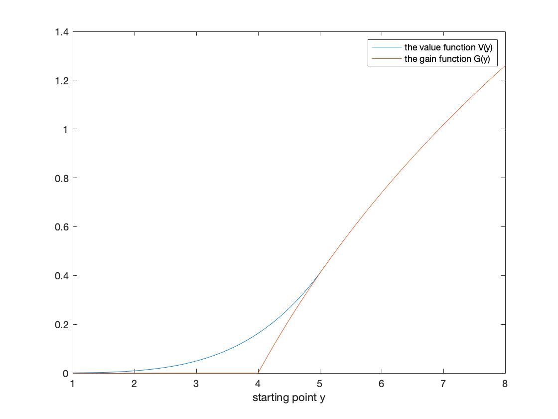
Figure 1: This figure displays the maps $y\mapsto V(y)$ and $y\mapsto G(y)$ with chosen parameters $L=4$, $r=0.02$, $\sigma=0.3$, $\lambda=0.5$ and the optimal stopping point $b=5.0845$.

3 Finite-time Horizon

3.1 Reformulation and Basics

In this section, we consider problem (1.3) in the finite time horizon and by the same arguments as that in Section 2, it can be reformulated as

$$V =\sup_{0\leq\tau\leq{T}}E_{0,x,s}\left(e^{-(r+\lambda)\tau}(S_{\tau}-LX_{\tau})^{+}P(\theta>\tau\,|\,{\cal F}_{\tau})\right).$$ (3.26)

Once again, some general facts of the Azéma supermartingale associated with random time $\theta$ to start the ball rolling. For notational convenience, we set

$$Z(t,y)=\Phi\left(\frac{-\log{y}+\left(r-\frac{\sigma^{2}}{2}\right)(T-t)}{\sigma\sqrt{T-t}}\right)+{y}^{\alpha}\Phi\left(\frac{-\log{y}-\left(r-\frac{\sigma^{2}}{2}\right)(T-t)}{\sigma\sqrt{T-t}}\right),$$

where $\Phi(x)=\frac{1}{\sqrt{2\pi}}\int_{-\infty}^{x}e^{-\frac{z^{2}}{2}}dz$ and $\alpha=\frac{2r}{\sigma^{2}}-1<0$.

Proposition 3.1.

Let $P(\theta>t|\mathcal{F}_{t})$ be the Azéma supermartingale of random time $\theta$. Then

$$P(\theta>t|\mathcal{F}_{t}) =Z(t,Y_{t}),$$ (3.27)

where $Y$ is the process introduced in Corollary 2.3.

Proof.

From the set equality

$$\{\theta>t\}=\left\{\max_{t\leq u\leq T}X_{u}>S_{t}\right\},$$

we deduce that

$$P(\theta>t|\mathcal{F}_{t}) =P\left(\max_{t\leq u\leq T}X_{u}>S_{t}\big{|}\mathcal{F}_{t}\right)=P\left(\frac{\max_{t\leq u\leq T}X_{u}}{X_{t}}>\frac{S_{t}}{X_{t}}\bigg{|}\mathcal{F}_{t}\right)$$

$$=P\left(\log{\frac{S_{t}}{X_{t}}}<\max_{0\leq u\leq T-t}{\left(r-\frac{\sigma^{2}}{2}\right)u+\sigma W_{u}}\right)$$

$$=P\left(\log{Y_{t}}<\max_{0\leq u\leq T-t}{\left(r-\frac{\sigma^{2}}{2}\right)u+\sigma W_{u}}\right),$$ (3.28)

and by applying the general result from [16, Page 759-760] to equation (3.28), the conclusion is immediate. ∎

Remark 3.2.

As the reader may have discovered, we have not yet defined $\theta$ properly if the process $X$ does not exceed level $s$ at all on $[0,T]$, given that $x<s$. However, it should now be clear that in such case, by Proposition 3.1, $P\left(\theta>t|\mathcal{F}_{t}\right)=0$ so that there is nothing to prove and thus the definition shall not concern us. Another more convenient way for this is to simply define the $\sup\{\emptyset\}=0$, see [8, Page 296], after which, the same result follows.

Proposition 3.3.

The function $Z(t,y)$ satisfies the PDE for $(t,x)\in[0,T]\times(1,\infty)$.

$$\frac{\partial Z(t,y)}{\partial t}+(\sigma^{2}-r)y\frac{\partial Z(t,y)}{\partial y}+\frac{1}{2}\sigma^{2}y^{2}\frac{\partial^{2}Z(t,y)}{\partial y^{2}}=0.$$ (3.29)

Proof.

To prove (3.29), we first apply Itô’s formula and obtian

$$dZ(t,Y_{t}) =\left(\frac{\partial Z}{\partial t}+(\sigma^{2}-r)y\frac{\partial Z}{\partial y}+\frac{1}{2}\sigma^{2}y^{2}\frac{\partial^{2}Z}{\partial y^{2}}\right)(t,Y_{t})dt$$

$$\qquad\qquad\,\,\,\,\,\,\,+\frac{\partial Z}{\partial y}(t,Y_{t})dR_{t}-\sigma Y_{t}\ \frac{\partial Z}{\partial y}(t,Y_{t})dW_{t}.$$ (3.30)

Then, recall the Doob-Meyer decomposition of the Azéma supermartingale, that is,

$$Z(t,Y_{t})=Z(0,Y_{0})+M_{t}^{\theta}-A_{t}^{\theta},$$ (3.31)

moreover, the measure $dA_{t}^{\theta}$ is carried by the set $\{t:X_{t}=S_{t}\}$.

The conclusion now follows from the uniqueness of the Doob-Meyer decomposition, upon comparing (3.30) and (3.31), more precisely, we have

$$M_{t}^{\theta}=-\sigma\int_{0}^{t}Y_{u}\ \frac{\partial Z}{\partial y}(u,Y_{u})dW_{u},\qquad A_{t}^{\theta}=-\int_{0}^{t\wedge T}\frac{\partial Z}{\partial y}(u,Y_{u})dR_{u}.$$

∎

The following result is simple yet useful, which we state for easy reference.

Corollary 3.4.

Both maps $t\mapsto Z(t,y)$ and $y\mapsto Z(t,y)$ are decreasing.

Proof.

Immediate from (A.78) and (A.79). ∎

For the sake of brevity, we set the gain function

$$G(t,y)=(y-L)^{+}Z(t,y).$$

We are now in the position to reduce the original problem (3.26) to one-dimension by using the measure $\widetilde{P}$ and generalise it by the strong Markov property of the process $Y$, that is

$$V(t,y) =\sup_{0\leq\tau\leq{T-t}}{E}_{t,x,s}\left(e^{-(r+\lambda)\tau}X_{t+\tau}\left(\frac{S_{t+\tau}}{X_{t+\tau}}-L\right)^{+}P(\theta>t+\tau\,|\,{\cal F}_{t+\tau})\right)$$

$$=\sup_{0\leq\tau\leq{T-t}}\widetilde{E}_{t,y}\left(e^{-\lambda\tau}\left(Y_{t+\tau}-L\right)^{+}Z(t+\tau,Y_{t+\tau})\right)$$

$$=\sup_{0\leq\tau\leq{T-t}}\widetilde{E}_{t,y}\left(e^{-\lambda\tau}G(t+\tau,Y_{t+\tau})\right),$$ (3.32)

where $\tau$ is a stopping time of the diffusion process $Y$ with $Y_{t}=y$ under $\widetilde{P}_{t,y}$ for $(t,y)\in[0,T]\times[1,\infty)$ given and fixed.

3.2 The Free-boundary Problem

In order to formulate and describe the free-boundary problem, it is convenient to introduce the following sets.

Definition 3.5.

The continuation set and the stopping set are defined respectively as

$$\mathcal{C}=\{(t,y)\in[0,T)\times[1,\infty):V(t,y)>G(t,y)\},$$ (3.33)

$$\mathcal{D}=\{(t,y)\in[0,T)\times[1,\infty):V(t,y)=G(t,y)\}\cup\{\{T\}\times[1,\infty)\}.$$ (3.34)

and we define the first entrance time of the stopping set $\mathcal{D}$, denoted as $\tau_{\mathcal{D}}$, as follows

$$\tau_{\mathcal{D}}=\inf\{s\geq 0:Y_{t+s}^{y}\in\mathcal{D}\}\wedge(T-t).$$ (3.35)

Remark 3.6.

In the finite-time case, we have $\tau_{\mathcal{D}}\leq T-t<\infty$ a.s, thus the condition $\widetilde{P}(\tau_{\mathcal{D}}<\infty)=1$ is automatically satisfied for all $y\in[1,\infty)$.

Having defined stopping time $\tau_{\mathcal{D}}$, another natural challenge is to determine the optimality of $\tau_{\mathcal{D}}$. To do so, we begin by showing that the value function $V$ is continuous.

Lemma 3.7.

The value function $V$ is continuous on $[0,T)\times[1,\infty)$.

Proof.

We first show that (i) $t\mapsto V(t,y)$ is continuous on $[0,T)$ for each $y\geq 1$ given and fixed. Take any $t_{1}<t_{2}$ in $[0,T)$, $\epsilon>0$ and let $\tau_{1}^{\epsilon}$ be a stopping time such that $\widetilde{P}_{t_{1},y}\left(\tau_{1}^{\epsilon}<=T-t_{1}\right)=1$ and that

$$\widetilde{E}_{t_{1},y}\left(e^{-\lambda\tau_{1}^{\epsilon}}\left(Y_{t_{1}+\tau_{1}^{\epsilon}}-L\right)^{+}Z\left(t_{1}+\tau_{1}^{\epsilon},Y_{t_{1}+\tau_{1}^{\epsilon}}\right)\right)\geq V(t_{1},y)-\epsilon,$$

and set $\tau_{2}^{\epsilon}=\tau_{1}^{\epsilon}\wedge(T-t_{2})$, we see that

$$\widetilde{E}_{t_{2},y}\left(e^{-\lambda\tau_{2}^{\epsilon}}\left(Y_{t_{2}+\tau_{2}^{\epsilon}}-L\right)^{+}Z\left(t_{2}+\tau_{2}^{\epsilon},Y_{t_{2}+\tau_{2}^{\epsilon}}\right)\right)\leq V(t_{2},y).$$

Noting that $t\mapsto V(t,y)$ is decreasing (see Lemma A.2) and the time-homogeneous property of process $Y$, we then obtain

$$0 \leq V(t_{1},y)-V(t_{2},y)$$ (3.36)

$$\leq\widetilde{E}\left(e^{-\lambda\tau_{1}^{\epsilon}}\left(Y_{t_{1}+\tau_{1}^{\epsilon}}^{y}-L\right)^{+}Z\left(t_{1}+\tau_{1}^{\epsilon},Y_{t_{1}+\tau_{1}^{\epsilon}}^{y}\right)-e^{-\lambda\tau_{2}^{\epsilon}}\left(Y_{t_{2}+\tau_{2}^{\epsilon}}^{y}-L\right)^{+}Z\left(t_{2}+\tau_{2}^{\epsilon},Y_{t_{2}+\tau_{2}^{\epsilon}}^{y}\right)\right)+\epsilon$$

$$\leq\widetilde{E}\left(e^{-\lambda\tau_{2}^{\epsilon}}\left(\left(Y_{t_{1}+\tau_{1}^{\epsilon}}^{y}-L\right)^{+}Z\left(t_{1}+\tau_{1}^{\epsilon},Y_{t_{1}+\tau_{1}^{\epsilon}}^{y}\right)-\left(Y_{t_{2}+\tau_{2}^{\epsilon}}^{y}-L\right)^{+}Z\left(t_{2}+\tau_{2}^{\epsilon},Y_{t_{2}+\tau_{2}^{\epsilon}}^{y}\right)\right)\right)+\epsilon$$

$$\leq\widetilde{E}\left(\left(Y_{t_{1}+\tau_{1}^{\epsilon}}^{y}-L\right)^{+}Z\left(t_{1}+\tau_{1}^{\epsilon},Y_{t_{1}+\tau_{1}^{\epsilon}}^{y}\right)-\left(Y_{t_{2}+\tau_{2}^{\epsilon}}^{y}-L\right)^{+}Z\left(t_{2}+\tau_{2}^{\epsilon},Y_{t_{2}+\tau_{2}^{\epsilon}}^{y}\right)\right)+\epsilon$$

$$\leq\widetilde{E}\left(\left(Y_{t_{1}+\tau_{1}^{\epsilon}}^{y}-Y_{t_{2}+\tau_{2}^{\epsilon}}^{y}\right)^{+}Z\left(t_{1}+\tau_{1}^{\epsilon},Y_{t_{1}+\tau_{1}^{\epsilon}}^{y}\right)\right.$$

$$\qquad\qquad+\left.\left(Y_{t_{2}+\tau_{2}^{\epsilon}}^{y}-L\right)^{+}\left(Z\left(t_{1}+\tau_{1}^{\epsilon},Y_{t_{1}+\tau_{1}^{\epsilon}}^{y}\right)-Z\left(t_{2}+\tau_{2}^{\epsilon},Y_{t_{2}+\tau_{2}^{\epsilon}}^{y}\right)\right)\right)+\epsilon,$$ (3.37)

where the last inequality follows from

$$(x-z)^{+}-(y-z)^{+}\leq(x-y)^{+}\qquad\text{for $x,y,z\in\mathbb{R}$}.$$ (3.38)

Hence, by letting $t_{1}\to t_{2}$ and $\epsilon\to 0$, $\tau_{1}^{\epsilon}\to\tau_{2}^{\epsilon}$, the dominated convergence theorem (see (A.81) for the uniform integrability of $Y$) yields

$$V(t_{1},y)-V(t_{2},y)\to 0$$

which finishes the first part of the proof.

We then show that (ii) $y\mapsto V(t,y)$ is continuous for all $t\in[0,T)$. For this, we note that for all $1\leq y_{1}<y_{2}<\infty$ and $t\in[0,T)$,

$$0\leq\left|V(t,y_{2})-V(t,y_{1})\right|$$

$$\leq\sup_{0\leq\tau\leq T-t}\left|\widetilde{E}\left(\left(\frac{y_{2}\vee S_{\tau}}{X_{\tau}}-L\right)^{+}Z\left(t+\tau,\frac{y_{2}\vee S_{\tau}}{X_{\tau}}\right)-\left(\frac{y_{1}\vee S_{\tau}}{X_{\tau}}-L\right)^{+}Z\left(t+\tau,\frac{y_{1}\vee S_{\tau}}{X_{\tau}}\right)\right)\right|$$

$$\leq\sup_{0\leq\tau\leq T-t}\widetilde{E}\left|\left(\frac{y_{2}\vee S_{\tau}}{X_{\tau}}-L\right)^{+}Z\left(t+\tau,\frac{y_{2}\vee S_{\tau}}{X_{\tau}}\right)-\left(\frac{y_{1}\vee S_{\tau}}{X_{\tau}}-L\right)^{+}Z\left(t+\tau,\frac{y_{1}\vee S_{\tau}}{X_{\tau}}\right)\right|$$

$$\leq\sup_{0\leq\tau\leq T-t}\widetilde{E}\left|\left(\left(\frac{y_{2}\vee S_{\tau}}{X_{\tau}}-L\right)^{+}-\left(\frac{y_{1}\vee S_{\tau}}{X_{\tau}}-L\right)^{+}\right)Z\left(t+\tau,\frac{y_{2}\vee S_{\tau}}{X_{\tau}}\right)\right|$$

$$\qquad\qquad\,\,\,\,\,\,\,+\sup_{0\leq\tau\leq T-t}\widetilde{E}\left|\left(\frac{y_{1}\vee S_{\tau}}{X_{\tau}}-L\right)^{+}\left(Z\left(t+\tau,\frac{y_{2}\vee S_{\tau}}{X_{\tau}}\right)-Z\left(t+\tau,\frac{y_{1}\vee S_{\tau}}{X_{\tau}}\right)\right)\right|$$

$$\leq\sup_{0\leq\tau\leq T-t}\widetilde{E}\left|\left(\frac{\left(y_{2}-S_{\tau}\right)^{+}+S_{\tau}}{X_{\tau}}-\frac{\left(y_{1}-S_{\tau}\right)^{+}+S_{\tau}}{X_{\tau}}\right)Z\left(t+\tau,\frac{y_{2}\vee S_{\tau}}{X_{\tau}}\right)\right|$$

$$\qquad\qquad\,\,\,\,\,\,\,+\sup_{0\leq\tau\leq T-t}\widetilde{E}\left|\left(\frac{y_{1}\vee S_{\tau}}{X_{\tau}}-L\right)^{+}\left(Z\left(t+\tau,\frac{y_{2}\vee S_{\tau}}{X_{\tau}}\right)-Z\left(t+\tau,\frac{y_{1}\vee S_{\tau}}{X_{\tau}}\right)\right)\right|$$

$$\leq(y_{2}-y_{1})\sup_{0\leq\tau\leq T-t}\widetilde{E}\left(\frac{1}{X_{\tau}}\right)$$

$$\qquad\qquad\,\,\,\,\,\,\,+\sup_{0\leq\tau\leq T-t}\widetilde{E}\left|\left(\frac{y_{1}\vee S_{\tau}}{X_{\tau}}-L\right)^{+}\left(Z\left(t+\tau,\frac{y_{2}\vee S_{\tau}}{X_{\tau}}\right)-Z\left(t+\tau,\frac{y_{1}\vee S_{\tau}}{X_{\tau}}\right)\right)\right|$$

$$\leq(y_{2}-y_{1})+\sup_{0\leq\tau\leq T-t}\widetilde{E}\left|\left(\frac{y_{1}\vee S_{\tau}}{X_{\tau}}-L\right)^{+}\left(Z\left(t+\tau,\frac{y_{2}\vee S_{\tau}}{X_{\tau}}\right)-Z\left(t+\tau,\frac{y_{1}\vee S_{\tau}}{X_{\tau}}\right)\right)\right|,$$

$$\leq(y_{2}-y_{1})+\sup_{0\leq\tau\leq T-t}\widetilde{E}\left|Y_{\tau}^{y_{1}}\left(\frac{y_{2}\vee S_{\tau}}{X_{\tau}}-\frac{y_{1}\vee S_{\tau}}{X_{\tau}}\right)Z_{y}\left(t+\tau,\frac{y_{3}\vee S_{\tau}}{X_{\tau}}\right)I\bigg{\{}\frac{y_{1}\vee S_{\tau}}{X_{\tau}}>L\bigg{\}}\right|,$$

$$\leq(y_{2}-y_{1})+C_{1}(y_{2}-y_{1})\sup_{0\leq\tau\leq T-t}\widetilde{E}\left|\frac{Y_{\tau}^{y_{1}}}{X_{\tau}}\right|$$ (3.39)

where the second inequality holds by

$$\left|\sup{f}-\sup{g}\right|\leq\sup{\left|f-g\right|},$$

and the fourth inequality follows via the triangle inequality, the fifth inequality is immediate from (3.38) and the seventh one follows from

$$\frac{1}{X_{t}}=e^{-\left(r+\frac{\sigma^{2}}{2}\right)t-\sigma\widetilde{W}_{t}}\leq e^{-\frac{\sigma^{2}}{2}t-\sigma\widetilde{W}_{t}},$$

where the last term is the martingale under probability measure $\widetilde{P}$; and the ninth inequality is due to the mean value theorem for $y_{3}\in[y_{1},y_{2}]$ so that $\frac{y_{1}\vee S_{\tau}}{X_{\tau}}>L$ implies $\frac{y_{3}\vee S_{\tau}}{X_{\tau}}>L$ a.s., while the last two steps are due to the fact that

$$\frac{y_{2}\vee S_{\tau}}{X_{\tau}}-\frac{y_{1}\vee S_{\tau}}{X_{\tau}}=\frac{(y_{2}-S_{\tau})^{+}+S_{\tau}-(y_{1}-S_{\tau})^{+}-S_{\tau}}{X_{\tau}}\leq\frac{(y_{2}-y_{1})^{+}}{X_{\tau}}$$

and (2.6); in addition, note that function $Z_{y}(t,y)$ is bounded by $C_{1}$ for $y>L$ (see A.80) and the boundedness of the second term in the last inequality can be verified via the same fashion as in (A.81). By letting $y_{1}\to y_{2}$,

$$V(t,y_{2})-V(t,y_{1})\to 0,$$

after which statement (ii) follows. ∎

Lemma 3.8.

The stopping time $\tau_{\mathcal{D}}$ is optimal.

Proof.

By Lemma 3.7 and [11, Corollary 2.9, Page 46], the stopping time defined as

$$\bar{\tau}_{D}=\inf\{s\in[0,T-t):\left(t+s,Y_{t+s}^{y}\right)\in\bar{\mathcal{D}}\}$$

is optimal (with the convention that the infimum of the empty set is infinite.) for the following problem

$$\bar{V}(t,y)=\sup_{\tau\in[0,T-t)}\widetilde{E}_{t,y}\left(e^{-\lambda\tau}G\left(t+\tau,Y_{t+\tau}\right)\right),$$

so that $\bar{V}(t,y)=\widetilde{E}_{t,y}\left(e^{-\lambda\bar{\tau}_{D}}G\left(t+\bar{\tau}_{D},Y_{t+\bar{\tau}_{D}}\right)\right)$, where its corresponding stopping set is defined as $\bar{\mathcal{D}}=\mathcal{D}\setminus\{(T,y):y\in[1,\infty)\}$. Furthermore, observe that

$$V(t,y) =\sup_{\tau\in[0,T-t]}\widetilde{E}_{t,y}\left(e^{-\lambda\tau}G\left(t+\tau,Y_{t+\tau}\right)\right)$$

$$=\sup_{\tau\in[0,T-t]}\widetilde{E}_{t,y}\left(e^{-\lambda\tau}G\left(t+\tau,Y_{t+\tau}\right)I\{\tau<T-t\}+e^{-\lambda(T-t)}G\left(T,Y_{T}\right)I\{\tau=T-t\}\right)$$

$$=\max\bigg{\{}\sup_{\tau\in[0,T-t)}\widetilde{E}_{t,y}\left(e^{-\lambda\tau}G\left(t+\tau,Y_{t+\tau}\right)\right),\widetilde{E}_{t,y}\left(e^{-\lambda(T-t)}G\left(T,Y_{T}\right)\right)\bigg{\}}$$

$$=\max\bigg{\{}\widetilde{E}_{t,y}\left(e^{-\lambda\bar{\tau}_{D}}G\left(t+\bar{\tau}_{D},Y_{t+\bar{\tau}_{D}}\right)\right),\widetilde{E}_{t,y}\left(e^{-\lambda(T-t)}G\left(T,Y_{T}\right)\right)\bigg{\}},$$

such that,

$$V(t,y)=\begin{cases}&\widetilde{E}_{t,y}\left(e^{-\lambda\bar{\tau}_{D}}G\left(t+\bar{\tau}_{D},Y_{t+\bar{\tau}_{D}}\right)\right),\,\,\bar{\tau}_{D}<T-t,\\ &\widetilde{E}_{t,y}\left(e^{-\lambda(T-t)}G\left(T,Y_{T}\right)\right),\qquad\,\,\,\bar{\tau}_{D}>T-t,\end{cases}$$

which implies that $\tau_{D}=\bar{\tau}_{D}\wedge(T-t)$, and the desired claim follows. ∎

It will be shown in the next section that the continuation region and the stopping region could also be defined as

$$\mathcal{C}=\{(t,y)\in[0,T)\times[1,\infty):y<b(t)\},$$ (3.40)

$$\mathcal{D}=\{(t,y)\in[0,T)\times[1,\infty):y\geq b(t)\}\cup\{(T,y):y\geq b(T)\},$$ (3.41)

where $b:[0,T]\mapsto\mathbb{R}$ is the unknown optimal stopping boundary, it then follows that $\tau_{\mathcal{D}}$ can be rewritten as

$$\tau_{\mathcal{D}}=\inf\{0\leq s\leq T-t:Y_{t+s}^{y}\geq b(t+s)\}\wedge(T-t).$$

We are now ready to formulate the following free-boundary problem.

After establishing the optimality of $\tau_{\mathcal{D}}$, [11, Theorem 2.4, Page 37] suggest that the unknown value function $V$ from (3.32), together with the unknown boundary $b$, solve

$$V_{t}+\mathbb{L}_{Y}V=\lambda V\qquad\text{in}\,\,\mathcal{C},$$ (3.42)

$$V(t,y)=G(t,y)\qquad\text{for $y=b(t)$ or $t=T$,}$$ (3.43)

$$V_{y}(t,y)=G_{y}(t,y)\,\,\,\,\,\,\,\,\text{for $y=b(t)$}\,\,\textit{(smooth fit)},$$ (3.44)

$$V_{y}(t,1+)=0\qquad\textit{(normal reflection)},$$ (3.45)

$$V(t,y)>G(t,y)\qquad\text{in}\,\,\mathcal{C},$$ (3.46)

$$V(t,y)=G(t,y)\qquad\text{in}\,\,\mathcal{D}.$$ (3.47)

Proofs of conditions (3.44)-(3.45) will be given in section 3.4.

3.3 The Continuation and Stopping Sets

We first need to make some preparations in order to prove (3.40) and (3.41).

Since the gain function $G(t,y)$ is a continuous function whose derivative in $y=L$ is not continuous, we apply the local time-space formula on $e^{-\lambda s}G(t+s,Y_{t+s})$ and obtain

$$e^{-\lambda s}G(t+s,Y_{t+s}) =G(t,y)+\int_{0}^{s}e^{-\lambda u}H(t+u,Y_{t+u})I\{Y_{t+u}>L\}du$$

$$+\int_{0}^{s}e^{-\lambda u}G_{y}(t+u,Y_{t+u})I\{Y_{t+u}=1\}dR_{t+u}+M_{s}$$

$$+\frac{1}{2}\int_{0}^{s}e^{-\lambda u}\left(G_{y}(t+u,L+)-G_{y}(t+u,L-)\right)dl_{u}^{L}(Y),$$ (3.48)

where we set

$$H(t,y) =\left(-\lambda G+\frac{\partial G}{\partial t}-ry\frac{\partial G}{\partial y}+\frac{1}{2}\sigma^{2}y^{2}\frac{\partial^{2}G}{\partial y^{2}}\right)(t,y),$$ (3.49)

and $M_{s}=-\int_{0}^{s}\sigma Y_{t+s}G_{y}(t+s,Y_{t+s})I\{Y_{t+s}\neq L\}d\widetilde{W}_{s}$ is a martingale.

To simplify (3.49), we see that

$$\frac{\partial G}{\partial t}(t,y)=(y-L)\frac{\partial Z(t,y)}{\partial t},$$

$$\frac{\partial G}{\partial y}(t,y)=Z(t,y)+(y-L)\frac{\partial Z(t,y)}{\partial y},$$

$$\frac{\partial^{2}G}{\partial y^{2}}(t,y)=2\frac{\partial Z(t,y)}{\partial y}+(y-L)\frac{\partial^{2}Z(t,y)}{\partial y^{2}},$$

for all $y>L$.

By combining the above computation and using the fact that $Z(t,y)$ satisfying (3.29), we therefore have (3.49) rewritten as follows

$$H(t,y)=\left(-\lambda(y-L)Z-ryZ+\sigma^{2}Ly\frac{\partial Z}{\partial y}\right)(t,y).$$

Then, by taking the expectation under $\widetilde{P}_{t,y}$ and applying the optional sampling theorem to get rid of the martingale part, we find that

$$\widetilde{E}_{t,y}\left(e^{-\lambda s}G(t+s,Y_{t+s})\right) =G(t,y)+\widetilde{E}_{t,y}\int_{0}^{s}e^{-\lambda u}H(t+u,Y_{t+u})I\{Y_{t+u}>L\}du$$

$$+\widetilde{E}_{t,y}\int_{0}^{s}e^{-\lambda u}G_{y}(t+u,1+)I\{Y_{t+u}\neq L\}dR_{t+u}$$

$$+\frac{1}{2}\widetilde{E}_{t,y}\int_{0}^{s}e^{-\lambda u}\left(G_{y}(t+u,L+)-G_{y}(t+u,L-)\right)dl_{u}^{L}(Y).$$ (3.50)

We first investigate the map $t\mapsto H(t,y)$ by a direct differentiation in $t$, which yields

$$\frac{\partial H}{\partial t}(t,y) =-(ry+\lambda y-\lambda L)\frac{\partial Z}{\partial t}+\sigma^{2}Ly\frac{\partial^{2}Z}{\partial y\partial t}$$

$$=\frac{y^{\alpha}e^{-\frac{d_{2}^{2}}{2}}}{\sqrt{8\pi}(T-t)^{\frac{3}{2}}}\left(\frac{-2(ry+\lambda y-\lambda L)\log{y}}{\sigma}+2\sigma^{2}L-\frac{2(\log{y})^{2}L}{T-t}+(2r-\sigma^{2})L\log{y}\right)$$

$$<\frac{y^{\alpha}e^{-\frac{d_{2}^{2}}{2}}L}{\sqrt{8\pi}(T-t)^{\frac{3}{2}}}\left(-\frac{2r\log{L}}{\sigma}+2\sigma^{2}-\frac{2(\log{L})^{2}}{T}+(2r-\sigma^{2})\log{L}\right),$$ (3.51)

from which one sees that there exists a wide range of parameters for $t\mapsto H(t,y)$ to be decreasing.

Remark 3.9.

The map $t\mapsto H(t,y)$ being decreasing is rather crucial for showing the monotonicity of $b$, the continuity of $b$ and the smooth-fit condition.

For the purpose of proving the properties mentioned in Remark 3.9, from now on, we assume:

Assumption 3.10.

Parameters $r$ and $\sigma$ can be chosen so that the map $t\mapsto H(t,x)$ is decreasing.

Lemma 3.11.

The continuation set $\mathcal{C}$ is left-connected and non-increasing with respect to time $t$.

Proof.

We shall show that for fixed $0\leq t_{1}<t_{2}<T$ and $y\in(L,\infty)$, $(t_{2},y)\in\mathcal{C}$ implies $(t_{1},y)\in\mathcal{C}$.

We begin by recalling that

$$G_{y}(t,y)=\begin{cases}0,&\text{for $y\leq L$},\\ Z(t,y)+(y-L)\frac{\partial Z(t,y)}{\partial y},&\text{for $y>L$},\end{cases}$$

and for $L>1$, it follows that

$$G_{y}(t,1+)=0,$$ (3.52)

$$G_{y}(t,L+)=Z(t,L+),$$ (3.53)

$$G_{y}(t,L-)=0.$$ (3.54)

Let $\tau$ be the optimal stopping time for $V(t_{2},y)$ so that by (3.50) and (3.52)-(3.54),

$$V(t_{1},y)-V(t_{2},y)\geq\widetilde{E}\left(e^{-\lambda\tau}G(t_{1}+\tau,Y_{t_{1}+\tau}^{y})\right)-\widetilde{E}\left(e^{-\lambda\tau}G(t_{2}+\tau,Y_{t_{2}+\tau}^{y})\right)$$

$$\qquad=\widetilde{E}\left(e^{-\lambda\tau}G(t_{1}+\tau,Y_{\tau}^{y})\right)-\widetilde{E}\left(e^{-\lambda\tau}G(t_{2}+\tau,Y_{\tau}^{y})\right)$$

$$\qquad=G(t_{1},y)-G(t_{2},y)+\widetilde{E}\left(\int_{0}^{\tau}e^{-\lambda u}\left(H(t_{1}+u,Y_{u}^{y})-H(t_{2}+u,Y_{u}^{y})\right)I\{Y_{u}^{y}>L\}du\right)$$

$$\qquad\qquad+\frac{1}{2}\widetilde{E}\left(\int_{0}^{\tau}e^{-\lambda u}\left(G_{y}(t_{1}+u,L+)-G_{y}(t_{2}+u,L+)\right)dl_{u}^{L}(Y)\right)$$

$$\qquad\geq G(t_{1},y)-G(t_{2},y),$$

where the first equality holds as $Y_{t_{1}+\tau}^{y}$, $Y_{t_{2}+\tau}^{y}$ and $Y_{\tau}^{y}$ are identically distributed and the last inequality holds by the fact that both $t\mapsto H(t,y)$ and $t\mapsto G_{y}(t,L+)$ are decreasing on $[0,T]$. Hence, we reach the following conclusion

$$V(t_{1},y)-G(t_{1},y)\geq V(t_{2},y)-G(t_{2},y),$$ (3.55)

indicating that if a point $(t_{2},y)\in\mathcal{C}$, then we have $V(t_{1},y)-G(t_{1},y)\geq V(t_{2},y)-G(t_{2},y)>0$, which implies that $(t_{1}.y)\in\mathcal{C}$, proving the initial claim. ∎

From (3.55), the following statement does not come to us as a surprise, that is the map $t\mapsto V(t,y)-G(t,y)$ is decreasing on $[0,T]$.

Lemma 3.12.

The stopping set $\mathcal{D}$ is right-connected and up-connected.

Proof.

The right-connectedness of the stopping set $\mathcal{D}$ is another direct consequence of (3.55), since

$$0=V(t_{1},y)-G(t_{1},y)\geq V(t_{2},y)-G(t_{2},y)\geq 0,$$

that is, $(t_{1},y)\in\mathcal{D}$ implies $(t_{2},y)\in\mathcal{D}$.

To justify its up-connectedness, we first take $t>0$ and $y_{2}>y_{1}>L$ such that $(t,y_{1})\in\mathcal{D}$. Then, by the right-connectedness of the exercise region, we have $(t+s,y_{1})\in\mathcal{D}$ for any $s\in(0,T-t)$. If we now run the process $(t+s,Y_{t+s}^{y_{2}})$ from $(t,y_{2})$, we cannot hit the level $L$ to compensate the negative integrant $H$ in (3.50) before exercise as $y_{2}>y_{1}$, which means that the local time term in (3.50) is 0 and the integrand $H$ is negative. Therefore, it’s optimal to exercise at $(t,y_{2})$ and we have established the up-connectedness of the exercise region $\mathcal{D}$. ∎

Lemma 3.13.

The map $t\mapsto b(t)$ is decreasing on $[0,T]$.

Proof.

Combine Lemma 3.11 and Lemma 3.12. ∎

Proposition 3.14.

All points $y<L$ for $0\leq t<T$ belongs to the continuation set $\mathcal{C}$.

Proof.

The proof follows, in fact, from the verbal statement, by exercising below $L$, the option holder receive a null payoff, whereas waiting would have a positive probability of collecting a strictly positive payoff in the future.

A more detailed yet simple proof of this is that, from (3.50), we know that for $Y_{t}^{y}<L$, all integral terms on the right-hand side are nonnegative. ∎

We also recall the solution to the infinite time horizon optimal stopping problem, where the stopping time $\tau_{b}=\inf\{t\geq 0:Y_{t}>b_{*}\}$ is optimal and $b_{*}>L$ is proved to be true, we therefore conclude that all points $(t,y)$ with $y>b_{*}$ for $0<t\leq T$ belong to the stopping set $\mathcal{D}$ and that as $b_{*}$ is finite, so is $b$.

By taking advantage of our findings so far, we can draw the conclusion that the continuation set $\mathcal{C}$ and the stopping set $\mathcal{D}$ indeed equal (3.40) and (3.41) respectively.

We close this section by constructing the continuity of the optimal stopping boundary $b$.

Proposition 3.15.

The optimal stopping boundary $b$ is continuous on $[0,T]$ and $b(T-)=L$.

Proof.

We first show that (i) $b$ is right-continuous. Let us fix $t\in[0,T)$ and take a sequence $t_{n}\downarrow t$ as $n\to\infty$. Since $b$ is decreasing on $[0,T]$, the right-limit $b(t+)$ exists. Remember that $\mathcal{D}$ is closed so that its limit point $\lim\limits_{n\to\infty}(t_{n},b(t_{n}))\to(t,b(t+))$ is contained in $\mathcal{D}$ , it then follows, together with (3.41), that $b(t+)\geq b(t)$. However, the fact that $b$ is decreasing suggests that $b(t)\geq b(t+)$ and therefore, $b$ is right-continuous as claimed.

We then show that (ii) $b$ is left-continuous. Assume that, for contradiction, there exists $t\in(0,T)$ such that $b(t-)>b(t)$. Then, fix a point $y_{*}\in(b(t),b(t-))$.

By (3.43) and (3.44), we have

$$V(s,y_{*})-G(s,y_{*}) =\int_{y_{*}}^{b(s)}\int_{x}^{b(s)}\left(V_{yy}-G_{yy}\right)(s,z)dzdx,$$ (3.56)

for each $s\in(t-\delta,t)$ where $\delta>0$ and $t-\delta>0$. Knowing that the value function satisfies

$$V_{t}+\mathbb{L}_{Y}V=\lambda V,\qquad\text{in $\mathcal{C}$},$$

and that

$$H(t,y)=\left(-\lambda G+G_{t}+\mathbb{L}_{Y}G\right)(t,y),$$

we have

$$\frac{\sigma^{2}y^{2}}{2}\left(V_{yy}-G_{yy}\right)(t,y) =\left(\lambda(V-G)-(V_{t}-G_{t})+ry(V_{y}-G_{y})-H\right)(t,y).$$

Now recall that $t\mapsto V(t,y)-G(t,y)$ is decreasing and hence

$$\frac{\sigma^{2}y^{2}}{2}\left(V_{yy}-G_{yy}\right)(t,y)\geq\left(ry(V_{y}-G_{y})-H\right)(t,y),$$ (3.57)

in $\mathcal{C}\cup\{(t,y)\in[0,T]\times[1,\infty):y=b(t)\}$.

Using (3.56) and (3.57), we find that

$$V(s,y_{*})-G(s,y_{*}) \geq\int_{y_{*}}^{b(s)}\int_{x}^{b(s)}\left(\frac{2r}{\sigma^{2}z}\left(V_{z}-G_{z}\right)-\frac{2}{\sigma^{2}z^{2}}H\right)(s,z)dzdx,$$

and since $H$ is strictly negative in $\{(s,y)\in[t-\delta,t]\times[y_{*},b(t-\delta)]\}$ (as $y_{*}>b(t)\geq L$), we set

$$m=\inf\bigg{\{}-\frac{2}{\sigma^{2}y^{2}}H(s,y):(s,y)\in[t-\delta,t]\times[y_{*},b(t-\delta)]\bigg{\}}>0,$$

so that

$$V(s,y_{*})-G(s,y_{*}) \geq\frac{2r}{\sigma^{2}}\int_{y_{*}}^{b(s)}\int_{x}^{b(s)}\frac{1}{z}\left(V_{z}-G_{z}\right)(s,z)dzdx+m\int_{y_{*}}^{b(s)}(b(s)-x)dx.$$

Via an integration by parts, we have

$$\int_{y_{*}}^{b(s)}\int_{x}^{b(s)}\frac{1}{z}d\left(V-G\right)(s,z)dx$$

$$\qquad\qquad=\int_{y_{*}}^{b(s)}\left(\frac{1}{z}\left(V-G\right)(s,z)\big{|}_{x}^{b(s)}+\int_{x}^{b(s)}\frac{1}{z^{2}}\left(V-G\right)(s,z)dz\right)dx$$

$$\qquad\qquad=\int_{y_{*}}^{b(s)}-\frac{1}{x}\left(V-G\right)(s,x)dx+\int_{y_{*}}^{b(s)}\int_{x}^{b(s)}\frac{1}{z^{2}}\left(V-G\right)(s,z)dzdx,$$

where the second equality follows from (3.43).

From Lemma 3.7 and the fact that the gain function is continuous on $(1,\infty)\times[0,T]$, we know that

$$V(t,y)=V(t-,y),$$

$$G(t,y)=G(t-,y),$$

and from (3.47), it follows that

$$V(t,y)=G(t,y)\,\,\text{for all $y\in[y_{*},b(t-))$}.$$

Then, we observe that

$$\big{|}V-G\big{|}(s,y) \leq V(s,y)\leq\sup_{0\leq\tau\leq{T-s}}\widetilde{E}_{s,y}\left(Y_{s+\tau}^{y}\right)\leq ye^{\left(r+\frac{\sigma^{2}}{2}\right)T}\widetilde{E}\left(e^{2\sigma\sqrt{T}X}\right)<\infty,$$

where the third inequality holds via (A.81). Finally, let $s\uparrow t$ and an application of the dominated convergence theorem shows

$$V(t,y_{*})-G(t,y_{*}) \geq\frac{2r}{\sigma^{2}}\left(\int_{y_{*}}^{b(t-)}-\frac{1}{x}\left(V-G\right)(t,x)dx+\int_{y_{*}}^{b(t-)}\int_{x}^{b(t-)}\frac{1}{z^{2}}\left(V-G\right)(t,z)dzdx\right)$$

$$\,\,\,+m\int_{y_{*}}^{b(t-)}(b(t-)-x)dx$$

$$=m\int_{y_{*}}^{b(t-)}(b(t-)-x)dx=\frac{m}{2}\left(b(t-)-y_{*}\right)^{2}>0,$$

where the first equality is due to the fact that $\{t\}\times[y_{*},b(t-)]\subset\mathcal{D}$, which is a contradiction, as $(t,y_{*})$ belongs to the stopping set $\mathcal{D}$, indicating that such point cannot exist. Therefore, by combining statements (i) and (ii), we have established the continuity of $b$ on $[0,T]$.

(iii) It remains to take care of the final piece of the claim, that is, $b(T-)=L$.

According to Proposition 3.14, we must have $b(T-)\geq L$. Assume that, $b(T-)>L$ such that a point $y_{*}$ exists on $(L,b(T-))$ and let $s$ be an arbitrarily fixed point in the interval $(T-\delta,T)$ with $0<\delta<T$. Rerunning the proof of (ii) with the above modifications, upon letting $s\uparrow T$, we thus have arrived at the contradiction, that is

$$V(T,y_{*})-G(T,y_{*})>0,$$

but the definition of the stopping set $\mathcal{D}$ tells us that $V(T,y_{*})=G(T,y_{*})$ , which may allow us to conclude that $b(T-)=L$. ∎

3.4 The Optimal Stopping Rule

Before we turn to presenting the main result, let us first complete the promise given in section 3.2, namely, to verify conditions (3.44)-(3.45) for the value function.

Lemma 3.16.

(Smooth-fit Condition) The value function $V(t,y)$ is differentiable at the optimal stopping boundary $b$ and

$$\frac{\partial}{\partial y}V(t,y)=\frac{\partial}{\partial y}G(t,y),$$

whenever $V(t,y)=G(t,y)$ for $y=b(t)$.

Proof.

Let $t\in[0,T)$ be given and fixed and set $y=b(t)$. Knowing that $b(t)>L$, let $\epsilon>0$ so that $y-\epsilon>L$. Since

$$V(t,y)=G(t,y),$$

$$V(t,y-\epsilon)>G(t,y-\epsilon),$$

we have

$$\frac{V(t,y)-V(t,y-\epsilon)}{\epsilon}\leq\frac{G(t,y)-G(t,y-\epsilon)}{\epsilon},$$ (3.58)

and taking the limit as $\epsilon\to 0$ shows that

$$\lim_{\epsilon\to 0}\frac{V(t,y)-V(t,y-\epsilon)}{\epsilon} \leq\lim_{\epsilon\to 0}\frac{G(t,y)-G(t,y-\epsilon)}{\epsilon}=\frac{\partial}{\partial y}G(t,y).$$

To prove the reverse inequality, let $\tau_{\epsilon}$ be the optimal stopping time for $V(t,y-\epsilon)$, so that

$$\frac{V(t,y)-V(t,y-\epsilon)}{\epsilon}\geq\frac{1}{\epsilon}\widetilde{E}\left(e^{-\lambda\tau_{\epsilon}}\left(G\left(t+\tau_{\epsilon},Y_{t+\tau_{\epsilon}}^{y}\right)-G\left(t+\tau_{\epsilon},Y_{t+\tau_{\epsilon}}^{y-\epsilon}\right)\right)\right)$$

$$\,\,\,=\frac{1}{\epsilon}\widetilde{E}\left(e^{-\lambda\tau_{\epsilon}}\left(\left(Y_{t+\tau_{\epsilon}}^{y}-L\right)^{+}-\left(Y_{t+\tau_{\epsilon}}^{y-\epsilon}-L\right)^{+}\right)Z\left(t+\tau_{\epsilon},Y_{t+\tau_{\epsilon}}^{y}\right)\right)$$

$$\,\,\,\qquad+\frac{1}{\epsilon}\widetilde{E}\left(e^{-\lambda\tau_{\epsilon}}\left(Z\left(t+\tau_{\epsilon},Y_{t+\tau_{\epsilon}}^{y}\right)-Z\left(t+\tau_{\epsilon},Y_{t+\tau_{\epsilon}}^{y-\epsilon}\right)\right)\left(Y_{t+\tau_{\epsilon}}^{y-\epsilon}-L\right)^{+}\right)$$

$$\,\,\,\geq\frac{1}{\epsilon}\widetilde{E}\left(e^{-\lambda\tau_{\epsilon}}I\{Y_{t+\tau_{\epsilon}}^{y-\epsilon}\geq L\}\left(Y_{t+\tau_{\epsilon}}^{y}-Y_{t+\tau_{\epsilon}}^{y-\epsilon}\right)Z\left(t+\tau_{\epsilon},Y_{t+\tau_{\epsilon}}^{y}\right)\right)$$

$$\,\,\,\qquad+\frac{1}{\epsilon}\widetilde{E}\left(e^{-\lambda\tau_{\epsilon}}\left(Z\left(t+\tau_{\epsilon},Y_{t+\tau_{\epsilon}}^{y}\right)-Z\left(t+\tau_{\epsilon},Y_{t+\tau_{\epsilon}}^{y-\epsilon}\right)\right)\left(Y_{t+\tau_{\epsilon}}^{y-\epsilon}-L\right)^{+}\right)$$

$$\,\,\,\geq\frac{1}{\epsilon}\widetilde{E}\left(e^{-\lambda\tau_{\epsilon}}I\{Y_{t+\tau_{\epsilon}}^{y-\epsilon}\geq L\}I\{y-\epsilon\geq S_{\tau_{\epsilon}}\}\frac{\epsilon}{X_{\tau_{\epsilon}}}Z\left(t+\tau_{\epsilon},Y_{t+\tau_{\epsilon}}^{y}\right)\right)$$

$$\,\,\,\qquad+\frac{1}{\epsilon}\widetilde{E}\left(e^{-\lambda\tau_{\epsilon}}\left(Z\left(t+\tau_{\epsilon},Y_{t+\tau_{\epsilon}}^{y}\right)-Z\left(t+\tau_{\epsilon},Y_{t+\tau_{\epsilon}}^{y-\epsilon}\right)\right)\left(Y_{t+\tau_{\epsilon}}^{y-\epsilon}-L\right)^{+}\right)$$

$$\,\,\,=\widetilde{E}\left(e^{-\lambda\tau_{\epsilon}}I\{Y_{t+\tau_{\epsilon}}^{y-\epsilon}\geq L\}I\{y-\epsilon\geq S_{\tau_{\epsilon}}\}\frac{1}{X_{\tau_{\epsilon}}}Z\left(t+\tau_{\epsilon},Y_{t+\tau_{\epsilon}}^{y}\right)\right)$$

$$\,\,\,\qquad+\widetilde{E}\left(e^{-\lambda\tau_{\epsilon}}\frac{Z_{y}\left(t+\tau_{\epsilon},Y_{t+\tau_{\epsilon}}^{x}\right)}{X_{\tau_{\epsilon}}}\left(Y_{t+\tau_{\epsilon}}^{y-\epsilon}-L\right)I\{Y_{t+\tau_{\epsilon}}^{y-\epsilon}\geq L\}I\{y-\epsilon\geq S_{\tau_{\epsilon}}\}\right),$$

where the second inequality holds via the facts that $Y_{t+\tau_{\epsilon}}^{y}\geq Y_{t+\tau_{\epsilon}}^{y-\epsilon}$ ($\geq L$ because of the definition of the optimal stopping time) and that

$$\left(Y_{t+\tau_{\epsilon}}^{y}-L\right)^{+}-\left(Y_{t+\tau_{\epsilon}}^{y-\epsilon}-L\right)^{+} =I\{Y_{t+\tau_{\epsilon}}^{y-\epsilon}\geq L\}\left(Y_{t+\tau_{\epsilon}}^{y}-Y_{t+\tau_{\epsilon}}^{y-\epsilon}\right)+\left(Y_{t+\tau_{\epsilon}}^{y}-L\right)^{+}$$

$$\geq I\{Y_{t+\tau_{\epsilon}}^{y-\epsilon}\geq L\}\left(Y_{t+\tau_{\epsilon}}^{y}-Y_{t+\tau_{\epsilon}}^{y-\epsilon}\right),$$

and the third inequality follows from

$$Y_{t+\tau_{\epsilon}}^{y}-Y_{t+\tau_{\epsilon}}^{y-\epsilon} =\frac{(y-S_{\tau_{\epsilon}})^{+}+S_{\tau_{\epsilon}}-(y-\epsilon-S_{\tau_{\epsilon}})^{+}-S_{\tau_{\epsilon}}}{X_{\tau_{\epsilon}}}$$

$$=\frac{I\{y-\epsilon\geq S_{\tau_{\epsilon}}\}\epsilon+\left(y-S_{\tau_{\epsilon}}\right)^{+}}{X_{\tau_{\epsilon}}}\geq\frac{I\{y-\epsilon\geq S_{\tau_{\epsilon}}\}\epsilon}{X_{\tau_{\epsilon}}},$$

and by mean value theory for $x\in[y-\epsilon,y]$, the last equality follows. Note that $I\{Y_{t+\tau_{\epsilon}}^{y-\epsilon}\geq L\}=1$ implies $I\{Y_{t+\tau_{\epsilon}}^{x}\geq L\}=1$ so that $Z_{y}\left(t+\tau_{\epsilon},Y_{t+\tau_{\epsilon}}^{x}\right)$ is bounded by $C_{1}$.

Finally, let $\epsilon\to 0$ so that $\tau_{\epsilon}\to 0$ a.s (see Lemma A.1) and the dominated convergence theorem once again yields $S_{\tau_{\epsilon}}\to 1$, $X_{\tau_{\epsilon}}\to 1$, $Y_{t+\tau_{\epsilon}}^{x}\to y$, $Y_{t+\tau_{\epsilon}}^{y-\epsilon}\to y$, $Y_{t+\tau_{\epsilon}}^{y}\to y$. Then, recalling that $y=b(t)\geq L>1$, we obtain

$$\lim_{\epsilon\to 0}\frac{V(t,y)-V(t,y-\epsilon)}{\epsilon} \geq Z(t,y)+(y-L)\frac{\partial}{\partial y}Z(t,y)=\frac{\partial}{\partial y}G(t,y),$$ (3.59)

which, joining with (3.58), proves the claim. ∎

Lemma 3.17.

The normal reflection condition holds, that is

$$\frac{\partial}{\partial y}V(t,1+)=0.$$

Proof.

We begin by noticing that from (3.32) and the construction of the process $Y$

$$V(t,y) =\sup_{0\leq\tau\leq{T-t}}\widetilde{E}\left(e^{-\lambda\tau}G\left(t+\tau,\frac{(y-S_{\tau})^{+}+S_{\tau}}{X_{\tau}}\right)\right),$$ (3.60)

and that, in fact, there exists $y_{*}\in(1,L]$ such that the map $y\mapsto G\left(t,y\right)$ is increasing on $[1,y_{*}]$ in the sense that $\frac{\partial}{\partial y}G(t,y)=\left(Z+(y-L)\frac{\partial}{\partial y}Z\right)(t,y)>0$.

It then follows, from the view of (3.60), that $y\mapsto V(t,y)$ is increasing on $[1,y_{*}]$, meaning that $V_{y}(t,1+)\geq 0$ for all $t\in[0,T)$, and moreover, since the value function $V$ is $C^{1,2}$ on the continuation set, we have $t\mapsto V_{y}(t,1+)$ is continuous on $[0,T)$.

Assume that, for contradiction, there exists $t\in[0,T)$ so that $V_{y}(t,1+)>0$. Let $\tau_{D}$ be the optimal stopping time for $V(t,1+)$ and let $\hat{\tau}_{D}=\tau_{D}\wedge s$ for $s\in[0,T-t]$. Then, we apply Itô’s formula and the optional sampling theorem to obtain

$$\widetilde{E}_{t,1}\left(e^{-\lambda\hat{\tau}_{D}}V\left(t+\hat{\tau}_{D},Y_{t+\hat{\tau}_{D}}\right)\right)=V(t,1)+\widetilde{E}_{t,1}\left(\int_{0}^{\hat{\tau}_{D}}e^{-\lambda u}V_{y}(t+u,Y_{t+u})dR_{t+u}\right).$$

Now in order to complete the proof, we need to further establish the martingale property of

$$\bigg{\{}e^{-\lambda\hat{\tau}_{D}}V\left(t+\hat{\tau}_{D},Y_{t+\hat{\tau}_{D}}^{1}\right),\mathcal{F}_{t+\hat{\tau}_{D}}\bigg{\}}_{0\leq\hat{\tau}_{D}\leq T-t}.$$ (3.61)

Let us check the martingale property claimed in (3.61) for all $u\leq\hat{\tau}_{D}$:

$$\widetilde{E}\left(e^{-\lambda\hat{\tau}_{D}}V\left(t+\hat{\tau}_{D},Y_{t+\hat{\tau}_{D}}^{1}\right)\big{|}\mathcal{F}_{t+u}\right)$$

$$\qquad=\widetilde{E}\left(e^{-\lambda\hat{\tau}_{D}}\widetilde{E}_{t+\hat{\tau}_{D},Y_{t+\hat{\tau}_{D}}^{1}}\left(e^{-\lambda(\tau_{D}-\hat{\tau}_{D})}G\left(t+\tau_{D},Y_{t+\tau_{D}}\right)\right)\big{|}\mathcal{F}_{t+u}\right)$$

$$\qquad=\widetilde{E}\left(e^{-\lambda\hat{\tau}_{D}}\widetilde{E}\left(e^{-\lambda(\tau_{D}-\hat{\tau}_{D})}G\left(t+\tau_{D},Y_{t+\tau_{D}}\right)\big{|}\mathcal{F}_{t+\hat{\tau}_{D}}\right)\big{|}\mathcal{F}_{t+u}\right)$$

$$\qquad=\widetilde{E}\left(\widetilde{E}\left(e^{-\lambda\tau_{D}}G\left(t+\tau_{D},Y_{t+\tau_{D}}\right)\big{|}\mathcal{F}_{t+\hat{\tau}_{D}}\right)\big{|}\mathcal{F}_{t+u}\right)$$

$$\qquad=\widetilde{E}\left(e^{-\lambda\tau_{D}}G\left(t+\tau_{D},Y_{t+\tau_{D}}\right)\big{|}\mathcal{F}_{t+u}\right)$$

$$\qquad=e^{-ru}\widetilde{E}_{t+u,Y_{t+u}^{1}}\left(e^{-r(\tau_{D}-u)}G\left(t+\tau_{D},Y_{t+\tau_{D}}\right)\right)=e^{-ru}V\left(t+u,Y_{t+u}^{1}\right),$$

where the first equality follows from the definitions of $\tau_{\mathcal{D}}$ and the value function $V$, the second and the fifth equalities are immediate from the strong Markov property of the process $Y$ whereas the fourth equality holds by smoothing lemma as $\mathcal{F}_{t+u}\subseteq\mathcal{F}_{t+\hat{\tau}_{D}}$, and thereby, proving the martingale property.

With the aid of the above observation, we then obtain

$$\widetilde{E}_{t,1}\left(e^{-\lambda\hat{\tau}_{D}}V\left(t+\hat{\tau}_{D},Y_{t+\hat{\tau}_{D}}\right)\right)=V(t,1),$$

which implies that

$$\widetilde{E}_{t,1}\left(\int_{0}^{\hat{\tau}_{D}}e^{-\lambda u}V_{y}(t+u,Y_{t+u})dR_{t+u}\right)=0.$$

In particular, $V_{y}(t+u,Y_{t+u})dR_{t+u}=V_{y}(t+u,1+)dR_{t+u}$, which, together with the assumption that $V_{y}(t+u,1+)>0$ for all $u\in[0,\hat{\tau}_{D}]$, tells us that

$$\widetilde{E}_{t,1}\left(\int_{0}^{\hat{\tau}_{D}}dR_{t+u}\right)=0.$$ (3.62)

By the solution of (2.7), equation (3.62) and the optional sampling theorem, we see that

$$\widetilde{E}_{t,1}\left(Y_{t+\hat{\tau}_{D}}\right)-1+r\widetilde{E}_{t,1}\int_{0}^{\hat{\tau}_{D}}Y_{t+u}du=0.$$ (3.63)

As $Y_{t+u}>1$ for all $u\in[0,T-t]$, (3.63) implies that $\widetilde{P}_{t,1}(\hat{\tau}_{D}=0)=1$, which is not possible in the sense that the optimal stopping boundary $b>1$ and $\hat{\tau}_{D}>0$, proving the desired assertion. ∎

With a bit more effort, we can verify the following result to apply the local time-space formula freely later.

Corollary 3.18.

Let the function $F(t,y)=e^{-\lambda t}V(t,y)$. Then

$$\text{$F(t,y)$ is $C^{1,2}$ on $\mathcal{C}\cup\mathcal{\bar{D}}$},$$ (3.64)

$$\text{$F_{t}+\mathbb{L}_{Y}F$ is locally bounded $\mathcal{C}\cup\mathcal{\bar{D}}$},$$ (3.65)

$$\text{$t\mapsto F_{y}(t,b(t)\pm)$ is continuous},$$ (3.66)

$$\text{$F_{yy}=F_{1}+F_{2}$ on $\mathcal{C}\cup\mathcal{\bar{D}}$},$$

$$\text{where $F_{1}$ is non-negative and $F_{2}$ is continuous on ${\mathcal{C}}$ and $\mathcal{{\bar{D}}}$},$$ (3.67)

where $\mathcal{{\bar{D}}}=\mathcal{D}\setminus\{(t,b(t))\}$.

Proof.

First of all, (3.64) is immediate from the fact that

$$F(t,y) =\begin{cases}e^{-\lambda t}V(t,y),&\text{for $(t,y)\in\mathcal{C}$},\\ e^{-\lambda t}G(t,y),&\text{for $(t,y)\in\mathcal{{\bar{D}}}$},\end{cases}$$

and that $V(t,y)$ is $C^{1,2}$ in $\mathcal{C}$, so is $G(t,y)$ in $\mathcal{{\bar{D}}}$.

From [11, Page 409], we know that to verify (3.65) is to show that $F_{t}+\mathbb{L}_{Y}F$ is locally bounded on $\mathcal{K}\cap(\mathcal{C}\cup\mathcal{{\bar{D}}})$ for each compact set $\mathcal{K}$ in $[0,T)\times[1,\infty)$. In $\mathcal{C}$, we have $F_{t}+\mathbb{L}_{Y}F=0$ in the sense that $V$ satisfies $\eqref{FBP1}$. As in $\mathcal{{\bar{D}}}$, $F_{t}+\mathbb{L}_{Y}F=e^{-\lambda t}H(t,y)$, which is continuous on the compact set $\mathcal{K}\cap\mathcal{{\bar{D}}}$ and hence, the range of $H$ is bounded as claimed.

Next, (3.66) follows via (3.44) and Lemma 3.15.

Moving down the list, (3.67) follows from

$$F_{yy}(t,y) =\begin{cases}\frac{2e^{-\lambda t}}{\sigma^{2}y^{2}}\left(\lambda V-V_{t}+ryV_{y}\right)(t,y),\,\,\qquad\,\,\,\,\,\text{for $(t,y)\in\mathcal{C}$},\\ \frac{2e^{-\lambda t}}{\sigma^{2}y^{2}}\left(\lambda G-G_{t}+ryG_{y}+H\right)(t,y),\,\,\,\,\text{for $(t,y)\in\mathcal{{\bar{D}}}$},\end{cases}$$

where the first two terms on both regions are nonnegative and since the continuous function $V$ is $C^{1,2}$ in $\mathcal{C}$ because of the $C^{1,2}$-property of $V$, the partial derivatives $V_{t}$, $V_{y}$ and $V_{yy}$ exist and are continuous, whereas as $y=b(t)$,

$$V_{y}(t,b(t))=G_{y}(t,b(t))=Z(t,b(t))+(b(t)-L)\frac{\partial}{\partial y}Z(t,b(t)),$$

whose continuity is immediate, so are the latter two terms in $\mathcal{D}$. ∎

Here is, finally, the result we have been waiting for.

Theorem 3.19.

The optimal stopping boundary in problem (3.32) can be characterised as the the unique decreasing solution $b:[0,T]\mapsto\mathbb{R}$ of the following non-linear integral equation

$$(b(t)-L)Z(t,b(t))=-\int_{0}^{T-t}e^{-\lambda u}\widetilde{E}_{t,b(t)}\left(H(t+u,Y_{t+u})I\{Y_{t+u}\geq b(t+u)\right)\}du,$$ (3.68)

satisfying $b(t)>L$ for all $0<t<T$. The solution $b$ also satisfies $b(T-)=L$. The value function in problem (3.32) has the following representation

$$V(t,y)=-\int_{0}^{T-t}e^{-\lambda u}\widetilde{E}_{t,y}\left(H(t+u,Y_{t+u})I\{Y_{t+u}\geq b(t+u)\right)\}du,$$ (3.69)

for all $(t,y)\in[0,T]\times[1,\infty)$.

Proof.

We follow, essentially, [11].

(i) We prove that the unknown optimal stopping boundary $b$ and value function $V$ indeed satisfy (3.68) and (3.69) respectively.

First of all, via an application of the local space-time formula on $e^{-\lambda s}V(t+s,Y_{t+s}^{y})$, we obtain

$$e^{-\lambda s}V\left(t+s,Y_{t+s}^{y}\right) =V(t,y)+\widetilde{M}_{s}$$ (3.70)

$$\,\,\,+\int_{0}^{s}e^{-\lambda u}\left(V_{t}+\mathbb{L}_{Y}V-\lambda V\right)\left(t+u,Y_{t+u}^{y}\right)I\{Y_{t+u}^{y}\neq b(t+u)\}du$$

$$\,\,\,+\int_{0}^{s}e^{-\lambda u}V_{y}\left(t+u,1+\right)I\{Y_{t+u}^{y}\neq b(t+u)\}dR_{t+u}$$

$$\,\,\,+\frac{1}{2}\int_{0}^{s}e^{-\lambda u}\left(V_{y}\left(t+u,b(t+u)+\right)-V_{y}\left(t+u,b(t+u)-\right)\right)dl_{u}^{b}\left(Y\right)$$

$$=V(t,y)+\widetilde{M}_{s}$$ (3.71)

$$\,\,\,+\int_{0}^{s}e^{-\lambda u}\left(G_{t}+\mathbb{L}_{Y}G-\lambda G\right)\left(t+u,Y_{t+u}^{y}\right)I\{Y_{t+u}^{y}\geq b(t+u)\}du$$

$$=V(t,y)+\widetilde{M}_{s}+\int_{0}^{s}e^{-\lambda u}H\left(t+u,Y_{t+u}^{y}\right)I\{Y_{t+u}^{y}\geq b(t+u)\}du,$$

where $\left(l_{u}^{b}\left(Y\right)\right)_{u\geq 0}$ is the local time process of $Y$ on the curve $b$ given as follows

$$l_{u}^{b}\left(Y\right):=\widetilde{P}_{t,y}-\lim_{\epsilon\to 0}\frac{1}{2\epsilon}\int_{0}^{u}I\{b(t+s)-\epsilon<Y_{u}<b(t+s)+\epsilon\}\frac{\sigma^{2}}{2}(Y_{s})^{2}du,$$

and the second equality holds by lemma 3.16 and lemma 3.17 and moreover,

$$\widetilde{M}_{s}=-\int_{0}^{s}e^{-\lambda u}\sigma Y_{t+u}V_{y}\left(t+u,Y_{t+u}\right)d\widetilde{W}_{u},$$

is a martingale.

By setting $s=T-t$, using that $V(T,Y_{T})=G(T,Y_{T})=0$ and taking the $\widetilde{P}_{t,y}$-expectation, we obtain by the optional sampling theorem

$$V(t,y)=-\int_{0}^{T-t}e^{-\lambda u}\widetilde{E}_{t,y}\left(H\left(t+u,Y_{t+u}\right)I\{Y_{t+u}\geq b(t+u)\}\right)du,$$

which is the desired result (3.69).

Next, recall (3.43) and set $y=b(t)$ in (3.69) so that

$$G(t,b(t))=-\int_{0}^{T-t}e^{-\lambda u}\widetilde{E}_{t,b(t)}\left(H\left(t+u,Y_{t+u}\right)I\{Y_{t+u}\geq b(t+u)\}\right)du,$$

after which, (3.68) follows.

(ii) We now establish the uniqueness of the optimal stopping boundary $b$.

First, assume that there exists a decreasing function $c:[0,T)\mapsto\mathbb{R}$, which solves (3.68) and satisfies $c(t)\geq L$ for all $0\leq t<T$ and let

$$U^{c}(t,y)=-\int_{0}^{T-t}e^{-\lambda u}\widetilde{E}_{t,y}\left(H\left(t+u,Y_{t+u}\right)I\{Y_{t+u}\geq c(t+u)\}\right)du$$ (3.72)

for $(t,y)\in[0,T)\times[1,\infty)$. The following equalities then emerge by (3.72), the strong Markov property of $Y$ and smoothing lemma:

$$\widetilde{E}_{t,y}\left(e^{-\lambda s}U^{c}\left(t+s,Y_{t+s}\right)-\int_{0}^{s}e^{-\lambda u}H\left(t+u,Y_{t+u}\right)I\{Y_{t+u}\geq c(t+u)\}du\right)$$

$$\,\,=\widetilde{E}\left(e^{-\lambda s}\widetilde{E}\left(-\int_{t+s}^{T}e^{-\lambda(u-t-s)}H\left(u,Y_{u}\right)I\{Y_{u}\geq c(u)\}du\bigg{|}\mathcal{F}_{t+s}\right)\bigg{|}\mathcal{F}_{t}\right)$$

$$\qquad-\widetilde{E}_{t,y}\left(\int_{0}^{s}e^{-\lambda u}H\left(t+u,Y_{t+u}\right)I\{Y_{t+u}\geq c(t+u)\}du\right)$$

$$\,\,=\widetilde{E}_{t,y}\left(-\int_{t+s}^{T}e^{-\lambda(u-t)}H\left(u,Y_{u}\right)I\{Y_{u}\geq c(u)\}du-\int_{t}^{t+s}e^{-\lambda(u-t)}H\left(u,Y_{u}\right)I\{Y_{u}\geq c(u)\}du\right)$$

$$\,\,=\widetilde{E}_{t,y}\left(-\int_{t}^{T}e^{-\lambda(u-t)}H\left(u,Y_{u}\right)I\{Y_{u}\geq c(u)\}du\right)$$

$$\,\,=\widetilde{E}_{t,y}\left(-\int_{0}^{T-t}e^{-\lambda u}H\left(t+u,Y_{t+u}\right)I\{Y_{t+u}\geq c(t+u)\}du\right)=U^{c}(t,y),$$

which can be easily reshuffled into

$$\widetilde{E}_{t,y}\left(e^{-\lambda s}U^{c}\left(t+s,Y_{t+s}\right)\right)-U^{c}(t,y)$$

$$\qquad=\widetilde{E}_{t,y}\left(\int_{0}^{s}e^{-\lambda u}H\left(t+u,Y_{t+u}\right)I\{Y_{t+u}\geq c(t+u)\}du\right).$$ (3.73)

Then, define the following function

$$V^{c}(t,y) =\begin{cases}U^{c}(t,y),&\text{for $y<c(t)$},\\ G(t,y),&\text{for $y\geq c(t)$},\end{cases}$$

and notice that since $c$ solves (3.68), it follows that $U^{c}(t,c(t))=G(t,c(t))$ and thus $V^{c}(t,y)$ is continuous on $[0,T)\times[1,\infty)$.

Next in line, we reconstruct the continuation region and the stopping region by the means of $c$

$$\mathcal{C}=\{(t,y)\in[0,T)\times[1,\infty):y<c(t)\},$$

$$\mathcal{D}=\{(t,y)\in[0,T]\times[1,\infty):y\geq c(t)\}.$$

Since $V^{c}(t,y)$ equals $U^{c}(t,y)$ in the continuation set $\mathcal{C}$,

$$V_{t}^{c}+\mathbb{L}_{Y}V^{c}=\lambda V^{c}\qquad\text{in $\mathcal{C}$},$$

$$V_{y}^{c}(t,1+)=0\qquad\qquad\,\text{for all $t\in[0,T)$}.$$

With the verification being similar as Corollary 3.18, we manage to apply the local time-space formula to obtain

$$e^{-\lambda s}V^{c}\left(t+s,Y_{t+s}^{y}\right) =V^{c}(t,y)+\widetilde{M}^{c}_{s}$$

$$\,\,\,+\int_{0}^{s}e^{-\lambda u}\left(V^{c}_{t}+\mathbb{L}_{Y}V^{c}-\lambda V^{c}\right)\left(t+u,Y_{t+u}^{y}\right)I\{Y_{t+u}^{y}\neq c(t+u)\}du$$

$$\,\,\,+\frac{1}{2}\int_{0}^{s}e^{-\lambda u}\left(V^{c}_{y}\left(t+u,c(t+u)+\right)-V^{c}_{y}\left(t+u,c(t+u)-\right)\right)dl_{u}^{c}\left(Y\right),$$

where $\widetilde{M}_{s}^{c}$ is the martingale under measure $\widetilde{P}$.

Inspiring by (3.71), it seems only natural to investigate whether $V^{c}(t,y)$ is differentiable at $c(t)$ for each $t\in[0,T)$. And if we had known that

$$U^{c}(t,y)=G(t,y)\qquad\text{for all $y\geq c(t)$},$$ (3.74)

we would have directly obtained

$$V_{y}^{c}(t,c(t)+)-V_{y}^{c}(t,c(t)-)=U_{y}^{c}(t,c(t)+)-U_{y}^{c}(t,c(t)-)=0,$$

and then consequently,

$$e^{-\lambda s}V^{c}\left(t+s,Y_{t+s}^{y}\right) =V^{c}(t,y)+\widetilde{M}^{c}_{s}$$

$$\,\,\,+\int_{0}^{s}e^{-\lambda u}H\left(t+u,Y_{t+u}^{y}\right)I\{Y_{t+u}^{y}\geq c(t+u)\}du.$$ (3.75)

To derive (3.74), we consider the stopping time

$$\sigma_{c}=\inf\{0\leq s\leq T-t:Y_{t+s}\leq c(t+s)\},$$

and by setting $s=\sigma_{c}$ in (3.73), we find that

$$U^{c}(t,y) =\widetilde{E}_{t,y}\left(e^{-\lambda\sigma_{c}}U^{c}(t+\sigma_{c},Y_{t+\sigma_{c}})\right)$$

$$\qquad-\widetilde{E}_{t,y}\left(\int_{0}^{\sigma_{c}}e^{-\lambda u}H(t+u,Y_{t+u})I\{Y_{t+u}\geq c(t+u)\}du\right)$$

$$=\widetilde{E}_{t,y}\left(e^{-\lambda\sigma_{c}}G(t+\sigma_{c},Y_{t+\sigma_{c}})\right)$$

$$\qquad-\widetilde{E}_{t,y}\left(\int_{0}^{\sigma_{c}}e^{-\lambda u}H(t+u,Y_{t+u})I\{Y_{t+u}\geq c(t+u)\}du\right)$$

$$=G(t,y)+\widetilde{E}_{t,y}\left(\int_{0}^{\sigma_{c}}e^{-\lambda u}H(t+u,Y_{t+u})du\right)$$

$$\qquad\qquad\,-\widetilde{E}_{t,y}\left(\int_{0}^{\sigma_{c}}e^{-\lambda u}H(t+u,Y_{t+u})I\{Y_{t+u}\geq c(t+u)\}du\right)$$

$$=G(t,y)+\widetilde{E}_{t,y}\left(\int_{0}^{\sigma_{c}}e^{-\lambda u}H(t+u,Y_{t+u})I\{Y_{t+u}<c(t+u)\}du\right)$$

$$=G(t,y),$$

where the second equality holds as $U^{c}(t,c(t))=G(t,c(t))$ and the third equality follows from (3.48) in the sense that $c(t)>L>1$ for all $0\leq t<T$, and the fifth equality holds by the definition of the stopping time $\sigma_{c}$, after which, (3.74) and (3.75) are fairly immediate.

By using (3.75) and considering the stopping time

$$\tau_{c}=\inf\{0\leq s\leq T-t:Y_{t+s}\geq c(t+s)\},$$

and taking the expectation under $\widetilde{P}_{t,y}$, together with the optional sampling theorem, we have

$$V^{c}(t,y) =\widetilde{E}_{t,y}\left(e^{-\lambda\tau_{c}}G\left(t+\tau_{c},Y_{t+\tau_{c}}\right)\right),$$

and then recalling the value function $V$ in (3.32), we find that

$$V^{c}(t,y)\leq V(t,y),$$ (3.76)

for all $(t,y)\in[0,T)\times[1,\infty)$.

With the above observation in mind, we are now ready to prove the first relation between $b$ and $c$, that is, $b\geq c$ on $[0,T)$.

Let $y>b(t)\vee c(t)$ for $t\in[0,T)$ and consider the stopping time

$$\sigma_{b}=\inf\{0\leq s\leq T-t:Y_{t+s}\leq b(t+s)\}.$$

By replacing $s$ in (3.71) and (3.75) with $\sigma_{b}$ and taking the expectation under $\widetilde{P}_{t,y}$, we have

$$\widetilde{E}_{t,y}\left(e^{-\lambda\sigma_{b}}V\left(t+\sigma_{b},Y_{t+\sigma_{b}}\right)\right) =G(t,y)+\widetilde{E}_{t,y}\left(\int_{0}^{\sigma_{b}}e^{-\lambda u}H\left(t+u,Y_{t+u}\right)du\right),$$

$$\widetilde{E}_{t,y}\left(e^{-\lambda\sigma_{b}}V^{c}\left(t+\sigma_{b},Y_{t+\sigma_{b}}\right)\right) =G(t,y)+\widetilde{E}_{t,y}\left(\int_{0}^{\sigma_{b}}e^{-\lambda u}H\left(t+u,Y_{t+u}\right)I\{Y_{t+u}\geq c(t+u)\}du\right),$$

and from (3.76), we know that

$$\widetilde{E}_{t,y}\left(\int_{0}^{\sigma_{b}}e^{-\lambda u}H\left(t+u,Y_{t+u}\right)du\right)\geq\widetilde{E}_{t,y}\left(\int_{0}^{\sigma_{b}}e^{-\lambda u}H\left(t+u,Y_{t+u}\right)I\{Y_{t+u}\geq c(t+u)\}du\right),$$

that is

$$\widetilde{E}_{t,y}\left(\int_{0}^{\sigma_{b}}e^{-\lambda u}H\left(t+u,Y_{t+u}\right)I\{Y_{t+u}<c(t+u)\}du\right)\geq 0,$$

and since $H(t,y)<0$ for all $(t,y)\in[0,T)\times[1,\infty)$, it follows that $\widetilde{P}_{t,y}\left(Y_{t+u}\geq c(t+u)\right)=1$, proving that $b(t)\geq c(t)$ for all $t\in[0,T]$.

In order to complete the proof, we must show that $c$ equals $b$.

Assume that, for contradiction, there exists $t\in(0,T)$ such that $b(t)>c(t)$ and pick a point $y\in(c(t),b(t))$.

Consider the stopping time

$$\tau_{b}=\inf\{0\leq s\leq T-t:Y_{t+s}\geq b(t+s)\}.$$

By replacing $s$ in (3.71) and (3.75) with $\tau_{b}$ and taking the expectation under $\widetilde{P}_{t,y}$, we have

$$\widetilde{E}_{t,y}\left(e^{-\lambda\tau_{b}}G\left(t+\tau_{b},Y_{t+\tau_{b}}\right)\right) =V(t,y),$$

$$\widetilde{E}_{t,y}\left(e^{-\lambda\tau_{b}}G\left(t+\tau_{b},Y_{t+\tau_{b}}\right)\right) =G(t,y)+\widetilde{E}_{t,y}\left(\int_{0}^{\tau_{b}}e^{-\lambda u}H\left(t+u,Y_{t+u}\right)I\{Y_{t+u}\geq c(t+u)\}du\right).$$

Knowing that $V(t,y)>G(t,y)$ as $y<b(t)$, we find that

$$\widetilde{E}_{t,y}\left(\int_{0}^{\tau_{b}}e^{-\lambda u}H\left(t+u,Y_{t+u}\right)I\{Y_{t+u}\geq c(t+u)\}du\right)>0,$$

but $H(t,y)\leq 0$ in $[0,T)\times[1,\infty)$ suggests otherwise, we have reach a contradiction and thereby establishing the uniqueness of $b$.

The theorem is completely proved. ∎

Remark 3.20.

The mainstream method of obtaining the optimal stopping boundary $b$ and the value function $V$ is to solve (3.68) and (3.69) numerically by using the terminal point $b(T)$, for detailed description of this approach, we refer to [11, Page 432].

4 Additional Remarks

Problem (3.32) can be further simplified as $L\in[0,1]$,

$$V(t,y)=\sup_{\tau\in[0,T-t]}\widetilde{E}_{t,y}\left(e^{-\lambda\tau}\left(Y_{t+\tau}-L\right)Z\left(t+\tau,Y_{t+\tau}\right)\right).$$ (4.77)

Remark 4.1.

In this case, one notices that the partial derivative $Z_{y}(t,y)$ is singular at point $(T,1)$, see (A.79) and thereby, the proof of Lemma 3.7 cannot be carried over. Fortunately, the verification of $\tau_{D}$ being optimal amounts, essentially, to proving that the value function is lower semicontinuous.

Lemma 4.2.

The value function is lower semi-continuous on $[1,\infty]\times[0,T]$.

Proof.

Since $(y-L)Z(t,y)$ is continuous and bounded and the flow $y\mapsto\frac{y\vee S_{\tau}}{X_{\tau}}$ is continuous, it follows that the map $(t,y)\mapsto\widetilde{E}_{t,y}\left(e^{-\lambda\tau}\left(Y_{t+\tau}-L\right)Z\left(t+\tau,Y_{t+\tau}\right)\right)$ is continuous (and thus, l.s.c). The value function, as the supremum of a lower semi-continuous function, is therefore lower semi-continuous. See [1, Page 6]. ∎

Corollary 4.3.

The stopping time $\tau_{D}$ is optimal.

Proof.

By [11, Corollary 2.9, Page 46] and the gain function is continuous (and hence, u.s.c), the conclusion is, indeed, a corollary of Lemma 4.2. ∎

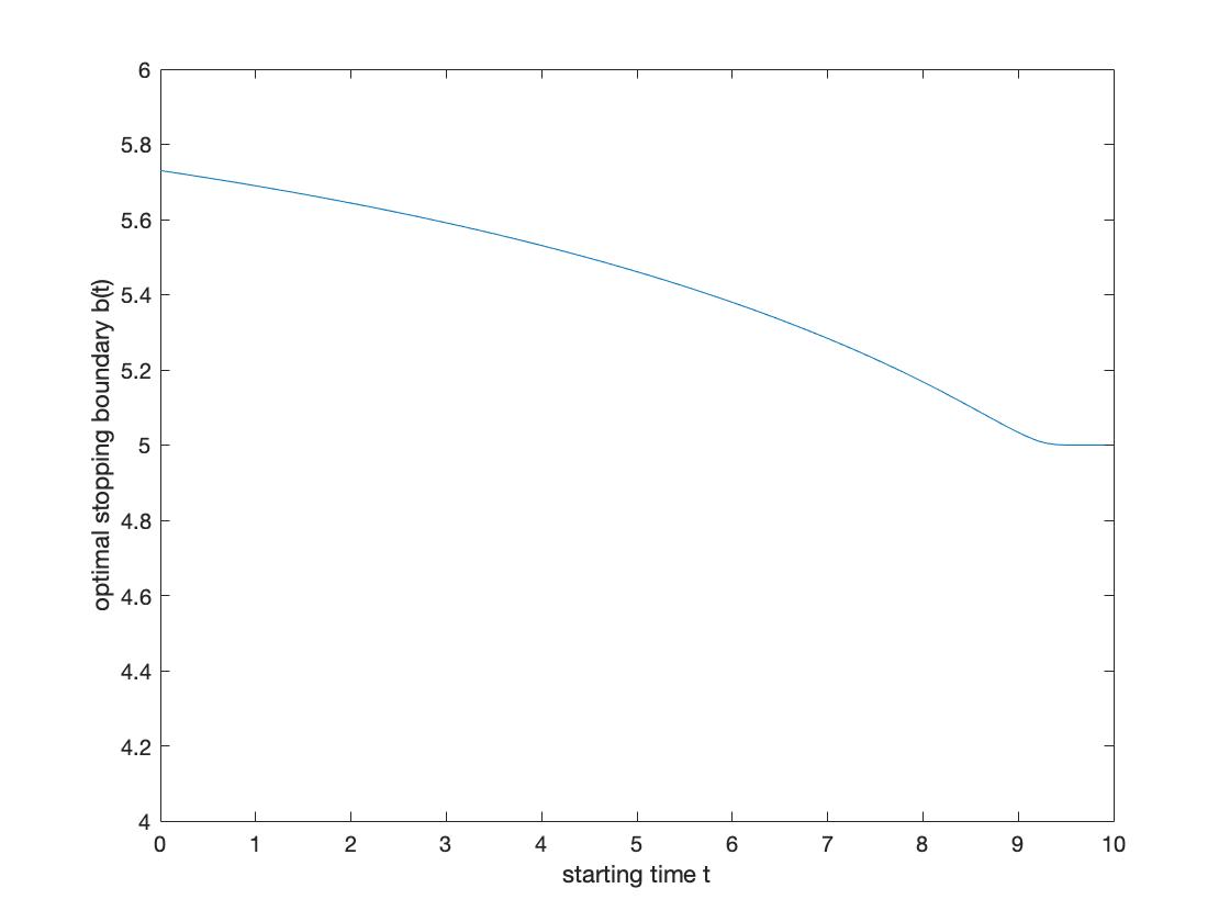
Figure 2: This figure displays the maps $t\mapsto b(t)$ with chosen parameters $r=0.02$, $\sigma=0.3$, $\lambda=0.4$, $L=5$ and $T=10$.

Remark 4.4.

Figure 2 seemingly has a flat tail for $t\in[9.5,10]$, this is because the plot function in Matlab has automatically rounded the number to $4$ decimal places; but if vpa function is used to recover their values, we see that

$$b(9.5)\approx 5.0011848117586090722852532053366,$$

$$b(9.6)\approx 5.0001059441386450643562966433819,$$

$$b(9.7)\approx 5.0000008520428087521736415510532,$$

$$b(9.8)\approx 5.0000000000049764636855798016768.$$

Appendix A Computations Associated with Azéma Supermartingale

1. For notational convenience, we set:

$$\alpha=\frac{2r}{\sigma^{2}}-1,\qquad b=r-\frac{\sigma^{2}}{2}$$

$$m=-\frac{d_{1}^{2}}{2},\qquad n=-\frac{d_{2}^{2}}{2}$$

$$d_{1}=-\log y{\sigma}^{-1}(T-t)^{-\frac{1}{2}}+b\sigma^{-1}(T-t)^{\frac{1}{2}}$$

$$d_{2}=-\log y{\sigma}^{-1}(T-t)^{-\frac{1}{2}}-b\sigma^{-1}(T-t)^{\frac{1}{2}}$$

$$\frac{\partial d_{1}}{\partial t}=-\frac{\log y}{2\sigma}(T-t)^{-\frac{3}{2}}-\frac{b}{2\sigma}(T-t)^{-\frac{1}{2}}$$

$$\frac{\partial d_{2}}{\partial t}=-\frac{\log y}{2\sigma}(T-t)^{-\frac{3}{2}}+\frac{b}{2\sigma}(T-t)^{-\frac{1}{2}}$$

$$\frac{\partial d_{1}}{\partial y}=\frac{\partial d_{2}}{\partial y}=-\sigma^{-1}y^{-1}(T-t)^{-\frac{1}{2}}$$

$$\left(\frac{\partial d_{1}}{\partial y}\right)^{2}=\left(\frac{\partial d_{2}}{\partial y}\right)^{2}=\sigma^{-2}y^{-2}(T-t)^{-1}$$

$$\frac{\partial^{2}d_{1}}{\partial y^{2}}=\frac{\partial^{2}d_{2}}{\partial y^{2}}=\sigma^{-1}y^{-2}(T-t)^{-\frac{1}{2}}$$

2. The derivative of $Z$ w.r.t time $t$:

$$\frac{\partial Z}{\partial t}(t,y) =\frac{1}{\sqrt{2\pi}}\left(e^{m}\frac{\partial d_{1}}{\partial t}+y^{\alpha}e^{n}\frac{\partial d_{2}}{\partial t}\right)$$

$$=\frac{1}{\sqrt{8\pi}}\left(-e^{m}\sigma^{-1}(T-t)^{-\frac{3}{2}}\log{y}-e^{n}\sigma^{-1}(T-t)^{-\frac{3}{2}}y^{\alpha}\log{y}\right).$$ (A.78)

3. The derivative of $Z$ w.r.t. space $y$:

$$\frac{\partial Z}{\partial y}(t,y) =\frac{1}{\sqrt{2\pi}}\left(e^{m}\frac{\partial d_{1}}{\partial y}+\alpha y^{\alpha-1}\Phi(d_{2})+y^{\alpha}e^{n}\frac{\partial d_{2}}{\partial y}\right)$$

$$=\frac{1}{\sqrt{2\pi}}\left(-\sigma^{-1}y^{-1}(T-t)^{-\frac{1}{2}}\left(y^{\alpha}e^{n}+e^{m}\right)+\alpha y^{\alpha-1}\Phi(d_{2})\right).$$ (A.79)

4. The derivative is bounded for $y>L>1$ and $t\in[0,T]$:

$$\bigg{|}\frac{\partial Z}{\partial y}(t,y)\bigg{|} =\sqrt{\frac{2}{\pi}}\sigma^{-1}y^{-1}(T-t)^{-\frac{1}{2}}e^{-\frac{d_{1}^{2}}{2}}-\alpha y^{\alpha-1}\Phi(d_{2})$$

$$\leq\sqrt{\frac{2}{\pi}}\sigma^{-1}(T-t)^{-\frac{1}{2}}e^{-\frac{d_{1}^{2}}{2}}-\alpha$$

$$\leq\sqrt{\frac{2}{\pi}}\sigma^{-1}(T-t)^{-\frac{1}{2}}e^{-\frac{\left(-\log L{\sigma}^{-1}(T-t)^{-\frac{1}{2}}-b\sigma^{-1}(T-t)^{\frac{1}{2}}\right)^{2}}{2}}-\alpha=C_{1}<\infty.$$ (A.80)

Note that for $t\to T$, but observe that as $\left(T-t\right)^{-\frac{1}{2}}\to\infty$, $e^{-\frac{d_{1}^{2}}{2}}\to-\infty$ which is decreasing much faster.

5. Useful Results for the Proof of Smooth-fit Condition

Lemma A.1 (For Chapter 4).

As $\epsilon\to 0$, $\tau_{\epsilon}\to 0$ almost surely.

Proof.

By construction of $\tau_{\epsilon}$ and the definition of $Y$,

$$\tau_{\epsilon} =\inf\{0\leq s\leq T-t:Y_{t+s}^{y-\epsilon}\geq b(t+s)\}$$

$$=\inf\bigg{\{}0\leq s\leq T-t:\frac{(y-\epsilon)\vee S_{s}}{X_{s}}\geq b(t+s)\bigg{\}}.$$

Note that $\bigg{\{}\frac{y-\epsilon}{X_{s}}\geq b(t+s)\bigg{\}}\subseteq\bigg{\{}\frac{(y-\epsilon)\vee S_{s}}{X_{s}}\geq b(t+s)\bigg{\}}$ so that

$$\tau_{\epsilon}\leq\hat{\tau}_{\epsilon} =\inf\bigg{\{}0\leq s\leq T-t:\frac{y-\epsilon}{X_{s}}\geq b(t+s)\bigg{\}}$$

$$=\inf\bigg{\{}0\leq s\leq T-t:(y-\epsilon)e^{-\left(r+\frac{\sigma^{2}}{2}\right)s-\sigma\widetilde{W}_{s}}\geq b(t+s)\bigg{\}}$$

$$=\inf\bigg{\{}0\leq s\leq T-t:-\widetilde{W}_{s}\geq\frac{\log{\frac{b(t+s)}{y-\epsilon}}+\left(r+\frac{\sigma^{2}}{2}\right)s}{\sigma}\bigg{\}}.$$

Let $\beta=r+\frac{\sigma^{2}}{2}$ and $g(s)=\frac{\log{\frac{b(t+s)}{y-\epsilon}}+\beta s}{\sigma}$ for notational convenience. As $\epsilon\to 0$, (recalling that $y=b(t)$),

$$g(s)\to\frac{\log{\frac{b(t+s)}{b(t)}}+\beta s}{\sigma}\leq\frac{\beta s}{\sigma},$$

where the inequality follows from the map $t\mapsto b(t)$ being decreasing, and since $s\mapsto\frac{\beta s}{\sigma}$ is a lower function for standard Brownian motion $\widetilde{W}$ under measure $\widetilde{P}$, so is $g(s)$, implying that $\widetilde{P}(\hat{\tau}_{\epsilon}=0)=1$, together with the fact that $0\leq\tau_{\epsilon}\leq\hat{\tau}_{\epsilon}=0$ a.s, we know $\tau_{\epsilon}=0$ a.s. ∎

6. Property of the Value Function

Lemma A.2.

The map $t\mapsto V(t,y)$ is decreasing.

Proof.

By the time-homogeneous property of process $Y$, for $\tau\in[0,T-t]$,

$$\widetilde{E}_{t,y}\left(e^{-\lambda\tau}\left(Y_{t+\tau}-L\right)^{+}Z\left(t+\tau,Y_{t+\tau}\right)\right)=\widetilde{E}\left(e^{-\lambda\tau}\left(Y_{\tau}^{y}-L\right)^{+}Z\left(t+\tau,Y_{\tau}^{y}\right)\right),$$

and since the map $t\mapsto Z(t,y)$ is decreasing, we have $t\mapsto\widetilde{E}\left(e^{-\lambda\tau}\left(Y_{\tau}^{y}-L\right)^{+}Z\left(t+\tau,Y_{\tau}^{y}\right)\right)$ is decreasing. Moreover, $t\mapsto T-t$ is decreasing so that the supremum is taken over a smaller set as $t$ increases and that by definition, $t\mapsto V(t,y)$ is decreasing. ∎

7. The second derivative of $Z$ w.r.t space $y$:

$$\frac{\sigma^{2}y^{2}}{2}\frac{\partial^{2}Z}{\partial y^{2}}(t,y) =\frac{1}{\sqrt{8\pi}}\sigma^{2}y^{2}\left(-d_{1}e^{m}\left(\frac{\partial d_{1}}{\partial y}\right)^{2}+e^{m}\frac{\partial^{2}d_{1}}{\partial y^{2}}+\alpha(\alpha-1)y^{\alpha-2}\Phi(d_{2})\right.$$

$$\qquad\qquad\qquad\,\,\,\,\,\left.+\alpha y^{\alpha-1}e^{n}\frac{\partial d_{2}}{\partial y}-d_{2}y^{\alpha}e^{n}\left(\frac{\partial d_{2}}{\partial y}\right)^{2}+y^{\alpha}e^{n}\frac{\partial^{2}d_{2}}{\partial y^{2}}\right)$$

$$=\frac{1}{\sqrt{8\pi}}\left(-d_{1}e^{m}(T-t)^{-1}+e^{m}\sigma(T-t)^{-\frac{1}{2}}+\alpha(\alpha-1)\sigma^{2}y^{\alpha}\Phi(d_{2})\right.$$

$$\qquad\qquad\left.-2\alpha\sigma y^{\alpha}e^{n}(T-t)^{-\frac{1}{2}}-d_{2}y^{\alpha}e^{n}(T-t)^{-1}+y^{\alpha}e^{n}\sigma(T-t)^{-\frac{1}{2}}\right).$$

8. The Uniform Integrability of $Y$

To apply the dominated convergence theorem, we observe that

$$Y_{t}^{y} =\frac{y\vee\max\limits_{0\leq{u}\leq t}X_{u}}{X_{t}}\leq\frac{y\max\limits_{0\leq{u}\leq T}X_{u}}{X_{t}}=ye^{-(r+\frac{\sigma^{2}}{2})t-\sigma\widetilde{W}_{t}}\max\limits_{0\leq{u}\leq T}X_{u}$$

$$\leq ye^{\sigma\max\limits_{0\leq{u}\leq T}(-\widetilde{W}_{u})}e^{\left(r+\frac{\sigma^{2}}{2}\right)T+\sigma\max\limits_{0\leq{u}\leq T}(\widetilde{W}_{u})}$$

$$\leq\frac{1}{2}ye^{\left(r+\frac{\sigma^{2}}{2}\right)T}\left(e^{2\sigma\max\limits_{0\leq u\leq T}(-\widetilde{W}_{u})}+e^{2\sigma\max\limits_{0\leq u\leq T}\widetilde{W}_{u}}\right){\buildrel d\over{=}}\,ye^{\left(r+\frac{\sigma^{2}}{2}\right)T}e^{2\sigma\sqrt{T}X},$$ (A.81)

where the first inequality holds as $y\geq 1$, $\max\limits_{0\leq{u}\leq T}X_{u}\geq\max\limits_{0\leq{u}\leq t}X_{u}\geq 1$ and the last inequality follows from Young’s inequality and the random variable $X$ has the probability density function given as follows

$$f_{X}(x) =\sqrt{\frac{2}{\pi}}e^{-\frac{x^{2}}{2}},\qquad x>0.$$

We further estimate the following

$$\widetilde{E}\left(e^{2\sigma\sqrt{T}X}\right) =\sqrt{\frac{2}{\pi}}\int_{0}^{\infty}e^{2\sigma\sqrt{T}x-\frac{x^{2}}{2}}dx$$

$$=\sqrt{\frac{2}{\pi}}\int_{0}^{\infty}e^{-\frac{1}{2}\left(x^{2}-4\sigma\sqrt{T}x+4\sigma^{2}T\right)+2\sigma^{2}T}dx$$

$$=\sqrt{\frac{2}{\pi}}e^{2\sigma^{2}T}\int_{-2\sigma\sqrt{T}}^{\infty}e^{-\frac{y^{2}}{2}}dy\qquad\text{ (Change of variable $y=x-2\sigma\sqrt{T}$)}$$

$$=e^{2\sigma^{2}T}+\sqrt{\frac{2}{\pi}}e^{2\sigma^{2}T}\int_{-2\sigma\sqrt{T}}^{0}e^{-\frac{y^{2}}{2}}dy<\infty.$$

We therefore, in a somewhat lengthy way, have proven that $Y_{t}^{y}$ is dominated by a positive integrable random variable.

References

- [1] Du Toit, J., Peskir, G. and Shiryaev, A.N., 2008. Predicting the last zero of Brownian motion with drift. Stochastics: An International Journal of Probability and Stochastics Processes, 80(2-3), pp.229-245.
- [2] Du Toit, J. and Peskir, G., 2009. Selling a stock at the ultimate maximum. The Annals of Applied Probability, 19(3), pp.983-1014.
- [3] Gapeev, P.V. and Li, L., 2022. Optimal stopping problems for maxima and minima in models with asymmetric information. Stochastics, 94(4), pp.602-628.
- [4] Ghomrasni, R. and Peskir, G., 2004. Local time-space calculus and extensions of Itô’s formula. In High Dimensional Probability III (pp. 177-192). Birkhäuser, Basel.
- [5] Glover, K., Peskir, G. and Samee, F., 2011. The British Russian Option. Stochastics An International Journal of Probability and Stochastic Processes, 83(4-6), pp.315-332.
- [6] Hull, J. and White, A., 1995. The impact of default risk on the prices of options and other derivative securities. Journal of Banking and Finance, 19(2), pp.299-322.
- [7] Mansuy, R. and Yor, M., 2006. Random times and enlargements of filtrations in a Brownian setting (Vol. 1873). Berlin: Springer.
- [8] Meyer, P.A., Smythe, R.T. and Walsh, J.B., 1972, January. Birth and death of Markov processes. In Proceedings of the Sixth Berkeley Symposium on Mathematical Statistics and Probability (Vol. 3, pp. 295-305).
- [9] Elliott, R.J., Jeanblanc, M. and Yor, M., 2000. On models of default risk. Mathematical Finance, 10(2), pp.179-195.
- [10] Nikeghbali, A., 2006. An essay on the general theory of stochastic processes. Probability Surveys, 3, pp.345-412.
- [11] Peskir, G. and Shiryaev, A., 2006. Optimal stopping and free-boundary problems (pp. 123-142). Birkhäuser Basel.
- [12] Peskir, G., 2005. A change-of-variable formula with local time on curves. Journal of Theoretical Probability, 18(3), pp.499-535.
- [13] Peskir, G., 2007. A change-of-variable formula with local time on surfaces. In Séminaire de probabilités XL (pp. 70-96). Springer, Berlin, Heidelberg.
- [14] Shepp, L. and Shiryaev, A.N., 1993. The Russian option: reduced regret. The Annals of Applied Probability, 3(3), pp.631-640.
- [15] Shepp, L.A. and Shiryaev, A.N., 1995. A new look at pricing of the” Russian option “. Theory of Probability and Its Applications, 39(1), pp.103-119.
- [16] Shiryaev, A.N., 1999. Essentials of stochastic finance: facts, models, theory (Vol. 3). World scientific.