Removal of point source leakage from time-order data filtering

Abstract

Time-ordered data (TOD) from ground-based CMB experiments are generally filtered before map-making to remove or reduce the contamination from the ground and the atmospheric emissions. However, when the observation region contains strong point sources, the filtering process will result in considerable leakage around the point sources in a measured CMB map, and leave spurious polarization signals. Therefore, such signals need to be assessed and removed before CMB science exploitation. In this work, we present a new method that we call ”template fitting” and can effectively remove these leakage signals in pixel domain, not only satisfying the requirement for measuring primordial gravitational waves from CMB-$B$ modes, but also avoiding time-consuming operations on TOD.

1 Introduction

The cosmic microwave background (CMB) temperature and polarization anisotropies are strong observational evidence of the inflationary expansion history of the Universe. Especially, the detection of $B$-mode CMB polarization in form of the tensor to scalar ratio $r$ is crucial for confirming the existence of the gravitational waves in the early Universe, which is a natural consequence of the inflationary potential. Several space and ground-based experiments are devoted to constraining $r$, including the BICEP series [1], Planck [2], QUIJOTE [3], ACTPol [4], SPTPol [5]. Current observations already limit the tensor to scalar ratio to $r\leq 0.036-0.1$ [6, 7, 8, 9, 10], and the forthcoming experiments including POLARBEAR [11], LiteBIRD [12], CMB-S4 [13], the Simons Observatory [14], and AliCPT [15] will devote to reaching a sensitivity of $r=0.001$. This inevitably requires dedicated treatments of all kinds of contamination and systematics. Especially, all available CMB experiments in the next $5\sim 10$ years are ground-based, which are ineluctably contaminated by the atmosphere and ground emissions. Therefore, their time-order data (TOD) needs to be filtered to alleviate these contaminations.

Usually, in a ground-based experiment (e.g., BICEP or AliCPT), the observed TOD is converted to the T, Q, and U maps by the data analysis pipeline that contains data splitting and cutting, pointing and polarization orientation reconstruction (for each detector), time domain filtering, and the final time-to-pixel domain map making. First of all, the TOD are split in units of “halfscan”, and “scanset” (tens of neighbouring halfscans), and bad data are removed at certain thresholds. After that, the pointing trajectory and polarization orientation for each detector are constructed from the encoder data, GPS time, site location as well as the focal plane structure, then the TOD are high-passed to suppress long-distance correlations arising from noise sources or systematic errors. In order to remove the atmospheric radiation present in the data, a polynomial filter (typically of the 3rd order) is applied, and to handle noise associated with the ground coordinate system, such as ground reflections/emissions, templates are constructed and removed for each scanset, which is called a ground subtraction filter. In addition, as a polarization experiment targeting the CMB $B$-mode, the temperature-polarization leakages need to be removed as much as possible, e.g., by using a de-projection filter on scansets to suppress the leakage due to the beam mismatch of orthogonal polarization detector pairs. It is worth noting that all the filters mentioned above are linear, so it is possible to implement them either as direct time domain operations, or as pixel domain matrix operations, which are completely equivalent. After all these operations, the TOD is weighted by the inverse variance estimated from each scanset, and then projected and co-added on the sky for each map pixel, to produce the final observed map.

Unfortunately, although the TOD filtering can efficiently remove the atmosphere/ground emissions, as well as fixing some other errors, it will also remove part of the CMB signal and cause leakages from point sources to the pixel domain regions around them. Because the latter usually has no preference for the $E$- and $B$-modes, when the point source is strong, it can significantly contaminate the weak primordial $B$-mode signal in a large pixel domain region. For measuring the primordial gravitational waves through the extremely faint $B$-mode signal, this kind of leakage has to be removed accurately.

In principle, if one knows the positions of point sources, then it is possible to identify their locations in TOD and cut the corresponding TOD segments to prevent the leakage due to filtered point sources. However, this will cause several problems: 1) Not all point sources are strong enough to be identified from the TOD, because the TOD is much noisier than the final stacked sky map. 2) Removal of the TOD segments with the point source will break the integrity of the TOD and cause inconvenience and issues in filtering and map-making. 3) Typically, operations on TOD are very time-consuming, so removal of the point source leakage directly in the TOD becomes in feasible in practice.

In this work, we introduce a new method to remove the point source leakage due to filtering of the TOD. This method is based on  [16] and operates mainly in the pixel domain. The main idea is to construct ideal and realistic templates of the leakages in the pixel domain, and then remove the leakages by linear regression. The advantage of this method is obvious: 1) This method will not cut the TOD, which is safe, convenient and friendly to all types of TOD operations. 2) From the test results, this method can successfully remove the point source leakage down to the level satisfying the detection requirement of $r\leq 0.001$. 3) This method operates mainly in the pixel domain, which is fast and easy to implement.

The structure of this paper is as follows: in Sect. 2, we introduce our removal of point source leakage method for both single and multiple point sources. We give examples for these two situations and use actual point sources data to verify our method in Sect. 3. Finally, we summarize and conclude in Sect. 4.

2 Methods

The core concept to alleviate the point source leakages on the final sky map is based on the fact, that all TOD operations and their effects in the pixel domain sky maps are linear. In order to remove the leakages by linear regression, the fundamental operation is to create pixel domain leakage templates. Since the data we obtain from the pipeline is always filtered, two types of templates can be produced: ideal and realistic. The main difference between them is that the ideal template requires complete knowledge of the beam profile, which is usually unavailable; whereas a realistic template is constructed directly from the product of the pipeline, which is always available. Certainly, the performance of the ideal template is better than the realistic template, as we will mention below that the results of cleaning by the realistic template are also acceptable.

2.1 The ideal template

Construction of the ideal template is straightforward: the filtered sky map $\bm{D^{\prime}}$ produced by the pipeline is

$$\bm{D^{\prime}}=(\bm{I}-\bm{M})\cdot\bm{F}\cdot(\bm{d}+\bm{d}_{p}),$$ (2.1)

where $\bm{d}_{p}$ is a single point source (assumed to have Gaussian shape in simulation) and

$$\bm{d}=\bm{d}_{c}+\bm{d}_{f}+\bm{n}$$ (2.2)

is a column vector containing the input signals other than the point sources: $\bm{d}_{c}$ is the CMB signal, $\bm{d}_{f}$ is the foreground, and $\bm{n}$ is the noise. $\bm{F}$ is a square matrix representing the linear filtering effect. $\bm{M}$ is a diagonal matrix for the point source mask, which is 1 for the region around the point source and 0 elsewhere, and $\bm{I}$ is the identity matrix. Thus, $\bm{I}-\bm{M}$ is the non-point source region where the point source leakages need to be studied. For convenience, the filtered result of $\bm{d}$ is also computed as

$$\bm{d^{\prime}}=(\bm{I}-\bm{M})\cdot\bm{F}\cdot\bm{d}.$$ (2.3)

Note that both $\bm{d}$ and $\bm{d}^{\prime}$ are without the point source or point source leakages.

It is clear from the descriptions above that the ideal template $\bm{\mathcal{T}}_{0}$ is

$$\bm{\mathcal{T}}_{0}=(\bm{I}-\bm{M})\cdot\bm{F}\cdot\bm{d}_{p},$$ (2.4)

which fully contains the point source leakage due to filtering except for an unknown point source amplitude. If the amplitude of the template can be perfectly determined, then we have

$$\bm{D^{\prime}}=\bm{d^{\prime}}+\bm{\mathcal{T}}_{0},$$ (2.5)

which separates the signal and point source leakages completely. In practice, the amplitude of the template should be determined by linear regression, and the best-fit template is subtracted to remove the point source leakage, leaving a residual that is no more than the chance correlation between $\bm{\mathcal{T}}_{0}$ and $\bm{d}^{\prime}$, whose amplitude is typically a few percent of $\bm{d}^{\prime}$.

2.2 The realistic template

The ideal template can remove the point source leakages more effectively, but it necessitates precise knowledge of the beam profile, including the asymmetry, which is usually unavailable. Therefore, we go forward with creating a realistic template that can be obtained directly from the sky map produced by the pipeline. The main idea to construct the realistic template is based on three reasonable assumptions:

1. The point sources are almost unaffected by the TOD filtering. This is true according to [17], which shows the small scale structures are almost unaffected by the TOD filtering.

2. The point source mask is big enough to include the majority of the point source. According to [18, 19], the FWHM of AliCPT beam varies from $12^{\prime}\sim 19^{\prime}$, which corresponds to the Gaussian beam width of $\sigma<10^{\prime}$. Therefore, a mask of $r=40^{\prime}$ region is enough to exclude most point sources, with an exception of a few extremely bright sources along the Galactic plane.

3. The point source is significantly stronger than the CMB/foreground at the position of itself. Although it is possible to detect point sources that are weaker than the CMB, the leakages produced by these point sources are negligible, thus their leakages don’t need to be taken into account.

With assumption 1, it is easy to see that $\bm{d}_{p}\approx\bm{F}\cdot\bm{d}_{p}$, and assumption 2 ensures $\bm{d}_{p}\approx\bm{M}\cdot\bm{d}_{p}$; thus, we have:

$$\bm{d}_{p}\approx\bm{M}\cdot\bm{F}\cdot\bm{M}\cdot\bm{d}_{p}$$ (2.6)

Substitute the above one into Eq. 2.5, we get the realistic template $\bm{\mathcal{T}}_{1}$ as:

$$\bm{\mathcal{T}}_{1}=(\bm{I}-\bm{M})\cdot\bm{F}\cdot(\bm{M}\cdot\bm{F}\cdot\bm{M}\cdot\bm{d}_{p})\approx\bm{\mathcal{T}}_{0}$$ (2.7)

The above equation is crucial, because $(\bm{M}\cdot\bm{F}\cdot\bm{M}\cdot\bm{d}_{p})$ is the sky map produced by the pipeline with a point source mask $\bm{M}$. Thus, no need for us to know the details of the beam profile, and $\bm{\mathcal{T}}_{1}$ can be obtained by feeding the sky map product of the pipeline (with a proper point source mask applied) into the pipeline again as $\bm{F}\cdot(\bm{M}\cdot\bm{F}\cdot\bm{M}\cdot\bm{d}_{p})$.

2.3 Other procedures

The aforementioned method is firstly tested using a single point source simulation. First, Eq. 2.1 constructs the filtered sky map, and Eqs. 2.5& 2.7 provide the ideal and realistic templates $\bm{\mathcal{T}}_{0}$ and $\bm{\mathcal{T}}_{1}$, respectively. If the polarization direction of a point source is already known, since the leakage is caused by both of Q and U in the pipeline, a fitting parameter $k$ for both of Q and U is determined using linear regression to minimize the RMS (root-mean-square) of residual. Here the RMS of residual is:

$$(\sigma^{Q}_{\xi})^{2} =\frac{1}{n}\left[\sum_{i=1}^{n}(\bm{D^{\prime}}-k_{\xi}\cdot\bm{\mathcal{T}}_{\xi})^{2}_{i}\right]_{Q}\,,$$ (2.8)

$$(\sigma^{U}_{\xi})^{2} =\frac{1}{n}\left[\sum_{i=1}^{n}(\bm{D^{\prime}}-k_{\xi}\cdot\bm{\mathcal{T}}_{\xi})^{2}_{i}\right]_{U}\,,$$

$$\sigma^{2}_{\xi} =(\sigma^{Q}_{\xi})^{2}+(\sigma^{U}_{\xi})^{2}$$

where $i$ is pixel number, $n$ is the total number of pixels, the superscripts $Q$ and $U$ of $\sigma$ denote the Stokes parameters, the subscript $Q$ or $U$ on the right term stands for the Stokes parameter vector solely considered in this formula, and $\xi=0,1$ for the ideal or realistic templates respectively.

If the point source’s polarization direction is unknown, we construct separately $\bm{\mathcal{T}}^{Q}$ and $\bm{\mathcal{T}}^{U}$, whose input only contains values for $Q$ (or $U$) Stokes parameter vector. Multi-linear regression should be applied to simultaneously determine $k^{Q}$ and $k^{U}$ in order to minimize the RMS of residual in the pixel domain. This is because the filtering calculation will mix the Q and U Stokes parameter, and $\bm{\mathcal{T}}^{Q}$ (or $\bm{\mathcal{T}}^{U}$) is not zero on $U$-part (or $Q$-part) even for a $Q$-only (or $U$-only) input. Hence for each of the Stokes parameters, the RMS of the residual is as follows:

$$(\sigma_{\xi}^{Q})^{2} =\frac{1}{n}\left[\sum_{i=1}^{n}(\bm{D^{\prime}}-k_{\xi}^{Q}\cdot\bm{\mathcal{T}}_{\xi}^{Q}-k_{\xi}^{U}\cdot\bm{\mathcal{T}}_{\xi}^{U})^{2}_{i}\right]_{Q}\,,$$ (2.9)

$$(\sigma_{\xi}^{U})^{2} =\frac{1}{n}\left[\sum_{i=1}^{n}(\bm{D^{\prime}}-k_{\xi}^{Q}\cdot\bm{\mathcal{T}}_{\xi}^{Q}-k_{\xi}^{U}\cdot\bm{\mathcal{T}}_{\xi}^{U})^{2}_{i}\right]_{U}\,,$$

$$\sigma_{\xi}^{2} =(\sigma_{\xi}^{Q})^{2}+(\sigma_{\xi}^{U})^{2}$$

where the Stokes parameter vector is solely taken into account in the formula by the subscript $Q$ (or $U$) of the right term.

We also test our method with multiple point sources. The filtered sky map $\bm{D^{\prime}}$ is shown here as follows:

$$\bm{D^{\prime}}=(\bm{I}-\bm{M}_{\Sigma})\cdot\bm{F}\cdot(\bm{M}_{\Sigma}\cdot\sum_{j}\bm{d}_{p,j}+\bm{d})\,,$$ (2.10)

where $j$ is the index of point source, $\bm{M}_{\Sigma}=\sum_{j}\bm{M}_{j}$ is the mask for all point sources and $\bm{M}_{j}$ is the $j^{th}$ single point source mask, and $\bm{I}-\bm{M}_{\Sigma}$ is the non-point source region to investigate the impact of leakage. Hence the ideal and realistic templates for each point source are:

$$\bm{\mathcal{T}}_{0,j} =(\bm{I}-\bm{M}_{\Sigma})\cdot\bm{F}\cdot\bm{M}_{j}\cdot\bm{d}_{p,j}\,,$$ (2.11)

$$\bm{\mathcal{T}}_{1,j} =(\bm{I}-\bm{M}_{\Sigma})\cdot\bm{F}\cdot(\bm{M}_{j}\cdot\bm{F}\cdot\bm{M}_{j}\cdot\bm{d}_{p,j})$$

Correspondingly, the fitting parameters $k_{\xi j}$ (when the polarization direction is known) or $k_{\xi j}^{Q}$ and $k_{\xi j}^{U}$ (when the polarization direction is unknown) are computed for each point source using a multi-linear regression that takes into account all the templates simultaneously, in order to minimize the RMS of residuals in the combined non-point sources region. If the polarization directions of point sources are already known, then the RMS are:

$$(\sigma_{\xi}^{Q})^{2} =\frac{1}{n}\left[\sum_{i=1}^{n}(\bm{D^{\prime}}-\sum_{j}k_{\xi j}\bm{\mathcal{T}}_{\xi j})^{2}_{i}\right]_{Q}\,,$$ (2.12)

$$(\sigma_{\xi}^{U})^{2} =\frac{1}{n}\left[\sum_{i=1}^{n}(\bm{D^{\prime}}-\sum_{j}k_{\xi j}\bm{\mathcal{T}}_{\xi j})^{2}_{i}\right]_{U}\,,$$

$$\sigma^{2}_{\xi} =(\sigma_{\xi}^{Q})^{2}+(\sigma_{\xi}^{U})^{2}$$

and if the polarization directions are unknown, then the RMS are:

$$(\sigma_{\xi}^{Q})^{2} =\frac{1}{n}\left[\sum_{i=1}^{n}(\bm{D^{\prime}}-\sum_{j}k_{\xi j}^{Q}\bm{\mathcal{T}}_{\xi j}^{Q}-\sum_{j}k_{\xi j}^{U}\bm{\mathcal{T}}_{\xi j}^{U})^{2}_{i}\right]_{Q}\,,$$ (2.13)

$$(\sigma_{\xi}^{U})^{2} =\frac{1}{n}\left[\sum_{i=1}^{n}(\bm{D^{\prime}}-\sum_{j}k_{\xi j}^{Q}\bm{\mathcal{T}}_{\xi j}^{Q}-\sum_{j}k_{\xi j}^{U}\bm{\mathcal{T}}_{\xi j}^{U})^{2}_{i}\right]_{U}\,,$$

$$\sigma^{2}_{\xi} =(\sigma_{\xi}^{Q})^{2}+(\sigma_{\xi}^{U})^{2}$$

3 Simulations and tests

In the computation that follows, we use the outcome with the local monopoles subtracted from each Stokes parameter in the non-point source region, in order to demonstrate the method’s ability to correct the leakages. To reduce accidental fluctuation, we also use 10 different CMB and noise realizations in the simulation.

After determining the fitting parameters by multi-linear regression, we build dB ($20\log_{10}P$) sky maps of the two templates, their residuals and compute the dB effect to compare the degree of correction in the pixel domain. All these dB maps are computed from the polarization intensity $P$.

The residual map is the difference between the filtered sky map (no leakage effect from the beginning) and cleaned sky map. When the polarization directions are already known, the residual map is:

$$\bm{\delta}_{\xi}=\left(\bm{D^{\prime}}-\sum_{j}k_{\xi j}\bm{\mathcal{T}}_{\xi j}\right)-\bm{d^{\prime}}\,,$$ (3.1)

and when the polarization direction is unknown, the residual is:

$$\bm{\delta}_{\xi}=\left(\bm{D^{\prime}}-\sum_{j}k^{Q}_{\xi j}\bm{\mathcal{T}}^{Q}_{\xi j}-\sum_{j}k^{U}_{\xi j}\bm{\mathcal{T}}^{U}_{\xi j}\right)-\bm{d^{\prime}}\,,$$ (3.2)

where $\xi=0,1$ for the ideal and realistic templates, respectively. Now we introduce a quantity, $\bm{E}^{\rm dB}_{\xi,P}$, dubbed as ”dB effect”, for easily comparing the residuals with respect to the CMB in units of $\rm dB$, in the form of:

$$\bm{E}^{\rm dB}_{\xi,P}=20\log_{10}\dfrac{P_{\bm{\delta}}}{\langle P_{\rm cmb}\rangle}\,,$$ (3.3)

where the superscript $\rm dB$ stands for the units of decibels, and $P$ is the polarization intensity defined as $P=\sqrt{Q^{2}+U^{2}}$. $\langle P_{\rm cmb}\rangle$ is the mean value of CMB polarization intensity, about $2.070$ $\mu$K.

3.1 Single point source

For a single point source, the fitting parameter for the ideal template is very close to 1, whereas the fitting parameter for realistic template is above 1, because the amplitude of the point source is reduced by filtering. The fitting residuals are 1 to 2 orders of magnitudes less than the point source leakage template.

We select a location at $[b,l]=[50^{\circ},190^{\circ}]$, assuming that its polarization intensity is equal to $150$ $\mu K$. We then smooth this point by $19^{\prime}$ to make a Gaussian point source. We first assume that the polarization direction is already known, where we fix the polarization angle of this point source to be $22.5^{\circ}$, resulting in a Gaussian point source with the Q, U values of approximately $106$ $\mu$K. For this artificially point source, the fitting parameter with true leakage is close to 0.997 and polarization residual standard deviation is approximately $1.113\times 10^{-3}$ $\mu$K in the pixel domain. The fitting parameter with realistic template is close to 1.201, and the polarization residual standard deviation is roughly $1.999\times 10^{-3}$ $\mu$K in the pixel domain. Meanwhile, the true leakage and the realistic template have standard deviations of $0.028~{}\mu$K and $0.024~{}\mu$K for polarization, respectively. Additionally, after filtering calculation, polarization standard deviations of the CMB, foreground and noise are, in that order, $0.374$ $\mu$K, $0.027$ $\mu$K, and $0.121$ $\mu$K. After using our method for alleviating the impact of point source leakage, the standard deviation of residuals is consequently orders of magnitudes smaller than that of template we build, as well as smaller than that of CMB, foreground and noise. The impact of point source leakage is lessened by our correction method.

For a single Gaussian point source with a given polarization direction, we now present the polarization dB value of templates, residuals and dB effects, as illustrated in Fig. 1. The leakage of point source is diffused on the partial sky map after pipeline, as seen in the right column of Fig. 1, and it resembles a star. Although the residual’s amplitude is frequently lower than that of template, the residual also exhibits vivid spikes on the sky map (middle column). Additionally, dB effect shows the proportion between residual and mean CMB polarization. Realistic dB effect error is more than that of ideal dB effect (right column). Our method provides good accuracy in the case of single Gaussian point source because the residual left over after correction procedure is significantly less than the true leakage.

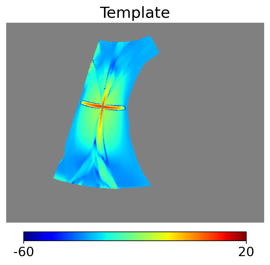
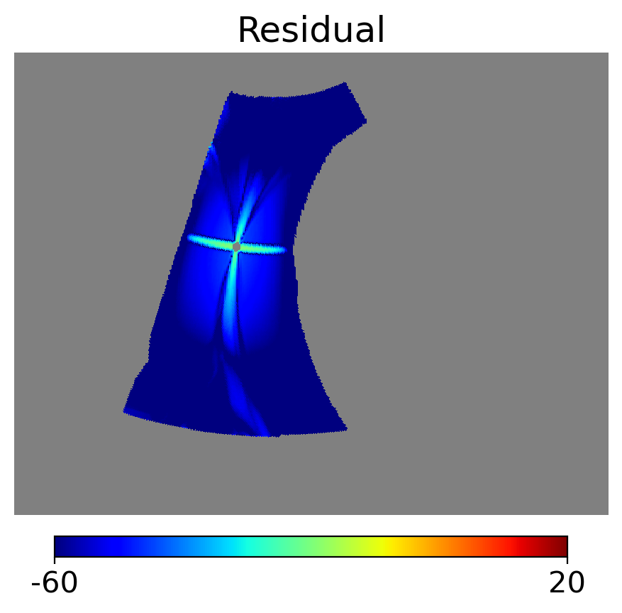
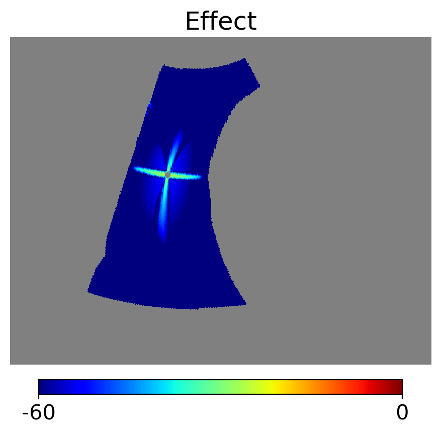
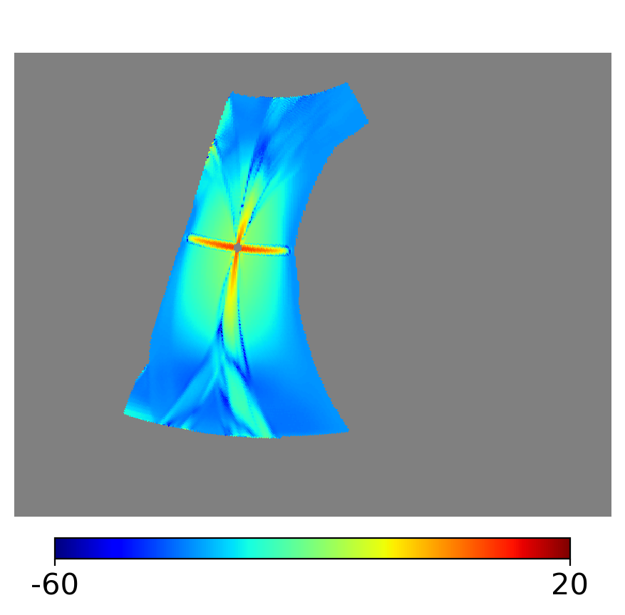
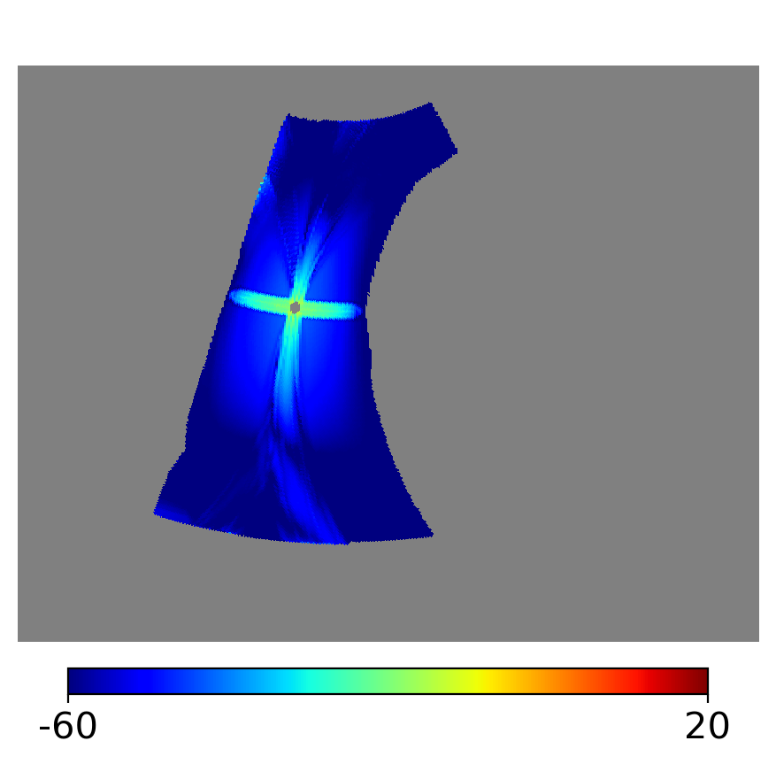
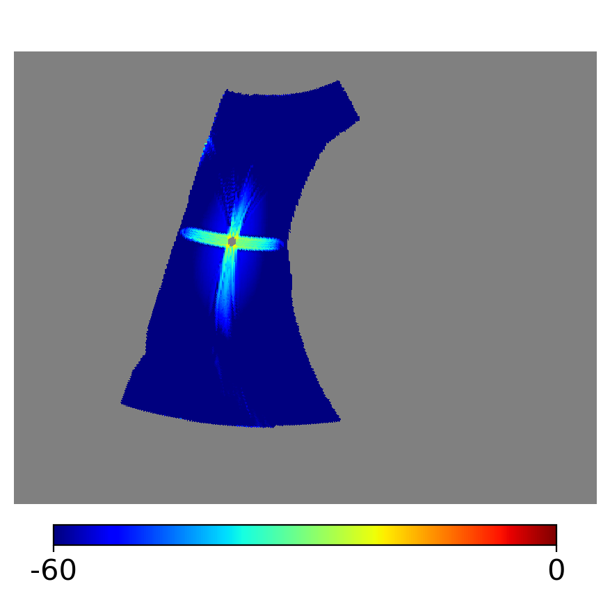
Figure 1: Comparison of results in units of decibels (dB), obtained using the ideal template (upper) and the realistic template (lower), for the case of a single point source with a given polarization direction, where the polarization values of the templates (left), the residuals (middle) from Eq. 3.1 and the dB effects (right) as defined in Eq. 3.3 are shown, respectively.

For single point source with known polarization direction, we compute the angular power spectrum of CMB, residual, and true leakage, as shown in Fig. 2. We select $\ell$ with a range of 20 to 700, because we only focus on part of the sky map. The residual spectra are 2 or 3 orders of magnitudes lower than that of the templates. For the $BB$ spectrum, the spectrum of residual is significantly smaller after our correction method than that of CMB. Hence our method can help to reduce the measurement error.

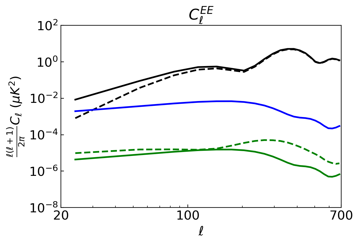
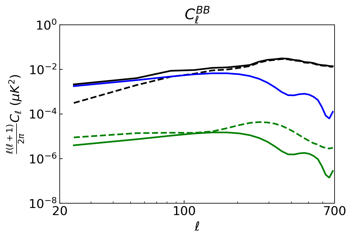
Figure 2: $EE$ and $BB$ power spectra for single point source with given polarization direction, including input (black solid) and filtered CMB (black dashed), residuals after the leakage removal for the ideal template (green solid) and the realistic template (green dashed), and the true leakage (blue).

The impact of unknown polarization direction is then verified in the case of single point source. On the basis that the polarization direction of this point source was known, the fitting parameter was previously determined. Assuming the point source’s polarization direction is unknown, the parameters are to be determined by fitting. We continue to construct the same ideal and realistic template as Eqs. 2.5& 2.7. For each type of template, $k^{U}/k^{Q}$ is equal to $\tan(2\theta)$ because that the filtering procedure is equivalent to linear matrix multiplication calculation. Taking $\theta=33.9^{\circ}$ as an example, the result of fitting parameters, residual standard deviations and the comparison of ratios under the condition of unknown polarization direction are presented in Tab. 1. For both ideal and realistic templates, $k^{U}/k^{Q}$ is nearly equal to $\tan(2\theta)$. The accuracy is affected to some extent by the CMB, foreground and noise due to the chance correlation. It demonstrates fitting parameters are still stable for the point source whose polarization direction is unknown.

Table 1: Derived fitting parameters for single point source with unknown polarization direction.

$k_{0}^{Q}$	$k_{0}^{U}$	$\sigma_{\delta_{0}}/10^{-3}\mu$K	$k_{1}^{Q}$	$k_{1}^{U}$	$\sigma_{\delta_{1}}/10^{-3}\mu$K	$k_{0}^{U}/k_{0}^{Q}$	$k_{1}^{U}/k_{1}^{Q}$	$\tan(2\theta)$
0.534	1.303	2.047	0.645	1.567	2.600	2.439	2.429	2.453

As a result of filtering calculation, there is a star-like leakage for a single Gaussian point source. Additionally, our approach can lower pixel domain error and make the residual spectrum much lower than the CMB spectrum. Furthermore, our method is still reliable and accurate even when the polarization direction of point source is unknown.

3.2 Multiple point sources

In the case of multiple point sources, the multi-linear regression method’s fitting parameters for each point source are comparable to the fitting results when each point source is treated as a single point source. The fitting residuals are still 1 to 2 orders of magnitudes less than the point source’s true leakages.

The same approach as the case of single point source is used on five point sources with random locations and smooth with $19^{\prime}$. Tab. 2 displays their locations and polarization amplitudes. For each point source, we construct accordingly the ideal and realistic templates. Under the assumption of given polarization direction, the fitting parameters for multiple point sources are given in Tab. 2, and are almost identical to the fitting parameters for each single point source, demonstrating the stability of our correction method for multiple point sources.

Table 2: Derived fitting parameters for multiple point sources by the multi-linear regression method when the polarization direction is known for each point source, which are comparable with those for each single point source.

Number	$[b,l]^{\circ}$	$P/\mu$K	$k_{0}$	$k_{1}$
1	[50, 190]	150	0.997	1.201
2	[27, 191]	200	0.995	1.187
3	[30, 173]	150	1.105	1.189
4	[39, 162]	120	1.021	1.199
5	[56, 160]	90	1.021	1.282

We also examine the influence of polarization direction of multiple point sources. In order to simulate a filtered sky map $\bm{D^{\prime}}$ for multiple point sources with unknown polarization directions, a series of polarizing angles $\theta_{j}$ are applied to the Stokes parameters of each individual point source $\bm{d}_{p,j}$ in Eq. 2.10, where $j$ is the index of each point source. The result of fitting parameters for multiple point sources with unknown polarization direction is provided in Tab. 3. The result is consistent with that for single point source. For each point source, the absolute values of $k^{Q}_{1}$ and $k^{U}_{1}$ are slightly higher than those of $k^{Q}_{0}$ and $k^{U}_{0}$ respectively, but $k^{U}/k^{Q}$ is still almost equal to $\tan(2\theta)$ for both the ideal and realistic templates, and the CMB, foreground, and noise still have a minor impact on the residual. Thus, for multiple point sources with unknown polarization direction, our method is still robust.

Table 3: Derived fitting parameters for multiple point sources with unknown polarization direction.

Number	$\theta^{\circ}$	$k_{0}^{Q}$	$k_{0}^{U}$	$k_{1}^{Q}$	$k_{1}^{U}$	$k_{0}^{U}/k_{0}^{Q}$	$k_{1}^{U}/k_{1}^{Q}$	$\tan(2\theta)$
1	33.9	0.535	1.304	0.646	1.568	2.438	2.428	2.453
2	10.8	1.311	0.513	1.564	0.613	0.392	0.392	0.395
3	19.3	1.164	0.854	1.363	1.000	0.734	0.734	0.796
4	56.4	-0.580	1.377	-0.682	1.616	-2.373	-2.368	-2.374
5	24.7	1.015	1.023	1.273	1.285	1.008	1.010	1.165

We again compare the true leakage, realistic template, residuals, and dB effects for multiple Gaussian point sources with unknown polarization directions in Fig. 3. Each point source has a leakage that resembles a star after the pipeline, and these leakages have an impact on the entire non-point source region we study. The middle column shows that residuals after the correction still exhibit star-like pattern surrounding the point sources, but with a substantially smaller amplitude. Furthermore, dB effect shows the relative effect of correction.

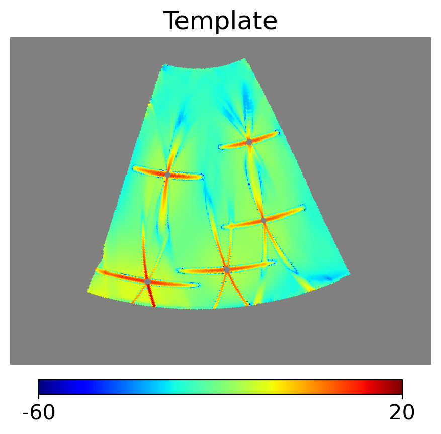
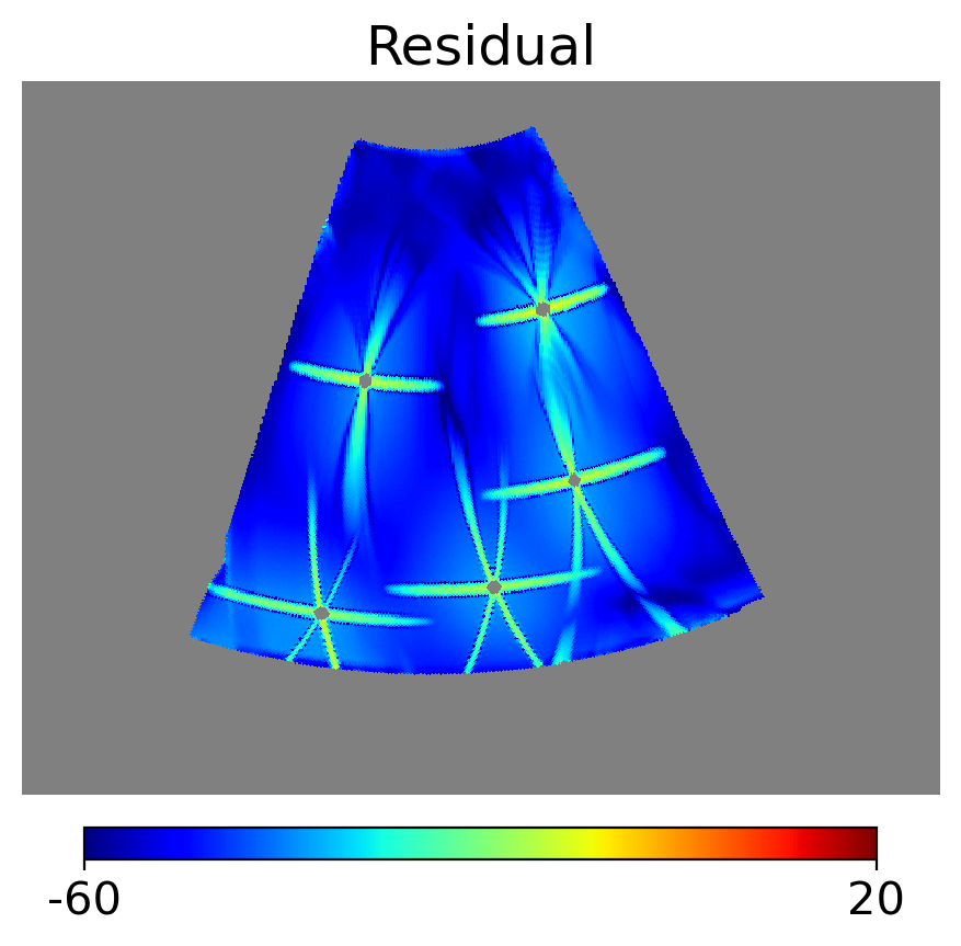
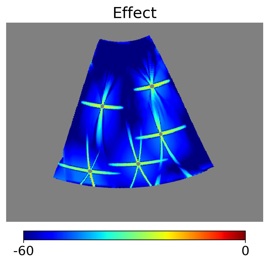
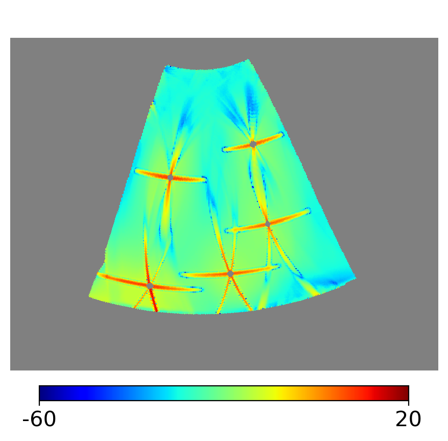
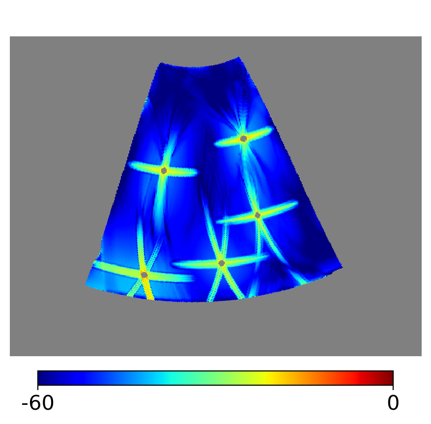
Figure 3: Same as in Fig. 1, but for the case of multiple point sources with unknown polarization direction, where the residuals are estimated through Eq. 3.2.

As shown in Fig. 4, using a logarithmic scale, we also compute the angular power spectrum of CMB, residuals, and true leakage for multiple point sources with unknown polarization directions. When compared to the spectrum of two templates, the spectrum of two residuals is 2 to 3 orders of magnitudes smaller. Our method can improve the performance of the probe since the $BB$ spectrum of residual is substantially smaller after our correction method than that of CMB. In addition, there are some fluctuations of the $BB$ power spectrum for CMB in small multipole $\ell$ as we only study a portion of sky map. Furthermore, the power spectrum with unknown polarization direction is also a little greater than that with known polarization direction. This is because two fitting parameters can introduce more errors, which causes the residual to increase.

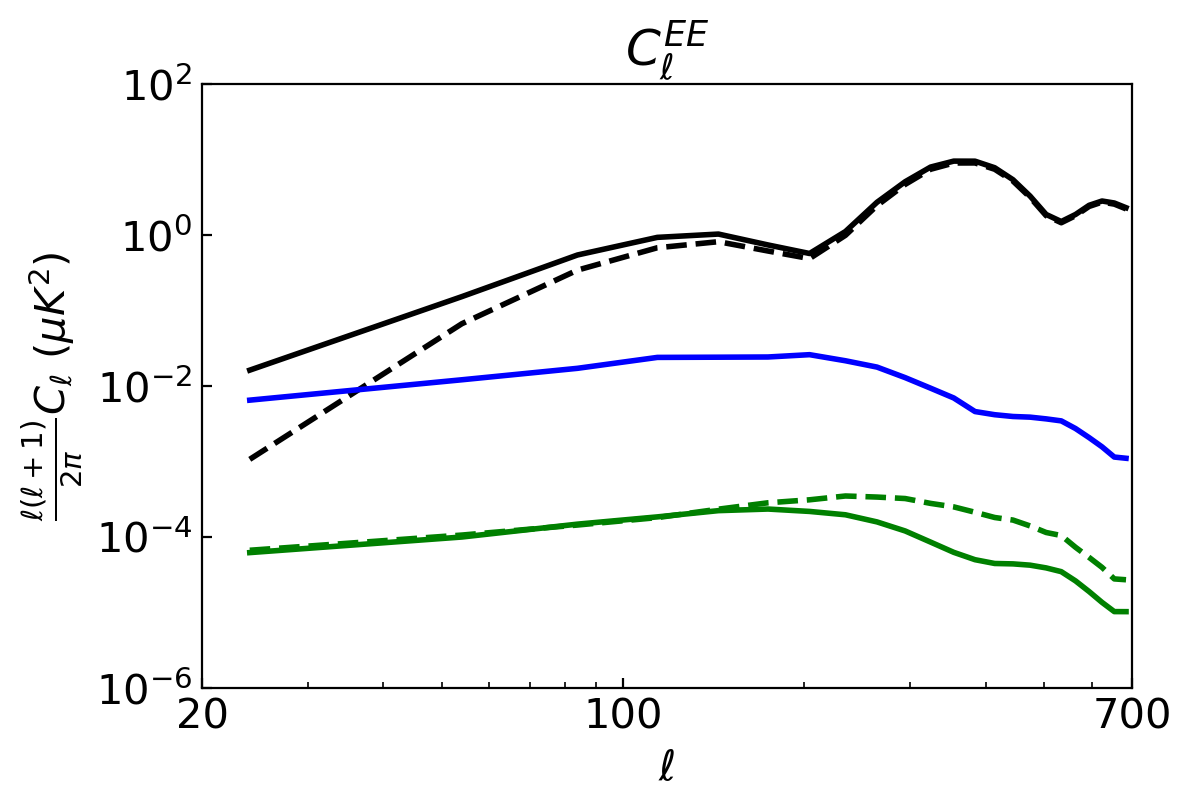
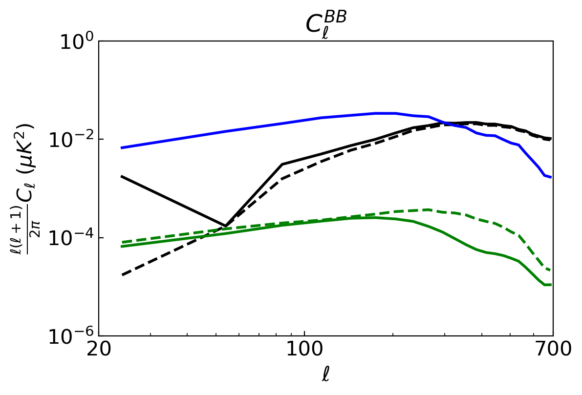
Figure 4: Same as in Fig. 2, but for the case of multiple point sources with unknown polarization direction.

In conclusion, even when the number of point sources rises, our correction method maintains good accuracy and reliability. Regardless of whether there are one or more point sources, fitting parameters are almost identical. The amplitude of residuals after correction is much lower than that of the template in the pixel domain. After correction, the residual spectrum is considerably smaller than the CMB spectrum, thus the impact of point source leakage is significantly reduced by our method.

3.3 Actual point sources

To simulate the actual sky map, we use the data from 2013 Planck Catalogue of Compact Sources(PCCS). In the region we study (the same region as in Fig. 3), the flux data of the 10 brightest point sources at 100 GHz are used to calculate the conversion coefficient from flux to temperature, which is equal to 2.879 $\mu$K$\cdot\mathrm{mJy}^{-1}$. The approximate temperature of these 10 brightest point sources is then determined. The point source polarization is assumed to be roughly 40 percent of its temperature. Since the precise point source polarization directions are unknown before we get the corrected map, a certain polarization direction is specified for each point source to construct two types of templates for simplification of calculation. According to the fitting parameter results in Tab. 4, for both the ideal and realistic templates, the ratio of fitting parameters $k^{U}/k^{Q}$ for each point source is close to $\tan(2\theta)$.

Table 4: Location, temperature, polarization and fitting parameter result with random polarization direction of actual 10 brightest point sources in the region we study (the region shape is the same with Fig. 3).

Number	$[b,l]^{\circ}$	$I/\mu$K	$P/\mu$K	$\theta^{\circ}$	$k_{0}^{Q}$	$k_{1}^{Q}$	$k_{0}^{U}$	$k_{1}^{U}$	$k_{0}^{U}/k_{0}^{Q}$	$k_{1}^{U}/k_{1}^{Q}$	$\tan(2\theta)$
1	[46.2, 183.7]	880.4	352.1	155.8	0.939	-1.039	1.119	-1.237	-1.107	-1.106	-1.125
2	[31.9, 200.0]	378.2	151.3	25.0	0.927	1.074	1.098	1.271	1.159	1.157	1.191
3	[44.8, 175.7]	331.0	132.4	25.8	0.914	1.100	1.084	1.306	1.203	1.205	1.258
4	[58.5, 177.6]	232.3	92.9	20.1	1.124	0.785	1.433	0.999	0.698	0.697	0.844
5	[22.8, 196.5]	186.0	74.4	153.3	0.774	-1.096	1.042	-1.516	-1.416	-1.455	-1.351
6	[33.3, 178.2]	185.9	74.4	103.3	-1.225	-0.678	-1.430	-0.784	0.553	0.548	0.500
7	[46.8, 167.3]	162.4	64.9	171.4	1.348	-0.467	1.596	-0.565	-0.347	-0.354	-0.311
8	[44.6, 198.8]	159.6	63.8	28.4	0.846	1.147	1.038	1.393	1.356	1.342	1.530
9	[49.1, 147.7]	145.8	58.3	17.9	1.136	0.711	1.381	0.876	0.626	0.634	0.724
10	[69.8, 174.7]	139.5	55.8	112.5	-1.040	-0.922	-1.540	-1.376	0.887	0.893	0.999

We again build the sky map showing the polarization dB value of the templates, residuals and dB effects for actual point sources (Fig. 5). The results are similar to Fig. 3, as detailed in Tab. 5.

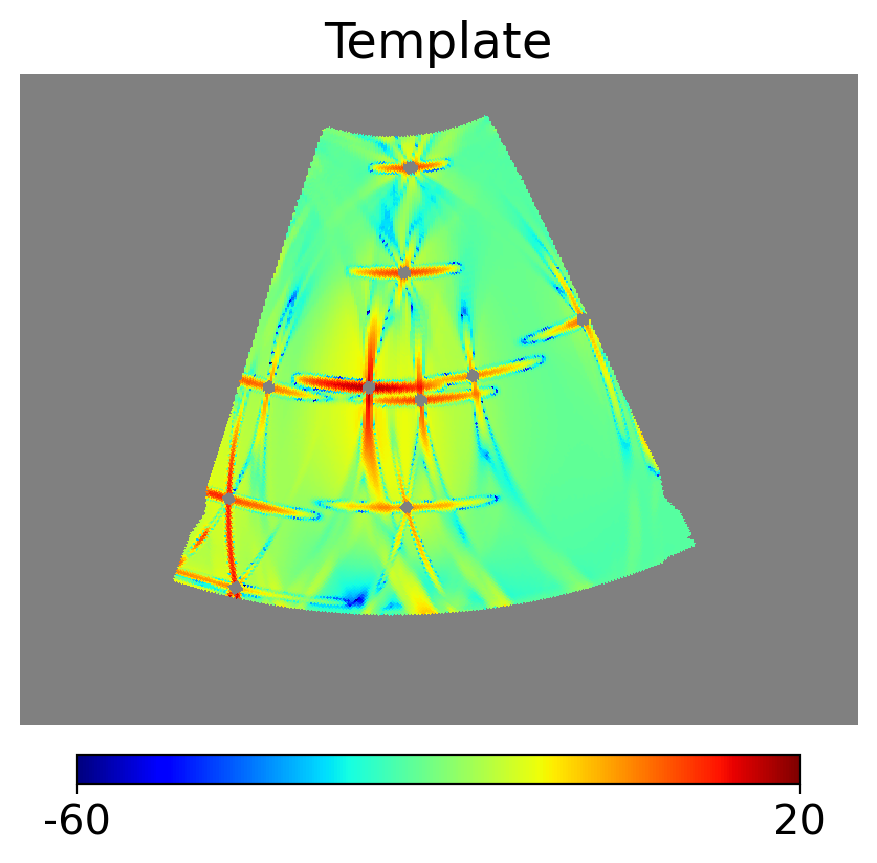
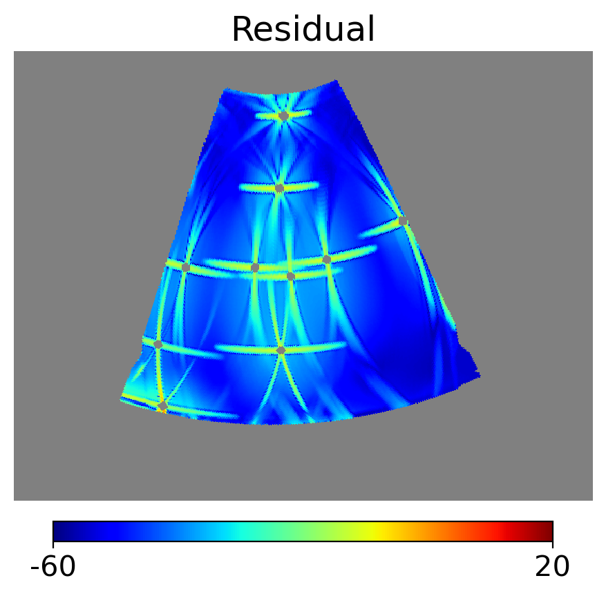
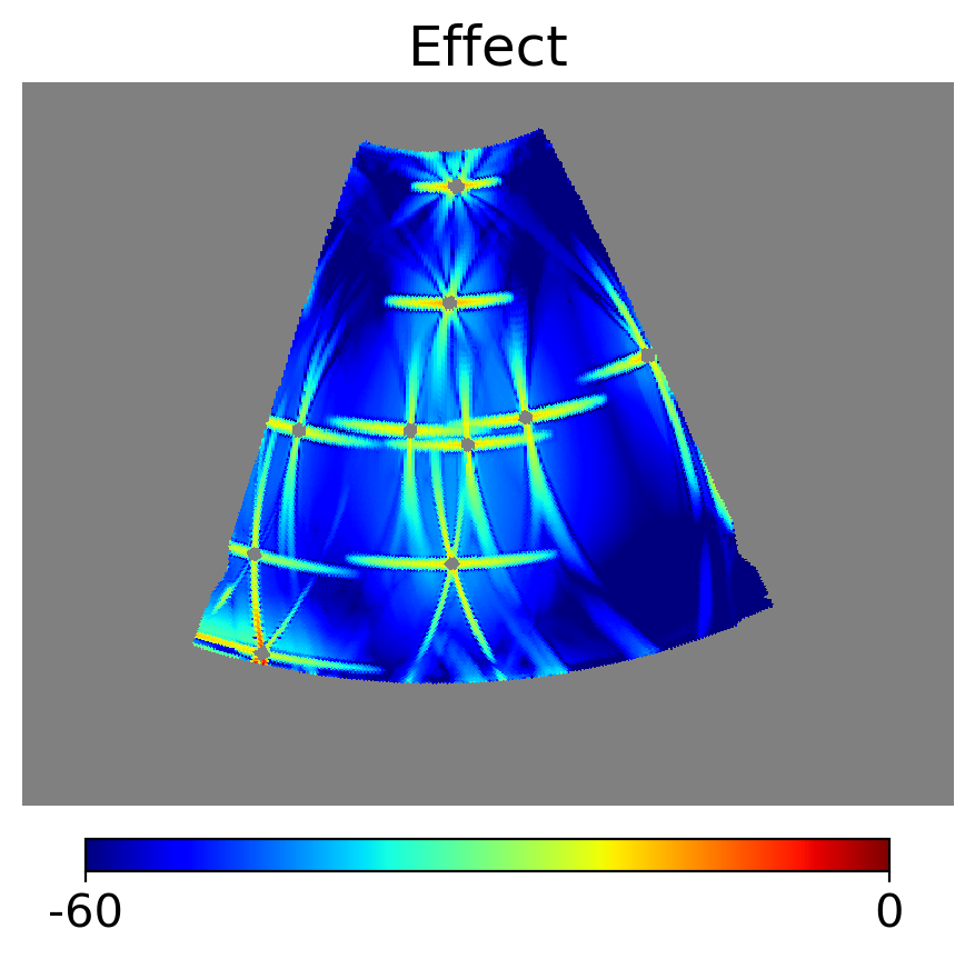
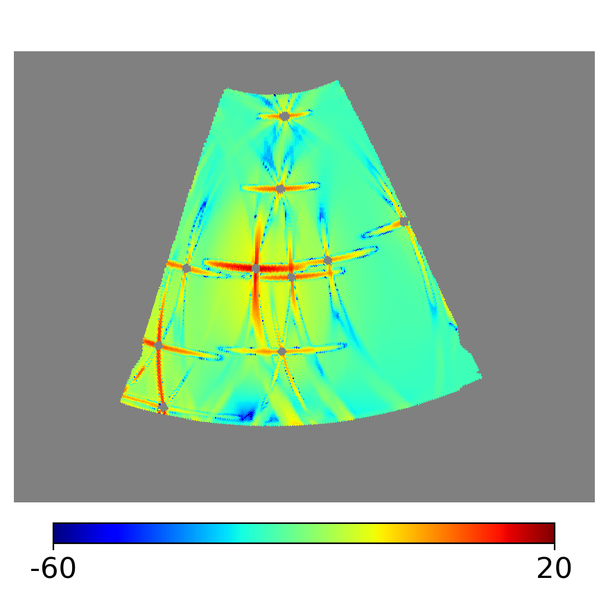
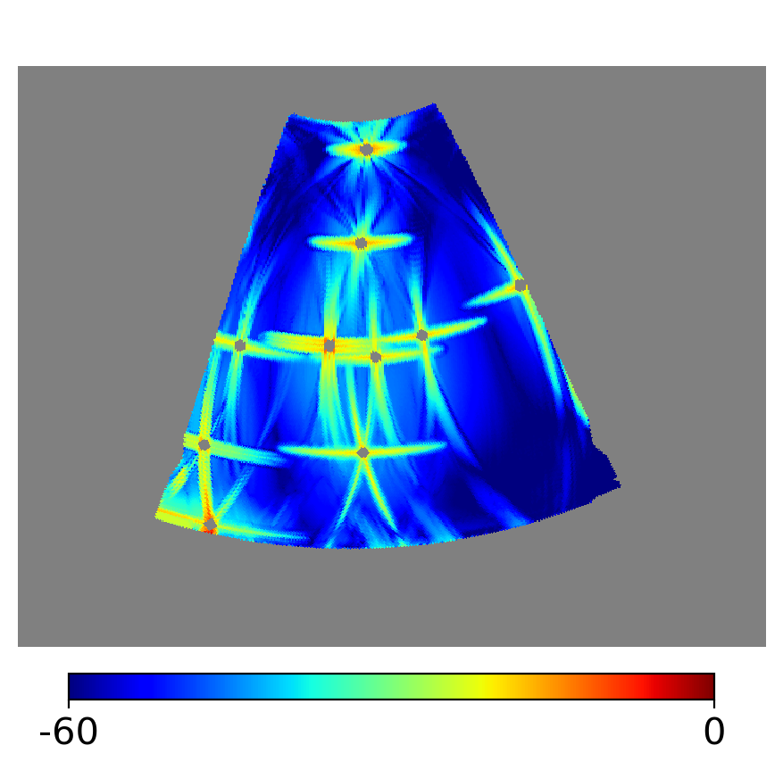
Figure 5: Same as in Fig. 1, but for the case of actual point sources with unknown polarization direction, where the residuals are estimated using Eq. 3.2.

Table 5: Comparison of the standard deviation of $\sigma_{*}=10^{-2}$ $\mu\rm K$ of filtered CMB, foreground, noise, and actual 10 brightest point sources simulation residuals with unknown polarization direction in the pixel domain.

$\sigma_{d^{\prime}_{c}}/\sigma_{*}$	$\sigma_{d^{\prime}_{f}}/\sigma_{*}$	$\sigma_{n^{\prime}}/\sigma_{*}$	$\sigma_{\delta_{0}}/\sigma_{*}$	$\sigma_{\delta_{1}}/\sigma_{*}$
49.826	3.455	15.439	0.881	1.093

In Fig. 6, with our correction method, the angular power spectrum of residual is again substantially smaller than that of the true leakage and the expected CMB signal, demonstrating the effectiveness of our method with realistic point sources.

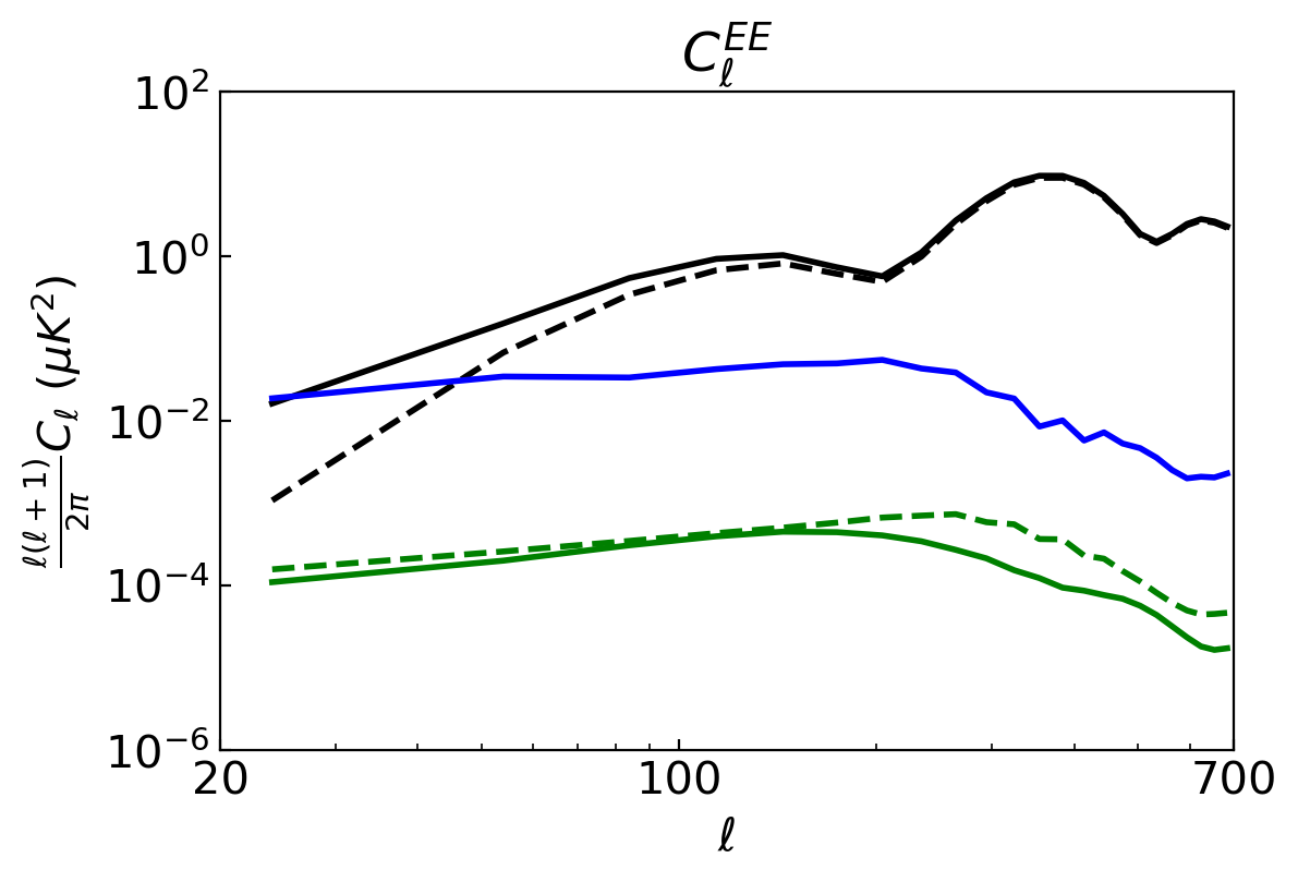
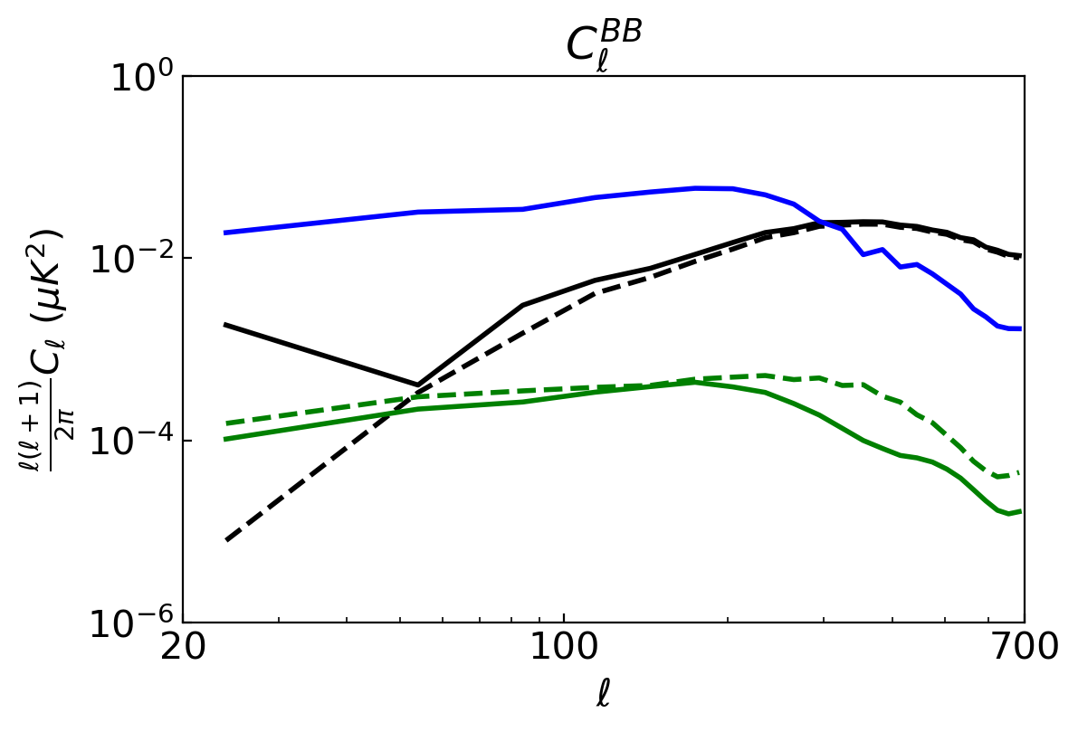
Figure 6: Same as in Fig. 2, but for the case of the actual point sources with unknown polarization directions.

4 Discussion

In this work, we have introduced a novel ”template-fitting” method (Sect. 2) for removing the point source leakage due to time-order data filtering. The key ingredient of this method is to construct several templates of the leakage for each point source in pixel domain and then to remove this leakage contamination by fitting these templates. Several tests for single, multi and realistic point source simulations (Sect. 3) are present to demonstrate the effectiveness of our method. The leakage after template fitting is typically star-like, and can be reduced by 1-2 orders of magnitude in the pixel domain and by 3-4 orders of magnitude in angular power spectrum. The performance of our method is robust in all simulations. According to the calculation of the angular power spectrum of the residuals (see Figs. 2, 4, 6), we can see that the residual $BB$ spectrum is about two orders of magnitudes lower than the theoretical prediction for the primordial gravitational waves with $r\sim 10^{-2}$. Therefore, our method can easily satisfy the detection requirement for small $r$ down to $r\sim 10^{-3}$.

Using the matrix-based pipeline, the application of our template fitting method in this study becomes very practical. However, it is preferable to utilize a conventional non-matrix pipeline to execute our approach, which is because the construction of a full matrix for high-resolution map is impossible (scaled as $N^{2}_{\rm pix}$), due to the limitations in memory and storage. Fortunately, the standard non-matrix pipeline can be used with our method as well, as mentioned in Sect. 2.2. In brief, all that needs to be done is to mask the map created by the standard pipeline with a point source mask, and then feed the masked sky map back into the pipeline to obtain the realistic templates. This fact allows our method to be functional even at high resolution, which is very useful in practice.

References

- [1] B. G. Keating, P. A. R. Ade, J. J. Bock, E. Hivon, W. L. Holzapfel, A. E. Lange et al., BICEP: a large angular scale CMB polarimeter, in Polarimetry in Astronomy (S. Fineschi, ed.), vol. 4843 of Society of Photo-Optical Instrumentation Engineers (SPIE) Conference Series, pp. 284–295, Feb., 2003, DOI.
- [2] The Planck Collaboration, The Scientific Programme of Planck, arXiv e-prints (Apr., 2006) astro–ph/0604069, [astro-ph/0604069].
- [3] J. A. Rubiño-Martín, R. Rebolo, M. Tucci, R. Génova-Santos, S. R. Hildebrandt, R. Hoyland et al., The QUIJOTE CMB Experiment, in Highlights of Spanish Astrophysics V, vol. 14 of Astrophysics and Space Science Proceedings, p. 127, Jan., 2010, 0810.3141, DOI.
- [4] M. D. Niemack, P. A. R. Ade, J. Aguirre, F. Barrientos, J. A. Beall, J. R. Bond et al., ACTPol: a polarization-sensitive receiver for the Atacama Cosmology Telescope, in Millimeter, Submillimeter, and Far-Infrared Detectors and Instrumentation for Astronomy V (W. S. Holland and J. Zmuidzinas, eds.), vol. 7741 of Society of Photo-Optical Instrumentation Engineers (SPIE) Conference Series, p. 77411S, July, 2010, 1006.5049, DOI.
- [5] J. E. Austermann, K. A. Aird, J. A. Beall, D. Becker, A. Bender, B. A. Benson et al., SPTpol: an instrument for CMB polarization measurements with the South Pole Telescope, in Millimeter, Submillimeter, and Far-Infrared Detectors and Instrumentation for Astronomy VI (W. S. Holland and J. Zmuidzinas, eds.), vol. 8452 of Society of Photo-Optical Instrumentation Engineers (SPIE) Conference Series, p. 84521E, Sept., 2012, 1210.4970, DOI.
- [6] G. Hinshaw, D. Larson, E. Komatsu, D. N. Spergel, C. L. Bennett, J. Dunkley et al., Nine-year Wilkinson Microwave Anisotropy Probe (WMAP) Observations: Cosmological Parameter Results, Astrophys. J.Suppl. 208 (Oct., 2013) 19, [1212.5226].
- [7] Planck Collaboration, N. Aghanim, Y. Akrami, M. Ashdown, J. Aumont, C. Baccigalupi et al., Planck 2018 results. VI. Cosmological parameters, arXiv e-prints (Jul, 2018) arXiv:1807.06209, [1807.06209].
- [8] BICEP2/Keck Collaboration, Planck Collaboration, P. A. R. Ade, N. Aghanim, Z. Ahmed, R. W. Aikin et al., Joint Analysis of BICEP2/Keck Array and Planck Data, Physical Review Letters 114 (Mar., 2015) 101301, [1502.00612].
- [9] BICEP2 Collaboration, Keck Array Collaboration, P. A. R. Ade, Z. Ahmed, R. W. Aikin, K. D. Alexand er et al., Constraints on Primordial Gravitational Waves Using Planck, WMAP, and New BICEP2/Keck Observations through the 2015 Season, Phys. Rev. Lett. 121 (Nov., 2018) 221301, [1810.05216].
- [10] BICEP/Keck Collaboration collaboration, P. A. R. Ade, Z. Ahmed, M. Amiri, D. Barkats, R. B. Thakur, C. A. Bischoff et al., Improved constraints on primordial gravitational waves using planck, wmap, and bicep/keck observations through the 2018 observing season, Phys. Rev. Lett. 127 (Oct, 2021) 151301.
- [11] B. Keating, S. Moyerman, D. Boettger, J. Edwards, G. Fuller, F. Matsuda et al., Ultra High Energy Cosmology with POLARBEAR, ArXiv e-prints (Oct., 2011) , [1110.2101].
- [12] M. Hazumi, J. Borrill, Y. Chinone, M. A. Dobbs, H. Fuke, A. Ghribi et al., LiteBIRD: a small satellite for the study of B-mode polarization and inflation from cosmic background radiation detection, in Space Telescopes and Instrumentation 2012: Optical, Infrared, and Millimeter Wave, vol. 8442 of Proc. SPIE, p. 844219, Sept., 2012, DOI.
- [13] K. N. Abazajian, P. Adshead, Z. Ahmed, S. W. Allen, D. Alonso, K. S. Arnold et al., CMB-S4 Science Book, First Edition, ArXiv e-prints (Oct., 2016) , [1610.02743].
- [14] P. Ade, J. Aguirre, Z. Ahmed, S. Aiola, A. Ali, D. Alonso et al., The Simons Observatory: science goals and forecasts, JCAP 2019 (Feb., 2019) 056, [1808.07445].
- [15] H. Li, S.-Y. Li, Y. Liu, Y.-P. Li, Y. Cai, M. Li et al., Probing primordial gravitational waves: Ali CMB Polarization Telescope, National Science Review 6 (02, 2018) 145–154, [http://oup.prod.sis.lan/nsr/article-pdf/6/1/145/27981397/nwy019.pdf].
- [16] H. Liu, J. Creswell, S. von Hausegger and P. Naselsky, Methods for pixel domain correction of E B leakage, Phys. Rev. D 100 (Jul, 2019) 023538, [1811.04691].
- [17] S. Ghosh et al., Performance forecasts for the primordial gravitational wave detection pipelines for AliCPT-1, 2205.14804.
- [18] H. Li et al., Probing Primordial Gravitational Waves: Ali CMB Polarization Telescope, Natl. Sci. Rev. 6 (2019) 145–154, [1710.03047].
- [19] M. Salatino, J. Austermann, K. L. Thompson, P. Ade, X. Bai, J. Beall et al., The design of the ali CMB polarization telescope receiver, in Millimeter, Submillimeter, and Far-Infrared Detectors and Instrumentation for Astronomy X (J. Zmuidzinas and J.-R. Gao, eds.), SPIE, dec, 2020, DOI.
- [20] Planck Collaboration, P. A. R. Ade, N. Aghanim, C. Armitage-Caplan, M. Arnaud, M. Ashdown et al., Planck 2013 results. IX. HFI spectral response, Astr. Astrophys. 571 (Nov., 2014) A9, [1303.5070].