Can Knowledge of End-to-End Text-to-Speech Models Improve Neural MIDI-to-Audio Synthesis Systems?

Abstract

With the similarity between music and speech synthesis from symbolic input and the rapid development of text-to-speech (TTS) techniques, it is worthwhile to explore ways to improve the MIDI-to-audio performance by borrowing from TTS techniques. In this study, we analyze the shortcomings of a TTS-based MIDI-to-audio system and improve it in terms of feature computation, model selection, and training strategy, aiming to synthesize highly natural-sounding audio. Moreover, we conducted an extensive model evaluation through listening tests, pitch measurement, and spectrogram analysis. This work demonstrates not only synthesis of highly natural music but offers a thorough analytical approach and useful outcomes for the community. Our code, pre-trained models, supplementary materials, and audio samples are open sourced at https://github.com/nii-yamagishilab/midi-to-audio .

Index Terms—  music audio synthesis, text to speech synthesis, deep learning, Tacotron, Transformer, neural vocoder

1 Introduction

Generating musical instrument sounds using data-driven neural synthesis approaches allows us to benefit from advances in sequence-to-sequence modeling [1, 2], to learn from audio examples [3, 4], and to flexibly interpolate and transform instrument sounds [5, 6]. Compared with sample-based synthesis such as Fluidsynth [7] and physical modeling based approaches such as Pianoteq [8], data-driven neural MIDI-to-audio synthesis allows us to flexibly generate new instrument sounds without having to painstakingly specify the physical parameters of every instrument by hand.

Although there are differences between musical instrument sounds and speech sounds, we showed in our past work [1] that text-to-speech synthesis architectures composed of an acoustic model and a neural vocoder can be modified for the task of generating piano sounds from MIDI input. This opens up many possibilities for musical sound generation that conceptually match well with tasks in speech generation, such as musical style transfer using style tokens [9, 10], multi-instrument modeling in the manner of multi-language multi-speaker TTS [11, 12], and timbre transfer and interpolation based on voice conversion frameworks [5, 13].

However, while speech synthesis has reached a level of quality where it can be almost indistinguishable from human speech, we still observe a gap in quality between our synthesized audio and real piano sounds. In this paper, we address this quality gap with several proposed improvements, and we analyze our synthesized audio to identify further areas for improvement.

The first of our proposed improvements is joint training of the acoustic model and neural vocoder. In TTS, the acoustic model and neural vocoder are often separately trained, but it is also known that this results in degraded sound quality [14, 15] since separate training may cause a mismatch due to the fact that the neural vocoder is trained using natural spectrograms, whereas generated spectrograms are input at inference time. We hypothesize that the joint training of the two models will improve the quality of the generated audio even for the case of musical instrument sounds. Second, we introduce improved acoustic model and vocoder architectures in terms of training efficiency. In our prior work we used a Tacotron 2 [14] architecture with a neural source-filter (NSF) [16] vocoder, and in this work, we explore the Transformer TTS architecture [17] as well as the HiFiGAN vocoder [18] and its combination with NSF. Finally, our prior work used the MIDI-scale spectrogram instead of the Mel spectrogram, but the number of fast Fourier transform (FFT) points was not big enough to perfectly support a MIDI-scale filter bank. We fix this issue by using a larger number of FFT points.

We evaluated our proposed improvements in a crowdsourced mean opinion score (MOS) listening test, which revealed that the improved system using the above refinements can lead to high-fidelity waveform signals and produce a higher quality of audio than the standard MIDI player. However, the results also show that there is still a gap between natural and generated audio. We further analyzed the objective and subjective results at the note level and identified areas for further improvement.

This paper is structured as follows: Section 2 reviews related work on MIDI-to-audio synthesis, and the proposed improvements are described in Section 3. Section 4 describes the experiments, and our findings are summarized in Section 5.

2 Background

Several deep learning-based algorithms have been proposed to generate music from musical notes. PerformanceNet [3] uses a U-Net-based ContourNet and a multi-band residual network-based TextureNet to transfer piano roll input to a spectrogram. It then uses the Griffin-Lim algorithm [19] to reconstruct a waveform. Derived from DDSP [13], MIDI-DDSP [6] integrates three separately trained modules in a hierarchical way to control the notes, performance, and synthesis factors, respectively. MIDI-DDSP is capable of synthesizing high-fidelity audio while keeping interactive control of the synthesis. Deep Performer [2] explicitly models necessary factors for audio synthesis with individual models and uses a Transformer to generate a Mel-spectrogram. It then uses a separately trained HiFi-GAN to transform the Mel-spectrogram into music audio. Our previous work [1] observed a similarity between TTS and MIDI-to-audio synthesis and used a Tacotron-based acoustic model and an NSF-based waveform model to synthesize audio from aligned piano roll input.

3 MIDI-to-audio synthesis system based on TTS techniques and its improvements

3.1 Overview of baseline MIDI-to-audio synthesis system

The MIDI-to-audio synthesis process is similar to TTS in the sense that both convert symbolic data into audio signals.

The input MIDI contains messages that encode the note identity, the time of note onset and offset, velocity, and other events. For processing using deep learning models, MIDI input is often represented as a piano roll, which is a sequence of multi-hot vectors, where each multi-hot vector is 128 dimensions. Each dimension encodes the velocity for one of the 128 MIDI notes.

Using a sequence of multi-hot vectors as an input, a sequence-to-sequence model transforms it into a sequence of acoustic features that are suitable to drive a neural waveform model. In our previous work [1], we used a variant of Tacotron 2 with self-attention as the acoustic model [20] and a 128-dimensional MIDI-scaled spectrogram [1], which is similar to the Mel spectrogram but uses a filter-bank located at the center frequencies of MIDI notes. As for the neural waveform model, we used NSF[16].

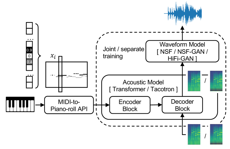
Fig. 1: Architecture of investigated methods.

3.2 Shortcomings of baseline and proposed refinements

Our previous study showed that the generated audio samples from the baseline system with the best configuration achieved an acceptable MOS of around 3.2 [1], but it was significantly lower than the score of 4.0 obtained for the natural audio. One major factor we identified is the feature mismatch for the input to the neural vocoder. While the neural vocoder was trained with acoustic features extracted from natural audio as input, it took as input the acoustic features generated by the acoustic model during inference.

A similar issue had raised concerns in the TTS community and inspired a few methods for refinement. We are motivated to analyze how well these methods can be applied to the MIDI-to-audio sound generation task. The first improvement is joint training of the acoustic model and neural vocoder. This is done by concatenating the two models, conducting back-propagation from the generated audio waveform to the input MIDI sequence, and jointly optimizing both modules. By doing so, the neural vocoder takes the acoustic model’s output as input both in the training and inference stage, which alleviates the feature mismatch.

Since the two modules affect the performance of the whole system, the second refinement is to explore better architectures for each of them. In this study, we investigate the Transformer TTS architecture and the HiFi-GAN (and its combination with NSF) as improved acoustic model and neural vocoders, respectively. The reason to investigate Transformer is its superior performance in speech synthesis [17] and other audio processing tasks [21]. As for waveform models, NSF, which uses only a multi-resolution short-time Fourier transform (STFT) loss [16], suffers from the limitations of a maximum-likelihood-based model training criterion. We expect that GAN-based waveform models such as HiFi-GAN can further improve the system performance. Meanwhile, we can combine the NSF model and the HiFi-GAN discriminators to address the limitations of NSF. We refer to this model as NSF-GAN.

Another refinement is on the acoustic features. The original implementation of the MIDI spectrogram uses only a 4,096-point FFT, but the width of the first few filters in the MIDI filter-bank is narrower than 2 Hz and may not cover any FFT frequency bin. Hence, as shown in the Fig.4 of [1], these filter outputs, or the corresponding feature dimensions of the MIDI spectrogram, become zero. As refinement, we increase the number of FFT points by a factor of four to 16,384 when extracting the MIDI-spectrogram.

4 Experiments

4.1 Experimental condition

Database: We used the MAESTRO dataset [22] to explore piano audio synthesis. MAESTRO was collected from the international Piano-e-Competition. In addition to the concert-quality piano performances presented by virtuoso pianists, a high-precision sensor built into the piano captures the time-aligned MIDI transcription of each performance with an accuracy of 3 ms. The MAESTRO dataset has 1,276 performances totaling 198.7 hours, which were divided into training, validation, and test sets with 962, 137, and 177 performances totaling respectively 159.2, 19.4, and 20.0 hours.

In our experiments, we followed the split configuration in [22] but resampled the audio to 24 kHz. We further preprocessed the data in two ways to accommodate the synthesis system. First, we segmented each long sample into short pieces of 800 frames for training to avoid memory issues; second, we converted the MIDI input, which uses an onset/offset representation of notes, into a piano roll format to make it simpler for the model to parse the notes. We used the PrettyMIDI API [23] to convert MIDI files into piano rolls.

Systems: Experimental models are listed in the left-most column of Table 1. Following [1], we included the sample-based synthesizer Fluidsynth and the physical model synthesizer Pianoteq as reference. Other systems followed the same framework in Figure 1 but varied in the choice of the acoustic model, acoustic features, waveform model, and training strategy. Only abs-mfbf-nsfs and taco-mfbf-nsfs used the inadequate MIDI spectrogram [1], while others used the refined version. Systems with the ID abs are analysis-by-synthesis systems that used the acoustic features of natural audio as input to the waveform model. They were included to measure the waveform models’ performances.

The investigated acoustic models included Transformer TTS [17] using an implementation from ESPnet [24], and a variant of Tacotron [25] using an implementation from [20]. Following [1], we set the dropout rate of the postnet to 0.99 to alleviate the issue of exposure bias [26]. We also set the reduction factor to $4$ and fixed the length of input to $800$ frames. For waveform models, we compared NSF (nsf) [16], HiFi-GAN (hfg) [18], and NSF-GAN (nsfg), all of which were implemented on ESPNet. NSF used the same configuration as that in [1], HiFi-GAN used the default configuration set by ESPNet, and NSF-GAN combined the two. For a sanity check and fair comparison with [1], we used the original NSF implementation, which is not implemented in ESPnet. This waveform model is denoted as nsfs.

The experimental systems were trained using either a separate-training or a joint-training strategy. In the former case, the acoustic and waveform models were trained separately. The Transformer acoustic model was trained using the Adam optimizer [27] with a learning rate of $1$ for 200k steps, while the training strategy of Tacotron followed [1]. The waveform models were trained using the AdamW optimizer with a learning rate of $2\times 10^{-4}$ for one million training steps. For the joint-training strategy, each component was first trained using the same configuration as in the separate-training strategy, after which they were jointly fine-tuned with the Adam optimizer and a learning rate of $1.25\times 10^{-5}$ for 200k steps.

4.2 Subjective evaluation

Table 1: Experimental systems and evaluation results.

System ID	Acoustic model	Acoustic feature	Wave. model	Joint train	Obj. Eval.			MOS (mean)
					Pitch	Chroma	Spec.
Natural	-	-	-	-	-	-	-	3.98
Software-based baselines
Fluidsynth	Sample-based MIDI-to-audio s.w.				1.00	0.33	13.95	3.56
Pianoteq	Physical-model MIDI-to-audio s.w.				0.92	0.32	12.16	4.10
Synthesis system trained on flawed MIDI spectrogram
abs-mfbf-nsfs	-	midi-fb-f	NSF[1]	-	1.01	0.31	6.60	3.71
taco-mfbf-nsfs	taco	midi-fb-f	NSF[1]	-	1.18	0.37	9.65	2.95
Waveform model trained on refined MIDI spectrogram
abs-mfb-nsfs	-	midi-fb	NSF[1]	-	1.31	0.38	5.72	3.31
abs-mfb-nsf	-	midi-fb	NSF	-	1.37	0.39	7.20	3.35
abs-mfb-nsfg	-	midi-fb	NSF-GAN	-	1.26	0.34	5.14	3.69
abs-mfb-hfg	-	midi-fb	HiFi-GAN	-	1.16	0.31	4.69	3.80
Acoustic model trained on refined MIDI spectrogram
taco-mfb-nsfs	taco	midi-fb	NSF[1]	-	1.19	0.37	9.70	3.16
taco-mfb-nsf	taco	midi-fb	NSF	-	1.29	0.40	11.78	3.16
taco-mfb-nsfg	taco	midi-fb	NSF-GAN	-	1.11	0.35	9.09	3.18
taco-mfb-hfg	taco	midi-fb	HiFi-GAN	-	1.58	0.56	10.07	2.21
trans-mfb-nsfs	trans	midi-fb	NSF[1]	-	1.33	0.41	9.41	3.22
trans-mfb-nsf	trans	midi-fb	NSF	-	1.42	0.44	10.94	3.10
trans-mfb-nsfg	trans	midi-fb	NSF-GAN	-	1.27	0.40	9.15	3.08
trans-mfb-hfg	trans	midi-fb	HiFi-GAN	-	1.83	0.60	9.95	1.88
Joint training of acoustic and waveform model
joint-nsf	trans	midi-fb	NSF	✓	1.59	0.47	16.39	2.23
joint-nsfg	trans	midi-fb	NSF-GAN	✓	1.12	0.38	9.09	3.32
joint-hfg	trans	midi-fb	HiFi-GAN	✓	1.10	0.38	9.14	3.58

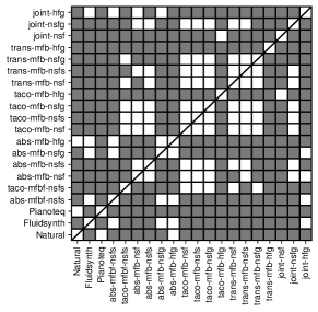
Fig. 2: Results of two-sided Mann-Whitney U test with Holm-Bonferroni correction. Grey block indicates statistically significant difference at $\alpha=0.05$

An extensive crowdsourced subjective listening test was conducted to evaluate the quality of the natural and synthesized audio from all the experimental systems. We split the audio samples on the basis of the locations of long pauses into segments that lasted from around 10 to 30 seconds. We then randomly selected 102 segment IDs and picked up corresponding segments from each systems as the listening test samples. Each listening test set had 30 different samples, balanced to contain at least one sample from each of the experimental systems. Listeners were instructed to rate the overall quality of each sample using a scale from 1 (very bad) to 5 (very good), and they were allowed to rate at most 10 different sets. In total, there were 229 listeners, leading to 340 valid sets of results, and Table 1 shows MOS. We also conducted a statistical analysis using the two-sided Mann-Whitney U test with Holm-Bonferroni correction, the results of which are shown in Figure 2. The results allowed us to assess the effectiveness of the proposed refinements.

Did advanced acoustic and waveform models help? In the analysis-by-synthesis condition, the HiFi-GAN waveform model abs-mfb-hfg achieved a MOS of 3.80, which outperformed the NSF models abs-mfb-nsfs and abs-mfb-nsf with a statistically significant difference ($p\ll{1\mathrm{e}-10}$). Furthermore, abs-mfb-hfg was not statistically different from the natural recordings and the sample-based synthesizer Fluidsynth. Using a GAN-based waveform model may be essential. In fact, by simply combining the HiFi-GAN’s discriminators with NSF, the resulting NSF-GAN abs-mfb-nsfg also outperformed the two original NSF models with a statistically significant margin.

However, the gains brought by HiFi-GAN diminished when the acoustic features were predicted from separately trained acoustic models. Systems taco-mfb-hfg and trans-mfb-hfg, which used a HiFi-GAN waveform model, were significantly worse than the other systems using NSF-based models. We argue that the reason is because the non-linear transformation in HiFi-GAN is sensitive to shifted parameters, while residual networks in NSF are able to encode correct synthesis parameters from distorted input.

The acoustic models did not show a significant difference in MOS when combined with a separately trained NSF-based acoustic model (taco-mfb-nsf* compared with each respective trans-mfb-nsf*).

Did joint-training strategy improve system performance? The results from the last six rows of Table 1 showed that the joint-training strategy significantly improved the system performance if the system used a GAN-based waveform model. Particularly, joint-hfg, which jointly optimized the Transformer and HiFi-GAN, achieved a MOS of 3.58, which was significantly higher than the counterpart trans-mfb-hfg using a separate-training strategy ($p\ll{1\mathrm{e}-100}$). A similar improvement can be observed from the comparison between joint-nsfg and trans-mfb-nsfg.

Figure 3 illustrates a Rainbow-gram of natural and generated audio from trans-mfb-hfg and joint-hfg. From the natural audio’s sub-figure, we can easily observe the notes and harmonics. In trans-mfb-hfg, the harmonics, especially in the high-frequency band, are less clear, and there was higher energy between harmonics. Furthermore, the low-frequency band has artifacts (e.g., horizontal bars) at the beginning of silence. Such degradation and artifacts were alleviated in the case of joint-hfg.

When using NSF, the joint-training strategy harmed joint-nsf. One possible reason is that NSF is limited by maximum-likelihood-based STFT loss and lacks the capacity to produce high-quality waveforms from hidden acoustic features in a jointly trained system. Adding adversarial loss can help, and this suggests again the advantage of using a GAN-based waveform model.

Overall performance: By combining the best components and training strategy, joint-hfg outperformed other MIDI-to-audio synthesis systems with statistically significant differences, including the system proposed in our previous work. Note that the refined MIDI spectrogram also contributed because the comparison between taco-mfbf-nsfs and taco-mfb-nsfs showed that the refined MIDI spectrogram was beneficial. However, the MOS of joint-hfg was still lower than those of natural audio. This quality gap calls for further investigation, and part of it is presented in the objective analysis in the next section.

The physical-model-based Pianoteq outperformed even the natural audio (although not statistically significantly), a finding consistent with previous work [1]. However, the physical model is the outcome of laborious analysis and simulation, which does not easily generalize to other types of piano or different instruments.

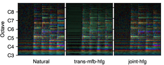
Fig. 3: Rainbow-gram of Natural and HiFi-GAN-based systems.

4.3 Analysis with objective metrics

We measured a few distance metrics between the synthesized and natural audio, including the pitch, Chroma, and MIDI spectrogram distortion. The last two were computed using mean squared error (MSE). The 12-dimensional Chroma features were extracted using librosa [28]. The pitch distortion was the cross-entropy between the estimated pitch probabilities of the synthesized and natural audio [1]. The pitch estimation was done using CREPE [29].

Results are listed in Table 1. We computed the correlation of these objective results with MOS. We found that both pitch and Chroma distortion had a negative correlation with MOS at $-0.88$ and $-0.91$, which indicates that the listeners were sensitive to out-of-tune notes. The MIDI spectrogram distortion also showed a negative correlation with MOS on data-driven systems at $-0.68$.

On the basis of the above utterance-level analysis, we further analyzed how objective metrics correlate with the MOS at the note level. Given the MOS ratings for synthesized audio samples from one system, we (approximately) computed an averaged MOS for each note that appeared. Since each dimension of the MIDI spectrogram corresponds to one note, the MIDI spectrogram distortion for each note was computed over the corresponding feature dimension. The note-level pitch distortion was computed using CREPE and cross-entropy without averaging over the notes.

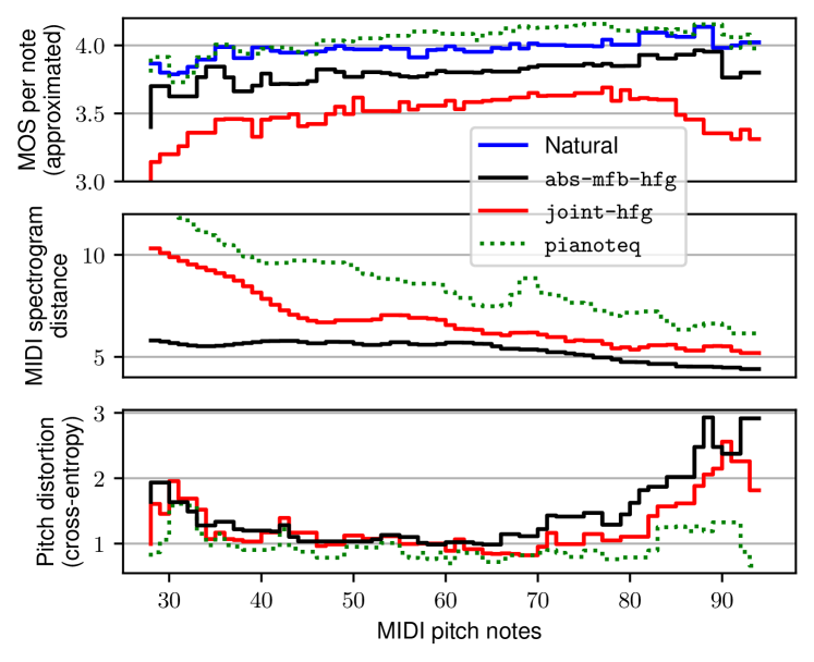
Fig. 4: Approximated MOS per note in test set (top panel), pitch distortion (middle panel), and MIDI-spec. distortion (bottom panel).

Figure 4 plots the results for joint-hfg, abs-mfb-hfg, and Pianoteq. It can be seen that the MOS of joint-hfg was below abs-mfb-hfg and the natural audio for all the evaluated notes, and it degraded more on low- and high-pitched notes. The gap may be due to the distortion in the spectra of the generated audio. Particularly, the MIDI spectrogram distortion of joint-hfg on the low-pitched notes was much higher than that of abs-mfb-hfg. Note that Pianoteq’s distortion was high because Pianoteq is based on another piano rather than the one that played the natural audio. On pitch distortion, joint-hfg was better than abs-mfb-hfg on most of the notes, especially those larger than 70. This is consistent with the gross pitch distortion in Table 1 and suggests that the gap between joint-hfg and abs-mfb-hfg may be mainly due to MIDI spectrogram distortion. However, notice that both joint-hfg and abs-mfb-hfg have a higher pitch distortion than Pianoteq, especially on high-pitched notes. Compared with the physical-model-based Pianoteq, the data-driven joint-hfg and abs-mfb-hfg need to further improve the pitch accuracy in order to boost the synthesized audio quality. Due to the space limitation, more objective analysis on inadequate MIDI spectrogram systems is available on our project webpage.

5 Conclusion

We synthesized high-fidelity piano audio from symbolic musical note input by modifying our previous TTS-based MIDI-to-audio system and introducing advanced TTS techniques. Even though a performance gap still remains between the best MIDI-to-audio system and the physical model-based software, our proposed system is more advantageous in terms of efficiency and flexibility. Through extensive analysis using subjective and objective evaluations, we measured the correlation between MOS and objective measurements, which indicates possibilities for further improvements in the future. Considering that we are able to synthesize highly natural-sounding music with TTS-based techniques, we also expect to investigate more areas related to music synthesis, such as timbre transfer, multi-instrument audio synthesis, and performance generation in our future work.

References

- [1] Erica Cooper, Xin Wang, and Junichi Yamagishi, “Text-to-speech synthesis techniques for MIDI-to-audio synthesis,” in Proc. SSW, 2021, pp. 130–135.
- [2] Hao-Wen Dong, Cong Zhou, Taylor Berg-Kirkpatrick, and Julian J. McAuley, “Deep performer: Score-to-audio music performance synthesis,” in Proc. ICASSP, 2022, pp. 951–955.
- [3] Bryan Wang and Yi-Hsuan Yang, “PerformanceNet: Score-to-audio music generation with multi-band convolutional residual network,” in Proc. AAAI, 2019, vol. 33, pp. 1174–1181.
- [4] Kundan Kumar, Rithesh Kumar, Thibault de Boissiere, Lucas Gestin, Wei Zhen Teoh, Jose Sotelo, Alexandre de Brébisson, Yoshua Bengio, and Aaron C Courville, “MelGAN: Generative adversarial networks for conditional waveform synthesis,” in Proc. NIPS, 2019, pp. 14910–14921.
- [5] Jong Wook Kim, Rachel Bittner, Aparna Kumar, and Juan Pablo Bello, “Neural music synthesis for flexible timbre control,” in Proc. ICASSP, 2019, pp. 176–180.
- [6] Yusong Wu, Ethan Manilow, Yi Deng, Rigel Swavely, Kyle Kastner, Tim Cooijmans, Aaron Courville, Cheng-Zhi Anna Huang, and Jesse Engel, “MIDI-DDSP: Detailed control of musical performance via hierarchical modeling,” in Proc. ICLR, 2022.
- [7] Tom Moebert, Josh Green, Pedro Lopez-Cabanillas, and David Henningsson, “FluidSynth,” https://www.fluidsynth.org.
- [8] MODARTT, “Pianoteq 7,” https://www.modartt.com/pianoteq.
- [9] Ondřej Cífka, Alexey Ozerov, Umut Şimşekli, and Gael Richard, “Self-supervised vq-vae for one-shot music style transfer,” in Proc. ICASSP, 2021, pp. 96–100.
- [10] Feynman T Liang, Mark Gotham, Matthew Johnson, and Jamie Shotton, “Automatic stylistic composition of Bach Chorales with deep LSTM.,” in Proc. ISMIR, 2017, pp. 449–456.
- [11] Erica Cooper, Cheng-I Lai, Yusuke Yasuda, Fuming Fang, Xin Wang, Nanxin Chen, and Junichi Yamagishi, “Zero-shot multi-speaker text-to-speech with state-of-the-art neural speaker embeddings,” in Proc. ICASSP, 2020, pp. 6184–6188.
- [12] Curtis Hawthorne, Ian Simon, Adam Roberts, Neil Zeghidour, Josh Gardner, Ethan Manilow, and Jesse Engel, “Multi-instrument music synthesis with spectrogram diffusion,” arXiv preprint arXiv:2206.05408, 2022.
- [13] Jesse Engel, Lamtharn (Hanoi) Hantrakul, Chenjie Gu, and Adam Roberts, “DDSP: Differentiable digital signal processing,” in Proc. ICLR, 2020.
- [14] Jonathan Shen, Ruoming Pang, Ron J Weiss, Mike Schuster, Navdeep Jaitly, Zongheng Yang, Zhifeng Chen, Yu Zhang, Yuxuan Wang, RJ Skerry-Ryan, and Others, “Natural TTS synthesis by conditioning WaveNet on Mel spectrogram predictions,” in Proc. ICASSP, 2018, pp. 4779–4783.
- [15] Jaehyeon Kim, Jungil Kong, and Juhee Son, “Conditional variational autoencoder with adversarial learning for end-to-end text-to-speech,” in Proc. ICML, 2021, pp. 5530–5540.
- [16] Xin Wang, Shinji Takaki, and Junichi Yamagishi, “Neural source-filter waveform models for statistical parametric speech synthesis,” IEEE/ACM Trans. on Audio, Speech, and Language Processing, vol. 28, pp. 402–415, 2019.
- [17] Naihan Li, Shujie Liu, Yanqing Liu, Sheng Zhao, and Ming Liu, “Neural speech synthesis with transformer network,” in Proc. AAAI, 2019, vol. 33, pp. 6706–6713.
- [18] Jungil Kong, Jaehyeon Kim, and Jaekyoung Bae, “HiFi-GAN: Generative Adversarial Networks for Efficient and High Fidelity Speech Synthesis,” in Proc. NIPS, 2020, vol. 33, pp. 17022–17033.
- [19] Daniel Griffin and Jae Lim, “Signal estimation from modified short-time fourier transform,” IEEE Trans. on acoustics, speech, and signal processing, vol. 32, no. 2, pp. 236–243, 1984.
- [20] Yusuke Yasuda, Xin Wang, Shinji Takaki, and Junichi Yamagishi, “Investigation of enhanced tacotron text-to-speech synthesis systems with self-attention for pitch accent language,” in Proc. ICASSP, 2019, pp. 6905–6909.
- [21] Cheng-Zhi Anna Huang, Ashish Vaswani, Jakob Uszkoreit, Ian Simon, Curtis Hawthorne, Noam Shazeer, Andrew M Dai, Matthew D Hoffman, Monica Dinculescu, and Douglas Eck, “Music Transformer: Generating music with long-term structure,” in Proc. ICLR, 2018.
- [22] Curtis Hawthorne, Andriy Stasyuk, Adam Roberts, Ian Simon, Cheng-Zhi Anna Huang, Sander Dieleman, Erich Elsen, Jesse Engel, and Douglas Eck, “Enabling factorized piano music modeling and generation with the MAESTRO dataset,” in Proc. ICLR, 2019.
- [23] Colin Raffel and Daniel P W Ellis, “Intuitive analysis, creation and manipulation of midi data with pretty midi,” in Proc. ISMIR late breaking and demo papers, 2014, pp. 84–93.
- [24] Tomoki Hayashi, Ryuichi Yamamoto, Katsuki Inoue, Takenori Yoshimura, Shinji Watanabe, Tomoki Toda, Kazuya Takeda, Yu Zhang, and Xu Tan, “Espnet-TTS: Unified, reproducible, and integratable open source end-to-end text-to-speech toolkit,” in Proc. ICASSP, 2020, pp. 7654–7658.
- [25] Yuxuan Wang, R. J. Skerry-Ryan, Daisy Stanton, Yonghui Wu, Ron J. Weiss, Navdeep Jaitly, Zongheng Yang, Ying Xiao, Zhifeng Chen, Samy Bengio, Quoc V. Le, Yannis Agiomyrgiannakis, Rob Clark, and Rif A. Saurous, “Tacotron: Towards end-to-end speech synthesis,” in Proc. Interspeech, 2017, pp. 4006–4010.
- [26] Florian Schmidt, “Generalization in generation: A closer look at exposure bias,” in Proc. Workshop on Neural Generation and Translation, 2019, pp. 157–167.
- [27] Diederik P Kingma and Jimmy Ba, “Adam: A method for stochastic optimization,” in Proc. ICLR, 2014.
- [28] Brian McFee, Colin Raffel, Dawen Liang, Daniel P W Ellis, Matt McVicar, Eric Battenberg, and Oriol Nieto, “librosa: Audio and music signal analysis in python,” in Proc. SciPy, 2015, pp. 18–25.
- [29] Jong Wook Kim, Justin Salamon, Peter Li, and Juan Pablo Bello, “CREPE: A convolutional representation for pitch estimation,” in Proc. ICASSP, 2018, pp. 161–165.