Fast Sampling of Diffusion Models via Operator Learning

Abstract

Diffusion models have found widespread adoption in various areas. However, their sampling process is slow because it requires hundreds to thousands of network evaluations to emulate a continuous process defined by differential equations. In this work, we use neural operators, an efficient method to solve the probability flow differential equations, to accelerate the sampling process of diffusion models. Compared to other fast sampling methods that have a sequential nature, we are the first to propose a parallel decoding method that generates images with only one model forward pass. We propose diffusion model sampling with neural operator (DSNO) that maps the initial condition, i.e., Gaussian distribution, to the continuous-time solution trajectory of the reverse diffusion process. To model the temporal correlations along the trajectory, we introduce temporal convolution layers that are parameterized in the Fourier space into the given diffusion model backbone. We show our method achieves state-of-the-art FID of 3.78 for CIFAR-10 and 7.83 for ImageNet-64 in the one-model-evaluation setting.

1 Introduction

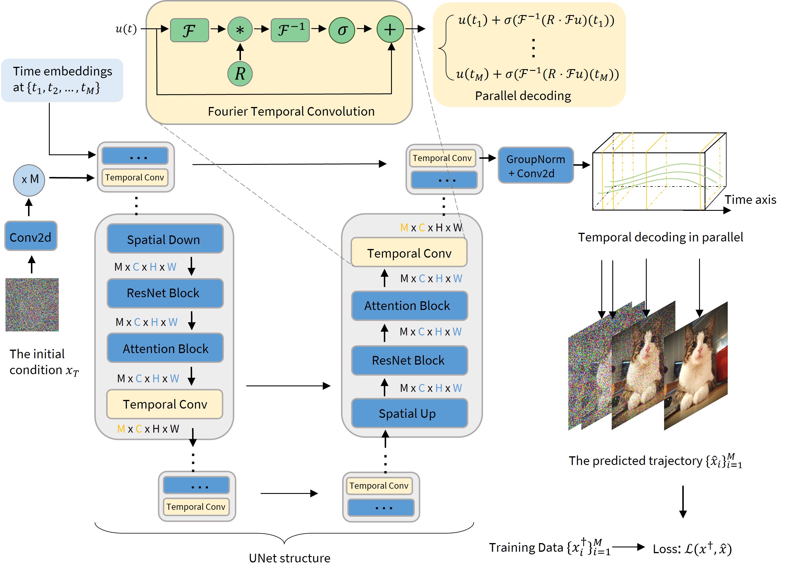
Figure 1: Illustration of the architecture and training pipeline of DSNO. The architecture of DSNO is built on top of any existing diffusion model architecture, where blue blocks are from the existing diffusion U-Net backbone and yellow blocks are the proposed temporal convolution layers. Suppose the temporal domain is discretized into $M$ points $\{t_{1},\dots,t_{M}\}$, for each feature map, the temporal convolution layers operate on the temporal and channel dimensions (M$\times$C) and the other blocks operate on the pixel and channel dimensions (C$\times$H$\times$W). The symbols ${\mathcal{F}}$ and ${\mathcal{F}}^{-1}$ refer to the Fourier transform and inverse Fourier transform, respectively. $R$ is a complex-valued parameter that represents a kernel function in Fourier space. For ease of notation, $x_{i}$ represents the solution at time $t_{i}$, that is $x(t_{i})$. Inside each temporal convolution layer, we apply the idea of parallel decoding: Given input function $u(t)$, the Fourier coefficients $R\cdot{\mathcal{F}}u$ is the same for all $t_{i},i=1,\dots,M$. Therefore, the temporal convolution layer can output the representations at different time locations in the trajectory in a single forward pass by evaluating the output function at queried points in parallel.

Diffusion models (Sohl-Dickstein et al., 2015; Ho et al., 2020), also known as score-based generative models (Song et al., 2020b), have emerged as a powerful generative modeling framework in various areas. They have achieved state-of-the-art (SOTA) performance in many applications including image generation (Dhariwal & Nichol, 2021), molecule generation (Xu et al., 2022), audio synthesis (Kong et al., 2021) and model robustness (Nie et al., 2022). However, sampling from diffusion models requires hundreds of neural network evaluations, making them slower by orders of magnitude compared to other generative models such as generative adversarial networks (GANs) (Goodfellow et al., 2020). Accelerating sampling in diffusion models remains a challenging but important problem, especially when applying them to time-sensitive downstream applications such as AI for art and design (Ramesh et al., 2022) or generative models for decision making (Ajay et al., 2022).

Existing methods for fast sampling of diffusion models can be summarized into two main categories: 1) training-free sampling methods (Song et al., 2020a; Lu et al., 2022) and 2) training-based sampling methods (Luhman & Luhman, 2021; Salimans & Ho, 2021; Xiao et al., 2021). Specifically, the training-free methods focus on reducing the number of discretization steps from a numerical perspective while solving the stochastic differential equations (SDE) or probability flow ordinary differential equations (ODE). However, even the best well-designed numerical solvers (Lu et al., 2022; Karras et al., 2022) still need 10$\sim$30 model evaluations such that the approximation error is small enough for an acceptable sampling quality. On the other hand, training-based methods train a surrogate network to replace some parts of the numerical solver or even the whole solver. Particularly, progressive distillation (Salimans & Ho, 2021) has made a big step towards real-time sampling (e.g., decent results with 4 steps) but it still has a sequential nature like conventional numerical solvers.

The goal of this work is to develop a fast and parallel sampling method for diffusion models with only one model evaluation. By parallel, we mean that our method can decode images at different time locations in the trajectory in parallel and hence, generate the final solution using only one model evaluation. The major challenge here arises from the difficulty of solving a complicated and large-scale differential equation, which typically requires many discrete time steps to emulate accurately from a numerical approximation perspective.

In this paper, we employ the recent advances in neural operators for solving differential equations to overcome this challenge. Neural operators (Li et al., 2020b; Kovachki et al., 2021b), especially the Fourier neural operator (FNO) (Li et al., 2020a) have shown several orders of magnitude speedup over conventional solvers. This class of models enables learning maps between spaces of functions and is shown to be discretization invariant, allowing them to work with different resolutions of data without changing the model parameters, and can approximate any given nonlinear continuous operator (Kovachki et al., 2021a).

The FNO allows for parallel decoding: i.e. the outputs at all locations of the trajectory can be simultaneously evaluated. This is a property that none of the previous sampling methods for diffusion models enjoy. In this work, we propose a neural operator for diffusion model sampling (DSNO) that maps the initial conditions (i.e. Gaussian distribution) to the solution trajectories and we show its effectiveness in both unconditional and class-conditional image generation.

Our contributions.

• We propose a neural operator for the fast sampling of diffusion models (DSNO) that can sample high-quality images with one model evaluation.

• We introduce temporal convolution blocks parameterized in Fourier space, which can be easily combined with any existing neural architectures of diffusion models to build a neural operator backbone for DSNO. Furthermore, our proposed temporal convolution blocks are lightweight and only increase the model size by 10%.

• For the first time, we propose a parallel decoding method to generate the trajectories of images using continuous function representation, which enables generation of the final solution in one model evaluation.

• Our proposed DSNO achieves new state-of-the-art FID scores of 3.78 for CIFAR-10 and 7.83 for ImageNet-64 in the setting of single-step-generation of diffusion models.

Finally, we note that DSNO leverages parallel decoding temporally to generate the solution trajectory by evaluating the output function at different time steps in parallel. This is in contrast to the prior training-based methods that have a sequential nature and predict the trajectory step by step. We believe that DSNO with parallel decoding is a key step for the real-time sampling of diffusion models, potentially benefiting many interactive applications.

2 Background

Score-based generative models.

We consider the general class of score-based generative models in a unified continuous-time framework proposed by Song et al. (2020b), which includes different variants of diffusion models (Sohl-Dickstein et al., 2015; Ho et al., 2020). In this paper, we will use the word score-based models interchangeably with diffusion models. Suppose the data distribution is $p_{\mathrm{data}}$. The forward pass is a diffusion process $\{{\mathbf{x}}(t)\}$ starting from $0$ to $T$ which can be expressed as

$$\mathrm{d}{\mathbf{x}}=f({\mathbf{x}},t)\mathrm{d}t+g(t)\mathrm{d}{\mathbf{w}}_{t},$$ (1)

where ${\mathbf{w}}_{t}$ is the standard Wiener process, and $f(\cdot,t):\mathbb{R}^{d}\rightarrow\mathbb{R}^{d}$ and $g(\cdot):\mathbb{R}\rightarrow\mathbb{R}$ are the drift and diffusion coefficients respectively. Diffusion models choose $f$ and $g$ such that ${\mathbf{x}}(0)\sim p_{\mathrm{data}}$ and ${\mathbf{x}}(T)\sim\mathcal{N}(0,\textbf{I})$. Song et al. (2020b) show that the following probability flow ODE produces the same marginal distributions $p_{t}({\mathbf{x}})$ as that of the diffusion process:

$$\mathrm{d}{\mathbf{x}}=f({\mathbf{x}},t)\mathrm{d}t-\frac{1}{2}g(t)^{2}\nabla_{{\mathbf{x}}}\log p_{t}({\mathbf{x}})\mathrm{d}t.$$ (2)

The sampling process eventually becomes solving the probability flow ODE 2 from $T$ to $0$ given the initial condition ${\mathbf{x}}(T)$. Furthermore, $f({\mathbf{x}},t)$ often has the affine form $f({\mathbf{x}},t)=h(t){\mathbf{x}}$, where $h:\mathbb{R}\rightarrow\mathbb{R}$. We can simplify the equation 2 into a semi-linear ODE. Integrating both sides over time gives the explicit form of solution for any $t<s$:

$${\mathbf{x}}(t)=\phi(t,s){\mathbf{x}}(s)-\int_{s}^{t}\phi(t,\tau)\frac{g(\tau)^{2}}{2}\nabla_{{\mathbf{x}}}\log p_{\tau}({\mathbf{x}})\mathrm{d}\tau,$$ (3)

where $\phi(t,s)=\exp\left(\int_{s}^{t}h(\tau)\mathrm{d}\tau\right)$. The ODE can be solved using numerical solvers such as Euler’s method, multistep methods, and Heun’s 2^nd method. The score function $\nabla_{{\mathbf{x}}}\log p_{t}({\mathbf{x}})$ is usually parameterized by $\hat{\epsilon}_{\theta}({\mathbf{x}}_{t})\approx-\sigma_{t}\nabla_{{\mathbf{x}}}\log p_{t}({\mathbf{x}})$, where $\sigma_{t}$ is the noise schedule (Song et al., 2020b; Ho et al., 2020).

Fourier neural operator.

Fourier neural operator (Li et al., 2020a) is one of the state-of-the-art data-driven methods for solving PDEs, which has shown great speedup over conventional PDE solvers in many scientific problems by learning a parametric map between two Banach spaces from data. They are constructed as a stack of kernel integration layers where the kernel function is parameterized by learnable weights. Let $D$ be a bounded domain, e.g., $[0,T]$ and $a:D\rightarrow\mathbb{R}^{d_{\mathrm{in}}}$ denote an input function. A Fourier neural operator ${\mathcal{G}}_{\theta}$, parameterized with learnable parameters $\theta$, is an $L$ layered neural operator of the following form,

$${\mathcal{G}}_{\theta}\coloneqq{\mathcal{Q}}\circ\sigma({\mathcal{W}}_{L}+{\mathcal{K}}_{L})\circ\dots\circ\sigma({\mathcal{W}}_{1}+{\mathcal{K}}_{1})\circ{\mathcal{P}},$$ (4)

where the lifting operator ${\mathcal{P}}$, projection operator ${\mathcal{Q}}$, and residual connections ${\mathcal{W}}_{i},i\in\{1,\dots,L\}$ are pointwise operators parameterized with neural networks, and $\sigma$ is a fixed nonlinear activation function. ${\mathcal{K}}_{i}$ is an integral kernel operator parameterized in Fourier space such that for a given $v_{i}$, an input function to the $i$’th layer, we have,

$$({\mathcal{K}}v_{i})(t)={\mathcal{F}}^{-1}\left(R_{i}\cdot({\mathcal{F}}v_{i})\right)(t),\forall t\in D$$ (5)

where ${\mathcal{F}}$ and ${\mathcal{F}}^{-1}$ are the Fourier transform and inverse Fourier transform on $D$, $R_{i}$ is a trainable parameter that parameterizes a kernel function in Fourier space. Given an input function $a$, we first apply the lifting point-wise operator ${\mathcal{P}}$ that expands the co-dimension of the input function $a$, followed by $L$ layers of global integral operators accompanied with pointwise non-linearity operation $\sigma$. The result of the global integration layers is passed to the local and pointwise projection layer ${\mathcal{Q}}$ to compute the output function. This architecture is shown to possess the crucial discretization invariance and universal approximation properties of universal operators (Kovachki et al., 2021a, b).

3 Learning the trajectory with neural operator

Problem statement.

Our goal is to learn a neural operator that given any initial condition ${\mathbf{x}}(T)\sim\mathcal{N}(0,\mathbf{I})$, predicts the probability flow trajectory $\{{\mathbf{x}}(t)\}_{s}^{0}$ with time flowing from $s$ to $0$ defined in equation 3, where the endpoint ${\mathbf{x}}(0)\in{\mathbb{R}}^{d}$ is the data. Let $D=[0,s],0<s\leq T$ be the temporal domain. Let $\mathcal{A}$ be the finite-dimensional space of the initial condition, and $\mathcal{U}=\mathcal{U}(D;\mathbb{R}^{d})$ denote the space of the target continuous time functions with output value in ${\mathbb{R}}^{d}$. We build a neural operator ${\mathcal{G}}_{\theta}$ parameterized by $\theta$ to approximate the solution operator ${\mathcal{G}}^{\dagger}$ by minimizing the error as follows

$$\min_{\theta}\mathbb{E}_{{\mathbf{x}}_{T}\sim{\mathcal{N}}(0,\mathbf{I})}{\mathcal{L}}\left({\mathcal{G}}_{\theta}\left({\mathbf{x}}_{T}\right)-{\mathcal{G}}^{\dagger}\left({\mathbf{x}}_{T}\right)\right),$$ (6)

where $\mathcal{L}:\mathcal{U}\rightarrow\mathbb{R}_{+}$ is some loss functional such as $L^{p}$-norm for some $p\geq 1$. From the exact solution ${\mathbf{x}}(t)$ in equation 3, we know the solution operator ${\mathcal{G}}^{\dagger}:\mathcal{A}\rightarrow\mathcal{U}$ exists and is a unique weighted integral operator of the score function. In other words, the solution operator corresponds to the underlying diffusion ODE, i.e., a mapping from a ${\mathbf{x}}(T)\sim\mathcal{N}(0,\mathbf{I})$ to the probability flow trajectory $\{{\mathbf{x}}(t)\}_{s}^{0}$. It is a regular operator, i.e., a member of operator set in the neural operator theory that can be approximated (Kovachki et al., 2021b, a). More formally,

Proposition 3.1 (Kovachki et al. (2021b, a)).

The class of neural operators defined in equation 4 approximates the solution map of the diffusion ODE, i.e., a mapping from ${\mathbf{x}}(T)\sim\mathcal{N}(0,\mathbf{I})$ to the probability flow trajectory $\{{\mathbf{x}}(t)\}_{s}^{0}$, arbitrarily well.

This implies that the proposed architecture has the required capacity to learn to output the continuous time probability flow trajectory $\{{\mathbf{x}}(t)\}_{s}^{0}$ in one model call.

Temporal convolution block in Fourier space.

Inspired by the weighted integral form of the exact ODE solution in equation 3, we build our temporal convolution block with Fourier integral operator $\mathcal{K}$ to efficiently model the trajectory. Given an input function $u:D\rightarrow{\mathbb{R}}^{d}$, our temporal convolution layer ${\mathcal{T}}$ is defined as

$$({\mathcal{T}}u)(t)=u(t)+\sigma\left(\left({\mathcal{K}}u\right)(t)\right),$$ (7)

where $\sigma$ is a point-wise nonlinear function, and ${\mathcal{K}}$ is a Fourier convolution operator defined in equation 5 parameterized by $R$. Note that our proposed temporal convolution layer differs slightly from the FNO layer given in equation 4. Specifically, we move the nonlinear activation function right after the Fourier convolution operator ${\mathcal{K}}$ and replace the linear pointwise operator ${\mathcal{W}}$ with an identity shortcut, which preserves the high-frequency information without extra cost and also leads to a better optimization landscape (He et al., 2016). We have not observed the advantages of using a more general linear layer. The identity map is shown to be sufficient and more attractive because it is computationally efficient. Furthermore, we note that, by convolution theorem, we have

$$({\mathcal{K}}u)(t)=\int_{D}(\mathcal{F}^{-1}R)(\tau)u(t-\tau)\mathrm{d}\tau,\forall t\in D.$$ (8)

Notably, the integral form in equation 8 inherently possesses a structural similarity to the core diffusion process in equation 3, meaning that the temporal convolution layer implicitly parameterize the ODE solution trajectory.

In practice, we use the discrete Fourier transforms for computational efficiency. Suppose the temporal domain $D$ is discretized into $M$ points. For ease of understanding, we also assume the codomains of the input and output functions of the temporal convolution block are both in ${\mathbb{R}}^{d}$. The input function $u(t)$ is represented as a tensor in ${\mathbb{R}}^{M\times d}$. $R$ is a complex-valued parameter in ${\mathbb{C}}^{J\times d\times d}$, where $J$ is the maximal number of modes that we can choose. For all $u$, we truncate the modes higher than $J$ and then have ${\mathcal{F}}(u)\in{\mathbb{C}}^{J\times d}$. The pointwise product of Fourier transforms of input and kernel functions is given by

$$R\cdot({\mathcal{F}}u)_{j,k}=\sum_{l=1}^{d}R_{j,k,l}({\mathcal{F}}u)_{j,l},$$ (9)

for all $j\in\{1,\dots,J\},k\in\{1,\dots,d\}$. Accordingly, ${\mathcal{F}}$ and ${\mathcal{F}}^{-1}$ are realized by the fast Fourier transform algorithm. Figure 1 demonstrates the implementation details of the temporal convolution layers. Note that the temporal convolution layer only operates over the temporal dimension and hidden feature channel dimension and thus treats the pixel dimension as the same as the batch dimension. In other words, $d$ in the above example corresponds to the number of channel dimensions in practice.

Architecture of DSNO.

As demonstrated in Figure 1, the architecture of DSNO is built on top of any existing architecture of diffusion models, by adding our proposed temporal convolution layers to each level of the U-Net structure. The dark blue blocks are the modules in the existing diffusion model backbone, which treat the temporal dimension the same as the batch dimension and only work on the pixel and channel dimension. The yellow blocks are the Fourier temporal convolution blocks, which only perform on the temporal and channel dimension. Therefore, our model is highly parallelizable and adds minimal computation complexity to the original backbone. Again, suppose the temporal domain is discretized into $\{t_{1},\dots,t_{M}\}$. The DSNO takes as input the time embeddings at these times and the initial condition. The feature map of the first convolution layer is repeated $M$ times over the temporal dimension as the initial feature at different times. Each feature representation is combined with the corresponding time embedding in the following ResNet blocks.

Training of DSNO

Training DSNO is a standard operator learning setting. The training objective is a weighted integral of the error:

$$\min_{\theta}\mathbb{E}_{{\mathbf{x}}_{T}\sim{\mathcal{N}}(0,\mathbf{I})}\int_{D}\lambda(t)\|{\mathcal{G}}_{\theta}({\mathbf{x}}_{T})(t)-{\mathcal{G}}^{\dagger}({\mathbf{x}}_{T})(t)\|\mathrm{d}t,$$ (10)

where $\theta$ is the parameter of DSNO, $\lambda(t)$ is the weighting function, ${\mathbf{x}}_{T}$ is the initial condition, and $\|\cdot\|$ is a norm. In practice, we optimize over $\theta$ to minimize the empirical-risk similar to  Kovachki et al. (2021b):

$$\min_{\theta}\frac{1}{N}\sum_{j=1}^{N}\frac{1}{M}\sum_{i=1}^{M}\lambda(t_{i})\|{\mathcal{G}}_{\theta}({\mathbf{x}}_{T}^{(j)})(t_{i})-{\mathcal{G}}^{\dagger}({\mathbf{x}}_{T}^{(j)})(t_{i})\|,$$ (11)

where $\{t_{1},\dots,t_{M}\}$ are discrete points in the temporal domain, and ${\mathcal{G}}^{\dagger}({\mathbf{x}}_{T}^{(j)})(t_{i})$ can be generated from any existing solver or sampling method.

Parallel decoding

As shown in the top two yellow blocks in Figure 1, the proposed Fourier temporal convolution block can predict images at different times in parallel. Given any input function $u(t)$, we can compute the Fourier coefficient $R\cdot{\mathcal{F}}u$ and then call the inverse Fourier transform at all $t_{i}$ in parallel to generate output for different times at once. Plus, the other modules of DSNO treat temporal dimension like batch dimension and can perform in parallel for different $t_{i}$s. Therefore, DSNO is capable of efficient parallel decoding. Note that the effectiveness of our parallel decoding is based on the fact that the solutions of the diffusion ODE at different times are conditionally independent given the initial condition. Parallel decoding has shown its efficiency in transformers-based models (Chang et al., 2023) and language models (Ghazvininejad et al., 2019) for discrete tokens generation in the spatial domain. DSNO is the first parallel decoding method for continuous diffusion ODE trajectory, which is in temporal domain.

Compact power spectrum.

We examine the spectrum of the probability flow ODE trajectories generated from several publicly available pre-trained diffusion models in the literature, and observe that the ODE trajectories always have a compact energy spectrum over the temporal dimension. See more details in Appendix A.1. The smoothness of the diffusion ODE trajectory means the high-frequency modes do not contribute much to the learning objective. Therefore, DSNO built upon the stacks of Fourier temporal convolution layers can model the underlying solution operator of diffusion ODEs more efficiently with a relatively small number of discretization steps $M$.

Table 1: Comparison of fast sampling methods on CIFAR-10 for diffusion models in the literature. The FID score is computed with the original FID implementation to compare with the other methods. NFE: number of function evaluations.

Method	NFE	FID	Model size
Ours	1	3.78	65.8M
Knowledge distillation
(Luhman & Luhman, 2021)	1	9.36	35.7M
Progressive distillation
(Salimans & Ho, 2021)	1	9.12	60.0M
	2	4.51
	4	3.00
LSGM (Vahdat et al., 2021)	147	2.10	475.0M
GGDM + PRED + TIME
(Watson et al., 2021)	5	13.77	35.7M
	10	8.23
DDIM (Song et al., 2020a)	10	13.36	35.7M
	20	6.84
	50	4.67
SN-DDIM (Bao et al., 2022)	10	12.19	52.6M
FastDPM (Kong & Ping, 2021)	10	9.90	35.7M
DPM-solver (Lu et al., 2022)	10	4.70	35.7M
DEIS (Zhang & Chen, 2022)	10	4.17	-
Diffusion + GAN
TDPM (Zheng et al., 2022)	5	3.34	35.7M
DDGAN (Xiao et al., 2021)	4	3.75	-

4 Experiments

In our experiments, we examine the proposed method on both unconditional and conditional image generation tasks. We show that our method dramatically accelerates the sampling process of diffusion models, compared to existing fast sampling methods including both training-free and training-based approaches. Our code is available at https://github.com/devzhk/DSNO-pytorch.

Table 2: Comparison of fast sampling methods on class-conditional ImageNet-64 for diffusion models in the literature. The results of DDIM and EDM are reported by Karras et al. (2022) using the pre-trained model (Dhariwal & Nichol, 2021).

Method	Model evaluations	FID score	Recall	Model size
Ours	1	7.83	0.61	329.2M
Progressive distillation (Salimans & Ho, 2021)	1	15.99	0.60	295.9M
	2	7.11	0.63
	4	3.84	0.63
EDM (Karras et al., 2022)	79	2.44	0.67	295.9M
DDIM (Song et al., 2020a)	32	5.00	-	295.9M
BigGAN-deep (Brock et al., 2018)	1	4.06	0.48
ADM (Dhariwal & Nichol, 2021)	250	2.07	0.63	295.9M

Table 3: One model evaluation cost tested on V100. We compare the time cost of a single forward pass of DSNO and the corresponding original backbone. The reported results are averaged over 20 runs. The baseline models are from Salimans & Ho (2021).

Backbone	Runtime	Model size
CIFAR-10	0.033s	60.00M
DSNO-CIFAR-10 (ours)	0.050s	65.77M
ImageNet64	0.066s	295.90M
DSNO-ImageNet-64 (ours)	0.080s	329.23M

4.1 Experimental setup

We first randomly sample a training set of ODE trajectories using the pre-trained diffusion model to be distilled. We then build the network backbone for DSNO by simply adding the proposed temporal convolution layers to the above diffusion model. We initialize the modules from the existing architecture with the pre-trained weights. As for the activation function in the temporal convolution layer, we use the leaky rectified linear unit (LeakyReLU) for $\sigma$. We mainly use $\ell^{1}$ loss for the experiments on CIFAR10 and ImageNet-64. We also experiment with LPIPS (Zhang et al., 2018) loss on CIFAR10 like one concurrent work (Song et al., 2023) does. Regarding the choice of the loss weighting function, we set $\lambda(t)=\frac{\alpha_{t}}{\sigma_{t}}$, which is the square root of the SNR loss weighting used in the original diffusion model (Salimans & Ho, 2021). We take the square root because our loss function is not squared. We use a batch size of 256 for CIFAR-10 experiments, a batch size of 2048 for ImageNet experiments, and a batch size of 128 by default in our ablation study. We use the same base learning rate of 0.0002, learning rate warmup schedule, and $\beta_{1},\beta_{2}$ of Adam (Kingma & Ba, 2014) as used in the diffusion model training without tuning these hyperparameters.

Evaluation metric

We use the Frechet inception distance (FID) (Heusel et al., 2017) to evaluate the quality of generated images. FID score is computed by comparing 50,000 generated images against the corresponding reference statistics of the dataset. We use the ADM’s TensorFlow evaluation suite (Dhariwal & Nichol, 2021) and EDM’s evaluation code (Karras et al., 2022) to compute FID-50K with the same reference statistics. We also report Recall (Kynkäänniemi et al., 2019) as the secondary metric of mode coverage for the experiments on ImageNet-64.

4.2 Unconditional generation: CIFAR-10

Trajectory data collection.

We first generate 1 million trajectories with 512-step DDIM (Song et al., 2020a) using the pre-trained diffusion model proposed by Salimans & Ho (2021), and use it to train DSNO. The FID score of the training set is 2.51, computed over the first 50k data points in the training set.

Sampling quality and speed.

Table 1 compares the proposed DSNO trained with a temporal resolution of 4 against both training-based and training-free sampling methods in terms of FID and the corresponding number of model evaluations. DSNO clearly outperforms all the baselines with only one model evaluation and even achieves a better FID score than 2-step progressive distillation models. Furthermore, we compare the cost of one single forward pass of both DSNO and the original backbone on a V100 in a standard AWS p3.2xlarge instance. For the speed test, we do 20 warm-up runs to avoid the potential inconsistency arising from the built-in cudnn autotuner. Since the time cost of progressive distillation grows linearly with the number of sampling steps, we can easily calculate the speedup of DSNO over the progressive distillation from Table 3. DSNO is 2.6 times faster than the 4-step progressive distillation model and 1.3 times faster than 2-step progressive distillation model. Compared to hybrid models that combine GAN and diffusion models, DSNO achieves comparable performance with at most one-fourth number of model evaluations.

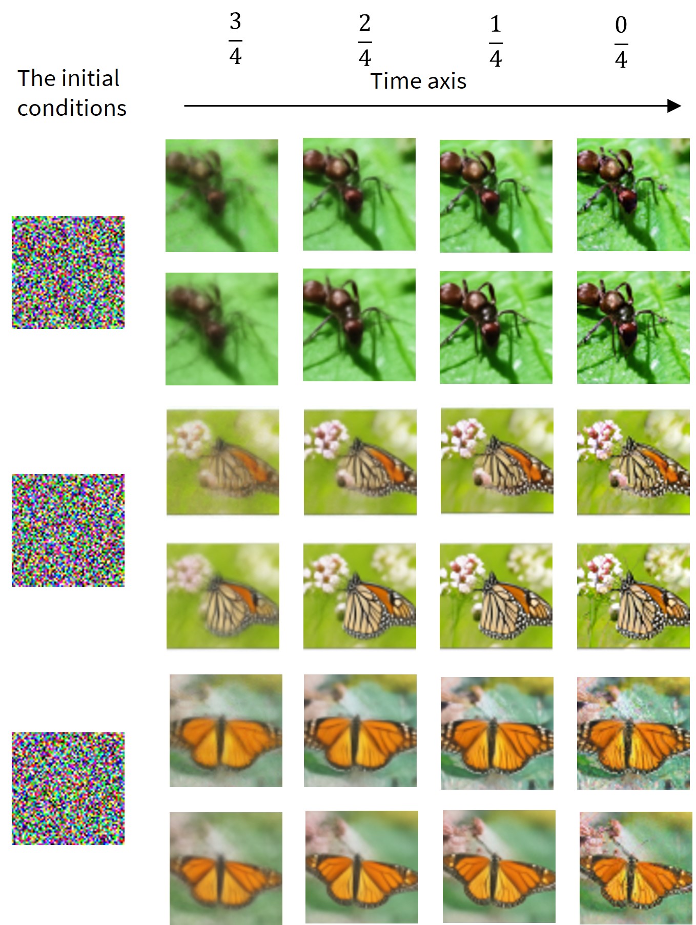
Figure 2: Comparison between the trajectory predicted by DSNO and that from the original solver on ImageNet-64, for the fixed random seed with a temporal resolution 4. Upper row: the prediction by DSNO. Lower row: the trajectory generated by solver.

4.3 Conditional generation: ImageNet-64

Trajectory data collection.

We generate 2.3 million trajectories with 16-step progressive distillation (Salimans & Ho, 2021) using the pre-trained diffusion model from its official code base. The FID score of the generated training set is 2.70, computed over the first 50k training data points.

Sampling quality and speed.

Table 2 compares DSNO trained with a temporal resolution of 4 against the recent advanced fast sampling methods for diffusion models. DSNO clearly outperforms 1-step progressive distillation model and archives comparable FID 2-step models of progressive distillation with only one model evaluation. From Table 3, DSNO has 1.7 times speedup over progressive distillation. The recall of DSNO is comparable to ADM’s, showing that DSNO inherits the original diffusion model’s diversity/mode coverage as it learns to solve the probability flow ODE.

Trajectory prediction and reconstruction.

Figure 2 compares the trajectories predicted by DSNO and the original ODE solver, respectively, for the fixed random seed with a temporal resolution 4. We see that the DSNO predicted trajectory highly matches the groundth-truth ODE trajectory, which demonstrates the effectiveness of DSNO with parallel decoding. Besides, Figure 3 shows the random samples from DSNO and the original pre-trained diffusion model with the same random seed. It is clear that the mapping from Gaussian noise to the output image is well-preserved.

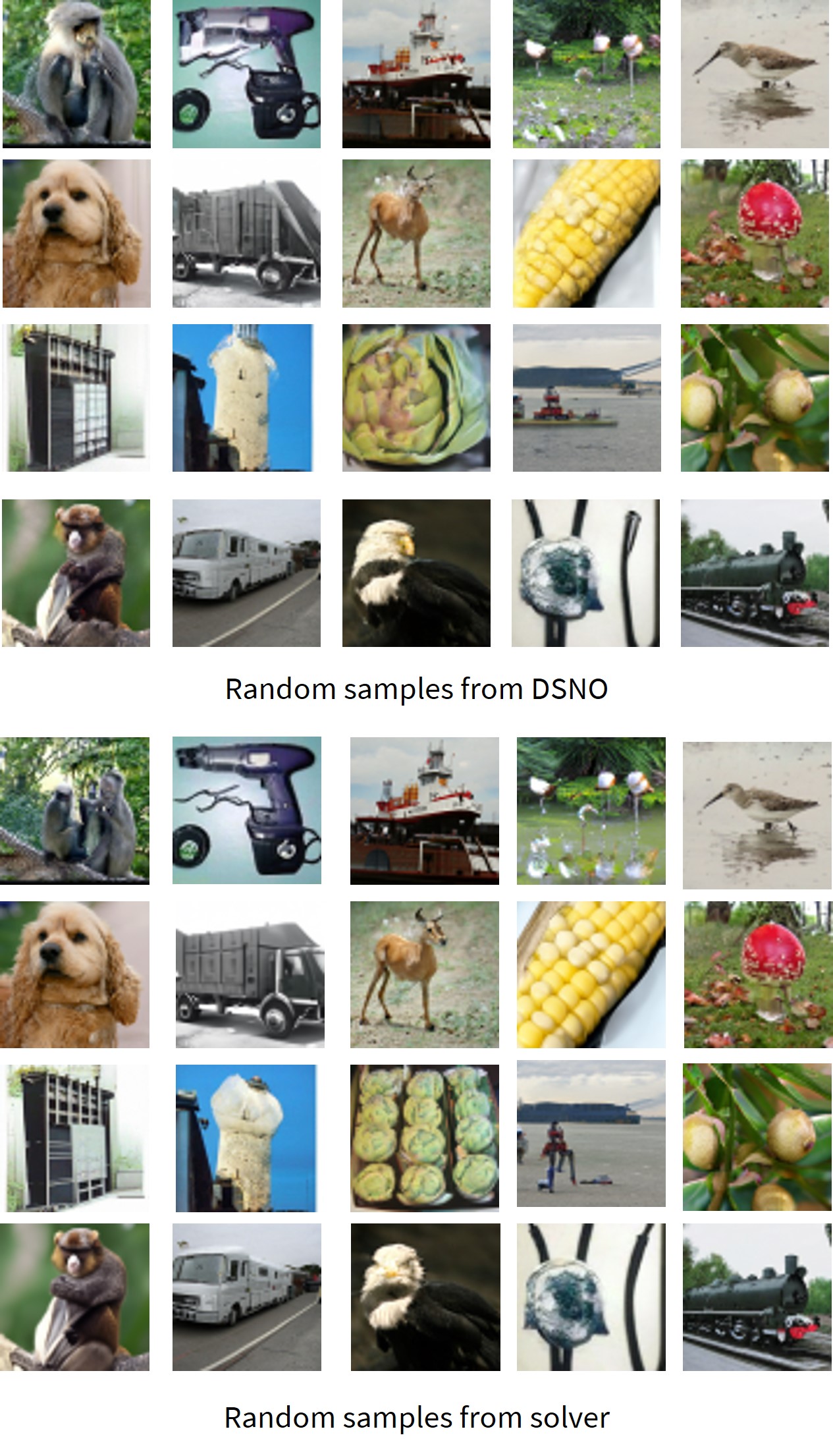
Figure 3: Upper panel: random samples generated by DSNO. Bottom panel: generated by the solver.

Table 4: Impact of temporal convolution. We compare the performance of architectures with and without temporal convolution blocks while keeping all other settings the same.

Training steps	U-Net	U-Net + Temporal Conv
300k	8.09	4.23
400k	7.85	4.12

Table 5: Ablation study on the choice of training loss weighting and time discretization scheme. The temporal resolution is fixed to 4 in this group of experiments.

Loss weighting	Uniform	$\mathrm{SNR}^{0.5}$
FID	4.56	4.21
time discretization scheme	Uniform	Quadratic
FID	4.33	4.21

Table 6: Ablation study on the choice of the temporal resolution.

Temporal resolution	2	4	8
FID	5.01	4.21	3.98

4.4 Ablation study

In this section, we study the effect of different model choices, including the temporal convolution blocks, loss weighting function, temporal resolution, time discretization scheme, and loss function, by performing ablation studies on CIFAR-10. Without stated explicitly, we use batch size 128 and $\ell^{1}$ norm for the loss function.

Temporal convolution block.

We first investigate the impact of temporal convolution by comparing the performance of architectures with and without temporal convolution blocks. All the other settings are kept the same such as temporal resolution 4, quadratic time discretization scheme, the square root of the SNR weighting function, and batch size 256. As reported in Table 4, the temporal convolution design is crucial to DSNO’s performance as its kernel integration operator nature is a better model inductive bias to model the trajectory in time.

Loss weighting.

The loss weighting function used in the training objective of Diffusion models(Ho et al., 2020; Song et al., 2020b) typically distributes more weights to the small times, which is important to training diffusion models. We also adopt such a weighting function since it is generally harder to control the error at small times. We observe that such loss weighting function benefits the training of DSNO. As reported in Table 5, using the square root of the SNR weighting function slightly improves the FID by 0.35.

Time discretization scheme.

How to discretize the temporal domain is important to the performance of the numerical solvers. Some small changes to the time discretization scheme could lead to very different sample qualities as shown in (Karras et al., 2022; Zhang & Chen, 2022). DSNO also needs to choose a way to discretize the temporal domain. Here we consider the two most common choices of time discretization schemes in the literature: uniform time step and quadratic time step. As shown in Table 5, the quadratic time step is slightly better than the uniform time step by 0.12, showing that DSNO is not sensitive to the different time discretization schemes used in the existing solvers and can work nicely with different solvers.

Temporal resolution.

We study the effect of temporal resolution (i.e., the discretization steps $M$), given the square root of SNR weighting function and the quadratic time discretization scheme. As reported in Table 6, the FID improves as we increase the temporal resolution. Since the higher temporal resolution introduces more supervision into the training, it is reasonable to expect better FID scores. However, higher resolution also results in higher computation costs. Since increasing the resolution from 4 to 8 only provides a marginal benefit (due to the compact spectrum we observed in Appendix A.1), one may use temporal resolution 4 for better efficiency.

Table 7: Ablation study on the choice of the loss function. For LPIPS, we use the original VGG-based version without any calibration (Zhang et al., 2018).

Loss function	$\ell^{1}$	LPIPS
FID	4.12	3.78

Loss function.

We only vary the loss function but keep the other settings the same, including a batch size of 256, a temporal resolution of 4, and a quadratic discretization scheme. As shown in Table 7, using the original VGG-based LPIPS loss (Zhang et al., 2018) instead of the standard $\ell^{1}$ loss leads to a further improvement in the FID score.

5 Related work

ODE-based sampling.

ODE-based samplers are much more widely used in practice (Rombach et al., 2022) than SDE-based methods because they can take large time steps by leveraging some useful structures of the underlying ODE such as semi-linear structure and the form of exponentially weighted integral (Lu et al., 2022; Zhang & Chen, 2022). Existing works (Song et al., 2021; Bao et al., 2021; Zhang & Chen, 2022; Dockhorn et al., 2022) have greatly reduced the number of discretization steps to 10-50 in time while keeping the approximation error small to generate high-quality samples. The exponentially weighted integral structure of the solution trajectory revealed by prior works also inspired our design of the temporal convolution block.

Operator learning for solving PDEs.

Neural operators are deep learning models that are designed for mappings between function spaces, i.e., continuous functions (Li et al., 2020b; Kovachki et al., 2021a). They are widely deployed as the de facto deep learning models in scientific computing when dealing with partial differential equations (PDE). Among these methods, Fourier neural operator stands out and is one of the most efficient machine learning methods for scientific computing problems involving PDE (Yang et al., 2021; Wen et al., 2022). It is shown to possess the crucial discretization invariance and universal approximation properties of universal operators (Kovachki et al., 2021a, b), which motivates our design of the temporal convolution block in our method.

Training-based sampling.

Training-based methods typically train a neural network surrogate to replace some parts of the numerical solver or even the whole solver. This category includes various methods from diverse perspectives such as knowledge distillation (Luhman & Luhman, 2021; Salimans & Ho, 2021), learning the noise schedule (Lam et al., 2021; Watson et al., 2021), learning the reverse covariance (Bao et al., 2022), which require extra training. Training-based methods usually work in the few-step regime with less than 10 steps. Direct Luhman & Luhman (2021) is the first work to get descent sample quality on CIFAR10 with one model evaluation but it suffers from overfitting and its sampling quality drops dramatically compared to the original sampling methods of diffusion models. The current SOTA progressive distillation (Salimans & Ho, 2021) reduces the number of steps down to 4-8 without losing much sample quality. However, it has the same issue as knowledge distillation in the limit of one function evaluation. Some other methods (Xiao et al., 2021; Vahdat et al., 2021; Zheng et al., 2022) combine diffusion models with other generative models such as GAN and VAE to enable fast sampling.

6 Conclusion and discussion

In this paper, we propose diffusion model sampling with neural operator (DSNO) that maps the initial condition, i.e., Gaussian distribution, to the continuous-time solution trajectory of the reverse diffusion process. To better model the temporal correlations along the trajectory, we introduce temporal convolution layers into the given diffusion model backbone. Experiments show that our method achieves the SOTA FID score of 3.78 for CIFAR-10 and 7.83 for ImageNet-64 with only one model evaluation. Our method is a big step toward real-time sampling of diffusion models, which can potentially benefit many time-sensitive applications of diffusion models.

Appendix A Appendix

A.1 Energy spectrum

The discrete-time Fourier transform of the signal $x(t)$ with period $T$ is given by

$$X_{j}=\sum_{i=1}^{N}x(t_{i})\exp\left(-\frac{2\pi}{T}jit_{i}\right),$$ (12)

where $t_{i}=\frac{iT}{N}$. $\frac{j}{T}$ is the frequency. $j$ is called the frequency mode. Let $\Delta=\frac{1}{N}$ be the time step. The spectrum is defined as the product of the Fourier transform of $x$ with its conjugate:

$$S_{j}=\frac{2\Delta^{2}}{T}X_{j}X_{j}^{*},$$ (13)

where $X_{j}^{*}$ is the complex conjugate. In practice, the statistics are computed over all pixel locations and channels of randomly generated trajectories. $T=1$ and the sampling frequency is 1000 Hz to avoid aliasing. Figure 4 visualizes the energy spectrum of ODE trajectories sampled from the diffusion model ”DDPM++ cont. (VP)” trained by (Song et al., 2020b) on CIFAR10. We observe that most power concentrates in the regime where the frequency mode is less than 5.

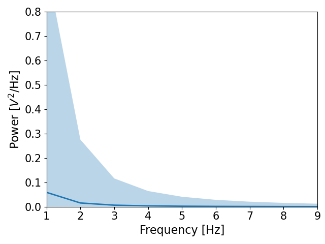
Figure 4: Power spectrum of the ODE trajectories sampled from ”DDPM++ cont. (VP)” model trained by (Song et al., 2020b) on CIFAR10. The mean is computed over all pixel locations and channels of randomly generated trajectories. Most power concentrates in the $\leq 5$ Hz regime. The shaded region represents the maximum and minimum power.

A.2 Background: neural operators

Let $\mathcal{A}$ and $\mathcal{U}$ be two Banach spaces and $G:\mathcal{A}\rightarrow\mathcal{U}$ be a non-linear map. Suppose we have a finite collection of data $\{a_{i},u_{i}\}_{i=1}^{N}$ where $a_{i}\sim\mu$ are i.i.d. samples from the distribution $\mu$ supported on $\mathcal{A}$ and $u_{i}=G(a_{i})$. Neural operators aim to learn $G_{\phi}$ parameterized by $\phi$ to approximate $G$ from the observed data by minimizing the empirical risk given by

$$\min_{\phi}\mathbb{E}_{a\sim\mu}\|G(a)-G_{\phi}(a)\|_{\mathcal{U}}\approx\min_{\phi}\frac{1}{N}\sum_{i=1}^{N}\|u_{i}-G_{\phi}(a_{i})\|_{\mathcal{U}}.$$ (14)

The architecture of neural operators is constructed as a stack of kernel integration layers where the kernel function is parameterized by learnable weights. This architecture utilizes the convolution theorem on abelian groups. Among different neural operator architectures, Fourier neural operator (Li et al., 2020a) stands out and is one of the most efficient machine learning methods for scientific computing problems involving PDE (Yang et al., 2021; Wen et al., 2022). It is shown to possess the crucial discretization invariance and universal approximation properties of universal operators (Kovachki et al., 2021a, b).

A.3 Extended set of generated samples

We provide an extended set of randomly generated samples from our ImageNet-64 model in Figure 5.

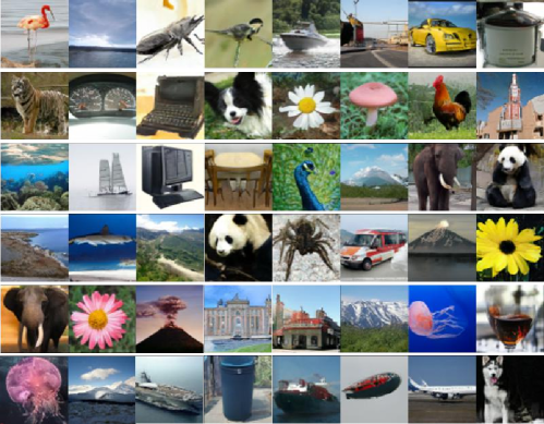
Figure 5: Random samples generated from DSNO on ImageNet-64.

A.4 Generalization to different resolution

Figure 6 visualizes the predicted trajectory of DSNO in temporal resolution 8 on ImageNet-64 while it is trained on temporal resolution 4. Although the resulting trajectories do not look perfectly smooth, it still demonstrates the generalization ability of DSNO to unseen time resolutions.

A.5 Further discussion

Future work

There are several directions we leave as future work. First, guided sampling of diffusion models is widely used in various applications but accelerating guided sampling is also more challenging (Meng et al., 2022). How to adapt DSNO for sampling Guided diffusion model will be an interesting next step. Second, the temporally continuous output of DSNO provides another level of flexibility compared to distillation-based methods and is readily available for applications such as DiffPure (Nie et al., 2022) that require fast forward/backward sampling from diffusion models at various temporal locations. DSNO could potentially reduce the inference time in those applications. We leave the exploration of those applications to future work. Last but not least, transformer-based architectures have shown their promising capacity for diffusion models (Peebles & Xie, 2022; Bao et al., 2023) in high-resolution image generation. It is natural to integrate our temporal convolution layers into these diffusion transformers as the temporal blocks operate solely on the temporal dimension regardless of how the pixel space is modeled. The resulting new architecture could also potentially serve as a new architecture design for other problems where the dynamics are continuous in time.

Reducing data collection cost with advanced solvers.

While we primarily use DDIM solver to collect data for fair comparison in this paper, it is worth noting that advanced numerical solvers like DPM solver(Lu et al., 2022) can approximate the solution operator with less computation cost, which will greatly speed up our training data generation process. Our final implementation includes examples of using DPM solvers in our GitHub repository https://github.com/devzhk/DSNO-pytorch.

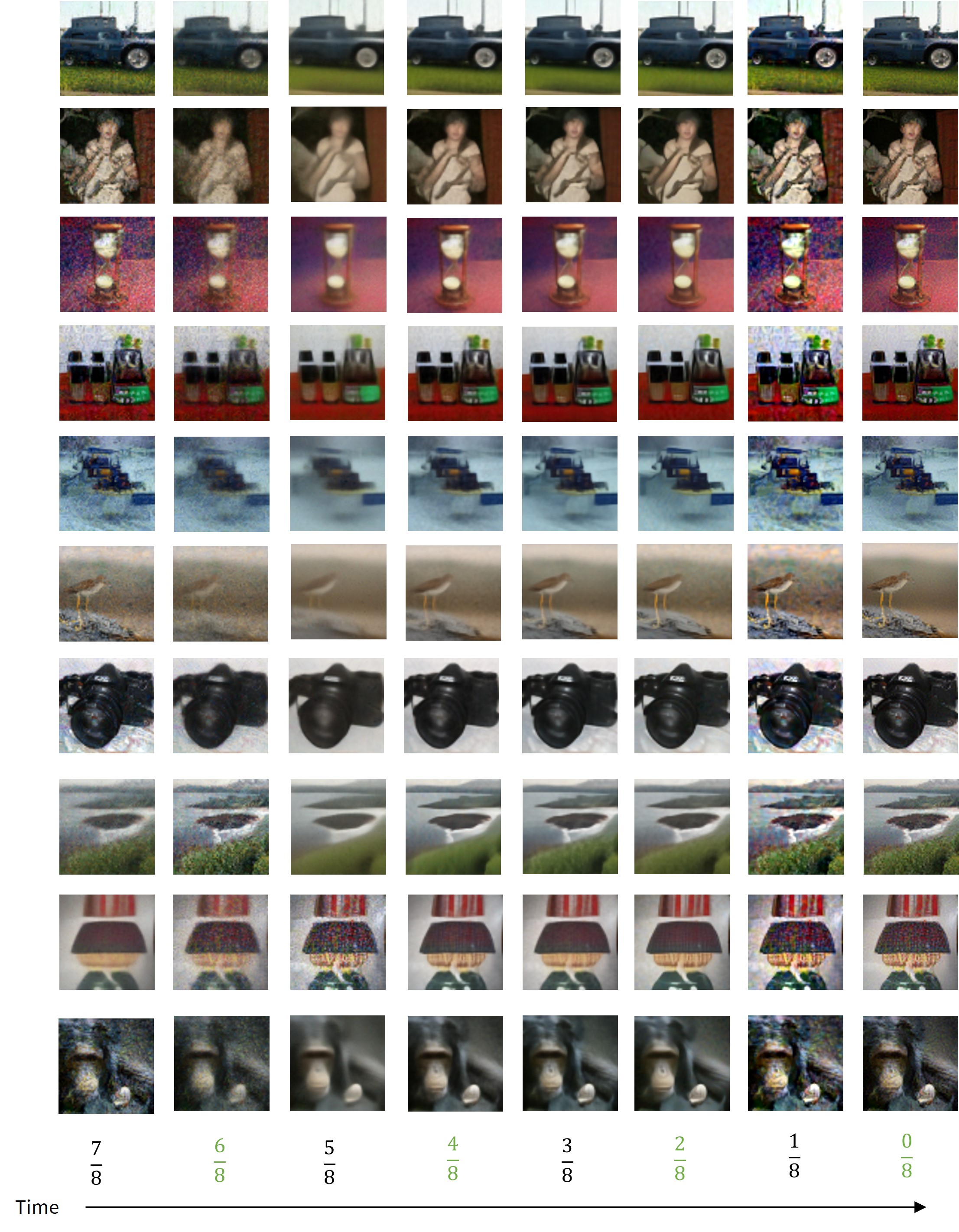
Figure 6: The predicted trajectory of DSNO with a temporal resolution of 8 on ImageNet-64. We train the DSNO with a temporal resolution of 4 and then use it to predict the trajectory with a temporal resolution of 8. Time locations marked green are the points that DSNO is trained with. Black time locations are the points that DSNO never saw in the training set.

References

- Ajay et al. (2022) Ajay, A., Du, Y., Gupta, A., Tenenbaum, J., Jaakkola, T., and Agrawal, P. Is conditional generative modeling all you need for decision-making? arXiv preprint arXiv:2211.15657, 2022.
- Bao et al. (2021) Bao, F., Li, C., Zhu, J., and Zhang, B. Analytic-dpm: an analytic estimate of the optimal reverse variance in diffusion probabilistic models. In International Conference on Learning Representations, 2021.
- Bao et al. (2022) Bao, F., Li, C., Sun, J., Zhu, J., and Zhang, B. Estimating the optimal covariance with imperfect mean in diffusion probabilistic models. arXiv preprint arXiv:2206.07309, 2022.
- Bao et al. (2023) Bao, F., Nie, S., Xue, K., Cao, Y., Li, C., Su, H., and Zhu, J. All are worth words: A vit backbone for diffusion models. In Proceedings of the IEEE/CVF Conference on Computer Vision and Pattern Recognition, pp. 22669–22679, 2023.
- Brock et al. (2018) Brock, A., Donahue, J., and Simonyan, K. Large scale gan training for high fidelity natural image synthesis. arXiv preprint arXiv:1809.11096, 2018.
- Chang et al. (2023) Chang, H., Zhang, H., Barber, J., Maschinot, A., Lezama, J., Jiang, L., Yang, M.-H., Murphy, K., Freeman, W. T., Rubinstein, M., et al. Muse: Text-to-image generation via masked generative transformers. arXiv preprint arXiv:2301.00704, 2023.
- Dhariwal & Nichol (2021) Dhariwal, P. and Nichol, A. Diffusion models beat gans on image synthesis. Advances in Neural Information Processing Systems, 34:8780–8794, 2021.
- Dockhorn et al. (2022) Dockhorn, T., Vahdat, A., and Kreis, K. GENIE: Higher-Order Denoising Diffusion Solvers. In Advances in Neural Information Processing Systems, 2022.
- Ghazvininejad et al. (2019) Ghazvininejad, M., Levy, O., Liu, Y., and Zettlemoyer, L. Mask-predict: Parallel decoding of conditional masked language models. arXiv preprint arXiv:1904.09324, 2019.
- Goodfellow et al. (2020) Goodfellow, I., Pouget-Abadie, J., Mirza, M., Xu, B., Warde-Farley, D., Ozair, S., Courville, A., and Bengio, Y. Generative adversarial networks. Communications of the ACM, 63(11):139–144, 2020.
- He et al. (2016) He, K., Zhang, X., Ren, S., and Sun, J. Deep residual learning for image recognition. In Proceedings of the IEEE conference on computer vision and pattern recognition, pp. 770–778, 2016.
- Heusel et al. (2017) Heusel, M., Ramsauer, H., Unterthiner, T., Nessler, B., and Hochreiter, S. Gans trained by a two time-scale update rule converge to a local nash equilibrium. Advances in neural information processing systems, 30, 2017.
- Ho et al. (2020) Ho, J., Jain, A., and Abbeel, P. Denoising diffusion probabilistic models. Advances in Neural Information Processing Systems, 33:6840–6851, 2020.
- Karras et al. (2022) Karras, T., Aittala, M., Aila, T., and Laine, S. Elucidating the design space of diffusion-based generative models. arXiv preprint arXiv:2206.00364, 2022.
- Kingma & Ba (2014) Kingma, D. P. and Ba, J. Adam: A method for stochastic optimization. arXiv preprint arXiv:1412.6980, 2014.
- Kong & Ping (2021) Kong, Z. and Ping, W. On fast sampling of diffusion probabilistic models. arXiv preprint arXiv:2106.00132, 2021.
- Kong et al. (2021) Kong, Z., Ping, W., Huang, J., Zhao, K., and Catanzaro, B. Diffwave: A versatile diffusion model for audio synthesis. In ICLR, 2021.
- Kovachki et al. (2021a) Kovachki, N., Lanthaler, S., and Mishra, S. On universal approximation and error bounds for fourier neural operators. Journal of Machine Learning Research, 22:Art–No, 2021a.
- Kovachki et al. (2021b) Kovachki, N., Li, Z., Liu, B., Azizzadenesheli, K., Bhattacharya, K., Stuart, A., and Anandkumar, A. Neural operator: Learning maps between function spaces. arXiv preprint arXiv:2108.08481, 2021b.
- Kynkäänniemi et al. (2019) Kynkäänniemi, T., Karras, T., Laine, S., Lehtinen, J., and Aila, T. Improved precision and recall metric for assessing generative models. Advances in Neural Information Processing Systems, 32, 2019.
- Lam et al. (2021) Lam, M. W., Wang, J., Huang, R., Su, D., and Yu, D. Bilateral denoising diffusion models. arXiv preprint arXiv:2108.11514, 2021.
- Li et al. (2020a) Li, Z., Kovachki, N., Azizzadenesheli, K., Liu, B., Bhattacharya, K., Stuart, A., and Anandkumar, A. Fourier neural operator for parametric partial differential equations. arXiv preprint arXiv:2010.08895, 2020a.
- Li et al. (2020b) Li, Z., Kovachki, N., Azizzadenesheli, K., Liu, B., Bhattacharya, K., Stuart, A., and Anandkumar, A. Neural operator: Graph kernel network for partial differential equations. arXiv preprint arXiv:2003.03485, 2020b.
- Lu et al. (2022) Lu, C., Zhou, Y., Bao, F., Chen, J., Li, C., and Zhu, J. Dpm-solver: A fast ode solver for diffusion probabilistic model sampling in around 10 steps. arXiv preprint arXiv:2206.00927, 2022.
- Luhman & Luhman (2021) Luhman, E. and Luhman, T. Knowledge distillation in iterative generative models for improved sampling speed. arXiv preprint arXiv:2101.02388, 2021.
- Meng et al. (2022) Meng, C., Gao, R., Kingma, D. P., Ermon, S., Ho, J., and Salimans, T. On distillation of guided diffusion models. arXiv preprint arXiv:2210.03142, 2022.
- Nie et al. (2022) Nie, W., Guo, B., Huang, Y., Xiao, C., Vahdat, A., and Anandkumar, A. Diffusion models for adversarial purification. In International Conference on Machine Learning (ICML), 2022.
- Peebles & Xie (2022) Peebles, W. and Xie, S. Scalable diffusion models with transformers. arXiv preprint arXiv:2212.09748, 2022.
- Ramesh et al. (2022) Ramesh, A., Dhariwal, P., Nichol, A., Chu, C., and Chen, M. Hierarchical text-conditional image generation with clip latents. arXiv preprint arXiv:2204.06125, 2022.
- Rombach et al. (2022) Rombach, R., Blattmann, A., Lorenz, D., Esser, P., and Ommer, B. High-resolution image synthesis with latent diffusion models. In Proceedings of the IEEE Conference on Computer Vision and Pattern Recognition (CVPR), 2022. URL https://github.com/CompVis/latent-diffusionhttps://arxiv.org/abs/2112.10752.
- Salimans & Ho (2021) Salimans, T. and Ho, J. Progressive distillation for fast sampling of diffusion models. In International Conference on Learning Representations, 2021.
- Sohl-Dickstein et al. (2015) Sohl-Dickstein, J., Weiss, E., Maheswaranathan, N., and Ganguli, S. Deep unsupervised learning using nonequilibrium thermodynamics. In International Conference on Machine Learning, pp. 2256–2265. PMLR, 2015.
- Song et al. (2020a) Song, J., Meng, C., and Ermon, S. Denoising diffusion implicit models. arXiv preprint arXiv:2010.02502, 2020a.
- Song et al. (2021) Song, J., Meng, C., and Ermon, S. Denoising diffusion implicit models. In ICLR, 2021.
- Song et al. (2020b) Song, Y., Sohl-Dickstein, J., Kingma, D. P., Kumar, A., Ermon, S., and Poole, B. Score-based generative modeling through stochastic differential equations. arXiv preprint arXiv:2011.13456, 2020b.
- Song et al. (2023) Song, Y., Dhariwal, P., Chen, M., and Sutskever, I. Consistency models. arXiv preprint arXiv:2303.01469, 2023.
- Vahdat et al. (2021) Vahdat, A., Kreis, K., and Kautz, J. Score-based generative modeling in latent space. Advances in Neural Information Processing Systems, 34:11287–11302, 2021.
- Watson et al. (2021) Watson, D., Chan, W., Ho, J., and Norouzi, M. Learning fast samplers for diffusion models by differentiating through sample quality. In International Conference on Learning Representations, 2021.
- Wen et al. (2022) Wen, G., Li, Z., Long, Q., Azizzadenesheli, K., Anandkumar, A., and Benson, S. M. Accelerating carbon capture and storage modeling using fourier neural operators. arXiv preprint arXiv:2210.17051, 2022.
- Xiao et al. (2021) Xiao, Z., Kreis, K., and Vahdat, A. Tackling the generative learning trilemma with denoising diffusion gans. In International Conference on Learning Representations, 2021.
- Xu et al. (2022) Xu, M., Yu, L., Song, Y., Shi, C., Ermon, S., and Tang, J. Geodiff: A geometric diffusion model for molecular conformation generation. arXiv preprint arXiv:2203.02923, 2022.
- Yang et al. (2021) Yang, Y., Gao, A. F., Castellanos, J. C., Ross, Z. E., Azizzadenesheli, K., and Clayton, R. W. Seismic wave propagation and inversion with neural operators. The Seismic Record, 1(3):126–134, 2021.
- Zhang & Chen (2022) Zhang, Q. and Chen, Y. Fast sampling of diffusion models with exponential integrator. arXiv preprint arXiv:2204.13902, 2022.
- Zhang et al. (2018) Zhang, R., Isola, P., Efros, A. A., Shechtman, E., and Wang, O. The unreasonable effectiveness of deep features as a perceptual metric. In Proceedings of the IEEE conference on computer vision and pattern recognition, pp. 586–595, 2018.
- Zheng et al. (2022) Zheng, H., He, P., Chen, W., and Zhou, M. Truncated diffusion probabilistic models and diffusion-based adversarial auto-encoders. arXiv preprint arXiv:2202.09671, 2022.