On the Complexity of Counterfactual Reasoning

Abstract

We study the computational complexity of counterfactual reasoning in relation to the complexity of associational and interventional reasoning on structural causal models (SCMs). We show that counterfactual reasoning is no harder than associational or interventional reasoning on fully specified SCMs in the context of two computational frameworks. The first framework is based on the notion of treewidth and includes the classical variable elimination and jointree algorithms. The second framework is based on the more recent and refined notion of causal treewidth which is directed towards models with functional dependencies such as SCMs. Our results are constructive and based on bounding the (causal) treewidth of twin networks— used in standard counterfactual reasoning that contemplates two worlds, real and imaginary—to the (causal) treewidth of the underlying SCM structure. In particular, we show that the latter (causal) treewidth is no more than twice the former plus one. Hence, if associational or interventional reasoning is tractable on a fully specified SCM then counterfactual reasoning is tractable too. We extend our results to general counterfactual reasoning that requires contemplating more than two worlds and discuss applications of our results to counterfactual reasoning with partially specified SCMs that are coupled with data. We finally present empirical results that measure the gap between the complexities of counterfactual reasoning and associational/interventional reasoning on random SCMs.

1 Introduction

A theory of causality has emerged over the last few decades based on two parallel hierarchies, an information hierarchy and a reasoning hierarchy, often called the causal hierarchy Pearl and Mackenzie (2018). On the reasoning side, this theory has crystallized three levels of reasoning with increased sophistication and proximity to human reasoning: associational, interventional and counterfactual, which are exemplified by the following canonical probabilities. Associational ${\it Pr}(y|x)$: probability of $y$ given that $x$ was observed. Example: probability that a patient has a flu given they have a fever. Interventional ${\it Pr}(y_{x})$: probability of $y$ given that $x$ was established by an intervention. This is different from ${\it Pr}(y|x)$. Example: seeing the barometer fall tells us about the weather but moving the barometer needle won’t bring rain. Counterfactual ${\it Pr}(y_{x}|{\bar{y}},{\bar{x}})$: probability of $y$ if we were to establish $x$ by an intervention given that neither $x$ nor $y$ are true. Example: probability that a patient who did not take a vaccine and died would have recovered had they been vaccinated. On the information side, these forms of reasoning were shown to require different levels of knowledge, encoded as (1) associational models, (2) causal models and (3) functional (mechanistic) models, respectively, with each class of models containing more information than the preceding one. In the framework of probabilistic graphical models Koller and Friedman (2009), this information is encoded by (1) Bayesian networks Darwiche (2009); Pearl (1988), (2) causal Bayesian networks Pearl (2009); Peters et al. (2017); Spirtes et al. (2000), and (3) functional Bayesian networks Balke and Pearl (1995); Pearl (2009).

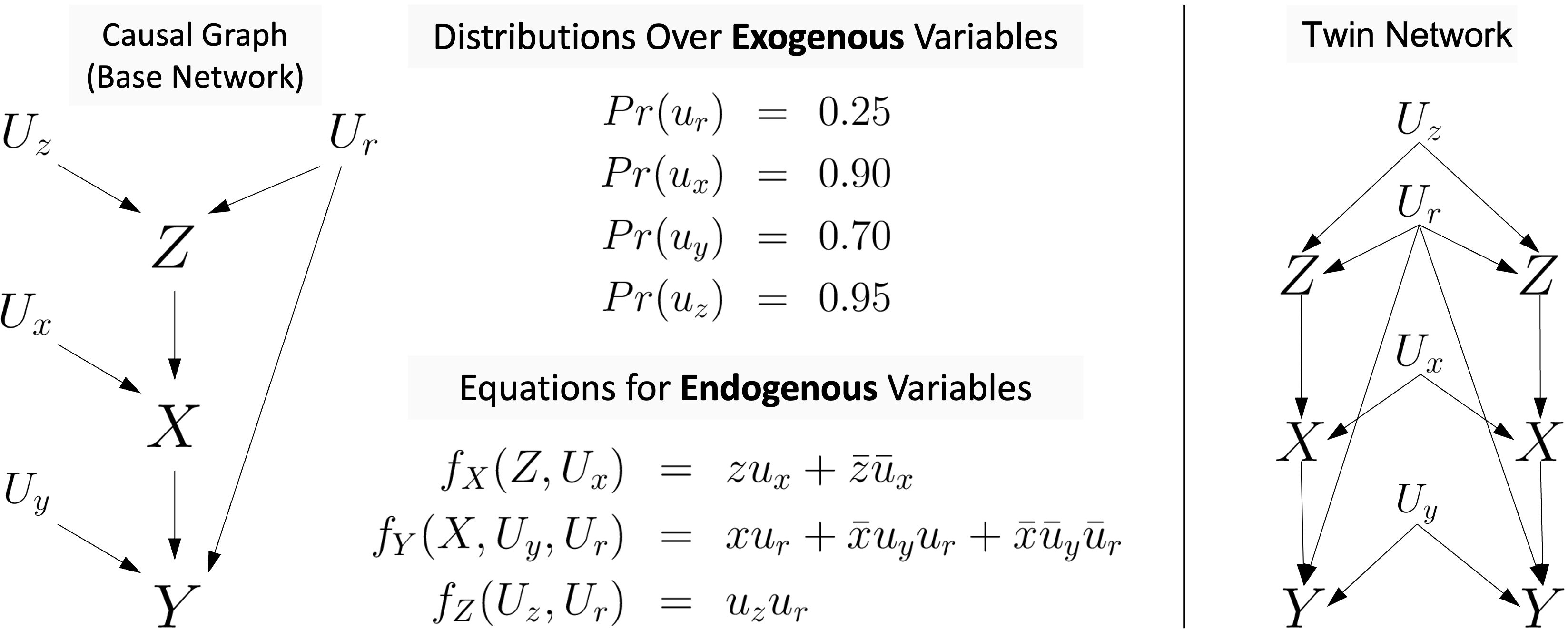
Figure 1: A structural causal model Bareinboim et al. (2021) and its twin network. Endogenous variables represent treatment ($X$), the outcome of ($Y$), and the presence of ($Z$), hypertension. Exogenous variables represent natural resistance to disease ($U_{r}$) and sources of variation affecting endogenous variables ($U_{x},U_{y},U_{z}$).

Counterfactual reasoning has received much interest as it inspires both introspection and contemplating scenarios that have not been seen before, and is therefore viewed by many as a hallmark of human intelligence. Figure 1 depicts a functional Bayesian network, also known as a structural causal model (SCM) Galles and Pearl (1998); Halpern (2000), which can be used to answer counterfactual queries. Variables without causes are called exogenous or root and variables with causes are called endogenous or internal. The only uncertainty in SCMs concerns the states of exogenous variables and this uncertainty is quantified using distributions over these variables. Endogenous variables are assumed to be functional: they are functionally determined by their causes where the functional relationships, also known as causal mechanisms, are specified by structural equations. These equations and the distributions over exogenous variables define the parameters of the causal graph, leading to a fully specified SCM which can be used to evaluate associational, interventional and counterfactual queries. For example, the SCM in Figure 1 has enough information to evaluate the counterfactual query ${\it Pr}(y_{x}|{\bar{x}},{\bar{y}})$: the probability that a patient who did not take the treatment and died would have been alive had they been given the treatment ($2.17\%$). A causal Bayesian network contains less information than a functional one (SCM) as it does not require endogenous variables to be functional, but it is sufficient to compute associational and interventional probabilities. A Bayesian network contains even less information as it does not require network edges to have a causal interpretation, only that the conditional independences encoded by the network are correct, so it can only compute associational probabilities.

All three forms of reasoning (and models) involve a directed acyclic graph (DAG) which we call the base network; see left of Figure 1. Associational and interventional reasoning can be implemented by applying classical inference algorithms to the base network. The time complexity can be bounded by $n\cdot\exp(w)$, where $n$ is the number of network nodes and $w$ is its treewidth (a graph-theoretic measure of connectivity). Counterfactual reasoning is more sophisticated and is based on a three-step process that involves abduction, intervention and prediction Balke and Pearl (1994b). When contemplating two worlds, this process can be implemented by applying classical inference algorithms to a twin network Balke and Pearl (1994b), obtained by duplicating endogenous nodes in the base network; see right of Figure 1. To compute the counterfactual query ${\it Pr}(y_{x}|{\bar{y}},{\bar{x}})$, one asserts ${\bar{y}},{\bar{x}}$ as an observation on one side of the twin network (real world) and computes the interventional query ${\it Pr}(y_{x})$ on the other side of the network (imaginary world). The time complexity can be bounded by $n^{t}\cdot\exp(w^{t})$, where $n^{t}$ is the number of nodes in the twin network and $w^{t}$ is its treewidth. A recent result provides a much tighter bound using the notion of causal treewidth Chen and Darwiche (2022); Darwiche (2021), which is no greater than treewidth but applies only when certain nodes in the base network are functional — in SCMs every endogenous node is functional.

One would expect the more sophisticated counterfactual reasoning with twin networks to be more expensive than associational/interventional reasoning with base networks since the former networks are larger and have more complex topologies. But the question is: How much more expensive? For example, can counterfactual reasoning be intractable on a twin network when associational/interventional reasoning is tractable on its base network? We address this question in the context of reasoning algorithms whose complexity is exponential only in the (causal) treewidth, such as the jointree algorithm Lauritzen and Spiegelhalter (1988), the variable elimination algorithm Zhang and Poole (1994); Dechter (1996) and circuit-based algorithms Darwiche (2003, 2022). In particular, we show in Sections 3 & 4 that the (causal) treewidth of a twin network is at most twice the (causal) treewidth of its base network plus one. Hence, the complexity of counterfactual reasoning on fully specified SCMs is no more than quadratic in the complexity of associational and interventional reasoning, so the former must be tractable if the latter is tractable. We extend our results in Section 5 to counterfactual reasoning that requires contemplating more than two worlds, where we also discuss a class of applications that require this type of reasoning and for which fully specified SCMs can be readily available. Our results apply directly to counterfactual reasoning on fully specified SCMs but we also discuss in Section 6 how they can sometimes be used in the context of counterfactual reasoning on data and a partially specified SCM. We finally present empirical results in Section 7 which reveal that, on average, the complexity gap between counterfactual and associational/interventional reasoning on fully specified SCMs can be smaller than what our worst-case bounds may suggest.

2 Technical Preliminaries

We next review the notions of treewidth Robertson and Seymour (1986) and causal treewidth Chen and Darwiche (2022); Darwiche (2021, 2020) which we use to characterize the computational complexity of counterfactual reasoning on fully specified SCMs. We also review the notions of elimination orders, jointrees and thinned jointrees which are the basis for defining (causal) treewidth and act as data structures that characterize the computational complexity of various reasoning algorithms. We use these notions extensively when stating and proving our results (proofs of all results are in Appendix A). We assume all variables are discrete. A variable is denoted by an uppercase letter (e.g. $X$) and its values by a lowercase letter (e.g. $x$). A set of variables is denoted by a bold uppercase letter (e.g. ${\mathbf{X}}$) and its instantiations by a bold lowercase letter (e.g. ${\mathbf{x}}$).

2.1 Elimination Orders and Treewidth

These are total orders of the network variables which drive, and characterize the complexity of, the classical variable elimination algorithm when computing associational, interventional and counterfactual queries. Consider a DAG $G$ where every node represents a variable. An elimination order $\pi$ for $G$ is a total ordering of the variables in $G$, where $\pi(i)$ is the $i^{th}$ variable in the order, starting from $i=1$. An elimination order defines an elimination process on the moral graph of DAG $G$ which is used to define the treewidth of $G$. The moral graph $G_{m}$ is obtained from $G$ by adding an undirected edge between every pair of common parents and then removing directions from all directed edges. When we eliminate variable $\pi(i)$ from $G_{m}$, we connect every pair of neighbors of $\pi(i)$ in $G_{m}$ and remove $\pi(i)$ from $G_{m}$. This elimination process induces a cluster sequence ${\mathbf{C}}_{1},{\mathbf{C}}_{2},\dots,{\mathbf{C}}_{n}$, where ${\mathbf{C}}_{i}$ is $\pi(i)$ and its neighbors in $G_{m}$ just before eliminating $\pi(i)$. The width of an elimination order is the size of its largest induced cluster minus $1$. The treewidth for DAG $G$ is the minimum width of any elimination order for $G$. The variable elimination algorithm computes queries in $O(n\cdot\exp(w))$ time where $n$ is the number of nodes in the (base or twin) network and $w$ is the width of a corresponding elimination order. Elimination orders are usually constructed using heuristics that aim to minimize their width. We use the popular minfill heuristic Kjaerulff (1990) in our experiments while noting that more effective heuristics may exist as shown in Kjærulff (1994); Larrañaga et al. (1997).

(a) DAG

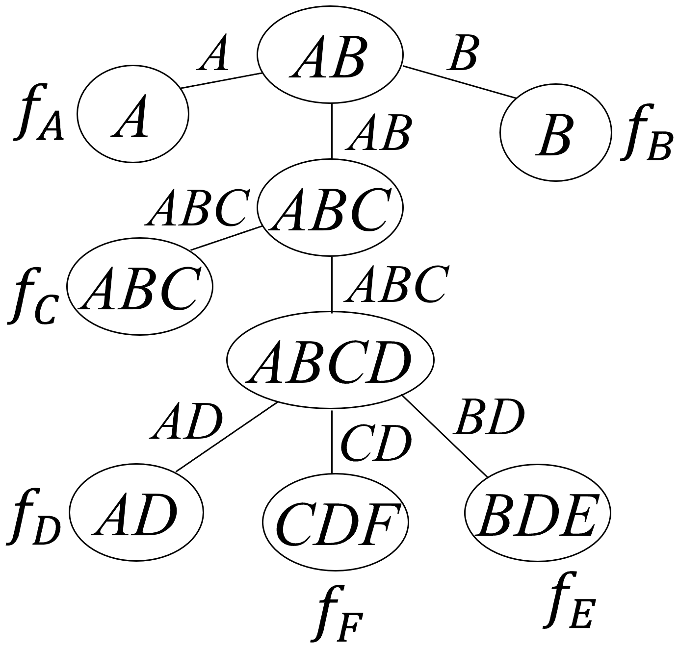
(b) jointree (width $3$)

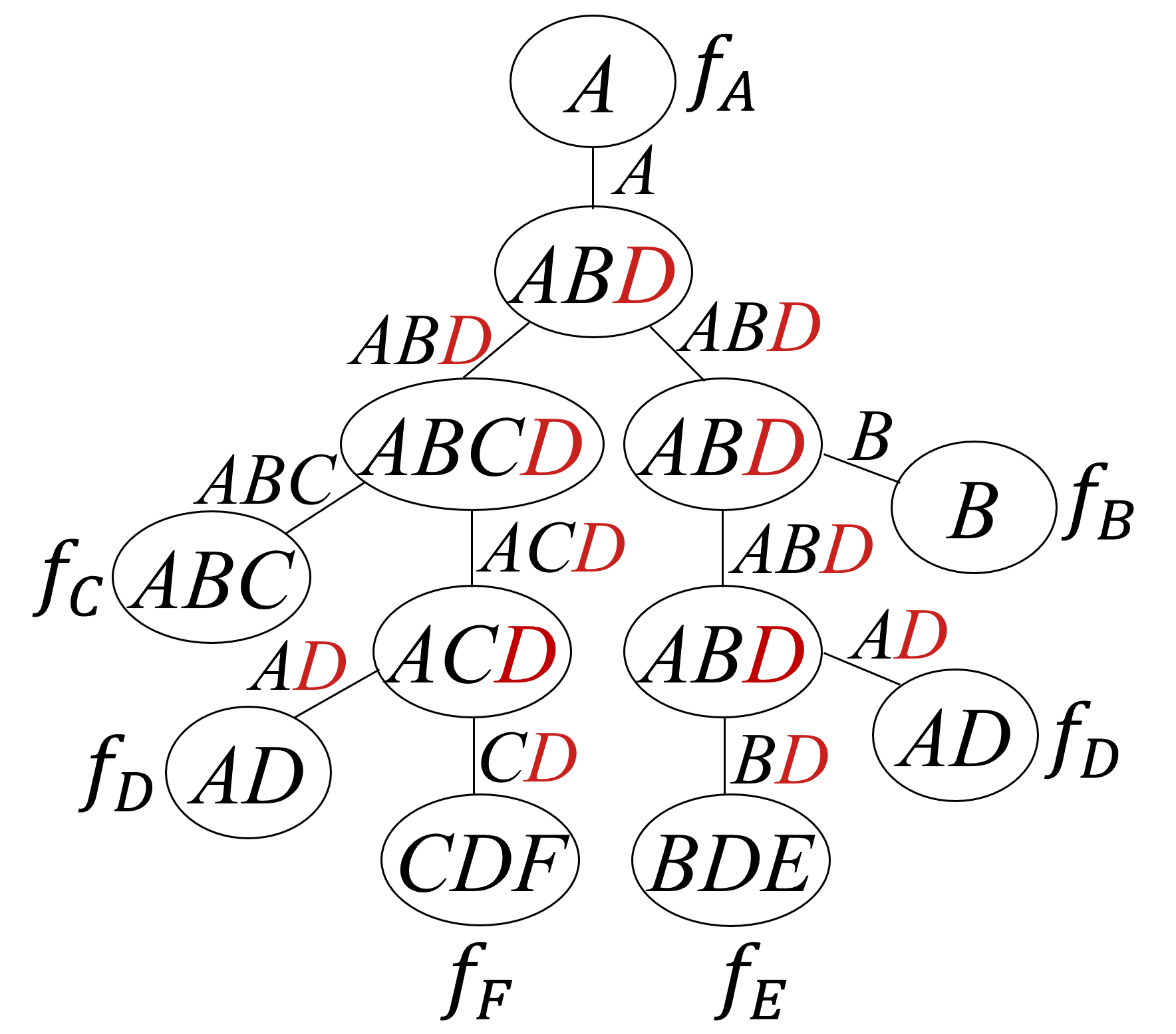
(c) thinned jointree (width $2$)

Figure 2: A family $f$ appears next to a jointree node $i$ iff $f$ is hosted by $i$ ($i\in{\cal H}(f)$). $D$ is functional and red variables are thinned.

(a) half adder

(b) base network

(c) twin network

(d) mutilated

Figure 3: Internal nodes in the base network (Figure (b)) are functional. Double-circled nodes have evidence.

2.2 Jointrees and Treewidth

These are data structures that drive, and characterize the complexity of, the classical jointree algorithm; see Figure 2(b). Let the family of variable $X$ in DAG $G$ be the set $f_{X}$ containing $X$ and its parents in $G$. A jointree for DAG $G$ is a pair ${\langle{\cal T},{\cal H}\rangle}$ where ${\cal T}$ is a tree and ${\cal H}$ is a function that maps each family $f$ of $G$ into nodes ${\cal H}(f)$ in ${\cal T}$ called the hosts of family $f$. The requirements are: only nodes with a single neighbor (called leaves) can be hosts; each leaf node hosts exactly one family; and each family must be hosted by at least one node. This induces a cluster ${\mathbf{C}}_{i}$ for each jointree node $i$ and a separator ${\mathbf{S}}_{ij}$ for each jointree edge $(i,j)$ which are defined as follows. Separator ${\mathbf{S}}_{ij}$ is the set of variables hosted at both sides of edge $(i,j)$. If jointree node $i$ is a leaf then cluster ${\mathbf{C}}_{i}$ is the family hosted by $i$; otherwise, ${\mathbf{C}}_{i}$ is the union of separators adjacent to node $i$. The width of a jointree is the size of its largest cluster minus $1$. The minimum width attained by any jointree for $G$ corresponds to the treewidth of $G$. The jointree algorithm computes queries in $O(n\cdot\exp(w))$ time where $n$ is the number of nodes and $w$ is the width of a corresponding jointree. Jointrees are usually constructed from elimination orders, and there are polytime, width-preserving transformations between elimination orders and jointrees; see (Darwiche, 2009, Ch 9) for details.

2.3 Thinned Jointrees and Causal Treewidth

To thin a jointree is to remove some variables from its separators (and hence clusters, which are defined in terms of separators); see Figure 2(c). Thinning can reduce the jointree width quite significantly, leading to exponential savings in reasoning time. Thinning is possible only when some variables in the network are functional, even without knowing the specific functional relationships (i.e., structural equations). The causal treewidth is the minimum width for any thinned jointree. Causal treewidth is no greater than treewidth and the former can be bounded when the latter is not. While this notion can be applied broadly as in Darwiche (2020), it is particularly relevant to counterfactual reasoning since every internal node in an SCM is functional so the causal treewidth for SCMs can be much smaller than their treewidth. There are alternate definitions of thinned jointrees. The next definition is based on thinning rules Chen and Darwiche (2022).

A thinning rule removes a variable from a separator under certain conditions. There are two thinning rules which apply only to functional variables. The first rule removes variable $X$ from a separator ${\mathbf{S}}_{ij}$ if edge $(i,j)$ is on the path between two leaf nodes that host the family of $X$ and every separator on that path contains $X$. The second rule removes variable $X$ from a separator ${\mathbf{S}}_{ij}$ if no other separator ${\mathbf{S}}_{ik}$ contains $X$, or no other separator ${\mathbf{S}}_{kj}$ contains $X$. A thinned jointree is obtained by applying these rules to exhaustion. Figure 2 depicts an optimal, classical jointree and a thinned jointree for the same DAG (the latter has smaller width).

The effectiveness of thinning rules depends on the number of jointree nodes that host a family $f$, $|{\cal H}(f)|$, and the location of these nodes in the jointree. One can enable more thinnings by increasing the number of jointree nodes that host each family $f$. This process is called replication where $|{\cal H}(f)|$ is called the number of replicas for family $f$. Replication comes at the expense of increasing the number of jointree nodes so the definition of causal treewidth limits this growth by requiring the jointree size to be a polynomial in the number of nodes in the underlying DAG; see Chen and Darwiche (2022) for details.

3 The Treewidth of Twin Networks

Consider Figure 3(a) which depicts a 2-bit half adder. Suppose the binary inputs $A$ and $B$ are randomly sampled from some distribution and the gates may not be functioning properly. This circuit can be modeled using the network in Figure 3(b). Variables $A,B,S,C$ represent the inputs and outputs of the circuit; $X,Y$ represent the health of the XOR gate and the AND gate; and $U$ represents an unknown external random sampler that decides the state of inputs $A$ and $B$. Suppose that currently input $A$ is high, input $B$ is low, yet both outputs $C$ and $S$ are low which is an abnormal circuit behavior. We wish to know whether the half adder would still behave correctly when we turn both inputs $A$ and $B$ on. This question can be formulated using the following counterfactual query: $Pr((c,{\bar{s}})_{a,b}|a,{\bar{b}},{\bar{c}},{\bar{s}})$. This query can be answered using a twin network as shown in Figure 3(c), where each non-root variable $V$ has a duplicate $[V]$. The current evidence $a,{\bar{b}},{\bar{c}},{\bar{s}}$ is asserted on the variables $A,B,C,S$ representing the real world and the interventional query $Pr((c,{\bar{s}})_{a,b})$ is computed on the duplicate variables $[A],[B],[C],[S]$ representing the imaginary world. This is done by removing the edges incoming into the intervened upon variables $[A],[B]$, asserting evidence $[a],[b]$ and finally computing the probability of $[c],[{\bar{s}}]$ as shown in Figure 3(d); see Pearl (2009) for an elaborate discussion of these steps. This basically illustrates how a counterfactual query can be computed using algorithms for associational queries, like variable elimination, but on a mutilated twin network instead of the base network.

We next show that the treewidth of a twin network is at most twice the treewidth of its base network plus one, which allows us to relate the complexities of assocational, interventional and counterfactual reasoning on fully specified SCMs. We first recall the definition of twin networks as proposed by Balke and Pearl (1994b).

Definition 1.

Given a base network $G$, its twin network $G^{t}$ is constructed as follows. For each internal variable $X$ in $G$, add a new variable labeled $[X]$. For each parent $P$ of $X$, if $P$ is an internal variable, make $[P]$ a parent of $[X]$; otherwise, make $P$ a parent of $[X]$. We will call $X$ a base variable and $[X]$ a duplicate variable.

For convenience, we use $[U]=U$ when $U$ is root. For variables ${\mathbf{X}}$, we use $[{\mathbf{X}}]$ to denote $\{[X]|X\in{\mathbf{X}}\}$. Figure 3(c) depicts the twin network for the base network in Figure 3(b).

3.1 Twin elimination orders

Our result on the treewidth of twin networks is based on converting every elimination order for the base network into an elimination order for its twin network while providing a guarantee on the width of the latter in terms of the width of the former. We provide a similar result for jointrees that we use when discussing the causal treewidth of twin networks.

Definition 2.

Consider an elimination order $\pi$ for a base network $G$. The twin elimination order $\pi^{t}$ is an elimination order for its twin network $G^{t}$ constructed by replacing each non-root variable $X$ in $\pi$ by $X,[X]$.

Consider the base network in Figure 3(b) and its elimination order $\pi=A$, $B$, $X$, $Y$, $S$, $C$, $U$. The twin elimination order will be $\pi^{t}=A$, $[A]$, $B$, $[B]$, $X$, $Y$, $S$, $[S]$, $C$, $[C]$, $U$. Recall that eliminating variables $\pi(i),\ldots,\pi(n)$ from a base network $G$ induces a cluster sequence ${\mathbf{C}}_{1},\ldots,{\mathbf{C}}_{n}$. We use ${\mathbf{C}}(X)$ to denote the cluster of eliminated variable $X$. Similarly, eliminating variables from a twin network $G^{t}$ induces a cluster sequence and we use ${\mathbf{C}}^{t}(X)$ to denote the cluster of eliminated variable $X$ and ${\mathbf{C}}^{t}([X])$ to denote the cluster of its eliminated duplicate $[X]$.

Theorem 1.

Suppose we are eliminating variables from base network $G$ using an elimination order $\pi$ and eliminating variables from its twin network $G^{t}$ using the twin elimination order $\pi^{t}$. For every variable $X$ in $G$, we have ${\mathbf{C}}^{t}(X)\subseteq{\mathbf{C}}(X)\cup[{\mathbf{C}}(X)]$ and ${\mathbf{C}}^{t}([X])\subseteq{\mathbf{C}}(X)\cup[{\mathbf{C}}(X)]$.

This theorem has two key corollaries. The first relates the widths of an elimination order and its twin elimination order.

Corollary 1.

Let $w$ be the width of elimination order $\pi$ for base network $G$ and let $w^{t}$ be the width of twin elimination order $\pi^{t}$ for twin network $G^{t}$. We then have $w^{t}\leq 2w+1$.

The above bound is tight as shown in Appendix B. The next corollary gives us our first major result.

Corollary 2.

If $w$ is the treewidth of base network $G$ and $w^{t}$ is the treewidth of its twin network $G^{t}$, then $w^{t}\leq 2w+1$.

3.2 Twin jointrees

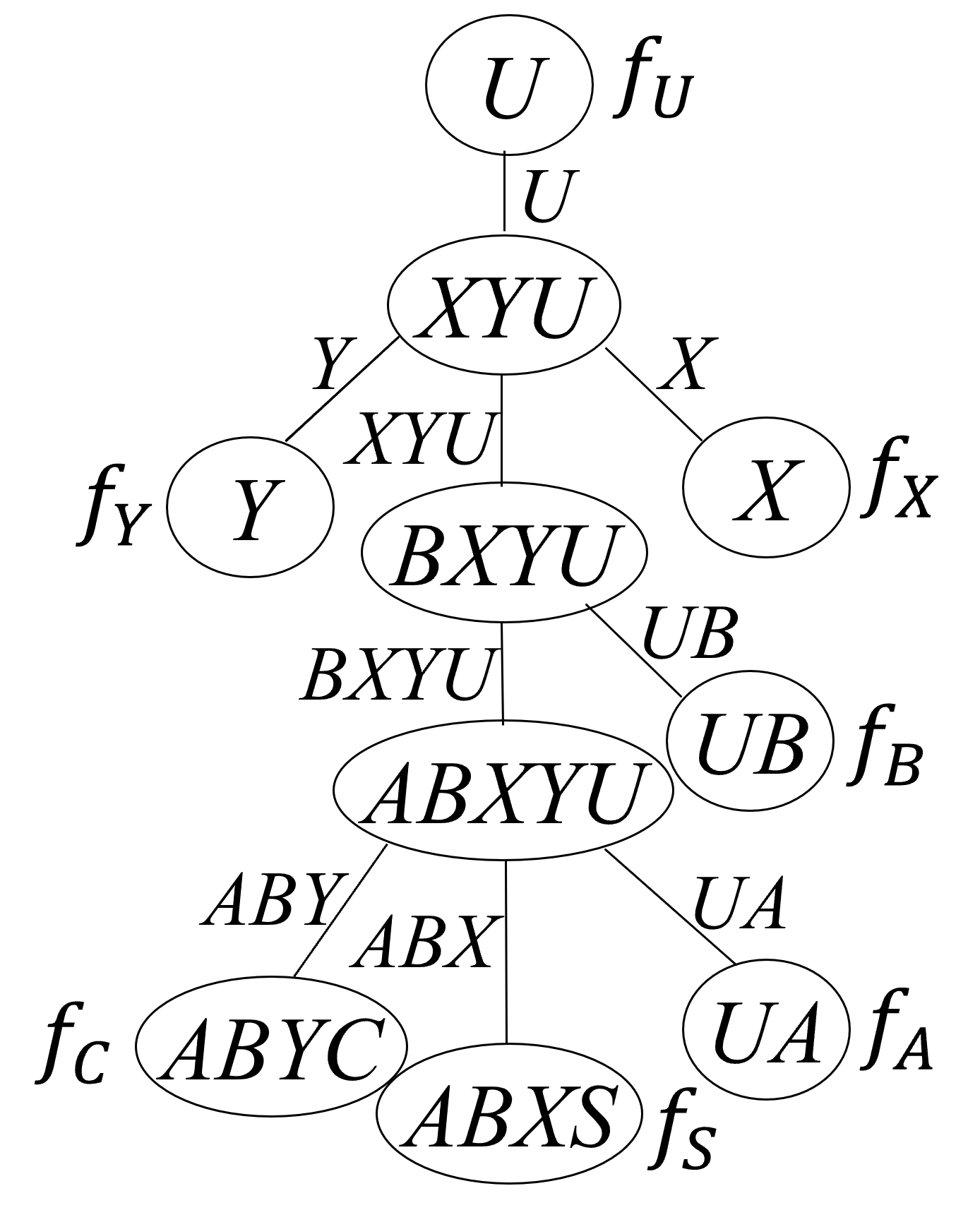
(a) base jointree

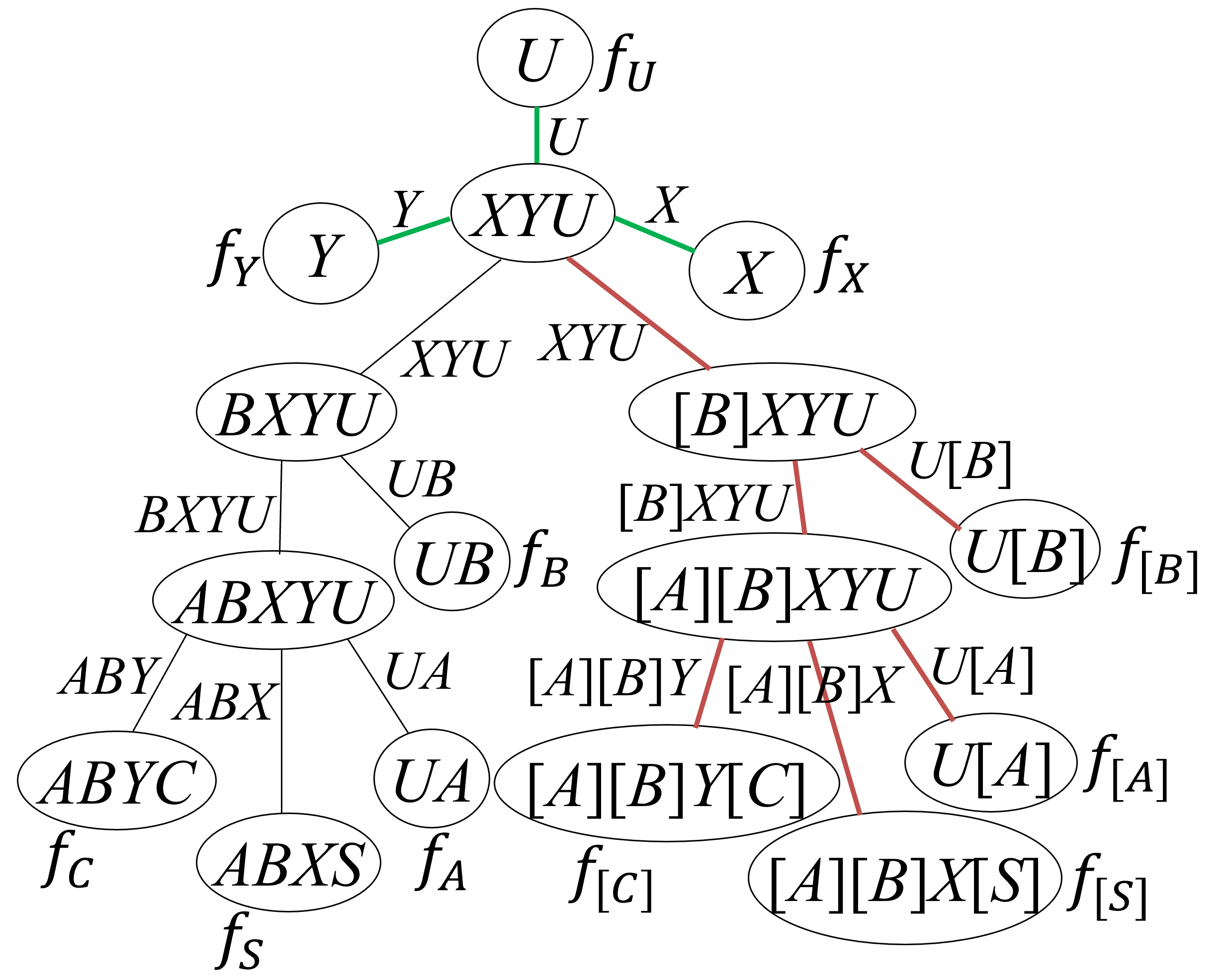
(b) twin jointree using Algorithm 1

Figure 4: A family $f$ appears next to a jointree node $i$ iff the family is hosted by that node ($i\in{\cal H}(f)$).

We will now provide a similar result for jointrees. That is, we will show how to convert a jointree ${\langle{\cal T},{\cal H}\rangle}$ for a base network $G$ into a jointree ${\langle{\cal T}^{t},{\cal H}^{t}\rangle}$ for its twin network $G^{t}$ while providing a guarantee on the width/size of the twin jointree in terms of the width/size of the base jointree. This may seem like a redundant result given Corollary 1 but the provided conversion will actually be critical for our later result on bounding the causal treewidth of twin networks. It can also be significantly more efficient than constructing a jointree by operating on the (larger) twin network.

Our conversion process operates on a jointree after directing its edges away from some node $r$, call it a root. This defines a single parent for each jointree node $i\neq r$, which is the neighbor of $i$ closest to root $r$, with all other neighbors of $i$ being its children. These parent-child relationships are invariant when running the algorithm. We also use a subroutine for duplicating the jointree nodes rooted at some node $i$. This subroutine duplicates node $i$ and its descendant while also duplicating the edges connecting these nodes. If a duplicated node $j$ hosts a family $f$, this subroutine will make $[j]$ host the duplicate family $[f]$ (so $j\in{\cal H}(f)$ iff $[j]\in{\cal H}([f])$).

Algorithm 1 Jointree to Twin Jointree

1:procedure Make-Twin-Jointree(${\langle{\cal T},{\cal H}\rangle},r,p$)

2:    $\Sigma\leftarrow$ leaf nodes at or below node $r$

3:    if nodes in $\Sigma$ only host families for root variables then

4:         return     

5:    if nodes in $\Sigma$ only host families for internal variables then

6:         duplicate the jointree nodes rooted at node $r$

7:         add $[r]$ as a child of $p$

8:    else

9:         for each child $k$ of node $r$ do

10:             $\textsc{Make-Twin-Jointree}({\langle{\cal T},{\cal H}\rangle},k,r)$              

The conversion process is given in Algorithm 1 which should be called initially with a root $r$ that does not host a family for an internal DAG node and $p=null$. The twin jointree in Figure 4(b) was obtained from the base jointree in Figure 4(a) by this algorithm which simply adds nodes and edges to the base jointree. If an edge $(i,j)$ in the base jointree is duplicated by Algorithm 1, we call $(i,j)$ a duplicated edge and $([i],[j])$ a duplicate edge. Otherwise, we call $(i,j)$ an invariant edge. In Figure 4(b), duplicate edges are shown in red and invariant edges are shown in green. We now have the following key result on these twin jointrees.

Theorem 2.

If the input jointree to Alg. 1 has separators ${\mathbf{S}}$ and the output jointree has separators ${\mathbf{S}}^{t}$, then for duplicated edges $(i,j)$, ${\mathbf{S}}^{t}_{ij}={\mathbf{S}}_{ij}$; for duplicate edges $([i],[j])$, ${\mathbf{S}}^{t}_{[i][j]}=[{\mathbf{S}}_{ij}]$; and for invariant edges $(i,j)$, ${\mathbf{S}}^{t}_{ij}={\mathbf{S}}_{ij}\cup[{\mathbf{S}}_{ij}]$.

One can verify that the separators in Figure 4 satisfy these properties. The following result bounds the width and size of twin jointrees generated by Algorithm 1.

Corollary 3.

Let $w$ be the width of a jointree for base network $G$ and let $n$ be the number of jointree nodes. Calling Algorithm 1 on this jointree will generate a jointree for twin network $G^{t}$ whose width is no greater than $2w+1$ and whose number of nodes is no greater than $2n$.

The above bound on width is tight as shown in Appendix B. Since treewidth can be defined in terms of jointree width, the above result leads to the same guarantee of Corollary 2 on the treewidth of twin networks. However, the main role of the construction in this section is in bounding the causal treewidth of twin networks. This is discussed next.

4 The Causal Treewidth of Twin Networks

Recall that causal treewidth is a more refined notion than treewidth as it uses more information about the network. In particular, this notion is relevant when we know that some variables in the network are functional, without needing to know the specific functions (equations) of these variables. By exploiting this information, one can construct thinned jointrees that have smaller separators and clusters compared to classical jointrees, which can lead to exponential savings in reasoning time Chen and Darwiche (2022); Darwiche (2021, 2020). As mentioned earlier, the causal treewidth corresponds to the minimum width of any thinned jointree. This is guaranteed to be no greater than treewidth and can be bounded when treewidth is not Darwiche (2021). We next show that the causal treewidth of a twin network is also at most twice the causal treewidth of its base network plus one.

Theorem 3.

Consider a twin jointree constructed by Algorithm 1 from a base jointree with thinned separators ${\mathbf{S}}$. The following are valid thinned separators for this twin jointree: for duplicated edges $(i,j)$, ${\mathbf{S}}^{t}_{ij}={\mathbf{S}}_{ij}$; for duplicate edges $([i],[j])$; ${\mathbf{S}}^{t}_{[i][j]}=[{\mathbf{S}}_{ij}]$; and for invariant edges $(i,j)$, ${\mathbf{S}}^{t}_{ij}={\mathbf{S}}_{ij}\cup[{\mathbf{S}}_{ij}]$.

This theorem shows that a thinned, base jointree can be easily converted into a thinned, twin jointree. This is significant for two reasons. First, this method avoids the explicit construction of thinned jointrees for twin networks which can be quite expensive computationally Chen and Darwiche (2022). Second, we have the following guarantee on the width of thinned, twin jointrees constructed by Theorem 3.

Corollary 4.

Consider the thinned, base and twin jointrees in Theorem 3. If the thinned, base jointree has width $w$, then the thinned, twin jointree has width no greater than $2w+1$.

Due to space constraints, we include a thinned jointree for the base network and the corresponding thinned, twin jointree constructed by Algorithm 1 and Theorem 3 in Appendix C. We can now bound the causal treewidth of twin networks.

Corollary 5.

If $w$ and $w^{t}$ are the causal treewidths of a base network and its twin network, then $w^{t}\leq 2w+1$.

5 Counterfactual Reasoning Beyond Two Worlds

Figure 5: A base network and its 3-world network.

Standard counterfactual reasoning contemplates two worlds, one real and another imaginary, while assuming that exogenous variables correspond to causal mechanisms that govern both worlds. This motivates the notion of a twin network as it ensures that these causal mechanisms are invariant. We can think of counterfactual reasoning as a kind of temporal reasoning where endogenous variables can change their states over time. A more general setup arises when we allow some exogenous variables to change their states over time. For example, consider again the half adder in Figure 3(a) and its base network in Figure 5. Suppose we set inputs $A$ and $B$ to high and low and observe outputs $S$ and $C$ to be high and low, which is a normal behavior. We then set both inputs to low and observe that the outputs do not change, which is an abnormal behavior. We then aim to predict the state of outputs if we were to set both inputs to high. This scenario involves three time steps (worlds). Moreover, while the health of gates $X$ and $Y$ are invariant over time, we do not wish to make the same assumption about the inputs $A$ and $B$. We can model this situation using the network in Figure 5, which is a more general type of networks that we call $N$-world networks.

Definition 3.

Consider a base network $G$ and let ${\mathbf{R}}$ be a subset of its roots and $N\geq 1$ be an integer. The $N$-world network $G^{N}$ of $G$ is constructed as follows. For each variable $X$ in $G$ that is not in ${\mathbf{R}}$, replace it with N duplicates of $X$, labeled ${X}^{1},{X}^{2},\dots,{X}^{N}$. For each parent $P$ of $X$, if $P$ is in ${\mathbf{R}}$, make $P$ a parent of ${X}^{i}$ for all $i\in 1,2,\dots,N$. Otherwise, make ${P}^{i}$ a parent of ${X}^{i}$ for all $i\in 1,2,\dots,N$.

This definition corresponds to the notion of a parallel worlds model Avin et al. (2005) when ${\mathbf{R}}$ contains all roots in the base network. Moreover, twin networks fall as a special case when $N=2$ and ${\mathbf{R}}$ contains all roots of the base network. We next bound the (causal) treewidth of $N$-world networks by the (causal) treewidth of their base networks.

Theorem 4.

If $w$ and $w^{t}$ are the (causal) treewidths of a base network and its $N$-world network, then $w^{t}\leq N(w+1)-1$.

The class of $N$-world networks is a subclass of dynamic Bayesian networks Dean and Kanazawa (1989) and is significant for a number of reasons. First, as illustrated above, it arises when reasoning about the behavior of systems consisting of function blocks (e.g., gates) Hamscher et al. (1992). These kinds of physical systems can be easily modeled using fully specified SCMs, where the structural equations correspond to component behaviors and the distributions over exogenous variables correspond to component reliabilities; see (Darwiche, 2009, Ch 5) for a textbook discussion and Mengshoel et al. (2010) for a case study of a real-world electrical power system. More broadly, $N$-world networks allow counterfactual reasoning that involves conflicting observations and actions that arise in multiple worlds as in the unit selection problem Li and Pearl (2022)—for example, Huang and Darwiche (2023) used Theorem 4 to obtain bounds on the complexity of this problem. See also Avin et al. (2005); Shpitser and Pearl (2007, 2008) for further applications of $N$-world networks in the context of counterfactual reasoning. Appendix D shows that the treewidth bound of Theorem 4 holds for a generalization of $N$-world networks that permits the duplication of only a subset of base nodes and allows certain edges that extend between worlds.

Our complexity bounds thus far apply to any counterfactual query. For a specific counterfactual query, we can further reduce the complexity of inference by pruning nodes and edges as in (Darwiche, 2009, Ch 6) and merging nodes which leads to counterfactual graphs as in Shpitser and Pearl (2007).

6 Counterfactual Reasoning with Partially Specified SCMs

The results we presented on $N$-world networks, which include twin networks, apply directly to fully specified SCMs. In particular, in the context of variable elimination and jointree algorithms, these results allow us to bound the complexity of computing counterfactual queries in terms of the complexity of computing associational/interventional queries. Moreover, they provide efficient methods for constructing elimination orders and jointrees that can be used for computing counterfactual queries based on the ones used for answering associational/interventional queries, while ensuring that the stated bounds will be realized. Recall again that our bounds and constructions apply to both traditional treewidth and the more recent causal treewidth.

Causal reasoning can also be conducted on partially specified SCMs and data, which is a more common and challenging task. A partially specified SCM typically includes the SCM structure and some information about its parameters (i.e., its structural equations and the distributions over its exogenous variables). For example, we may not know any of the SCM paramaters, or we may know the structural equations but not the distributions over exogenous variables as assumed in Zaffalon et al. (2021). A central question in this setup is whether the available information, which includes data, is sufficient to obtain a point estimate for the causal query of interest, in which case the query is said to be identifiable. A significant amount of work has focused on characterizing conditions under which causal queries (both counterfactual and interventional) are identifiable; see, Pearl (2009); Spirtes et al. (2000) for textbook discussions of this subject and Shpitser and Pearl (2008); Correa et al. (2021) for some results on the identification of counterfactual queries.

When a query is identifiable, the classical approach for estimating it is to derive an estimand using techniques such as the do-calculus for interventional queries Pearl (1995); Tian and Pearl (2002); Shpitser and Pearl (2006). Some recent approaches take a different direction by first estimating the SCM parameters to yield a fully specified SCM that is then used to answer (identifiable) interventional and counterfactual queries using classical inference algorithms Zaffalon et al. (2022, 2021); Darwiche (2021). Our results on twin and $N$-world networks apply directly in this case as they can be used when conducting inference on the fully parameterized SCM. For unidentifiable queries, the classical approach is to derive a closed-form bound on the query; see, for example, Balke and Pearl (1994a); Pearl (1999); Tian and Pearl (2000); Dawid et al. (2017); Rosset et al. (2018); Evans (2018); Zhang et al. (2021); Mueller et al. (2022). Some recent approaches take a different direction for establishing bounds, such as reducing the problem into one of polynomial programming Duarte et al. (2021); Zhang et al. (2022) or inference on credal networks Zaffalon et al. (2020); Cozman (2000); Mauá and Cozman (2020). Another recent direction is to establish (approximate) bounds by estimating SCM parameters and then using classical inference algorithms on the fully specified SCM to obtain point estimates Zaffalon et al. (2021, 2022). Since the query is not identifiable, different parametrizations can lead to different point estimates which are employed to improve (widen) the computed bounds. Our results can also be used in this case for computing point estimates based on a particular parametrization (fully specified SCM) within the overall process of establishing bounds.

7 Experimental Results

We consider experiments that target random networks whose structures emulate the structures of SCMs used in counterfactual reasoning. We have a few objectives in mind. First, we wish to compare the widths of base and twin jointrees, with and without thinning. These widths do not correspond to (causal) treewidth since the jointrees are constructed using heuristics (finding optimal jointrees is NP-hard). Next, we want to compare the quality of twin jointrees constructed by Algorithm 1 (TWIN-ALG1), which operates directly on a base jointree, to the quality of twin jointrees obtained by applying the minfill heuristic to a twin network (TWIN-MF). Recall that the former method is more efficient than the latter method. Finally, we wish to conduct a similar comparison between the thinned, twin jointrees constructed according to Theorem 3 (TWIN-THM3) and the thinned, twin jointrees obtained by applying the minfill heuristic and thinning rules to a twin network (TWIN-MF-RLS). Again, the former method is more efficient than the latter. The widths of these jointrees will be compared to the widths of base jointrees constructed by minfill (BASE-MF) and thinned, base jointrees constructed by minfill and thinning rules (BASE-MF-RLS).

We generated random networks according to the method used in Darwiche (2020). Given a number of nodes $n$ and a maximum number of parents $p$, the method chooses the parents of node $X_{i}$ randomly from the set $X_{1},\ldots,X_{i-1}$. The number of parents for node $X_{i}$ is chosen randomly from the set $0,\ldots,min(p,i-1)$. We refer to these networks as rNET. We then consider each internal node $N$ and add a unique root $R$ as parent for $N$. This is meant to emulate the structure of SCMs as the exogenous variable $R$ can be viewed as representing the different causal mechanisms for endogenous variable $N$. We refer to these modified networks as rSCM. The twin networks of rSCM are more complex than those for rNET since more variables are shared between the two slices representing the real and imaginary worlds (i.e., more information is shared between the two worlds). We used $n\in\{50,75,100,125,150,200,250,300\}$ and $p\in\{3,5,7\}$. For each combination of $n$ and $p$, we generated $50$ random, base networks and reported averages of two properties for the constructed jointrees: width and normalized width. If a jointree has clusters ${\mathbf{C}}_{1},\ldots,{\mathbf{C}}_{n}$, then normalized width is $\log_{2}\sum_{i=1}^{n}2^{|{\mathbf{C}}_{i}|}$. This accounts for all clusters in the jointree (instead of just the largest one) and the jointree size. The data we generated occupies significant space so we included it in Appendix E while providing representative plots in Figure 6 for jointree widths under $p=5$. We next discuss patterns exhibited in these plots and the full data in Appendix E, which also includes experiments using random networks generated according to the method in Ide and Cozman (2002).

First, the widths of twin jointrees are always less than twice the widths of their base jointrees and often significantly less than that. This is not guaranteed by our theoretical bounds as those apply to (causal) treewidth not to the widths of jointrees produced by heuristics — the latter widths are an upper bound on the former. Second, constructing a twin jointree by directly applying Algorithm 1 to a base jointree (TWIN-ALG1) is relatively comparable to constructing the twin jointree by operating on the twin network (TWIN-MF), as would normally be done. This also holds for thinned jointrees (TWIN-THM3 vs TWIN-MF-RLS) and is encouraging since the former methods are much more efficient than the latter ones. Third, the employment of thinned jointrees can lead to significant reduction in width and hence an exponential reduction in reasoning time. This can be seen by comparing the widths of twin jointrees TWIN-THM3 and TWIN-ALG1 since the former is thinned but the latter is not (similarly for TWIN-MF-RLS and TWIN-MF). Fourth, the twin jointrees of rSCM have larger widths than those of rNET. Recall that in rSCM, every endogenous variable has its own exogenous variable as a parent. Therefore, the distribution over exogenous variables has a larger space in rSCM compared to rNET. Since this distribution needs to be shared between the real and imaginary worlds, counterfactual reasoning with rSCM is indeed expected to be more complex computationally than reasoning with rNET. Finally, consider Figure 6(b) for a bottom-line comparison between the complexity of counterfactual reasoning and the complexity of associational/interventional reasoning in practice. Jointrees BASE-MF have the smallest widths for base networks so these are the jointrees one would use for associational/interventional reasoning. The best twin jointrees are TWIN-MF-RLS which are thinned. This is what one would use for counterfactual reasoning. The widths of latter jointrees are always less than twice the widths of the former, and quite often significantly much less.

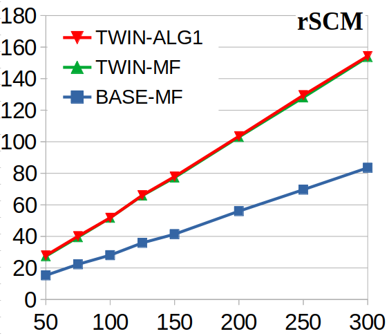
(a) classical jointrees

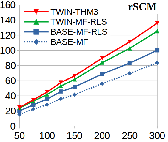
(b) thinned jointrees

Figure 6: Width of jointrees (y-axis) against number of base network nodes (x-axis) for maximum number of parents $p=5$.

8 Conclusion

We studied the complexity of counterfactual reasoning on fully specified SCMs in relation to the complexity of associational and interventional reasoning on these models. Our basic finding is that in the context of algorithms based on (causal) treewidth, the former complexity is no greater than quadratic in the latter when counterfactual reasoning involves only two worlds. We extended these results to counterfactual reasoning that requires multiple worlds, showing that the gap in complexity is bounded polynomially by the number of needed worlds. Our empirical results suggest that for two types of random SCMs, the complexity of counterfactual reasoning is closer to that of associational and interventional reasoning than our worst-case theoretical analysis may suggest. While our results directly target counterfactual reasoning on fully specified SCMs, we also discussed cases when they can be applied to counterfactual reasoning on partially specified SCMs that are coupled with data.

Appendix A Proofs

Proof of Theorem 1

Consider a base network $G$ and its twin network $G^{t}$. We first introduce a set notation $\{X,[X]\}$, which contains both the base and duplicate variable for $X$ if $X$ is an internal variable and collapses to a single variable if $X$ is a root variable.

For an elimination order $\pi$ on a base network $G$, Darwiche [2009] defines a graph sequence $G_{1},G_{2},\dots,G_{n}$ induced by $\pi$, where $G_{1}$ is the moral graph for $G$, and $G_{i+1}$ is the result of eliminating $\pi(i)$ from $G_{i}$. Similarly, we define a twin graph sequence $G^{t}_{1},G^{t}_{2},\dots,G^{t}_{n}$, where $G^{t}_{1}$ is the moral graph for $G^{t}$, and $G^{t}_{i+1}$ is the result of eliminating $\{\pi(i),[\pi(i)]\}$ from $G^{t}_{i}$.

Consider $G_{i}$ in the graph sequence induced by $\pi$ on $G$. For each variable $X$ in $G_{i}$, let $G_{i}(X)$ be the set consisting of $X$ and its neighbors in $G_{i}$. Similarly, let $G^{t}_{i}(X)$ and $G^{t}_{i}([X])$ denote the set consisting of $X$ and its neighbors, and the set consisting of $[X]$ and its neighbors in $G^{t}_{i}$, respectively. By definition, $G_{i}(\pi(i))={\mathbf{C}}(\pi(i))$ and $G^{t}_{i}(\pi(i))={\mathbf{C}}^{t}(\pi(i))$.

We first propose a Lemma that relates $G^{t}_{i}(X)$ and $G_{i}(X)$.

Lemma 1.

Suppose we apply elimination order $\pi$ to a base network $G$ and apply $\pi^{t}$ to its twin network $G^{t}$. Then for each variable $X$ in $G_{i}$, we have $G^{t}_{i}(X)\subseteq G_{i}(X)\cup[G_{i}(X)]$ and $G^{t}_{i}([X])\subseteq G_{i}(X)\cup[G_{i}(X)]$.

Proof.

We will prove this by induction on $G^{t}_{i}$. The statement holds initially for $G^{t}_{1}$ by the definition of twin networks. Suppose the statement holds for $G^{t}_{i-1}$, i.e. $G^{t}_{i-1}(X)\subseteq G_{i-1}(X)\cup[G_{i-1}(X)]$ and $G^{t}_{i-1}([X])\subseteq G_{i-1}(X)\cup[G_{i-1}(X)]$ for every $\{X,[X]\}$ in $G^{t}_{i-1}$, we need to show the statement holds for $G^{t}_{i}$.

For simplicity, let $Y$ denote the variable being eliminated at step $i$, i.e. $Y=\pi(i-1)$. WLG, consider each base variable $X$ in $G^{t}_{i}$ (similar argument can be applied to each duplicate variable $[X]$). $G^{t}_{i}(X)$ is affected by the elimination of $\{Y,[Y]\}$ iff $X$ is a neighbor of $\{Y,[Y]\}$ in $G^{t}_{i-1}$. Moreover, by induction, $X$ is a neighbor of $\{Y,[Y]\}$ in $G^{t}_{i-1}$ only if $X$ is a neighbor of $Y$ in $G_{i-1}$.

When $X$ is not a neighbor of $Y$, then $G^{t}_{i}(X)=G^{t}_{i-1}(X)$ and $G_{i}(X)=G_{i-1}(X)$, so the statement holds.

When $X$ is a neighbor of $Y$, $G_{i}(X)=G_{i-1}(X)\cup G_{i-1}(Y)\setminus\{Y\}$ by the definition of variable elimination. We can then bound $G^{t}_{i}(X)$ as follows:

$$G^{t}_{i}(X) \subseteq (G^{t}_{i-1}(X)\cup G^{t}_{i-1}(Y)\cup G^{t}_{i-1}([Y]))\setminus\{Y,[Y]\}$$

(eliminating $$\{Y,[Y]\} G^{t}$$ on )

$$\subseteq (G_{i-1}(X)\cup[G_{i-1}(X)]\cup G_{i-1}(Y)\cup[G_{i-1}(Y)])\setminus\{Y,[Y]\}$$

(by inductive hypothesis)

$$= (G_{i-1}(X)\cup G_{i-1}(Y))\cup([G_{i-1}(X)]\cup[G_{i-1}(Y)])\setminus\{Y,[Y]\}$$

$$= G_{i}(X)\cup[G_{i}(X)].\qed$$

Proof of Theorem 1.

Consider each variable $X$ that is eliminated at step $i$, i.e. $X=\pi(i)$. By Lemma 1, ${\mathbf{C}}^{t}(X)=G^{t}_{i-1}(X)\subseteq G_{i-1}(X)\cup[G_{i-1}(X)]={\mathbf{C}}(X)\cup[{\mathbf{C}}(X)]$.

We next bound ${\mathbf{C}}^{t}([X])$ if $X$ is an internal variable,

$${{\mathbf{C}}^{t}}([X]) \subseteq (G^{t}_{i-1}([X])\cup{\mathbf{C}}^{t}(X))\setminus\{X\}$$

(eliminating $$X G^{t}_{i-1}$$ from )

$$\subseteq G_{i-1}(X)\cup[G_{i-1}(X)]\setminus\{X\}$$

(by Lemma 1)

$$\subseteq {\mathbf{C}}(X)\cup[{\mathbf{C}}(X)].\qed$$

Proof of Corollary 1.

By Theorem 1, for every base variable $X\in G^{t}$, $|{\mathbf{C}}^{t}(X)|\leq|{\mathbf{C}}(X)\cup[{\mathbf{C}}(X)]|\leq 2|{\mathbf{C}}(X)|$. Similarly, for every duplicate variable $[X]\in G^{t}$, $|{\mathbf{C}}^{t}([X])|\leq|{\mathbf{C}}(X)\cup[{\mathbf{C}}(X)]|\leq 2|{\mathbf{C}}(X)|$. So $w^{t}=\max_{X\in G^{t}}{|{\mathbf{C}}^{t}(X)|}-1\leq 2\max_{X\in G}{|{\mathbf{C}}(X)|}-1=2(w+1)-1=2w+1$. ∎

Proof of Corollary 2.

Consider an optimal elimination order $\pi$ for base network $G$ with width $w$. By Corollary 1, the twin elimination order for $G^{t}$ with width no more than $2w+1$. It follows that the treewidth of $G^{t}$ is no more than $2w+1$. ∎

Proof of Theorem 2

We first state a key observation from Algorithm 1, which is formulated as Lemma 2. For simplicity, we say a leaf node hosts variable $X$ if it hosts a family that contains $X$.

Lemma 2.

Consider each invariant edge $(i,j)$ in a twin jointree constructed from Algorithm 1. A variable $X$ is hosted in some leaf on the $i$-side of the edge iff $[X]$ is also hosted in some leaf on the $i$-side of the edge.

Proof.

If $X$ is a root variable, then $X=[X]$ and the lemma holds. Now suppose $X$ is an internal variable. Let $k$ be the leaf node on the $i$-side of the edge that hosts $X$, it suffices to show that $k$ is duplicated into a $[k]$ on the $i$-side that hosts $[X]$.

Since $X$ is an internal variable, $k$ hosts either the family for $X$ or a family for some child of $X$. In either case, $k$ hosts a family for an internal variable. Moreover, $k$ is contained in some subtree rooted at $u$ whose leaves host only families for internal variables. Since $k$ is on the $i$-side of the invariant edge $(i,j)$, $u$ is also on the $i$-side of the edge. Hence the duplicate leaf $[k]$, which hosts $[X]$, is also on the $i$-side of the edge.

Conversely, suppose $[X]$ is hosted by some leaf $[k]$ on the $i$-side of edge $(i,j)$, then $[k]$ hosts some family for a duplicate variable. $[k]$ is contained in some duplicate subtree rooted at $[u]$ whose leaves only host families for duplicate variables. It follows that the base subtree rooted at $u$ is located on the $i$-side of the edge and contains a base node $k$ hosting $X$. ∎

We first recall the definition of separators: $X\in{\mathbf{S}}_{ij}$ if and only if $X$ is hosted on both sides of the edge $(i,j)$. For simplicity, we use $\mathtt{vars}(i,j)$ to denote the variables that appear on the $i$-side of the edge $(i,j)$ in the base jointree. Similarly, we use $\mathtt{vars}^{t}(i,j)$ and to denote the variables that appear on the $i$-side in the twin jointree. By definition, for each edge $(i,j)$, ${\mathbf{S}}_{ij}=\mathtt{vars}(i,j)\cap\mathtt{vars}(j,i)$ and ${\mathbf{S}}^{t}_{ij}=\mathtt{vars}^{t}(i,j)\cap\mathtt{vars}^{t}(j,i)$. Given a jointree and its root, we say that a jointree node $j$ is above a jointree node $i$ if $j$ is closer to the root than $i$, and that $j$ is below $i$ if $j$ is further from the root than $i$.

Proof of Theorem 2.

We derive the separators for each type of edges. WLG, for each edge $(i,j)$, assume that $j$ is above $i$. First consider each duplicated edge $(i,j)$, we have $\mathtt{vars}^{t}(i,j)=\mathtt{vars}(i,j)$ by Algorithm 1. Moreover, $\mathtt{vars}^{t}(j,i)$ can only contain extra duplicate variables comparing to $\mathtt{vars}(j,i)$. Thus, ${\mathbf{S}}^{t}_{ij}={\mathbf{S}}_{ij}$.

For each duplicate edge $([i],[j])$, we have $\mathtt{vars}^{t}([i],[j])=[\mathtt{vars}(i,j)]$ by Algorithm 1. We next show that for each $[X]\in\mathtt{vars}^{t}([i],[j])$, $[X]\in\mathtt{vars}^{t}([j],[i])$ iff $X\in\mathtt{vars}(j,i)$, which then concludes ${\mathbf{S}}^{t}_{[i][j]}=[{\mathbf{S}}_{ij}]$. We first show the if-part. Let $u$ be the least common ancestor of $j$ and $[j]$. If $X\in\mathtt{vars}(j,i)$, then $X$ is hosted by some leaf $k$ that appears either below $u$, or above $u$, in the base jointree. Suppose $k$ is below $u$, then $k$’s duplicate $[k]$ hosts $[X]$ on the $[j]$-side in the twin jointree by Algorithm 1, which implies $[X]\in\mathtt{vars}^{t}([j],[i])$. Suppose $k$ is above $u$. If $u$ is the root of the jointree, then $X$ is a root variable and $[X]\in\mathtt{vars}^{t}([j],[i])$. Otherwise, let $p$ be the parent of $u$, then $(u,p)$ is an invariant edge, and $[X]$ appears on the $p$-side of the edge by Lemma 2.

Similar argument applies for the only-if part. Suppose $[X]\in\mathtt{vars}^{t}([i],[j])$, then $[X]$ is hosted by some duplicate leaf $[k]$ either below or above $u$. If $[k]$ is below $u$, then the duplicated node $k$ is also below $u$. If $[k]$ is above $u$, then the duplicated node $k$ must also appear above $u$ by Lemma 2.

For each invariant edge $(i,j)$, it follows from Lemma 2 that $\mathtt{vars}^{t}(i,j)=\mathtt{vars}(i,j)\cup[\mathtt{vars}(i,j)]$ and $\mathtt{vars}^{t}(j,i)=\mathtt{vars}(j,i)\cup[\mathtt{vars}(j,i)]$. Hence, ${\mathbf{S}}^{t}_{ij}={\mathbf{S}}_{ij}\cup[{\mathbf{S}}_{ij}]$. ∎

Proof of Corollary 3.

Let $T$ be a jointree for $G$, and let $T^{t}$ be the twin jointree for $G^{t}$ obtained from Algorithm 1. Let $i$ be a node in jointree $T$. By Theorem 3, for all neighbors $j$ of $i$, ${\mathbf{S}}^{t}_{ij}\subseteq{\mathbf{S}}_{ij}\cup[{\mathbf{S}}_{ij}]$. So ${\mathbf{C}}^{t}_{i}=\bigcup_{j}{{\mathbf{S}}^{t}_{ij}}\subseteq\bigcup_{j}{{\mathbf{S}}_{ij}\cup[{\mathbf{S}}_{ij}]}={\mathbf{C}}_{i}\cup[{\mathbf{C}}_{i}]$. So $|{\mathbf{C}}^{t}_{i}|\leq|{\mathbf{C}}_{i}\cup[{\mathbf{C}}_{i}]|\leq 2|{\mathbf{C}}_{i}|$. So $w^{t}=\max_{i\in T^{t}}{|{\mathbf{C}}^{t}_{i}|}-1\leq 2\max_{i\in T}{|{\mathbf{C}}_{i}|}-1=2(w+1)-1=2w+1$.

The number of nodes in the twin jointree is at most twice the number of nodes in the base jointree since Algorithm 1 adds at most one duplicate for each node in the base jointree. ∎

Proof of Theorem 3

Proof of Theorem 3.

From Chen and Darwiche [2022], a thinned jointree can be obtained by applying a sequence of thinning rules to a base jointree. Let ${\mathbf{Q}}=\{Q_{1},\dots,Q_{T}\}$ denote the $T$ thinning rules being applied to the base jointree in order. We next construct a thinning sequence ${\mathbf{Q}}^{t}$ for the twin jointree, which leads to the thinned separators defined in the Theorem.

We first define a parallel thinning step as simultaneously thinning a functional variable $X$ from the base jointree and thinning $\{X,[X]\}$ from the twin jointree. Consider any thinning rule $Q_{i}$ that thins $X$ from a separator ${\mathbf{S}}_{ij}$, the parallel thinning on ${\mathbf{S}}^{t}$ is defined as follows:

• Suppose $(i,j)$ is a duplicated edge, then we thin $X$ from ${\mathbf{S}}^{t}_{ij}$ and $[X]$ from ${\mathbf{S}}^{t}_{[i][j]}$

• Suppose $(i,j)$ is an invariant edge, then we thin $\{X,[X]\}$ from ${\mathbf{S}}^{t}_{ij}$

First note that the definition of parallel thinning ensures that the relation between ${\mathbf{S}}$ and ${\mathbf{S}}^{t}$ specified in the theorem holds after every parallel thinning step. It remains to show that the parallel thinnings on ${\mathbf{S}}^{t}$ are indeed valid.

Let ${\mathbf{S}}$, ${\mathbf{S}}^{t}$ denote the separators for the base and twin jointree during the parallel thinnings. Consider a parallel thinning step being applied to a duplicated edge, which, by definition, removes $X$ from ${\mathbf{S}}_{ij}$, $X$ from ${\mathbf{S}}^{t}_{ij}$, and $[X]$ from ${\mathbf{S}}^{t}_{[i][j]}$. Suppose the removal of $X$ from ${\mathbf{S}}_{ij}$ is supported by the first thinning rule, i.e. the edge $(i,j)$ is on the path between two leaf nodes, call them $l$ and $r$, both hosting the family of $X$, and every separator on that path contains $X$. We claim that the removal of $X$ from ${\mathbf{S}}^{t}_{ij}$ and the removal of $[X]$ from ${\mathbf{S}}^{t}_{[i][j]}$ are both supported by the first thinning rule. By Algorithm 1, the leaf nodes $\{l,r\}$ host the family of $X$, and the leaf nodes $\{[l],[r]\}$ host the family of $[X]$ in the twin jointree. Moreover, by the inductive assumption on separators, $X$ appears on every separator between $l$ and $r$ and $[X]$ appears on every separator between $[l]$ and $[r]$. This is based on an observation that the path from $l$ to $r$ can be divided into three sub-paths: a sub-path consisting of only duplicated edges $(l=p_{1},\dots,p_{s})$, a sub-path consisting of only invariant edges $(p_{s},\dots,p_{m})$, and a sub-path consisting of only duplicated edges $(p_{m},\dots,p_{n}=r)$, where $1<s\leq m<n$. Given the path from $l$ to $r$, we can then express the path from $[l]$ to $[r]$ as three sub-paths as well: a sub-path consisting of only duplicate edges $([l]=[p_{1}],\dots,p_{s})$, a sub-path consisting of only invariant edges $(p_{s},\dots,p_{m})$, and a sub-path consisting of only duplicate edges $(p_{m},\dots,[p_{n}]=[r])$. For each duplicated edge $(i,j)$ on the sub-path from $l$ to $p_{s}$ or on the sub-path from $p_{m}$ to $r$, $X\in{\mathbf{S}}_{ij}$ iff $[X]\in{\mathbf{S}}_{[i][j]}$. For each invariant edge $(i,j)$ on the sub-path from $p_{s}$ to $p_{m}$, $X\in{\mathbf{S}}_{ij}$ iff $[X]\in{\mathbf{S}}_{ij}$.

Suppose the removal of $X$ from ${\mathbf{S}}_{ij}$ is supported by the second thinning rule, i.e. no other separators ${\mathbf{S}}_{ik}$ contains $X$, or no other separators ${\mathbf{S}}_{kj}$ contains $X$. Then the removal of $X$ from ${\mathbf{S}}^{t}_{ij}$ and the removal of $[X]$ from ${\mathbf{S}}^{t}_{[i][j]}$ are both supported by the second thinning rule due to the inductive assumption on separators.

Consider now a parallel thinning step being applied to an invariant edge which removes $X$ from ${\mathbf{S}}_{ij}$ and $\{X,[X]\}$ from ${\mathbf{S}}^{t}_{ij}$. Suppose the removal of $X$ from ${\mathbf{S}}_{ij}$ is supported by the first thinning rule, where the edge $(i,j)$ is on the path between two leaf nodes $l$ and $r$ both hosting the family of $X$ and every separator on that path contains $X$. Again, by the inductive assumption on separators, $[X]$ appears in all separators on the path between $[l]$ and $[r]$, which also includes the invariant edge $(i,j)$. Hence, $[X]$ can also be removed from ${\mathbf{S}}^{t}_{ij}$ using the first thinning rule. Suppose the removal of $X$ from ${\mathbf{S}}_{ij}$ is supported by the second thinning rule, then we can apply the second thinning rule to remove $\{X,[X]\}$ from ${\mathbf{S}}^{t}_{ij}$ due to the inductive assumption. ∎

Proof of Theorem 4

We first extend the notion of twin graph sequence to $N$-world graph sequence, denoted as $G^{N}_{1},G^{N}_{2},\dots,G^{N}_{n}$, where $G^{N}_{1}$ is the moral graph for $G^{N}$, and $G^{N}_{i+1}$ is the result of eliminating $\{{\pi(i)}^{1},\dots,{\pi(i)}^{N}\}$ from $G^{N}_{i}$. For each variable ${X}^{j}$ ($j\in\{1,\dots,N\}$) in $G^{N}_{i}$, let $G^{N}_{i}({X}^{j})$ be the set consisting of ${X}^{j}$ and its neighbors in $G^{N}_{i}$. For a set of variables ${\mathbf{X}}$, we use ${\mathbf{X}}^{j}$ to denote $\{X^{j}|X\in{\mathbf{X}}\}$.

Lemma 3.

Consider a base network $G$ and its $N$-world network $G^{N}$. Let $\pi$ be an elimination order for $G$. Then for each variable ${X}^{j}$ ($j\in\{1,\dots,N\}$) in $G^{N}_{i}$, $G^{N}_{i}({X}^{j})\subseteq\bigcup_{k=1}^{N}{G_{i}(X)}^{k}$.

Proof.

We will prove this by induction on $G^{N}_{i}$. The statement holds initially for $G^{N}_{1}$ by the definition of $N$-world networks. Suppose the statement holds for $G^{N}_{i-1}$, i.e. $G^{N}_{i-1}({X}^{j})\subseteq\bigcup_{k=1}^{N}{G_{i-1}(X)}^{k}$ for every variable ${X}^{j}\in G^{N}_{i-1}$, we need to show the statement holds for $G^{N}_{i}$.

Let $Y=\pi(i-1)$. Suppose we eliminate variables $\{{Y}^{k}\}_{k=1}^{N}$ from $G^{N}$. $G^{N}_{i}(X)$ is affected by the elimination of $\{{Y}^{k}\}_{k=1}^{N}$ iff $X$ is a neighbor of $\{{Y}^{k}\}_{k=1}^{N}$ in $G^{N}_{i}$. Moreover, by induction, $X$ is a neighbor of $\{{Y}^{k}\}_{k=1}^{N}$ in $G^{N}_{i}$ only if $X$ is a neighbor of $Y$ in $G_{i}$.

When $X$ is not a neighbor of $Y$, then $G^{N}_{i}({X}^{j})=G^{N}_{i-1}({X}^{j})$ for all $j=1,2,\dots,N$ and $G_{i}(X)=G_{i-1}(X)$, so the statement holds. When $X$ is a neighbor of $Y$, for all $j=1,2,\dots,N$, we can then bound $G^{N}_{i}({X}^{j})$ as follows:

$$G^{N}_{i}({X}^{j}) \subseteq G^{N}_{i-1}({X}^{j})\cup\bigcup_{k=1}^{N}(G^{N}_{i-1}({Y}^{k}))\setminus\{{Y}^{k}\}_{k=1}^{N}$$

$$\subseteq (\bigcup_{k=1}^{N}{G_{i-1}(X)}^{k})\cup(\bigcup_{k=1}^{N}{G_{i-1}(Y)}^{k})\setminus\{{Y}^{k}\}_{k=1}^{N}$$

(by induction hypothesis)

$$= \bigcup_{k=1}^{N}({G_{i-1}(X)}^{k}\cup{G_{i-1}(Y)}^{k}\setminus\{{Y}^{k}\})$$

$$= \bigcup_{k=1}^{N}{G_{i}(X)}^{k}.\qed$$

Lemma 4.

Let $G^{N}$ be an $N$-world network and let $j\in\{1,\dots,N\}$ be a positive integer. Then ${\mathbf{C}}^{N}({X}^{j})\subseteq\bigcup_{k=1}^{N}{{\mathbf{C}}(X)}^{k}$.

Proof.

Let $X=\pi(i)$. By Lemma 3, ${\mathbf{C}}^{N}({X}^{1})=G^{N}_{i}({X}^{1})\subseteq\bigcup_{k=1}^{N}{G_{i}(X)}^{k}=\bigcup_{k=1}^{N}{{\mathbf{C}}(X)}^{k}$. We next bound ${\mathbf{C}}^{N}(X^{j})$ where $j\in\{2,\dots,N\}$ by induction. For each $j\in\{2,\dots,N\}$, assume ${\mathbf{C}}^{N}({X}^{h})\subseteq\bigcup_{k=1}^{N}{{\mathbf{C}}(X)}^{k}$ for $h=1,2,\dots,j-1$, then

$${\mathbf{C}}^{N}({X}^{j}) \subseteq G^{N}_{i}({X}^{j})\cup\bigcup_{k=1}^{j-1}{\mathbf{C}}^{N}({X}^{k})\>\>\>\mbox{(by VE definition)}$$

$$\subseteq (\bigcup_{k=1}^{N}{G_{i}(X)}^{k})\cup(\bigcup_{k=1}^{N}{{\mathbf{C}}(X)}^{k})\>\>\>\mbox{(by inductive hypothesis)}$$

$$\subseteq \bigcup_{k=1}^{N}{{\mathbf{C}}(X)}^{k}\qed$$

Proof of Theorem 4.

By Lemma 4, for all ${X}^{j}\in G^{N}$, $|{\mathbf{C}}({X}^{j})|\leq\sum_{k=1}^{N}|{{\mathbf{C}}(X)}^{k}|=N|{\mathbf{C}}(X)|$. Therefore, the width $w^{N}$ of $\pi^{N}$ is

$$w^{t} = \max_{X}{{\mathbf{C}}^{N}(X)}-1\leq N\max_{X}{{\mathbf{C}}(X)}-1=N(w+1)-1$$

For causal treewidth, we can extend Algorithm 1 to construct $N$-world jointrees by making $N-1$ duplicates for each duplicated subtree, and construct $N$-world thinned jointrees by extending Theorem 3. By analogous arguments, we can show that $w^{t}=N(w+1)-1$. ∎

(a) base network, width of $\pi$ is $w=2$

(b) twin network, width of $\pi^{t}$ is $w^{t}=5$

Figure 7: The elimination order $\pi$ is $(A,B,F,D,C,E)$ and the twin elimination order $\pi^{t}$ is $(A,B,F,[F],D,[D],C,[C],E,[E])$. We have $w^{t}=2w+1$.

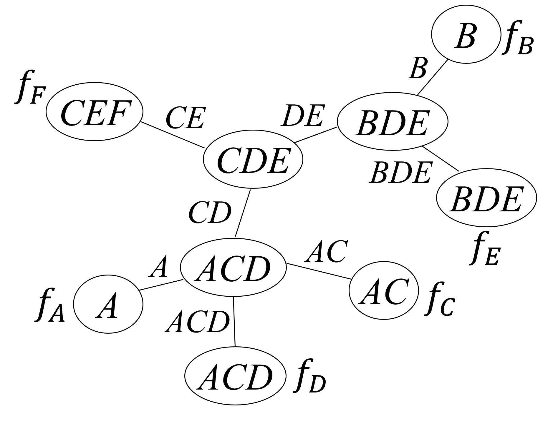
(a) base jointree, width $w=2$

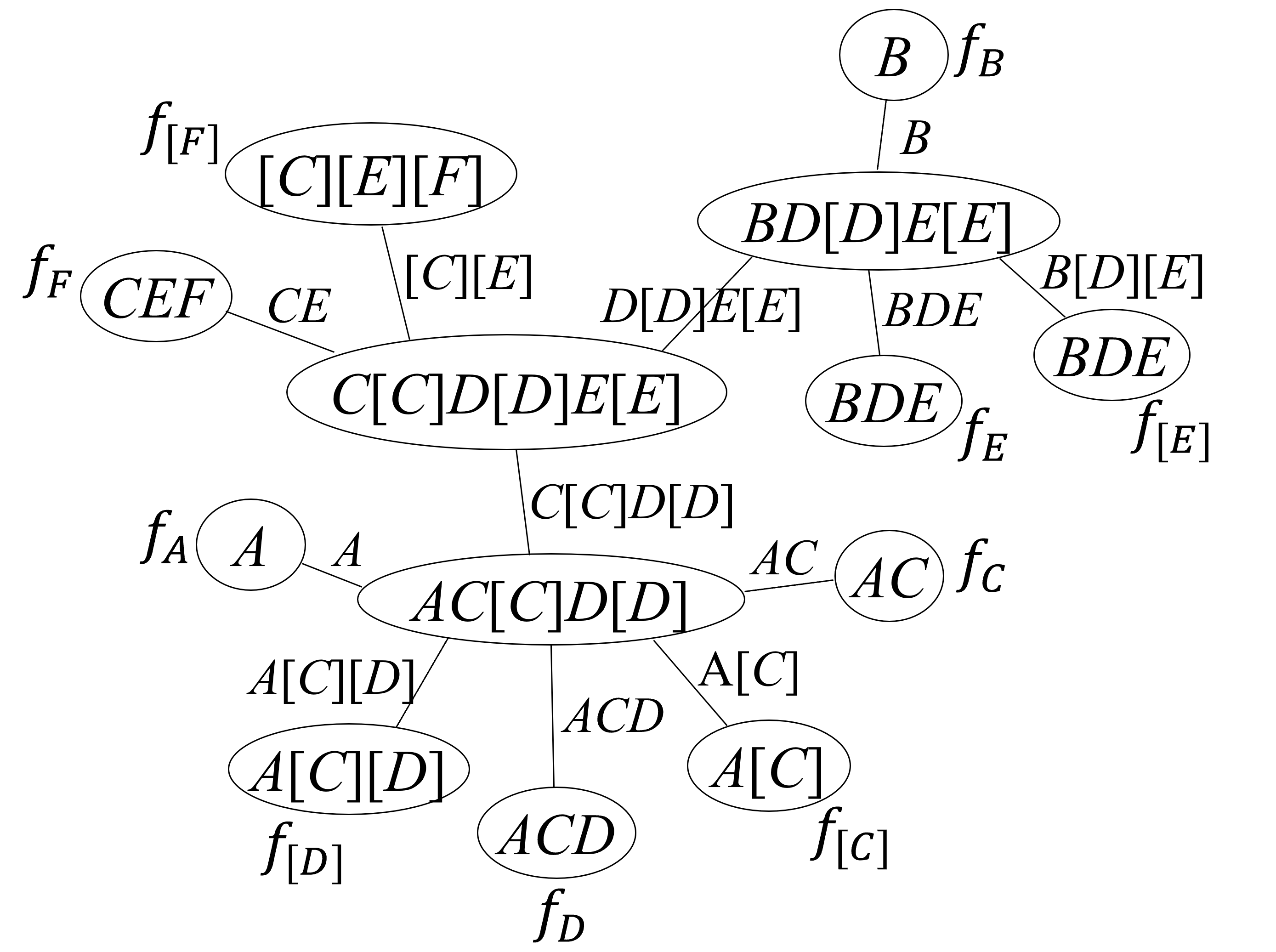
(b) twin jointree, width $w^{t}=5$

Figure 8: A base jointree and its twin jointree, where $w^{t}=2w+1$.

(a) base network, treewidth $w=2$

(b) twin network, treewidth $w^{t}=4$

Figure 9: A base network and its corresponding twin network, where $w^{t}=2w$.

Appendix B Tightness of Bounds

As we claimed in the paper, Corollaries $1$ and $3$ provide tight bounds for the widths of twin elimination orders defined by Definition $2$, and twin jointrees constructed by Algorithm 1, respectively. Moreover, we provide a concrete example where a base network has treewidth $w$ and its twin network has treewidth $2w$, which suggests that our bound on treewidth in Corollary $2$ may also be tight (we found these examples through exhaustive search which we were able to do on small examples only, given the allotted computational resources).

For the tightness of Corollary $1$, consider the base network $G$ shown in Figure 7(a). The elimination order $\pi=(A,B,F,D,C,E)$ has width of $2.$ The twin network $G^{t}$ for $G$ is shown in Figure 7(b). By Definition $2$, the twin elimination order for $G^{t}$ is $\pi^{t}=(A,B,F,[F],D,[D],C,[C],E,[E])$ which has a width of $5.$

For the tightness of Corollary $3$, Figure 8(a) shows a base jointree for the base network $G$. This base jointree was constructed using elimination order $\pi$ and it has a width of $2$. Figure 8(b) shows a twin jointree constructed by Algorithm 1 which has a width of $5.$

For our last example, Figure 9(a) shows a base network with a treewidth of $2.$ Figure 9(b) shows the corresponding twin network which has a treewidth of $4.$ This shows that if our treewidth bound in Corollary $2$ is not tight, then it is off by at most $1$.

Appendix C Additional Figures

Figure 10(b) shows a thinned jointree for the base network in Figure 10(a). Figure 10(c) shows the corresponding thinned, twin jointree constructed by Algorithm 1 and annotated with the thinned separators (and clusters) as given by Theorem 3. The jointree width is preserved in this case.

(a) base network

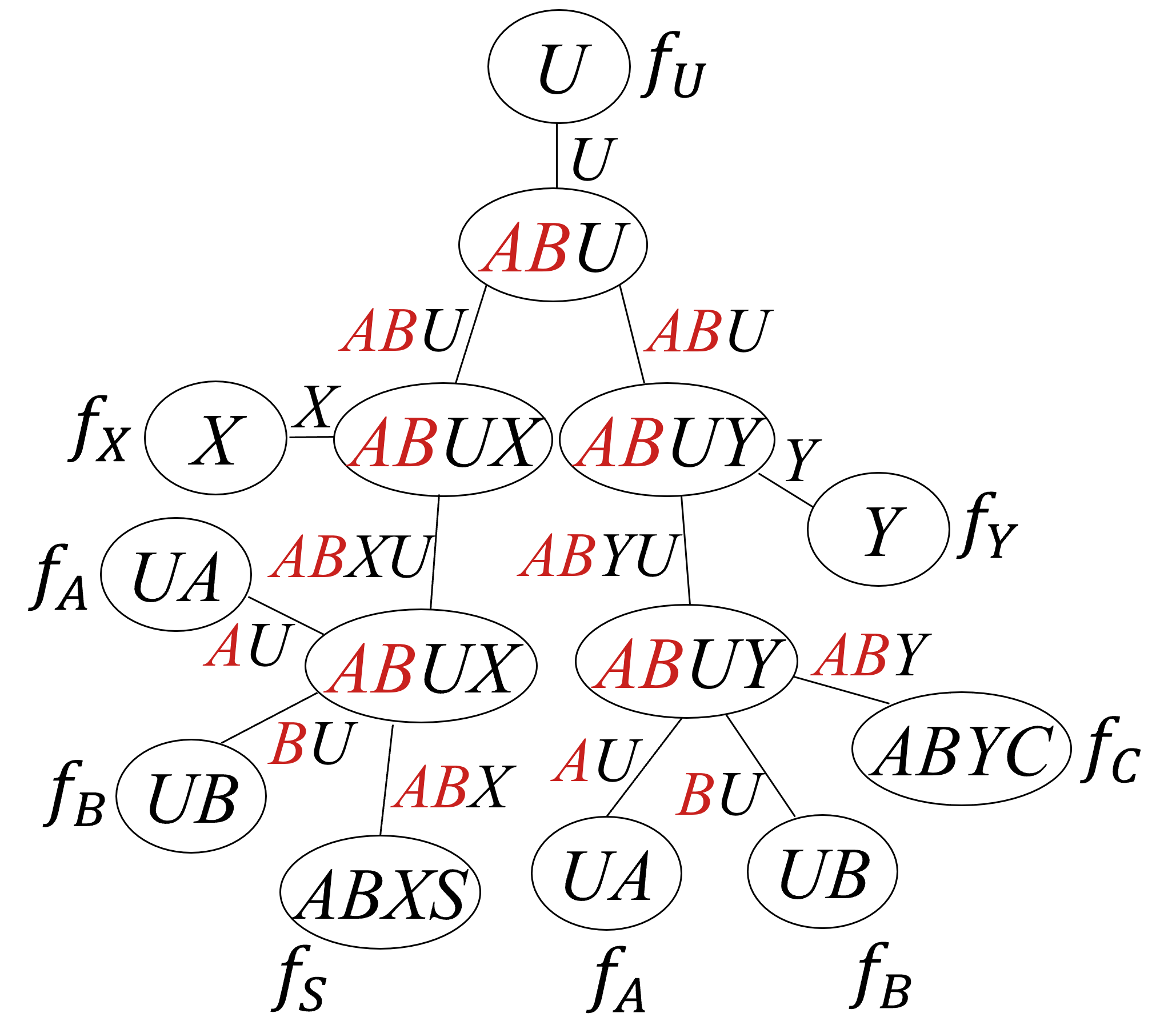
(b) thinned base jointreen (width $3$)

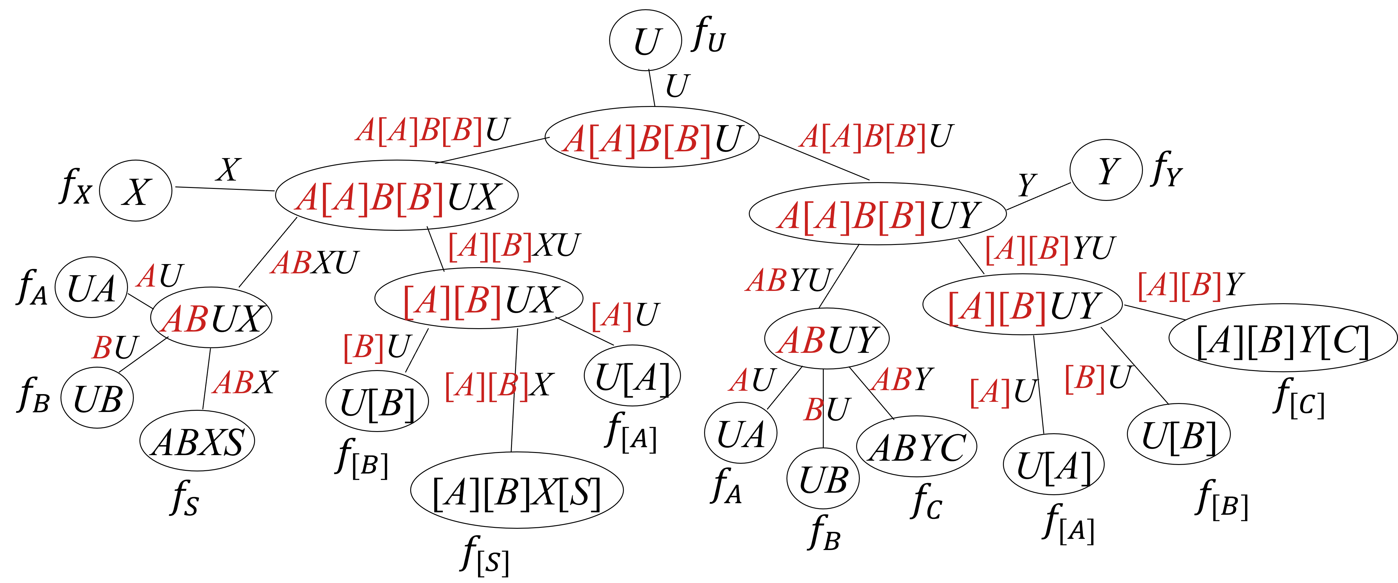
(c) thinned twin jointree (width $3$)

Figure 10: Illustrating the construction of a thinned, twin jointree from a thinned, base jointree.

Appendix D Generalized $N$-World Networks

We show that the bound on treewidth also applies to a more general version of $N$-world networks, called generalized $N$-world networks, that allow any selected, subset of nodes to be duplicated and also allow certain edges between duplicates of the same variable.

Definition 4.

Let $G$ be a base network and let ${\mathbf{X}}$ be any subset of its nodes. A generalized $N$-world network is constructed as follows. We replace each node $X\in{\mathbf{X}}$ with $N$ duplicates denoted as $X^{1},\dots,X^{N}$. For each parent $P$ of $X$, if $P$ is not in ${\mathbf{X}}$, then make $P$ a parent of $X^{1},\dots,X^{N}$; otherwise, make $P^{i}$ a parent of $X^{i}$ for each $i\in 1,\dots,N$. Moreover, for each pair of duplicates $X^{i}$ and $X^{j}$ where $1\leq i<j\leq N$, an edge may be added from $X^{i}$ to $X^{j}$.

Figure 11(b) shows a generalized $3$-world network for the base network in Figure 11(a). The notion of generalized $N$-world networks is significant as it covers a vast subclass of dynamic Bayesian networks, which is widely used for temporal reasoning.

(a) base network

(b) generalized $3$-world network

Figure 11: A base network and a corresponding generalized $3$-world network. Nodes $B,D$ were duplicated and edges $D^{1}\rightarrow D^{2}$, $D^{2}\rightarrow D^{3}$, $D^{1}\rightarrow D^{3}$ were added.

The following result shows that our bound still applies to generalized $N$-world networks. It is worth mentioning that the bound also applies for any subgraphs of a generalized $N$-world network, as the treewidth of any subgraph is no greater than the treewidth of the original network.

Theorem 5.

Let $w$ and $w^{t}$ be the treewidths of a base network and its generalized $N$-world network, then $w^{t}\leq N(w+1)-1$.

Proof.

The proof is similar to the one for Theorem 4. We are assuming here that the duplicated nodes of $G$ are ${\mathbf{Y}}$. We maintain the following invariant: for each $i\in 1\dots,n$ and each node $X^{j}$ ($j\in 1\dots,N$) in $G^{N}_{i}$, $G^{N}_{i}(X^{j})\subseteq\bigcup_{k=1}^{N}G_{i}(X)^{k}$. To show the invariant holds initially, observe that the construction of a generalized $N$-world network involves two steps: duplicating the nodes in ${\mathbf{Y}}$ and adding edges between the duplicates of ${\mathbf{Y}}$. After the first step, the invariant holds since an edge is added between two nodes in $G^{N}$ only if the parent-child relationship exists in the base network. We next show that the invariant still holds after the second step. Each time we add an edge from one duplicate $Y^{j}$ to another duplicate $Y^{l}$ ($1\leq j<l\leq N$), $Y^{j}$ becomes a neighbor of $Y^{l}$ and the parents of $Y^{l}$. Since $Y^{j}$, $Y^{l}$ and the parents of $Y^{l}$ all belong to the set $\bigcup_{k=1}^{N}G_{1}(Y)^{k}$, $G^{N}_{1}(Y^{j})$ and $G^{N}_{1}(Y^{l})$ are still subsets of $\bigcup_{k=1}^{N}G_{1}(Y)^{k}$ after the edge is added. Similarly, for each parent $P^{s}$ of $Y^{l}$ where $1\leq s\leq N$, since $Y^{j}$ already belongs to the set $\bigcup_{k=1}^{N}G_{1}(P)^{k}$, $G^{N}_{1}(P^{s})$ remains a subset of $\bigcup_{k=1}^{N}G_{1}(P)^{k}$ after the edge is added. It follows inductively that the invariant still holds after all edges are added.

We next show that the invariant holds after each elimination step. This can be done with a same inductive argument as Lemma 3. Suppose the invariant holds in $G^{N}_{i-1}$ and we want to eliminate $\{Y^{k}\}_{k=1}^{N}$, we consider how the eliminations affect the neighbors of each node $X^{j}$ in $G^{N}_{i-1}$. Suppose $Y$ is not in $G_{i-1}(X)$, then by the inductive assumption, none of $\{Y^{k}\}_{k=1}^{N}$ are in $G^{N}_{i-1}(X^{j})$. Thus $G_{i}(X)=G_{i-1}(X)$ and $G^{N}_{i}(X^{j})=G^{N}_{i-1}(X^{j})$. Suppose $Y$ is in $G_{i-1}(X)$, then $G_{i}(X)=G_{i-1}(X)\cup G_{i-1}(Y)\setminus\{Y\}$ and $G^{N}_{i}(X^{j})\subseteq(\bigcup_{k=1}^{N}{G_{i-1}(X)}^{k})\cup(\bigcup_{k=1}^{N}{G_{i-1}(Y)}^{k})\setminus\{{Y}^{k}\}_{k=1}^{N}=\bigcup_{k=1}^{N}{G_{i}(X)}^{k}$. The inductive assumption holds for both cases.

We finally show that the cluster formed for each $Y^{j}$ ($1\leq j\leq N$), denoted ${\mathbf{C}}^{N}(Y^{j})$, is a subset of $\bigcup_{k=1}^{N}{{\mathbf{C}}(Y)}^{k}$, where ${\mathbf{C}}(Y)=G_{i-1}(Y)$. This is similar to Lemma 4. For each $Y^{j}$, by the definition of variable elimination, the cluster is bounded as ${\mathbf{C}}^{N}(Y^{j})=\bigcup_{k=1}^{j}G^{N}_{i-1}(Y^{k})\subseteq\bigcup_{k=1}^{N}{G_{i-1}(Y)}^{k}=\bigcup_{k=1}^{N}{\mathbf{C}}(Y)^{k}$. We can then conclude the bound on widths and treewidths. ∎

Appendix E More on Experiments

Our experiments were run on 2.60GHz Intel Xeon E5-2670 CPU with 256 GB of memory.

In the main paper, we plotted the jointree widths for random networks with a maximum number of parents ($p=5$). Here we show the complete experimental results for the random networks with $p=3,5,7$ generated according to the method of Darwiche [2020] which we discussed in the main paper. We record the widths and normalized widths for each twin jointrees. Recall that if a jointree has clusters ${\mathbf{C}}_{1},\ldots,{\mathbf{C}}_{n}$, then the normalized width is $\log_{2}\sum_{i=1}^{n}2^{|{\mathbf{C}}_{i}|}$. Table 1 shows the complete results for rNET and Table 2 shows the complete results for rSCM.

In addition, we report results on random networks generated by a second method proposed in Ide and Cozman [2002]. Given a number of nodes $n$ and a maximum degree $d$ for each node, the method generates a random network by repeatedly adding/removing random edges from the current DAG. We refer to these random networks as rNET2. Similarly to what we did for rNET, we then added a unique root as parent for each internal variable in rNET2. We refer to these modified networks as rSCM2. For each combination of $n\in\{50,100,150,200\}$ and $d\in\{5,10,15\}$, we generated $50$ random base networks and reported the average widths and normalized widths for each twin jointree. Table 3 shows the complete results for rNET2 and Table 4 shows the complete results for rSCM2. The patterns in these tables resemble the ones for rNET and rSCM.

num vars	max pars	stats	BASE- MF		TWIN- ALG1		TWIN- MF		BASE- MF-RLS		TWIN- THM3		TWIN- MF-RLS
			wd	nwd	wd	nwd	wd	nwd	wd	nwd	wd	nwd	wd	nwd
50	3	mean	7.5	11.5	14.4	17.1	10.0	14.0	5.2	11.9	7.6	13.2	5.6	13.0
		std	1.4	0.9	2.8	2.4	2.0	1.4	1.0	0.7	1.2	0.7	1.2	0.7
	5	mean	14.3	17.4	26.8	29.2	15.9	19.6	7.2	15.0	10.0	16.2	7.3	16.0
		std	2.0	1.7	4.0	3.8	1.9	1.7	1.2	0.8	2.1	0.9	1.1	0.8
	7	mean	19.5	22.4	36.9	39.1	20.4	24.1	8.9	17.1	12.2	18.3	8.9	18.1
		std	2.0	1.9	4.1	3.9	1.8	1.7	0.8	0.7	2.4	0.8	0.9	0.7
75	3	mean	10.2	13.8	18.9	21.5	14.5	17.9	6.1	12.9	8.6	14.3	6.9	14.0
		std	1.9	1.5	3.6	3.4	2.4	2.0	1.6	0.8	1.9	0.9	1.9	0.8
	5	mean	21.3	23.9	39.1	41.1	23.9	27.2	8.4	16.4	11.9	17.8	9.1	17.5
		std	2.3	2.2	5.1	4.9	3.0	2.7	1.6	0.8	2.2	1.0	1.8	0.8
	7	mean	28.8	31.4	54.0	56.0	30.3	33.7	11.0	18.6	16.4	21.2	11.7	19.7
		std	2.6	2.5	5.2	5.2	2.2	2.1	1.9	0.9	4.1	2.4	2.0	0.9
100	3	mean	13.7	16.7	25.1	27.5	19.9	22.8	7.1	13.8	10.2	15.3	8.3	14.9
		std	2.4	2.1	4.7	4.4	3.3	2.8	1.7	0.8	2.2	1.2	1.9	0.9
	5	mean	27.1	29.7	50.8	52.9	31.4	34.5	9.5	17.1	13.5	18.9	11.2	18.4
		std	2.5	2.5	5.1	5.0	3.6	3.2	2.2	0.6	2.9	1.5	3.0	0.9
	7	mean	38.7	40.9	72.9	74.7	40.8	43.8	14.5	20.3	22.9	26.6	15.9	21.9
		std	3.5	3.4	6.7	6.5	3.3	3.2	3.3	1.5	7.1	5.8	3.4	1.8
125	3	mean	16.7	19.6	30.8	33.0	26.9	29.3	7.9	14.6	10.5	16.1	9.2	15.9
		std	2.1	1.9	4.0	3.8	3.9	3.6	2.0	0.8	2.3	1.2	2.3	1.0
	5	mean	34.9	37.3	65.1	66.9	39.1	42.1	12.1	18.3	17.2	21.4	14.8	20.3
		std	3.1	2.9	5.9	5.7	3.6	3.2	2.4	1.0	3.8	2.5	3.6	1.9
	7	mean	47.9	50.1	89.8	91.7	50.6	53.5	19.7	23.7	32.5	35.1	21.7	26.1
		std	3.2	3.1	6.8	6.7	3.8	3.6	4.2	3.3	8.7	8.3	4.5	3.7
150	3	mean	20.3	22.9	36.9	38.9	31.8	34.2	8.6	15.2	11.1	16.7	9.8	16.4
		std	2.4	2.3	4.7	4.7	4.2	3.9	2.1	0.8	2.2	1.1	2.5	1.1
	5	mean	41.4	43.6	76.9	78.6	49.1	51.7	14.6	19.7	21.2	24.7	18.6	22.8
		std	3.3	3.1	7.4	7.2	6.3	5.8	2.9	1.8	5.3	4.5	4.0	3.2
	7	mean	56.7	58.7	106.7	108.2	60.6	63.3	22.5	26.1	36.8	39.3	25.6	29.4
		std	4.1	3.8	8.1	7.9	3.6	3.5	4.8	3.9	9.6	9.1	5.1	4.5
200	3	mean	25.8	28.2	47.2	49.1	42.9	44.8	10.7	16.4	13.6	18.3	12.3	17.9
		std	2.5	2.5	4.9	4.9	5.4	5.2	2.9	1.5	2.9	1.5	3.2	1.9
	5	mean	55.1	57.2	102.4	104.0	65.7	68.0	19.9	23.8	29.5	32.3	26.0	29.4
		std	3.6	3.5	7.8	7.6	7.0	6.8	4.2	3.3	8.1	7.6	6.1	5.3
	7	mean	75.3	77.4	141.5	143.1	80.4	82.7	34.3	37.1	57.5	59.8	39.0	42.3
		std	4.1	3.9	8.4	8.2	4.3	4.1	4.8	4.7	10.2	10.2	5.1	4.8
250	3	mean	31.6	34.0	58.1	60.0	55.7	57.4	12.1	17.4	15.0	19.5	14.1	19.2
		std	3.1	2.9	6.1	6.0	6.4	6.2	2.8	1.5	3.1	2.1	3.2	2.0
	5	mean	68.6	70.5	128.5	129.9	84.9	86.8	25.8	28.9	38.9	41.3	36.1	38.9
		std	4.1	3.8	7.9	7.7	9.9	9.6	4.7	4.4	9.4	9.2	7.5	7.1
	7	mean	95.6	97.4	180.3	181.7	102.7	104.7	44.2	46.7	74.6	76.6	49.5	52.7
		std	4.9	4.7	10.1	9.9	5.5	5.3	6.5	6.3	13.2	13.1	6.8	6.7
300	3	mean	40.1	42.3	73.9	75.6	69.9	71.5	13.9	18.4	17.4	21.2	16.3	20.5
		std	3.9	3.6	7.6	7.3	8.0	7.9	2.7	1.8	3.9	3.3	3.4	2.7
	5	mean	82.4	84.1	153.3	154.5	104.8	106.4	32.8	35.7	50.1	52.3	46.1	48.6
		std	4.7	4.5	9.7	9.6	14.6	14.3	5.4	5.3	10.4	10.2	8.8	8.5
	7	mean	114.3	116.0	215.9	217.1	123.4	125.2	55.5	58.0	95.2	97.1	62.2	65.3
		std	4.1	4.0	8.4	8.4	5.8	5.6	7.2	7.2	14.3	14.2	7.5	7.3

Table 1: Widths (wd) and normalized widths (nwd) of various twin jointrees under rNET Darwiche [2020]. Refer to the main paper for the details of different jointree construction methods. All the thinned jointrees are constructed by bounding the functional chain lengths by $10$; see Chen and Darwiche [2022] for details.

num vars	max pars	stats	BASE- MF		TWIN- ALG1		TWIN- MF		BASE- MF-RLS		TWIN- THM3		TWIN- MF-RLS
			wd	nwd	wd	nwd	wd	nwd	wd	nwd	wd	nwd	wd	nwd
50	3	mean	7.5	11.9	14.4	17.4	14.0	17.1	11.1	15.6	14.7	18.3	14.2	18.3
		std	1.4	0.7	2.8	2.2	2.7	2.3	2.5	2.0	3.0	2.3	2.6	2.2
	5	mean	14.3	17.4	26.9	29.3	26.4	28.9	19.0	22.7	23.5	26.5	22.9	26.2
		std	2.0	1.7	4.0	3.8	3.9	3.7	2.5	2.2	3.3	2.9	2.8	2.4
	7	mean	19.5	22.4	37.0	39.3	37.0	39.1	24.3	27.7	31.0	33.5	29.4	32.4
		std	2.0	1.9	4.1	3.9	4.2	4.0	2.6	2.2	3.5	3.2	3.4	2.9
75	3	mean	10.2	14.0	18.9	21.6	18.5	21.3	14.9	18.5	19.1	22.1	18.1	21.5
		std	1.9	1.3	3.6	3.4	3.6	3.4	3.2	2.8	4.1	3.6	3.7	3.2
	5	mean	21.3	23.9	39.1	41.1	38.5	40.7	26.9	29.7	33.5	35.8	31.8	34.5
		std	2.3	2.2	5.1	4.9	5.1	4.9	2.7	2.5	3.8	3.6	3.7	3.3
	7	mean	28.8	31.4	54.1	56.2	53.9	55.9	34.5	36.9	44.9	46.9	42.3	44.5
		std	2.6	2.5	5.3	5.3	5.2	5.1	3.4	3.1	5.5	5.2	4.9	4.6
100	3	mean	13.7	16.8	25.1	27.5	24.4	26.9	19.5	22.4	24.9	27.1	23.1	25.9
		std	2.4	2.0	4.7	4.4	4.7	4.4	3.6	3.2	4.6	4.2	4.0	3.8
	5	mean	27.1	29.7	50.8	52.9	50.8	52.8	34.6	37.0	43.9	45.8	40.5	42.8
		std	2.5	2.5	5.4	5.2	5.1	5.0	3.9	3.7	5.4	5.2	4.8	4.5
	7	mean	38.7	40.9	73.0	74.8	72.8	74.5	45.8	47.8	61.3	62.9	57.4	59.4
		std	3.5	3.4	6.7	6.5	6.8	6.7	4.7	4.5	7.9	7.7	7.4	7.1
125	3	mean	16.7	19.6	30.8	33.0	30.5	32.7	23.8	26.5	29.5	31.8	28.0	30.6
		std	2.1	1.8	4.0	3.8	3.7	3.5	2.8	2.6	4.0	3.6	3.6	3.3
	5	mean	34.9	37.3	65.1	66.9	64.9	66.6	44.4	46.5	56.5	58.1	51.8	54.0
		std	3.1	2.9	5.9	5.7	6.1	6.0	5.0	4.7	7.0	6.7	5.6	5.4
	7	mean	47.9	50.1	90.1	91.9	89.9	91.6	55.4	57.5	76.1	77.6	71.2	73.2
		std	3.2	3.1	6.7	6.6	6.6	6.4	3.9	3.7	7.3	7.0	6.5	6.2
150	3	mean	20.3	22.9	36.9	38.9	36.2	38.2	27.3	30.0	34.0	36.1	31.9	34.3
		std	2.4	2.3	4.7	4.7	4.4	4.3	3.5	3.3	4.4	4.2	4.5	4.2
	5	mean	41.4	43.6	76.9	78.6	76.3	77.9	50.6	52.5	65.3	66.8	60.6	62.5
		std	3.3	3.1	7.4	7.2	6.9	6.9	4.3	4.2	7.3	7.1	6.5	6.2
	7	mean	56.7	58.7	106.7	108.2	106.0	107.5	65.7	67.4	91.1	92.4	83.2	85.0
		std	4.1	3.8	8.1	7.9	7.5	7.4	4.5	4.4	8.0	7.9	7.0	6.9
200	3	mean	25.8	28.3	47.2	49.1	46.2	48.2	35.5	37.6	44.2	45.9	40.7	42.8
		std	2.5	2.5	5.0	4.9	4.9	4.9	4.5	4.3	6.4	6.1	5.6	5.3
	5	mean	55.0	57.2	102.5	104.1	102.0	103.5	67.7	69.4	88.7	90.0	82.6	84.1
		std	3.6	3.5	7.3	7.2	7.6	7.5	5.5	5.4	8.8	8.6	7.8	7.6
	7	mean	75.3	77.4	141.5	143.1	75.3	77.4	87.0	88.6	124.6	125.8	115.2	116.7
		std	4.1	3.9	8.4	8.2	4.1	3.9	4.6	4.4	9.2	9.2	8.4	8.3
250	3	mean	31.6	34.0	58.1	60.0	57.5	59.4	43.8	45.8	54.3	55.9	49.8	51.9
		std	3.1	3.0	6.0	6.0	6.6	6.5	5.2	4.9	7.7	7.4	6.3	6.0
	5	mean	68.6	70.5	128.5	129.9	127.1	128.5	82.1	83.6	110.3	111.5	101.7	103.2
		std	4.1	3.8	7.9	7.7	7.2	7.1	5.6	5.5	8.9	8.8	7.2	7.1
	7	mean	95.7	97.4	180.4	181.7	179.3	180.7	109.1	110.4	157.5	158.7	146.6	147.9
		std	4.9	4.7	10.1	9.9	8.9	8.8	6.0	5.9	12.2	12.2	10.9	10.8
300	3	mean	40.1	42.3	73.9	75.6	72.4	74.1	54.1	55.8	66.7	68.1	61.8	63.6
		std	3.9	3.6	7.6	7.3	7.5	7.4	5.1	5.1	6.8	6.7	7.1	7.0
	5	mean	82.5	84.1	153.3	154.5	152.7	154.0	99.1	100.4	135.0	136.2	124.3	125.8
		std	4.7	4.5	9.7	9.6	10.4	10.3	6.3	6.2	10.3	10.2	9.9	9.8
	7	mean	114.4	116.0	215.9	217.2	215.1	216.3	131.5	132.7	194.1	195.2	178.8	180.1
		std	4.1	4.0	8.4	8.3	9.1	9.1	5.7	5.6	12.8	12.7	11.2	11.1

Table 2: Widths (wd) and normalized widths (nwd) of various twin jointrees under rSCM Darwiche [2020]. Refer to the main paper for the details of different jointree construction methods. All the thinned jointrees are constructed by bounding the functional chain lengths by $10$; see Chen and Darwiche [2022] for details.

num vars	max degree	stats	BASE- MF		TWIN- ALG1		TWIN- MF		BASE- MF-RLS		TWIN- THM3		TWIN- MF-RLS
			wd	nwd	wd	nwd	wd	nwd	wd	nwd	wd	nwd	wd	nwd
50	5	mean	20.0	22.4	37.3	39.0	20.3	23.6	8.7	14.5	13.5	17.1	8.7	15.5
		std	1.3	1.1	3.3	3.1	1.3	1.1	1.4	0.6	2.9	1.8	1.4	0.7
	10	mean	32.9	35.4	55.5	57.7	32.9	36.4	13.7	18.6	21.6	24.7	13.7	19.6
		std	1.0	0.9	11.9	11.3	1.0	0.9	1.8	1.0	6.0	4.5	1.8	1.0
	15	mean	38.1	40.7	62.5	64.9	38.1	41.7	19.7	23.4	30.6	33.1	19.7	24.4
		std	1.1	0.9	15.6	14.8	1.1	0.9	2.1	1.6	8.3	7.2	2.1	1.6
100	5	mean	40.0	41.8	76.7	78.1	40.1	42.7	14.5	18.4	23.5	25.8	14.6	19.4
		std	1.2	1.4	6.1	5.9	1.7	1.5	2.1	1.6	5.0	4.6	2.1	1.6
	10	mean	65.1	67.4	110.6	112.7	65.5	68.6	33.0	35.9	52.3	54.5	33.0	36.9
		std	1.7	1.5	25.1	24.3	1.8	1.5	2.5	2.4	11.8	11.2	2.5	2.4
	15	mean	75.1	77.5	114.7	117.1	75.2	78.5	45.3	48.0	66.0	68.5	45.3	49.0
		std	1.8	1.6	33.0	32.2	1.8	1.6	3.1	3.1	18.7	17.7	3.1	3.1
150	5	mean	59.7	61.2	110.6	112.0	60.3	62.4	21.5	24.5	36.6	38.6	21.5	25.5
		std	2.6	2.3	17.2	16.8	2.5	2.3	2.5	2.3	7.8	7.4	2.5	2.3
	10	mean	97.1	99.0	159.6	161.7	97.3	100.1	49.8	52.5	80.9	83.1	49.8	53.5
		std	2.0	1.8	37.0	36.7	2.0	1.8	3.6	3.6	20.1	19.3	3.6	3.6
	15	mean	109.7	111.8	168.9	171.3	109.8	112.8	66.7	69.1	92.7	95.3	72.3	75.6
		std	2.5	2.2	49.8	49.2	2.5	2.3	4.2	4.2	28.4	27.6	4.2	4.2
200	3	mean	109.7	111.8	168.9	171.3	109.8	112.8	66.7	69.1	92.7	95.3	72.3	75.6
		std	3.0	2.8	23.3	22.9	2.6	2.5	3.3	3.3	10.0	9.6	3.2	3.2
	5	mean	127.0	128.5	193.6	195.8	127.2	129.6	65.0	67.4	97.2	99.6	65.0	68.4
		std	2.8	2.7	56.4	55.9	3.0	2.9	4.7	4.6	27.8	27.0	4.7	4.6
	7	mean	141.1	142.7	210.8	212.9	141.3	143.9	82.9	85.2	121.3	123.7	82.9	86.3
		std	3.2	3.1	61.0	60.6	3.3	3.1	4.8	4.7	33.9	33.2	4.8	4.7

Table 3: Widths (wd) and normalized widths (nwd) of various twin jointrees under rNET2 Ide and Cozman [2002]. Refer to the main paper for the details of different jointree construction methods. All the thinned jointrees are constructed by bounding the functional chain lengths by $10$; see Chen and Darwiche [2022] for details.

num vars	max degree	stats	BASE- MF		TWIN- ALG1		TWIN- MF		BASE- MF-RLS		TWIN- THM3		TWIN- MF-RLS
			wd	nwd	wd	nwd	wd	nwd	wd	nwd	wd	nwd	wd	nwd
50	5	mean	20.0	22.4	36.2	39.9	37.2	39.2	27.9	30.2	39.6	41.3	37.1	39.1
		std	1.3	1.1	2.4	2.3	2.7	2.4	2.0	2.0	3.4	3.1	2.9	2.6
	10	mean	32.9	35.4	64.8	66.7	64.9	66.8	37.4	39.8	54.0	55.8	50.6	52.9
		std	1.0	0.9	2.4	2.3	2.5	2.5	1.5	1.2	3.1	2.9	2.3	2.3
	15	mean	38.1	40.7	75.3	77.4	76.4	78.5	40.8	43.4	61.1	63.2	60.3	62.5
		std	1.1	0.9	2.4	2.3	3.4	3.1	1.3	1.2	3.5	3.4	3.4	3.4
100	5	mean	40.1	41.7	78.4	79.8	77.7	79.1	54.8	56.2	80.6	81.8	74.3	75.7
		std	1.5	1.4	3.6	3.5	3.5	3.3	3.1	3.1	6.2	6.1	4.7	4.6
	10	mean	65.1	67.4	129.3	131.0	128.6	130.4	75.1	76.6	116.2	117.5	106.4	108.2
		std	1.7	1.5	3.6	3.4	3.9	3.6	2.5	2.3	5.6	5.4	4.1	4.0
	15	mean	75.1	77.5	149.6	151.5	149.3	151.2	81.2	83.1	131.0	132.5	125.7	127.8
		std	1.8	1.6	3.8	3.5	3.4	3.3	2.2	2.0	5.0	4.9	4.9	4.8
150	5	mean	59.7	61.1	118.5	119.7	118.1	119.4	83.0	84.3	125.1	126.2	113.8	115.0
		std	2.5	2.3	4.8	4.7	4.9	4.8	3.7	3.6	6.1	6.0	4.5	4.4
	10	mean	97.1	99.0	193.4	194.9	193.3	194.8	111.1	112.5	174.7	175.8	161.1	162.7
		std	2.0	1.8	4.2	4.0	4.2	4.0	2.3	2.2	5.5	5.5	5.0	4.9
	15	mean	109.7	91.8	218.8	220.4	218.8	220.4	120.3	121.9	196.6	197.9	186.0	187.7
		std	2.5	2.2	5.2	5.0	5.4	5.1	2.9	2.7	6.0	5.9	5.4	5.3
200	5	mean	75.6	76.6	150.7	151.8	150.8	151.9	102.5	103.6	155.0	156.1	143.3	144.4
		std	2.8	2.6	5.6	5.5	5.3	5.2	4.9	4.8	7.2	7.1	5.4	5.4
	10	mean	127.0	128.5	253.4	254.6	252.7	254.0	149.4	148.6	233.0	234.2	212.9	214.3
		std	2.8	2.7	5.5	5.5	4.5	4.4	3.4	3.4	7.7	7.7	6.2	6.1
	15	mean	141.1	142.7	281.7	283.0	281.5	282.8	156.3	159.6	255.6	256.7	238.6	240.2
		std	3.2	3.1	6.4	6.2	6.5	6.4	4.3	4.2	9.7	9.7	7.0	7.0

Table 4: Widths (wd) and normalized widths (nwd) of various twin jointrees under rSCM2 Ide and Cozman [2002]. Refer to the main paper for the details of different jointree construction methods. All the thinned jointrees are constructed by bounding the functional chain lengths by $10$; see Chen and Darwiche [2022] for details.

References

- Avin et al. [2005] Chen Avin, Ilya Shpitser, and Judea Pearl. Identifiability of path-specific effects. In IJCAI, pages 357–363. Professional Book Center, 2005.
- Balke and Pearl [1994a] Alexander Balke and Judea Pearl. Counterfactual probabilities: Computational methods, bounds and applications. In UAI, pages 46–54. Morgan Kaufmann, 1994.
- Balke and Pearl [1994b] Alexander Balke and Judea Pearl. Probabilistic evaluation of counterfactual queries. In AAAI, pages 230–237. AAAI Press / The MIT Press, 1994.
- Balke and Pearl [1995] Alexander Balke and Judea Pearl. Counterfactuals and policy analysis in structural models. In UAI, pages 11–18. Morgan Kaufmann, 1995.
- Bareinboim et al. [2021] E. Bareinboim, Juan David Correa, D. Ibeling, and Thomas F. Icard. On Pearl’s hierarchy and the foundations of causal inference. 2021. Technical Report, R-60, Colombia University.
- Chen and Darwiche [2022] Yizuo Chen and Adnan Darwiche. On the definition and computation of causal treewidth. In UAI, volume 180 of Proceedings of Machine Learning Research, pages 368–377. PMLR, 2022.
- Correa et al. [2021] Juan D. Correa, Sanghack Lee, and Elias Bareinboim. Nested counterfactual identification from arbitrary surrogate experiments. In NeurIPS, pages 6856–6867, 2021.
- Cozman [2000] Fábio Gagliardi Cozman. Credal networks. Artif. Intell., 120(2):199–233, 2000.
- Darwiche [2003] Adnan Darwiche. A differential approach to inference in Bayesian networks. J. ACM, 50(3):280–305, 2003.
- Darwiche [2009] Adnan Darwiche. Modeling and Reasoning with Bayesian Networks. Cambridge University Press, 2009.
- Darwiche [2020] Adnan Darwiche. An advance on variable elimination with applications to tensor-based computation. In ECAI, volume 325 of Frontiers in Artificial Intelligence and Applications, pages 2559–2568. IOS Press, 2020.
- Darwiche [2021] Adnan Darwiche. Causal inference with tractable circuits. In WHY Workshop, NeurIPS, 2021. https://arxiv.org/abs/2202.02891.
- Darwiche [2022] Adnan Darwiche. Tractable Boolean and arithmetic circuits. In Pascal Hitzler and Md Kamruzzaman Sarker, editors, Neuro-symbolic Artificial Intelligence: The State of the Art, volume 342, chapter 6. Frontiers in Artificial Intelligence and Applications. IOS Press, 2022.
- Dawid et al. [2017] Philip Dawid, Monica Musio, and Rossella Murtas. The probability of causation. Law, Probability and Risk, (16):163–179, 2017.
- Dean and Kanazawa [1989] Thomas Dean and Keiji Kanazawa. A model for reasoning about persistence and causation. Computational Intelligence, 5, 1989.
- Dechter [1996] Rina Dechter. Bucket elimination: A unifying framework for probabilistic inference. In Proceedings of the Twelfth Annual Conference on Uncertainty in Artificial Intelligence (UAI), pages 211–219, 1996.
- Duarte et al. [2021] Guilherme Duarte, Noam Finkelstein, Dean Knox, Jonathan Mummolo, and Ilya Shpitser. An automated approach to causal inference in discrete settings. CoRR, abs/2109.13471, 2021.
- Evans [2018] Robin J. Evans. Margins of discrete Bayesian networks. The Annals of Statistics, 46(6A):2623 – 2656, 2018.
- Galles and Pearl [1998] David Galles and Judea Pearl. An axiomatic characterization of causal counterfactuals. Foundations of Science, 3(1):151–182, 1998.
- Halpern [2000] Joseph Y Halpern. Axiomatizing causal reasoning. Journal of Artificial Intelligence Research, 12:317–337, 2000.
- Hamscher et al. [1992] Walter Hamscher, Luca Console, and Johan de Kleer, editors. Readings in Model-Based Diagnosis. Morgan Kaufmann Publishers Inc., San Francisco, CA, USA, 1992.
- Huang and Darwiche [2023] Haiying Huang and Adnan Darwiche. An algorithm and complexity results for causal unit selection. In 2nd Conference on Causal Learning and Reasoning, Proceedings of Machine Learning Research, 2023.
- Ide and Cozman [2002] Jaime Shinsuke Ide and Fábio Gagliardi Cozman. Random generation of bayesian networks. In SBIA, volume 2507 of Lecture Notes in Computer Science, pages 366–375. Springer, 2002.
- Jung et al. [2020] Yonghan Jung, Jin Tian, and Elias Bareinboim. Learning causal effects via weighted empirical risk minimization. In NeurIPS, 2020.
- Jung et al. [2021a] Yonghan Jung, Jin Tian, and Elias Bareinboim. Estimating identifiable causal effects on markov equivalence class through double machine learning. In ICML, volume 139 of Proceedings of Machine Learning Research, pages 5168–5179. PMLR, 2021.
- Jung et al. [2021b] Yonghan Jung, Jin Tian, and Elias Bareinboim. Estimating identifiable causal effects through double machine learning. In AAAI, pages 12113–12122. AAAI Press, 2021.
- Kjaerulff [1990] Uffe Kjaerulff. Triangulation of graphs – algorithms giving small total state space. 1990. Technical Report R-90-09, Department of Mathematics and Computer Science, University of Aalborg, Denmark.
- Kjærulff [1994] Uffe Kjærulff. Reduction of computational complexity in bayesian networks through removal of weak dependences. In UAI, pages 374–382. Morgan Kaufmann, 1994.
- Koller and Friedman [2009] Daphne Koller and Nir Friedman. Probabilistic Graphical Models - Principles and Techniques. MIT Press, 2009.
- Larrañaga et al. [1997] Pedro Larrañaga, Cindy M. H. Kuijpers, Mikel Poza, and Roberto H. Murga. Decomposing bayesian networks: triangulation of the moral graph with genetic algorithms. Statistics and Computing, 7, 1997.
- Lauritzen and Spiegelhalter [1988] S. L. Lauritzen and D. J. Spiegelhalter. Local computations with probabilities on graphical structures and their application to expert systems. Journal of the Royal Statistical Society. Series B (Methodological), 50(2):157–224, 1988.
- Li and Pearl [2022] Ang Li and Judea Pearl. Unit selection with nonbinary treatment and effect. CoRR, abs/2208.09569, 2022.
- Mauá and Cozman [2020] Denis Deratani Mauá and Fabio Gagliardi Cozman. Thirty years of credal networks: Specification, algorithms and complexity. International Journal of Approximate Reasoning, 126:133–157, 2020.
- Mengshoel et al. [2010] Ole J. Mengshoel, Mark Chavira, Keith Cascio, Scott Poll, Adnan Darwiche, and N. Serdar Uckun. Probabilistic model-based diagnosis: An electrical power system case study. IEEE Trans. Syst. Man Cybern. Part A, 40(5):874–885, 2010.
- Mueller et al. [2022] Scott Mueller, Ang Li, and Judea Pearl. Causes of effects: Learning individual responses from population data. In IJCAI, pages 2712–2718. ijcai.org, 2022.
- Pearl and Mackenzie [2018] Judea Pearl and Dana Mackenzie. The Book of Why: The New Science of Cause and Effect. Basic Books, 2018.
- Pearl [1988] Judea Pearl. Probabilistic Reasoning in Intelligent Systems: Networks of Plausible Inference. Morgan Kaufmann, 1988.
- Pearl [1995] Judea Pearl. Causal diagrams for empirical research. Biometrika, 82(4):669–688, 1995.
- Pearl [1999] Judea Pearl. Probabilities of causation: Three counterfactual interpretations and their identification. Synth., 121(1-2):93–149, 1999.
- Pearl [2009] Judea Pearl. Causality. Cambridge University Press, second edition, 2009.
- Peters et al. [2017] Jonas Peters, Dominik Janzing, and Bernhard Schölkopf. Elements of Causal Inference: Foundations and Learning Algorithms. MIT Press, 2017.
- Robertson and Seymour [1986] Neil Robertson and Paul D. Seymour. Graph minors. II. algorithmic aspects of tree-width. J. Algorithms, 7(3):309–322, 1986.
- Rosset et al. [2018] Denis Rosset, Nicolas Gisin, and Elie Wolfe. Universal bound on the cardinality of local hidden variables in networks. Quantum Info. Comput., 18(11–12):910–926, sep 2018.
- Shpitser and Pearl [2006] Ilya Shpitser and Judea Pearl. Identification of joint interventional distributions in recursive semi-markovian causal models. In AAAI, pages 1219–1226. AAAI Press, 2006.
- Shpitser and Pearl [2007] Ilya Shpitser and Judea Pearl. What counterfactuals can be tested. In UAI, pages 352–359. AUAI Press, 2007.
- Shpitser and Pearl [2008] Ilya Shpitser and Judea Pearl. Complete identification methods for the causal hierarchy. J. Mach. Learn. Res., 9:1941–1979, 2008.
- Spirtes et al. [2000] Peter Spirtes, Clark Glymour, and Richard Scheines. Causation, Prediction, and Search, Second Edition. Adaptive computation and machine learning. MIT Press, 2000.
- Tian and Pearl [2000] Jin Tian and Judea Pearl. Probabilities of causation: Bounds and identification. Ann. Math. Artif. Intell., 28(1-4):287–313, 2000.
- Tian and Pearl [2002] Jin Tian and Judea Pearl. A general identification condition for causal effects. In AAAI/IAAI, pages 567–573. AAAI Press / The MIT Press, 2002.
- Zaffalon et al. [2020] Marco Zaffalon, Alessandro Antonucci, and Rafael Cabañas. Structural causal models are (solvable by) credal networks. In International Conference on Probabilistic Graphical Models, PGM, volume 138 of Proceedings of Machine Learning Research, pages 581–592. PMLR, 2020.
- Zaffalon et al. [2021] Marco Zaffalon, Alessandro Antonucci, and Rafael Cabañas. Causal Expectation-Maximisation. In WHY Workshop, NeurIPS, 2021. https://arxiv.org/abs/2011.02912.
- Zaffalon et al. [2022] Marco Zaffalon, Alessandro Antonucci, Rafael Cabañas, David Huber, and Dario Azzimonti. Bounding counterfactuals under selection bias. In PGM, volume 186 of Proceedings of Machine Learning Research, pages 289–300. PMLR, 2022.
- Zhang and Poole [1994] Nevin Lianwen Zhang and David L. Poole. Intercausal independence and heterogeneous factorization. In UAI, pages 606–614. Morgan Kaufmann, 1994.
- Zhang et al. [2021] Junzhe Zhang, Jin Tian, and Elias Bareinboim. Partial counterfactual identification from observational and experimental data. CoRR, abs/2110.05690, 2021.
- Zhang et al. [2022] Junzhe Zhang, Jin Tian, and Elias Bareinboim. Partial counterfactual identification from observational and experimental data. In ICML, volume 162 of Proceedings of Machine Learning Research, pages 26548–26558. PMLR, 2022.