A Unified Framework for Analyzing and Optimizing a Class of Convex Inequity Measures

Abstract

We propose a new unified framework for analyzing a new parameterized class of convex inequity measures suitable for optimization contexts. First, we propose a new class of order-based inequity measures, discuss their properties, and derive axiomatic characterizations for such measures. Then, we introduce our proposed class of convex inequity measures, discuss their theoretical properties in an absolute and relative sense, and derive an equivalent dual representation of these measures as a robustified order-based inequity measure over their dual sets. Importantly, this dual representation renders a unified mathematical expression and an alternative geometric characterization for convex inequity measures through their dual sets. Using this representation, we propose a unified framework for optimization problems with a convex inequity measure objective or constraint, including reformulations and solution methods. Finally, we provide stability results that quantify the impact of employing different convex inequity measures on the optimal value and solution of the resulting optimization problem. Our numerical results demonstrate the computational efficiency of our proposed framework over existing approaches.

1 Introduction

Equity concerns arise naturally in various decision-making contexts and application domains. Examples of real-life settings where equity is a concern include healthcare management, transportation, facility location, humanitarian operations, and resource allocation (Bertsimas et al., 2013; Breugem et al., 2022; Filippi et al., 2021; Gutjahr and Fischer, 2018; Li et al., 2022; Rahmattalabi et al., 2022; Sun et al., 2022, 2023). Thus, it is necessary to incorporate inequity measures in optimization models to address these concerns and make equitable decisions.

Like other factors in an optimization context, one can account for equity by putting related measures in the objective function or constraints. To illustrate, let us consider the following general setting. Suppose we have $N$ subjects of interest, individuals, or groups that are grouped based on some criteria (e.g., location, income, or race). Let $u_{i}$ represent the impact (or outcome) of a given decision $\bm{x}\in\mathbb{R}^{n}$ on subject $i\in[N]$. For example, in a facility location problem, $\bm{x}$ may represent facility location decisions, and $\bm{u}$ may represent customers’ unmet demand or travel time to the nearest open facility. Using this notation, we define the following general optimization problem.

$$\min_{\bm{x},\,\bm{u}}\Big{\{}f(\bm{u})\,\Big{|}\,\bm{u}=U(\bm{x}),\,\bm{x}\in\mathcal{X}\Big{\}},$$ (1)

where $\mathcal{X}\subseteq\mathbb{R}^{n}$ is the set of constraint on $\bm{x}$ and $U:\mathbb{R}^{n}\rightarrow\mathbb{R}^{N}$ is a function for computing the impact of a given decision on the considered subjects. Formulation (1) seeks to find optimal decisions $\bm{x}\in\mathcal{X}$ that optimize some classical equity-neutral objective function $f(\cdot)$ (often called efficiency or inefficiency measure). For example, in the facility location problem, $f(\cdot)$ may represent the sum of the unmet demand and the total travel time to open facilities. Formulation (1) is equity-neutral because it has no measure to ensure that optimal decisions $\bm{x}$ are equitable. Thus, to ensure equity, the literature typically includes inequity measures in the objective or constraints of the optimization model. For example, let $\phi:\mathbb{R}^{N}\rightarrow\mathbb{R}$ represent an inequity measure. Then, one could incorporate $\phi$ in the objective function of (1) as follows:

$$\min_{\bm{x},\,\bm{u}}\Big{\{}f(\bm{u})+\gamma\phi(\bm{u})\,\Big{|}\,\bm{u}=U(\bm{x}),\,\bm{x}\in\mathcal{X}\Big{\}},$$ (2)

for some $\gamma>0$, which controls the trade-off between efficiency and inequity. Alternatively, one could incorporate $\phi$ in the constraint by imposing an upper bound $\eta>0$ on $\phi$ as follows:

$$\min_{\bm{x},\,\bm{u}}\Big{\{}f(\bm{u})\,\Big{|}\,\phi(\bm{u})\leq\eta,\,\bm{u}=U(\bm{x}),\,\bm{x}\in\mathcal{X}\Big{\}}.$$ (3)

Unfortunately, quantifying equity is challenging because there is no best definition or measure of inequity that is universally accepted. Instead, there is a wide variety of notions and measures to gauge the level of equity in the economics, decision theory, and operations research literature (Karsu and Morton, 2015; Shehadeh and Snyder, 2021). Indeed, different inequity measures may produce remarkably different conclusions (i.e., could yield different solutions with varying impacts on equity). In addition, different measures have different mathematical expressions and characteristics. Hence, the choice of inequity measure has important consequences for the tractability of the resulting equity-promoting optimization models such as (2) and (3). As such, customized optimization frameworks have been proposed to analyze and incorporate inequity measures in different contexts. To see this, in Table 1, we present a set of eight widely employed deviation-based or envy-based inequity measures in the literature.

Table 1: Existing deviation-based inequity measures

Index	Measure	Name
i.	$\max_{i\in[N]}u_{i}-\min_{i\in[N]}u_{i}$	Range
ii.	$\sum_{i=1}^{N}\sum_{j=1}^{N}|u_{i}-u_{j}|$	Gini deviation
iii.	$\max_{i\in[N]}\max_{j\in[N]}|u_{i}-u_{j}|$	Maximum pairwise deviation
iv.	$\sum_{i=1}^{N}|u_{i}-\overline{u}|$	Absolute deviation from mean
v.	$\big{[}\sum_{i=1}^{N}(u_{i}-\overline{u})^{2}\big{]}^{1/2}$	Standard deviation
vi.	$\max_{i\in[N]}|u_{i}-\overline{u}|$	Maximum absolute deviation from mean
vii.	$\max_{i\in[N]}\sum_{j=1}^{N}|u_{i}-u_{j}|$	Maximum sum of pairwise deviation
viii.	$\sum_{i=1}^{N}\max_{j\in[N]}|u_{i}-u_{j}|$	Sum of maximum pairwise deviation

We make the following observations about the measures in Table 1. First, in A, we prove that when $N>3$, only measures (i) and (iii) are equivalent, i.e., $\phi^{\text{(i)}}(\bm{u})=\phi^{\text{(iii)}}(\bm{u})$, and measures (vi) and (vii) are equivalent, i.e., $\phi^{\text{(vii)}}(\bm{u})=N\phi^{\text{(vi)}}(\bm{u})$. Thus, using either (i) or (iii) in models (2) and (3) as an inequity measure will yield optimal solutions with the same impact on equity. Similarly, replacing $\phi^{\text{(vi)}}$ by $\phi^{\text{(vii)}}=N\phi^{\text{(vi)}}$ in (2) (resp. in (3)) scales $\gamma$ (resp. $\eta$) by a factor $N$. Furthermore, since the remaining pairs of measures are not equivalent, incorporating any of them in (2) and (3) may produce different solutions than other measures with varying impacts on equity. Second, these measures have different mathematical expressions. Hence, different reformulations and solution techniques may be required to solve the resulting equity-promoting model that incorporates each. For example, to incorporate measure (i), we can introduce auxiliary variables to linearize the maximum and minimum operators. In contrast, we can introduce conic constraints to reformulate measure (v) or solve the resulting optimization model via non-linear optimization techniques. Unfortunately, to date, we still do not have a unified framework for incorporating inequity measures in optimization problems and analyzing the effect of different inequity measures on optimal solutions and equity.

The above observation and challenges inspire this paper’s main contribution: proposing a new unified framework for analyzing and optimizing a class of convex inequity measures suitable for optimization contexts. This class includes those in Table 1 and other popular measures that satisfy some desirable properties to be specified later. Our proposal is as follows. First, to provide a context within the literature, we discuss popular and desirable mathematical properties commonly used to study inequity measures that we also adopt to characterize our proposed class of convex inequity measures (Section 3). Then, we propose a new class of order-based inequity measures, discuss their properties, and derive axiomatic characterizations for such measures (Section 4). This class of order-based inequity measures is the building block of our proposed unified framework for analyzing convex inequity measures. Specifically, in Section 5, we introduce our proposed class of convex inequity measures, discuss their properties in an absolute and relative sense, and derive an equivalent dual representation of these measures as a robustified order-based inequity measure over their dual sets. Importantly, this dual representation renders a unified mathematical expression and an alternative geometric characterization for convex inequity measures through their dual sets. Consequently, it provides a mechanism for investigating the equivalence of convex inequity measures from a geometric perspective. In addition, we use the dual representation to derive equivalent reformulations of optimization models with a convex inequity measure objective and constraints and develop decomposition methods to solve the reformulations (Section 6). Our numerical results demonstrate the computational efficiency of our proposed reformulations and solution methods over existing ones.

Finally, we conduct stability analyses on the choice of convex inequity measures in optimization models via their dual representations (see Section 7). Specifically, we provide mechanisms to quantify the differences in optimal value and solutions of equity-promoting optimization problems under two different convex inequity measures. We close this section by recognizing that focusing on equity alone may degrade efficiency. However, our paper does not address the trade-off between efficiency and equity. Instead, we provide a unified framework for analyzing and incorporating convex inequity measures in optimization models, which could include inefficiency measures. We discuss the trade-off between considering different equity measures in such models in Section 7.

Notation. For two integers $a$ and $b$ with $a<b$, we define the sets $[a]:=\{1,\dots,a\}$ and $[a,b]_{\mathbb{Z}}:=\{a,a+1,\dots,b\}$. We use boldface letters to denote vectors. In particular, $\bm{e}_{j}$ is the $j$th standard unit vector; $\bm{0}$ and $\bm{1}$ are vectors of zeros and ones respectively, where the dimension will be clear in the context. For a given vector $\bm{x}$, we denote $x_{(i)}$ as the $i$th smallest entry of $\bm{x}$. For two vectors $\bm{x}\in\mathbb{R}^{N}$ and $\bm{y}\in\mathbb{R}^{N}$, we say $\bm{x}$ is majorized by $\bm{y}$, denoted as $\bm{x}\preceq\bm{y}$, if $\sum_{i=1}^{N}x_{i}=\sum_{i=1}^{N}y_{i}$ and $\sum_{i=k}^{N}x_{(i)}\leq\sum_{i=k}^{N}y_{(i)}$ for $k\in[2,N]_{\mathbb{Z}}$. We use $\mathbb{R}_{\uparrow}^{N}$ to denote the set of $\mathbb{R}^{N}$ vectors with entries in ascending order, i.e., $\mathbb{R}_{\uparrow}^{N}=\{\bm{x}\in\mathbb{R}^{N}\mid x_{1}\leq\dots\leq x_{N}\}$. Finally, we use $\operatorname{conv}(C)$ to denote the convex hull of a set $C$.

2 Relevant Literature

The importance of equity has been recognized and well-studied in various settings and research communities for decades. Early efforts and a large body of research later focused on defining appropriate measures to capture inequity and axiomatically characterize these measures (Chakravarty, 2007; Cowell and Kuga, 1981; Donaldson and Weymark, 1980; Foster, 1983; Kakwani, 1980; Kolm, 1976; Thon, 1982). This has led to various notions and measures of inequity, each satisfying a set of axiomatic properties that other measures may or may not satisfy. We refer to Andreoli and Zoli (2020), Chakravarty (1999), Cowell (2000), and Jancewicz (2016) for comprehensive surveys and discussions on popular inequity measures and their axiomatic properties (we discuss relevant properties to our work in Section 3). We limit the scope of this review to studies relevant to our paper that focus on measuring inequity in optimization contexts.

In many practical applications of optimization, especially those arising in the public sector, it is essential to consider the effect (positive or negative) of a given decision among individuals or groups (Jagtenberg and Mason, 2020; Shen et al., 2019; Uhde et al., 2020). In particular, such an effect should be as equitable as possible. Hence, the goal of employing inequity measures in the objective and/or constraints of optimization problems could be quantifying equity of opportunity, outcome, treatment, and even mistreatment (Barbati and Piccolo, 2016; Bateni et al., 2022; Diakonikolas et al., 2020; Filippi et al., 2021; Lan et al., 2010; Sun et al., 2022).

Recall from Section 1 that inequity measures are typically incorporated in the objective and/or constraints of optimization problems. Hence the choice of equity measure could impact the solvability of the resulting equity-promoting model. Unfortunately, while there is a wide range of inequity measures, not all are suitable for optimization contexts. For example, as pointed out by Chen and Hooker (2023), some inequity measures are difficult to optimize and pose computational challenges, including the Theil index (Theil, 1967) and Atkinson index (Atkinson, 1975) proposed in the economics literature. Thus, studies in the operations research community have developed and employed inequity measures with desired mathematical properties suitable for specific optimization contexts, including network resource allocation (Lan et al., 2010), facility location (Barbati and Piccolo, 2016; Marsh and Schilling, 1994; Ogryczak, 2000), humanitarian logistics (Dönmez et al., 2022), and transportation (Lewis et al., 2021). In this paper, we adopt a set of widely used axioms in the literature to characterize our class of convex inequity measures, including continuity, normalization, symmetry, and Schur convexity (see Section 3). However, unlike existing studies focusing on a specific context (e.g., income disparity, facility location, resource allocation), our unified framework is application-agnostic and can be employed in various optimization contexts.

Next, we briefly review several categories of inequity measures that have been employed in the optimization literature. We refer readers to Chen and Hooker (2023), Karsu and Morton (2015), and Shehadeh and Snyder (2021) for comprehensive surveys of existing inequity measures and their use in optimization models. The first category measures the degree of equality in the distribution of utilities (e.g., resources allocated to different entities). Several well-known deviations- or envy-based measures such as relative range, mean deviation, and the Gini index belong to this category (Cowell, 2011; Gini, 1912). Another category focuses on disadvantaged entities. This includes the famous Rawlsian principle (Rawls, 1999), which focuses on improving the worst-off entity (e.g., the minimum outcome level). As a result, the Rawlsian approach ignores the outcomes of all other entities. To remedy this issue, the Rawlsian approach is extended to a maximum lexicographic approach which sequentially maximizes the welfare of the worst-off, then the second worst-off, then the third worst-off, and so on (Kostreva et al., 2004; Ogryczak and Śliwiński, 2006).

Another stream of the literature proposes new objective functions for optimization models that combine the two competing objectives: efficiency and equity. The parameter of these new objective functions typically controls the trade-off between efficiency and equity (Hooker and Williams, 2012; Mo and Walrand, 2000; Williams and Cookson, 2000). However, as pointed out in Chen and Hooker (2023), these objective functions are non-linear; hence, solution methods must be tailored for each objective function. In addition, these approaches have a specific form of inefficiency measure, which is typically the total impact. Unlike this stream of literature, we propose a unified framework for inequity measures, and we do not attempt to address the trade-off between efficiency and equity. Nevertheless, decision-makers could use our proposed framework to incorporate our proposed class of inequity measures into optimization models with general inefficiency measures (here, the inefficiency measure corresponds to a general classical objective function).

In this paper, we contribute to the literature with a new framework that unifies different inequity measures into a general, parameterized class of convex inequity measures. Our proposed class of convex inequity measures includes popular ones such as the deviation- and envy-based inequity measures. First, we introduce a new order-based inequity measure and discuss its properties. This new inequity measure serves as the building block of convex inequity measures. Specifically, we derive a new unified equivalent representation of convex inequity measures as a robustified order-based inequity measure over their dual sets. This representation provides a mechanism for analyzing convex inequity measures and studying their equivalence from a geometric perspective. Moreover, it allows us to develop a unified framework for optimization problems with a convex inequity measure objective, including reformulations and solution approaches. Finally, we conduct stability analysis to quantify the impact of the choice of convex inequity measures in the optimization model on its optimal value and solutions.

3 Axioms for Inequity Measures

Recall that inequity measures are typically employed in optimization models to gauge the level of equity associated with a given decision. Therefore, a function $\phi:\mathbb{R}^{N}\rightarrow\mathbb{R}$ should satisfy some basic properties as an inequity measure. Indeed, as discussed in Section 2, the literature on inequity measures often imposes various conditions (axioms) to characterize inequity measures. In optimization contexts, these conditions include mathematical properties that an inequity measure should satisfy, some of which allow for deriving computationally tractable equity-promoting models. To lay the foundation for the subsequent technical discussions, in this section, we discuss a set of essential properties (axioms) for inequity measures that we also adopt (see Abul Naga and Yalcin, 2008; Chakravarty, 1999, 2007; Chen and Hooker, 2023; Karsu and Morton, 2015; Lan et al., 2010; Mussard and Mornet, 2019, and references therein for further discussions).

Axiom C (Continuity).

$\phi$ is continuous on $\mathbb{R}^{N}$.

Chakravarty (1999) argues that continuity is a minimal condition for an inequity measure. Specifically, it ensures that a small perturbation of the vector $\bm{u}$ results in a slight change in the value of the inequity measure. From a practical viewpoint, this prevents the inequity measure from being overly sensitive to minor observational/estimation errors of the model parameters that affect $\bm{u}$. In addition, continuity implies that a small change in the decision (of an optimization model) would lead to a small change in the inequity measure. Moreover, from a technical viewpoint, optimizing continuous functions is often easier than other functions (e.g., discontinuous functions).

Axiom N (Normalization).

$\phi(\bm{u})\geq 0$ for any $\bm{u}\in\mathbb{R}^{N}$ and $\phi(\bm{u})=0$ if and only if $\bm{u}=\alpha\bm{1}$ for some $\alpha\in\mathbb{R}$.

The normalization property guarantees that the inequity measure is non-negative and only equals zero (no inequity) when all $u_{i},i\in[N],$ are identical (i.e., if a decision has the same impact on all the subject of interest). Thus, a smaller value of $\phi$ implies a more equitable distribution of impact on the considered subjects.

Axiom S (Symmetry).

$\phi(\bm{u})=\phi(P\bm{u})$ for any $\bm{u}\in\mathbb{R}^{N}$ and permutation matrix $P$.

Axiom S is also known as the anonymity axiom. It captures the notion that the identity of individuals should not change the perceived degree of inequity.

Axiom SCV (Schur Convexity).

$\phi$ is Schur convex, i.e., if $\bm{u}^{1}\preceq\bm{u}^{2}$, then $\phi(\bm{u}^{1})\leq\phi(\bm{u}^{2})$.

The Schur Convexity property is also known as the Pigou-Dalton condition (Dalton, 1920; Moulin, 2004). This, for example, implies that transferring a positive impact from a better-off subject to a worse-off subject reduces the value of the inequity measure. Mathematically, if $\bm{u}^{1}\preceq\bm{u}^{2}$, one can obtain $\bm{u}^{1}$ from $\bm{u}^{2}$ by a finite number of Robin Hood transfers (a.k.a. progressive transfers): replacing two entries $u^{2}_{i}$ and $u^{2}_{j}$ of $\bm{u}^{2}$ such that $u^{2}_{i}<u^{2}_{j}$ with $u^{2}_{i}+\varepsilon$ and $u^{2}_{j}-\varepsilon$, respectively, for some $\varepsilon\in(0,u^{2}_{j}-u^{2}_{i})$ (Marshall et al., 2011). Therefore, Schur convexity ensures that if $\bm{u}^{1}$ is more equitable than $\bm{u}^{2}$ (i.e., $\bm{u}^{1}\preceq\bm{u}^{2}$), the value of the inequity measure evaluated at $\bm{u}^{2}$ should be no less than that of $\bm{u}^{1}$.

Remark 1.

Axiom SCV implies Axiom S (see Theorem 2.4 of Stȩpniak, 2007), i.e., if an inequity measure $\phi$ is Schur convex, then $\phi$ is also symmetric.

Note that one can measure inequity in an absolute or relative sense. Most relative and absolute inequity measures satisfy axioms C, N, S, and SCV. However, relative and absolute measures are characterized by two different invariance properties: scale invariance and translation invariance (Chakravarty, 1999; Mussard and Mornet, 2019).

Axiom SI (Scale Invariance).

$\phi(\alpha\bm{u})=\phi(\bm{u})$ for any $\alpha>0$.

Axiom SI guarantees that if all $u_{i}$ are multiplied by a positive scalar, then the value of the relative inequity measure will not change (i.e., the inequity across the population would not change). This implies that a change in the measurement unit of the vector $\bm{u}$ (e.g., from US dollar to British pound if $\bm{u}$ represents costs) will not affect the inequity measure, i.e., the relative inequity measure is unitless.

Axiom TI (Translation Invariance).

$\phi(\bm{u}+\alpha\bm{1})=\phi(\bm{u})$ for any $\alpha\in\mathbb{R}$.

Axiom TI guarantees that if we replace each $u_{i}$ by $u_{i}+\alpha$, then the value of the absolute inequity measure will not change. This is a desirable property because while replacing $u_{i}$ with $u_{i}+\alpha$ for all $i$ changes the outcome or impact on the subjects, it does not change inequity across the subjects. Finally, an absolute measure is expected to satisfy Axiom PH below, ensuring that the inequity measure has the same measurement unit as $\bm{u}$.

Axiom PH (Positive Homogeneity).

$\phi(\alpha\bm{u})=\alpha\phi(\bm{u})$ for any $\alpha>0$.

Axiom PH requires that if the vector $\bm{u}$ is multiplied by a factor $\alpha$ (and hence, the difference between two entries of $\bm{u}$ is enlarged by a factor of $\alpha$), the value of $\phi$ also scales with the same factor. This implies that the inequity measure $\phi(\bm{u})$ has the same measurement unit as $\bm{u}$. Note that this is a desirable property if we use equity-promoting optimization models of the form (2), where the objective is a sum of the inefficiency and inequity measures, since both measures $f(\bm{u})$ and $\phi(\bm{u})$ have the same unit (Mostajabdaveh et al., 2019; Zhang et al., 2021).

Remark 2.

In A, we show that the (absolute) inequity measures shown in Table 1 satisfy Axioms C, N, S, SCV, TI, and PH.

Finally, we remark that there is no universal consensus on the choice between absolute and relative inequity measures. It often depends on the context and is a matter of subjective evaluation (Chakravarty, 1999). For example, absolute inequity measures could be more appropriate for equity-promoting optimization models of the form (2). On the other hand, if we use equity-promoting optimization models of the form (3), both absolute and relative inequity measures could be employed. Nevertheless, our paper does not focus on choosing between absolute and relative inequity measures. Instead, in Section 5, we propose and analyze the class of convex inequity measures in a both absolute and relative sense. Our proposed unified optimization framework in Section 6 can be employed to incorporate absolute and relative convex inequity measures into optimization models.

4 Order-Based Inequity Measures

In this section, we introduce a new inequity measure called the order-based inequity measure and discuss its properties. We shall see that this new inequity measure is the building block of our proposed general class of convex inequity measures presented later in Section 5.

First, we formally define order-based inequity measures as follows.

Definition 4.1 (Order-based Inequity Measure).

Let $\mathcal{W}=\{\bm{w}\in\mathbb{R}^{N}\mid\sum_{i=1}^{N}w_{i}=0,\,w_{1}\leq\dots\leq w_{N},\,w_{1}<0,\,w_{N}>0\}$. An inequity measure $\nu:\mathbb{R}^{N}\rightarrow\mathbb{R}$ is order-based if there exists $\bm{w}\in\mathcal{W}$ such that $\nu(\bm{u})=\nu_{\bm{w}}(\bm{u})=\sum_{i=1}^{N}w_{i}u_{(i)}$.

By definition, each order-based inequity measure is characterized by a weight vector $\bm{w}\in\mathcal{W}$, where the weight $w_{i}$ associated with the $i$th smallest entry $u_{(i)}$ can be considered as the relative priority. Intuitively, Definition 4.1 implies that increasing the $i$th smallest outcome $u_{(i)}$ by a small amount $\delta>0$ changes $\nu_{\bm{w}}(\bm{u})$ to $\nu_{\bm{w}}(\bm{u})+\delta w_{i}$. Since $w_{i}\leq w_{j}$ when $i<j$, this implies that increasing the $i$th smallest outcome would lead to a smaller increase or larger decrease in $\nu_{\bm{w}}(\bm{u})$ (depending on the signs of $w_{i}$ and $w_{j}$), and thus promoting equity. We illustrate this in Example 4.1 below. In addition, we can rewrite $\nu_{\bm{w}}(\bm{u})=\sum_{j=2}^{N}\big{(}\sum_{i=j}^{N}w_{i}\big{)}\big{[}u_{(j)}-u_{(j-1)}\big{]}$. That is, $\nu_{\bm{w}}(\bm{u})$ is a weighted sum of the differences between two consecutive values $u_{(j)}$ and $u_{(j-1)}$, which is a natural way to measure the variability of the distribution of outcome.

Example 4.1 (Equitable resource allocation).

Consider the problem of allocating $R$ resources equitably to $N$ individuals, where we use $i\in[N]$ to denote each individual. Let $x_{i}$ be the number of resources allocated to $i$. The impact on $i$ is measured as $u_{i}=a_{i}x_{i}$, where $a_{i}$ may represent the efficiency per unit resource allocated to $i$. Moreover, there is a limit $K\leq R$ on the number of resources allocated to each individual. Let $N=6$ and $a_{i}=i$, for all $i\in[6]$. Suppose we use the order-based inequity measure $\nu_{\bm{w}}(\bm{u})$ to ensure equitable allocations with $w_{i}=2(2i-7)$, for $i\in[6]$. Then, our equitable resource allocation optimization problem can be stated as

$$\underset{\bm{x},\,\bm{u}}{\textup{minimize}} \ \ -10u_{(1)}-6u_{(2)}-2u_{(3)}+2u_{(4)}+6u_{(5)}+10u_{(6)}$$ (4a)

subject to $$\ \ u_{1}=x_{1},\,u_{2}=2x_{2},\,\ldots,u_{6}=6x_{6},\,\textstyle\sum_{i=1}^{6}x_{i}=R,\,0\leq x_{i}\leq K,\,\forall i\in[6].$$ (4b)

Clearly, the optimization problem (4) prioritizes allocating resources to less advantaged individuals (i.e., those with lower efficiency). To illustrate, we solve (4) numerically (see Section 6) with $R=25$. Figure 1 shows the optimal allocation decisions with different values of $K$. It is clear that more resources are allocated to less advantaged individuals. Even when $K$ decreases from $10$ to $7$, i.e, when a smaller upper bound is imposed on $x_{i}$, more resources are allocated to the less advantaged individuals with a priority to individual $2$, followed by $3$ to $6$. (Note that the resources allocated to individual $1$ decrease because of the decrease in the imposed upper bound $K$ on $x_{i}$).

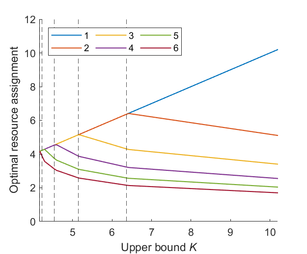
Figure 1: Optimal allocation decisions (each line corresponds to an individual)

In Proposition 1, we show that $\nu_{\bm{w}}(\bm{u})$ satisfies a set of basic axioms discussed in Section 3.

Proposition 1.

For any $\bm{w}\in\mathcal{W}$, the order-based inequity measure $\nu_{\bm{w}}:\mathbb{R}^{N}\rightarrow\mathbb{R}$ defined as $\nu_{\bm{w}}(\bm{u})=\sum_{i=1}^{N}w_{i}u_{(i)}$ satisfies Axioms C, N, S, SCV, TI, and PH.

Note that our order-based inequity measure resembles the form of the so-called ordered weighted average (OWA) operator (Csiszar, 2021; Yager, 1988) or the ordered median function (Nickel and Puerto, 2006). However, our order-based inequity measure differs from these operators in the following aspects. First, the OWA operator (and order-median function) takes the form $F_{\widetilde{\bm{w}}}(\bm{u})=\sum_{i=1}^{N}\widetilde{w}_{i}u_{(i)}$, where the weight vector $\widetilde{\bm{w}}\in\mathbb{R}^{N}$ satisfies $\widetilde{w}_{i}\in[0,1]$ and $\sum_{i=1}^{N}\widetilde{w}_{i}=1$. In contrast, the weight vector $\bm{w}\in\mathbb{R}_{\uparrow}^{N}$ in our order-based inequity measure satisfies $\sum_{i=1}^{N}w_{i}=0$ with $w_{1}<0$ and $w_{N}>0$ (see Definition 4.1). Second, as detailed in Yager (1988), the OWA operator is a way to aggregate different values of $u_{i}$, which was designed for multi-criteria decision-making problems and not for measuring inequity. Indeed, if $\widetilde{\bm{w}}\in\mathbb{R}_{\uparrow}^{N}$, which is a common assumption in the literature (see, e.g., Blanco et al., 2016; Nickel and Puerto, 2006; Rodríguez-Chía et al., 2000), then we can write $F_{\widetilde{\bm{w}}}$ as $F_{\widetilde{\bm{w}}}(\bm{u})=f(\bm{u})+\nu_{\bm{w}}(\bm{u})$, where $f(\bm{u})=N^{-1}\sum_{j=1}^{N}u_{j}$ and $\bm{w}=\widetilde{\bm{w}}-N^{-1}\bm{1}$. Here, $\nu_{\bm{w}}$ is an order-based inequity measure when $\widetilde{\bm{w}}\neq N^{-1}\bm{1}$. Thus, $F_{\bm{w}}$ (OWA) can be viewed as a special case of the general problem defined in (2) with a specific choice of the inefficiency measure $f(\bm{u})=N^{-1}\sum_{j=1}^{N}u_{j}$ (mean of $\bm{u})$ and the inequity measure $\nu_{\bm{w}}(\bm{u})$. In contrast, our framework allows adopting any classical inefficiency measure $f(\bm{u})$ in (2).

Next, in Theorem 1, we show that $\nu_{\bm{w}}$ is a supremum of linear functions (in $\bm{u}$) over a set of permutations of $\bm{w}$. As we show in Section 6, this characterization facilitates a unified reformulation of equity-promoting optimization models with order-based inequity measures.

Theorem 1.

Let $\Pi$ be the set of permutation functions $\pi:\mathbb{R}^{N}\rightarrow\mathbb{R}^{N}$ on $[N]$. For any $\bm{u}\in\mathbb{R}^{N}$, we have $\nu_{\bm{w}}(\bm{u})=\sup_{\widetilde{\bm{w}}\in\widetilde{\mathcal{W}}}\sum_{i=1}^{N}\widetilde{w}_{i}u_{i}$, where $\widetilde{\mathcal{W}}=\big{\{}\widetilde{\bm{w}}\in\mathbb{R}^{N}\mid\widetilde{w}_{i}=w_{\pi(i)},\,i\in[N],\,\pi\in\Pi\big{\}}$.

We now derive an axiomatic characterization of order-based inequity measures, i.e., a set of properties that characterize order-based inequity measures. First, the following axiom provides a practical mechanism to quantify the change in the value of the order-based inequity measure incurred by perturbation in the outcome (impact) vector $\bm{u}$.

Axiom PA (Proportional Adjustment).

There exist constants $\{w_{j}\}_{j\in[N]}$ such that $\phi(\bm{u}+\varepsilon\bm{e}_{j})=\phi(\bm{u})+\varepsilon w_{j}$ for any $\bm{u}\in\mathbb{R}_{\uparrow}^{N}$, $j\in[N]$, and $\varepsilon\in[0,u_{j+1}-u_{j}]$, where $[0,u_{N+1}-u_{N}]=[0,\infty)$.

Axiom PA has the following practical interpretation. Suppose we increase the $j$th smallest entry $u_{(j)}$ by a small amount $\varepsilon$. Then, the associated change in the value of the order-based inequity measure is proportional to $\varepsilon$. Mathematically, Axiom PA implies that $\phi(\bm{u}^{\prime})=\phi(\bm{u})+\sum_{j=1}^{N}w_{j}(u^{\prime}_{j}-u_{j})$ for any perturbation $\bm{u}^{\prime}\in\mathbb{R}^{N}$ of the vector $\bm{u}\in\mathbb{R}^{N}$ such that the order of each subject is preserved. Thus, Axiom PA characterizes the linearity of the order-based inequity measure with respect to $(u_{(1)},\dots,u_{(N)})^{\top}$. It follows that the effect of a change in the impact $u_{j}$ of subject $j$ depends only on the order (i.e., rank) of that subject, irrespective of the value of the impact (see Mehran, 1976 for similar discussions). In Theorem 2, we provide an axiomatic characterization of order-based inequity measures.

Theorem 2.

The function $\nu:\mathbb{R}^{N}\rightarrow\mathbb{R}$ is an order-based inequity measure with weight vector $\bm{w}\in\mathcal{W}$ if and only if $\nu$ satisfies Axioms N, SCV, PH, and PA.

Among the set of popular measures listed in Table 1, only measures (i)–(iii) are order-based (see Remark 5), where measure (i) is equivalent to measure (iii) (see A). In the following examples, we show how one can apply Theorem 2 to provide axiomatic characterizations of these order-based inequity measures, namely (i) and (ii).

Example 4.2 (Range).

Since $\max_{i\in[N]}u_{i}-\min_{i\in[N]}=-u_{(1)}+u_{(N)}$, it follows that the range is an order-based inequity measure with weight vector $\bm{w}^{\prime}:=(-1,0,\dots,0,1)^{\top}\in\mathbb{R}^{N}$. By Theorem 2, we have that Axioms N, SCV, PH, and PA with $\bm{w}=\bm{w}^{\prime}$ characterize the range. Specifically, Axiom PA with $\bm{w}=\bm{w}^{\prime}$ implies (a) there exists constant $C>0$ such that $\phi(\bm{u}+\varepsilon\bm{e}_{1})=\phi(\bm{u})-\varepsilon C$ for all $\varepsilon\in[0,u_{2}-u_{1}]$ and $\phi(\bm{u}+\varepsilon\bm{e}_{N})=\phi(\bm{u})+\varepsilon C$ for all $\varepsilon\geq 0$; (b) for all $j\in[2,N-1]$, $\phi(\bm{u}+\varepsilon\bm{e}_{j})=\phi(\bm{u})$ for all $\varepsilon\in[0,u_{j+1}-u_{j}]$. This indicates that the inequity measure’s value decreases (resp. increases) by a constant if the smallest (resp. largest) entry of $\bm{u}$ increases by a small amount $\varepsilon$, and it remains unchanged otherwise. This reflects the nature of the range that its value depends only on the value of the smallest ($u_{(1)}$) and largest ($u_{(N)}$) entries of $\bm{u}$.

Example 4.3 (Gini Deviation).

We can rewrite Gini deviation as $\sum_{i=1}^{N}\sum_{j=1}^{N}|u_{i}-u_{j}|=\sum_{i=1}^{N}2(2i-1-N)u_{(i)}=\sum_{i=1}^{N}w^{\prime}_{i}u_{(i)}$, where $w^{\prime}_{i}=2(2i-1-N)$ (Mesa et al., 2003). It is easy to verify that $\bm{w}^{\prime}\in\mathcal{W}$ (see Definition 4.1), i.e., Gini deviation is an order-based inequity measure with weight vector $\bm{w}^{\prime}$. By Theorem 2, we have that Axioms N, SCV, PH, and PA with $\bm{w}=\bm{w}^{\prime}$ characterize Gini deviation. Specifically, Axiom PA with $\bm{w}=\bm{w}^{\prime}$ implies that there exists constant $C>0$ such that $\phi(\bm{u}+\varepsilon\bm{e}_{j})=\phi(\bm{u})+\varepsilon C(2j-N-1)$ for any $\bm{u}\in\mathbb{R}_{\uparrow}^{N}$, $j\in[N]$, and $\varepsilon\in[0,u_{j+1}-u_{j}]$. Thus, if we increase the $j$th smallest entry $u_{(j)}$ by a small amount $\varepsilon$, the change in inequity measure’s value is proportional to $\varepsilon$ and scales linearly in $j$. In particular, if we increase $u_{(j)}$ for any $j\in[\lfloor(N-1)/2\rfloor]$, the inequity measure’s value decreases since $2j-N+1<0$, and the decrease is the most pronounced when we increase the smallest entry ($u_{(1)}$).

5 Convex Inequity Measures

In this section, we introduce our proposed class of convex inequity measures. We also derive a unified dual representation of convex inequity measures. Specifically, we show that one can equivalently represent any absolute convex inequity measure as a robustified order-based inequity measure over a set of weights $\bm{w}$ (Theorem 3). In addition to providing a unified mathematical expression of convex inequity measures, we show that this dual representation provides a mechanism to investigate the equivalence of convex inequity measures from a geometric perspective (Theorem 4). Finally, we use this dual representation in Section 6 to propose a unified framework for optimization models with a convex inequity measure.

In Section 5.1, we introduce the class of absolute convex inequity measures and discuss its properties. Then, in Section 5.2, we introduce the relative counterpart of absolute convex inequity measures and discuss their properties.

5.1 Absolute Convex Inequity Measure

We are now ready to introduce the class of absolute convex inequity measures.

Definition 5.1.

An inequity measure $\nu:\mathbb{R}^{N}\rightarrow\mathbb{R}$ is an absolute convex inequity measure if it satisfies Axioms C, N, S, TI, PH, and the following Axiom CV.

Axiom CV (Convexity).

$\phi\big{(}\alpha\bm{u}^{1}+(1-\alpha)\bm{u}^{2}\big{)}\leq\alpha\phi(\bm{u}^{1})+(1-\alpha)\phi(\bm{u}^{2})$ for any $\{\bm{u}^{1},\bm{u}^{2}\}\subset\mathbb{R}^{N}$ and $\alpha\in(0,1)$.

Convexity is a desirable mathematical property of inequity measure for use in optimization contexts. In particular, introducing a convex inequity measure to an optimization model does not generally pose an additional optimization burden compared with a non-convex inequity measure. In addition, as pointed out by Williamson and Menon (2019), if an inequity measure is non-convex, its value could be decreased by partitioning the subjects or groups of interests into subgroups, which is counter to what we wish to achieve (see also Kolm, 1976 for a thorough discussion). Specifically, if the inequity measure $\phi$ satisfies Axioms CV and PH, then $\phi$ is subadditive, i.e., $\phi(\bm{u}^{1}+\bm{u}^{2})\leq\phi(\bm{u}^{1})+\phi(\bm{u}^{2})$. On the other hand, if $\phi$ is not convex, then $\phi$ may not be subadditive, i.e., $\phi(\bm{u}^{1}+\bm{u}^{2})>\phi(\bm{u}^{1})+\phi(\bm{u}^{2})$. This implies that the inequity measure value would be smaller by dividing subjects into subgroups, which is undesirable.

Next, in Theorem 3, we provide one of the key results of this paper, which shows that any absolute convex inequity measure admits a dual representation as a worst-case order-based inequity measure over its dual set.

Theorem 3.

Consider an inequity measure $\nu:\mathbb{R}^{N}\rightarrow\mathbb{R}$, and let $\mathcal{S}^{N}=\{\bm{w}\in\mathbb{R}_{\uparrow}^{N}\mid\bm{1}^{\top}\bm{w}=0\}$. The following statements are equivalent: (a) $\nu$ is an absolute convex inequity measure; (b) there exists a convex compact set $\mathcal{W}_{\nu}\subseteq\mathcal{S}^{N}$ with $\mathcal{W}_{\nu}\neq\{\bm{0}\}$ such that $\nu(\bm{u})=\sup_{\bm{w}\in\mathcal{W}_{\nu}}\nu_{\bm{w}}(\bm{u})$; (c) there exists a compact set $\mathcal{W}_{\nu}\subseteq\mathcal{S}^{N}$ with $\mathcal{W}_{\nu}\neq\{\bm{0}\}$ such that $\nu(\bm{u})=\sup_{\bm{w}\in\mathcal{W}_{\nu}}\nu_{\bm{w}}(\bm{u})$.

Theorem 3 provides a dual representation of any absolute convex inequity measures characterized by a dual set, i.e., $\mathcal{W}_{\nu}\subseteq\{\bm{w}\in\mathbb{R}_{\uparrow}^{N}\mid\bm{1}^{\top}\bm{w}=0\}$. Specifically, it shows that any absolute convex inequity measure can be equivalently expressed as a robustified order-based inequity measure (i.e., worst-case over the dual set $\mathcal{W}_{\nu}$). Note that the dual set may not be unique in the sense that $\nu$ can equal $\sup_{\bm{w}\in\mathcal{W}_{1}}\nu_{\bm{w}}$ and $\sup_{\bm{w}\in\mathcal{W}_{2}}\nu_{\bm{w}}$ but $\mathcal{W}_{1}\neq\mathcal{W}_{2}$ (see Remark 4). Hence, due to the existence of multiple weight vectors in $\mathcal{W}_{\nu}$, absolute convex inequity measures are generally non-linear in $(u_{(1)},\dots,u_{(N}))^{\top}$. This is in contrast to the order-based inequity measures, which are linear in $(u_{(1)},\dots,u_{(N}))^{\top}$ as characterized by Axiom PA. Finally, Theorem 3 implies that one can construct any absolute convex inequity measure by defining a dual set. In particular, when preference information on $\bm{w}$ is incomplete or ambiguous, one can construct a set of potential weight vectors (i.e., the dual set) instead of using a single (biased) weight vector. This is useful in practice where the decision-maker is concerned about equity but cannot articulate her/his preference on $\bm{w}$ (see Armbruster and Delage, 2015; Hu et al., 2018 for similar discussions in preference robust optimization).

Remark 3.

Note that $\nu^{*}(\bm{0})=\sup_{\bm{u}\in\mathbb{R}^{N}}\big{\{}\bm{u}^{\top}\bm{0}-\nu(\bm{u})\big{\}}=-\inf_{\bm{u}\in\mathbb{R}^{N}}\nu(\bm{u})=0$, which implies that $\bm{0}\in\operatorname{dom}(\nu^{*})$.

Remark 4.

Let $\widetilde{\mathcal{W}}\subseteq\mathbb{R}^{N}$ be a compact set and consider the absolute convex inequity measure $\nu(\bm{u})=\sup_{\bm{w}\in\widetilde{\mathcal{W}}}\nu_{\bm{w}}(\bm{u})$. Then, $\nu(\bm{u})=\sup_{\bm{w}\in\operatorname{conv}(\widetilde{\mathcal{W}})}\nu_{\bm{w}}(\bm{u})$. Indeed, letting $\mathcal{P}$ be the set of permutation matrices, we have

$$\sup_{\bm{w}\in\widetilde{\mathcal{W}}}\nu_{\bm{w}}(\bm{u})=\sup_{\bm{w}\in\widetilde{\mathcal{W}}}\sup_{P\in\mathcal{P}}\bm{u}^{\top}(P\bm{w})=\sup_{P\in\mathcal{P}}\sup_{\bm{w}\in\widetilde{\mathcal{W}}}(P^{\top}\bm{u})^{\top}\bm{w}=\sup_{P\in\mathcal{P}}\sup_{\bm{w}\in\operatorname{conv}(\widetilde{\mathcal{W}})}(P^{\top}\bm{u})^{\top}\bm{w},$$

where the first equality follows from Theorem 1 and the last equality follows from the linearity of the objective.

Note that the dual set $\mathcal{W}_{\nu}$ characterizing an absolute convex inequity measure may have infinite weight vectors and thus may pose optimization burdens. However, in Proposition 2, we show that it suffices to consider only the non-zero extreme points of $\mathcal{W}_{\nu}$. Such characterization could help establish theoretical convergence guarantees of solution approaches that exploit the extreme points of the dual set $\mathcal{W}_{\nu}$ when solving optimization problems that involve an absolute convex inequity measure. We propose such an algorithm and discuss its convergence in Section 6.

Proposition 2.

Let $\nu$ be an absolute convex inequity measure with a convex dual set $\mathcal{W}_{\nu}$. Then, $\nu(\bm{u})=\sup_{\bm{w}\in\mathcal{E}(\mathcal{W}_{\nu})\setminus\{\bm{0}\}}\nu_{\bm{w}}(\bm{u})$, where $\mathcal{E}(\mathcal{W}_{\nu})$ is the set of extreme points of $\mathcal{W}_{\nu}$.

Since all the inequity measures in Table 1 are absolute convex inequity measures (see A), they admit the dual representation in Theorem 3. Next, in Proposition 3, we derive the dual sets of these inequity measures, which enable us to investigate the equivalence of these inequity measures from a geometric perspective (see Theorem 4 and Example 5.1).

Proposition 3.

The dual sets of inequity measures in Table 1 are as follows.

• For (i) and (iii), $\mathcal{W}_{\nu}=\{(-1,0,\dots,0,1)\in\mathbb{R}^{N}\}$.

• For (ii), $\mathcal{W}_{\nu}=\{\bm{w}^{\prime}\in\mathbb{R}^{N}\mid w^{\prime}_{i}=2(2i-1-N),\,\forall i\in[N]\}$.

• For (iv)–(vi), $\mathcal{W}_{\nu}=\{\bm{w}\in\mathbb{R}^{N}\mid\bm{w}=\bm{w}^{\prime}-\overline{w}^{\prime}\bm{1},\,\overline{w}^{\prime}=(1/N)\sum_{j=1}^{N}w^{\prime}_{j},\,\lVert\bm{w}^{\prime}\rVert_{q}\leq 1,\,\bm{w}^{\prime}\in\mathbb{R}_{\uparrow}^{N}\}$, where $q=\infty$, $q=2$, and $q=1$ for (iv), (v), and (vi), respectively.

• For (vii), $\mathcal{W}_{\nu}=\{\bm{w}\in\mathbb{R}^{N}\mid\bm{w}=\bm{w}^{\prime}-\overline{w}^{\prime}\bm{1},\,\overline{w}^{\prime}=(1/N)\sum_{j=1}^{N}w^{\prime}_{j},\,\lVert\bm{w}^{\prime}\rVert_{1}\leq N,\,\bm{w}^{\prime}\in\mathbb{R}_{\uparrow}^{N}\}$.

• For (viii), $\mathcal{W}_{\nu}=\{\bm{w}\in\mathbb{R}^{N}\mid w_{1}=-(N-k)-1,\,w_{2}=\dots=w_{k}=-1,\,w_{k+1}=\dots=w_{N-1}=1,\,w_{N}=k+1,\,k\in[N]\}$.

Remark 5.

It follows from Proposition 3 that measures (i)–(iii) are order-based since the dual sets of measures (i)–(iii) have only one weight vector satisfying Definition 4.1. Specifically, measures (i) and (iii) are order-based with $\bm{w}=(-1,0,\dots,0,1)\in\mathbb{R}^{N}$ and metric (ii) is order-based with $\bm{w}^{\prime}$, where $w^{\prime}_{i}=2(2i-1-N)$ for all $i\in[N]$. However, dual sets of measures (iv)–(viii) consist of more than one non-zero extreme point, and hence, (iv)–(viii) do not satisfy Definition 4.1, i.e., (iv)–(viii) are not order-based.

Next, in Theorem 4, we show that one can use the dual representation in Theorem 3 to verify whether two absolute convex inequity measures are equivalent. Here, we say two inequity measures $\nu^{1}$ and $\nu^{2}$ are equivalent if there exists $\beta>0$ such that $\nu^{1}(\bm{u})=\beta\nu^{2}(\bm{u})$ for all $\bm{u}\in\mathbb{R}^{N}$. Hence, replacing $\nu^{2}$ with $\nu^{1}$ (i.e., from $\nu^{2}$ to $\beta\nu^{2}$) in the equity-promoting optimization problem (2) or (3), essentially scales the weight on the equity criterion $\gamma$ or the upper bound $\eta$ by a factor of $\beta>0$.

Theorem 4.

Let $\nu_{1}$ and $\nu_{2}$ be two absolute convex inequity measures with dual sets $\mathcal{W}_{1}=\operatorname{dom}(\nu_{1}^{*})\cap\mathbb{R}_{\uparrow}^{N}$ and $\mathcal{W}_{2}=\operatorname{dom}(\nu_{2}^{*})\cap\mathbb{R}_{\uparrow}^{N}$, respectively. Then, $\nu_{1}$ is equivalent to $\nu_{2}$ if and only if $\mathcal{W}_{1}=\beta\mathcal{W}_{2}$ for some $\beta>0$.

Theorem 4 provides a mechanism to investigate the equivalence of absolute convex inequity measures from a geometric perspective via their dual sets. For example, let us first consider the case when there are two individuals or groups of interests ($N=2$). By Remark 3, the dual set $\mathcal{W}_{\nu}=\operatorname{dom}(\nu^{*})\cap\mathbb{R}_{\uparrow}^{2}$ of any two-dimensional absolute convex inequity measure $\nu$ on $\mathbb{R}^{2}$ is a line segment joining $\bm{0}$ and a point on $\mathcal{S}^{2}:=\{\bm{w}\in\mathbb{R}_{\uparrow}^{2}\mid\bm{1}^{\top}\bm{w}=0\}$ as shown in Figure 2(a). Hence, the duals sets of absolute convex inequity measures when $N=2$ are proportional. It follows from Theorem 4 that all two-dimensional absolute convex inequity measures are equivalent (i.e., will yield solutions with the same impact on equity). On the other hand, when $N>2$, absolute convex inequity measures may not be equivalent (i.e., will yield different solutions varying impact on equity). To see this, let us consider the case when $N=3$. In this case, as shown in Figure 2(b), the set $\mathcal{S}^{3}$ is a surface. Since dual sets $\mathcal{W}_{\nu_{1}}\subseteq\ \mathcal{S}^{3}$ and $\mathcal{W}_{\nu_{2}}\subseteq\mathcal{S}^{3}$ of two absolute convex inequity measures $\nu_{1}$ and $\nu_{2}$ may not be proportional, the two measures may not be equivalent. We illustrate this in Example 5.1.

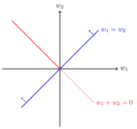
(a) Two dimensional (solid red line)

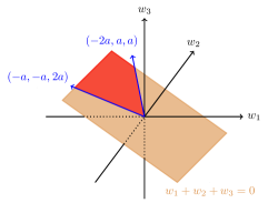
(b) Three dimensional (red surface)

Figure 2: Illustration of the set $\mathcal{S}^{N}=\{\bm{w}\in\mathbb{R}_{\uparrow}^{N}\mid\bm{1}^{\top}\bm{w}=0\}$ when (a) $N=2$ and (b) $N=3$

Example 5.1 (Dual sets in $\mathbb{R}^{3}$).

Figure 3 shows the dual sets for (iv)–(vi) when $N=3$. Note that the dual set of (iv) is proportional to that of (vi). Thus, by Theorem 4, (iv) and (vi) are equivalent. However, dual set of (v) has a curved boundary, implying that it is not proportional to that of (iv) and (vi). Thus, (v) is not equivalent to (iv) and (vi). These results are consistent with our algebraic proof of equivalence in A.

(a) Measure (iv)

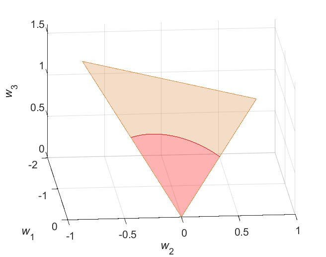
(b) Measure (v)

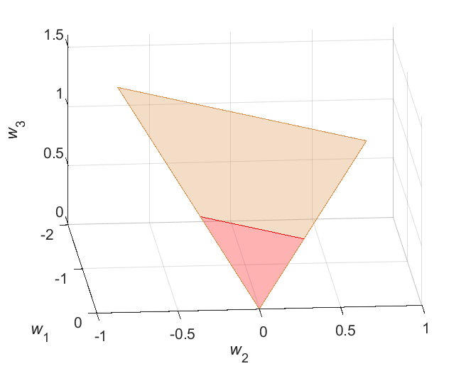
(c) Measure (vi)

Figure 3: Dual sets $\mathcal{W}_{\nu}$ (in red) of inequity measures (iv)–(vi) as subsets of $\mathcal{S}^{3}$ (in brown)

5.2 Relative Convex Inequity Measure

Recall that one can measure inequity in an absolute or relative sense. In this section, we build on our analyses of the absolute convex inequity measure proposed in Section 5.1 to introduce its relative counterpart and study its properties.

Definition 5.2.

Let $\nu:\mathbb{R}^{N}_{+}\rightarrow\mathbb{R}$ be an absolute convex inequity measure and $g:\mathbb{R}^{N}_{+}\rightarrow\mathbb{R}$ be a continuous function. An inequity measure $\rho:\mathbb{R}^{N}_{+}\rightarrow\mathbb{R}$ is a relative convex inequity measure if

$$\rho(\bm{u})=\frac{\nu(\bm{u})}{g(\bm{u})}$$ (5)

and $\rho$ satisfies Axioms S, SCV, SI, and the following Axiom NR. Here, we adopt the conventions $0/0=0$ and $a/0=\infty$ for any $a>0$.

Axiom NR (Normalization-Relative).

$\phi(\bm{u})\in[0,1]$ for any $\bm{u}\in\mathbb{R}_{+}^{N}$ and $\phi(\bm{u})=0$ if and only if $\bm{u}=\alpha\bm{1}$ for some $\alpha\in\mathbb{R}_{+}$.

We make a few remarks in order. First, we consider non-negative $\bm{u}$, which is common in many practical applications and consistent with prior studies (e.g., $\bm{u}$ could be patient waiting time, distances from demand nodes to open facilities, income, etc; see Ahmadi-Javid et al., 2017; Chakravarty, 1999; Marynissen and Demeulemeester, 2019; Mussard and Mornet, 2019; Pinedo, 2016). Second, Axiom NR is the relative counterpart of the normalization axiom discussed in Section 3. Specifically, we require that the relative convex inequity $\rho$ is normalized such that $\rho(\bm{u})\in[0,1]$ for any $\bm{u}\in\mathbb{R}^{N}_{+}$, which is consistent with the literature on relative inequity measures (Donaldson and Weymark, 1980; Mehran, 1976). In particular, with a suitable choice of $g$, we have that $\rho=0$ represents perfect equity while $\rho=1$ represents perfect inequity (see Proposition 4 and Corollary 1). Finally, since both $\nu$ and $g$ are continuous, $\rho$ is continuous on $\{\bm{u}\in\mathbb{R}_{+}^{N}\mid g(\bm{u})\neq 0\}$ by definition in (5). For example, if $g(\bm{u})=C\bm{1}^{\top}\bm{u}$ for some constant $C>0$, then $\rho(\bm{u})$ is continuous on $\mathbb{R}^{N}_{+}$ except at $\bm{u}=\bm{0}$ (see Theorem 6).

It is clear from the definition of $\rho$ in (5) that one should carefully choose the normalization function $g$ such that $\rho$ satisfies the desired set of axioms (i.e., NR, S, SCV, and SI). Hence, we next derive conditions and provide guidelines for choosing the normalization function $g$. First, in Theorem 5, we provide conditions on $g$ such that $\rho$ satisfies Axioms NR, S, and SI.

Theorem 5.

Let $\nu:\mathbb{R}^{N}_{+}\rightarrow\mathbb{R}$ be an absolute convex inequity measure and $g:\mathbb{R}^{N}_{+}\rightarrow\mathbb{R}$ be a continuous function. Then, the relative convex inequity measure $\rho=\nu/g$ satisfies Axioms NR, S, and SI if and only if $g$ is symmetric and positive homogeneous with $g\geq\nu$.

Theorem 5 provides sufficient and necessary conditions on $g$ for which the relative convex inequity measure $\rho$ satisfies Axioms NR, S, and SI. Specifically, $g$ belongs to the class of continuous and positive homogeneous functions with $g\geq\nu$. Note that although the absolute convex inequity measure $\nu$ is Schur convex, the relative counterpart might not. Thus, in addition to Theorem 5, we need to impose conditions on the normalization function $g$ to ensure that $\rho$ is Schur convex. Theorem 6 provides a sufficient condition on $g$ such that $\rho$ is Schur convex, and hence, satisfies Definition 5.2.

Theorem 6.

Let $\nu:\mathbb{R}^{N}_{+}\rightarrow\mathbb{R}$ be an absolute convex inequity measure and $g:\mathbb{R}^{N}_{+}\rightarrow\mathbb{R}$ be a continuous function. If $g(\bm{u})=CN\overline{u}$ with $\overline{u}=N^{-1}\sum_{i=1}^{N}u_{i}$ for any $C\geq\sup_{\bm{w}\in\mathcal{W}_{\nu}}\lVert\bm{w}\rVert_{\infty}$, then the relative convex inequity measure $\rho=\nu/g$ satisfies Axioms NR, S, SCV, and SI.

Let us provide an intuitive justification for choosing $g(\bm{u})=CN\overline{u}$ as suggested by Theorem 6. Let $\bm{u}\in\mathbb{R}^{N}_{+}$ with $\bm{1}^{\top}\bm{u}=\gamma>0$, i.e., the total impact on the $N$ subjects is $\gamma$. Suppose that we can re-distribute the $\gamma$ units of impact among the subjects. Then, $\bm{u}_{\text{min}}=\gamma/N\cdot\bm{1}$ minimizes $\nu$ with $\nu_{\text{min}}=\nu(\bm{u}_{\text{min}})=0$, and $\bm{u}_{\text{max}}=(0,\dots,0,\gamma)^{\top}$ maximizes $\nu$ with $\nu_{\text{max}}=\nu(\bm{u}_{\text{max}})=\gamma\sup_{\bm{w}\in\mathcal{W}_{\nu}}\lVert\bm{w}\rVert_{\infty}$. Thus, an intuitive way to normalize $\nu(\bm{u})$ such that $0\leq\rho(\bm{u})\leq 1$ is as follows:

$$\frac{\nu(\bm{u})-\nu_{\text{min}}}{\nu_{\text{max}}-\nu_{\text{min}}}=\frac{\nu(\bm{u})}{\gamma\sup_{\bm{w}\in\mathcal{W}_{\nu}}\lVert\bm{w}\rVert_{\infty}}=\frac{\nu(\bm{u})}{\bm{1}^{\top}\bm{u}\cdot\sup_{\bm{w}\in\mathcal{W}_{\nu}}\lVert\bm{w}\rVert_{\infty}}=\frac{\nu(\bm{u})}{(N\sup_{\bm{w}\in\mathcal{W}_{\nu}}\lVert\bm{w}\rVert_{\infty})\cdot\overline{u}}.$$ (6)

The denominator in (6) takes the same form of $g$ suggested in Theorem 6. Indeed, it is also common in the existing literature to normalize an absolute inequity measure by a function of the mean $\overline{u}$ of $\bm{u}$ (Chakravarty, 1999; Mussard and Mornet, 2019; Zheng, 2007).

Next, in Theorem 7, we show that if we restrict the normalization function $g$ to be a function of the mean $\overline{u}$, then $g(\bm{u})$ can only take the following form $g(\bm{u})=CN\overline{u}$, i.e., a necessary condition on $g$ for $\rho$ to be a relative convex inequity measure satisfying Definition 5.2. Note that there are no general necessary conditions on $g$ for the relative convex inequity measure $\rho$ to be Schur convex. For example, $\rho$ can be Schur convex even for some non-convex and non-concave $g$ (see C).

Theorem 7.

Let $\nu:\mathbb{R}^{N}_{+}\rightarrow\mathbb{R}$ be an absolute convex inequity measure and $g:\mathbb{R}^{N}_{+}\rightarrow\mathbb{R}$ be a continuous function. Suppose that $g(\bm{u})=\tilde{g}(\overline{u})$ is a function of mean $\overline{u}=N^{-1}\sum_{i=1}^{N}u_{i}$ of $\bm{u}$. Then, the relative convex inequity measure $\rho=\nu/g$ satisfies Axioms NR, S, SCV, and SI if and only if $\tilde{g}(\overline{u})=CN\overline{u}$ for any $C\geq\sup_{\bm{w}\in\mathcal{W}_{\nu}}\lVert\bm{w}\rVert_{\infty}$.

Theorem 7 shows that if the normalization function $g$ is a function of the mean $\overline{u}$, then a linear function in $\overline{u}$ is the only possible choice such that $\rho$ satisfies Axioms NR, S, SCV, and SI. We can also see from (6) that $g(\bm{u})=CN\overline{u}$ with $C=\sup_{\bm{w}\in\mathcal{W}_{\nu}}\lVert\bm{w}\rVert_{\infty}$ is an intuitive choice.

Observe from (6) that $\rho(\bm{u})=0$ when the absolute convex inequity measure attains its minimum value of zero, i.e., $\nu(\bm{u})=\nu(\bm{u}_{\text{min}})=0$, where $\bm{u}_{\text{min}}\in\operatorname*{arg\,min}\{\nu(\bm{u})\mid\bm{1}^{\top}\bm{u}=\gamma\}$ for any $\gamma>0$. Thus, like other relative inequity measures in the literature, $\rho(\bm{u})=0$ implies perfect equity (Axiom NR). On the other hand, $\rho(\bm{u})$ attains its maximum value of one when the absolute convex inequity measure attains its maximum value, i.e., $\nu(\bm{u})=\nu(\bm{u}_{\text{max}})$, where $\bm{u}_{\text{max}}\in\operatorname*{arg\,max}\{\nu(\bm{u})\mid\bm{1}^{\top}\bm{u}=\gamma\}$ for any $\gamma>0$. It follows that $\rho(\bm{u})=1$ indicates perfect inequity. We formalize the latter observation in Proposition 4.

Proposition 4.

Let $\nu$ be an absolute convex inequity measure and $g(\bm{u})=\sup_{\bm{w}\in\mathcal{W}_{\nu}}\lVert\bm{w}\rVert_{\infty}N\overline{u}$ with $\overline{u}=N^{-1}\sum_{i=1}^{N}u_{i}$. Then, the relative convex inequity measure $\rho(\bm{u})=\nu(\bm{u})/g(\bm{u})=1$ if and only if $\bm{u}\in\mathcal{U}^{\star}=\bigcup_{\gamma>0}\mathcal{U}^{\star}_{\gamma}$, where $\mathcal{U}^{\star}_{\gamma}=\operatorname*{arg\,max}_{\bm{u}^{\prime}}\{\nu(\bm{u}^{\prime})\mid\bm{1}^{\top}\bm{u}^{\prime}=\gamma\}$.

In Corollary 1, we show that under some additional mild assumption on $\nu$, the relative convex inequity measure achieves its maximum $\rho(\bm{u})=1$ if and only if $\bm{u}$ takes the form $P(0,\dots,0,\gamma)^{\top}\in\mathbb{R}^{N}$ for any $\gamma>0$ and permutation matrix $P$.

Corollary 1.

Let $\nu$ be an absolute convex inequity measure and $g(\bm{u})=\sup_{\bm{w}\in\mathcal{W}_{\nu}}\lVert\bm{w}\rVert_{\infty}N\overline{u}$ with $\overline{u}=N^{-1}\sum_{i=1}^{N}u_{i}$. Assume that $\nu(0,\dots,0,0,\gamma)>\nu(0,\dots,0,\gamma/2,\gamma/2)$ for any $\gamma>0$. Then, $\rho(\bm{u})=\nu(\bm{u})/g(\bm{u})=1$ if and only if $\bm{u}=P(0,\dots,0,\gamma)^{\top}$ for any $\gamma>0$ and permutation matrix $P$.

Remark 6.

Note that the constant $w_{\text{max}}=\sup_{\bm{w}\in\mathcal{W}_{\nu}}\lVert\bm{w}\rVert_{\infty}$ can be computed directly without solving the supremum problem. Specifically, since $\nu(\bm{u})=\sup_{\bm{w}\in\mathcal{W}\nu}\nu_{\bm{w}}(\bm{u})$ (see Theorem 3), we have $\nu(0,\dots,0,\gamma)=\gamma w_{\text{max}}$, which implies $w_{\text{max}}=\nu(0,\dots,0,\gamma)/\gamma$ for any $\gamma>0$.

We close this section with Example 5.2, where we derive the relative counterparts of the deviation-based inequity measures in Table 1 and make connections to existing relative inequity measures.

Example 5.2 (Relative counterparts of the inequity measures in Table 1).

a

1. Recall that measure (i) is order-based with $\bm{w}=(-1,0,\dots,0,1)$. Thus, we have $w_{\text{max}}=1$, and hence,

   $$\rho(\bm{u})=\frac{\nu(\bm{u})}{N\overline{u}}=\frac{u_{(N)}-u_{(1)}}{N\overline{u}},$$

   which is equivalent to the relative range (Cowell, 2011). Note that (iii) is equivalent to (i) (see A). Thus, the relative counterpart of (iii) takes the same form as (i).

2. Recall that measure (ii) is order-based with $w_{i}=2(2i-N-1)$ for $i\in[N]$. Thus, we have $w_{\text{max}}=2(N-1)$, and hence,

   $$\rho(\bm{u})=\frac{\nu(\bm{u})}{2N(N-1)\overline{u}}=\frac{\sum_{i\in[N]}\sum_{j\in[N]}|u_{i}-u_{j}|}{2N(N-1)\overline{u}},$$

   which is equivalent to the Gini index (Gini, 1912).

3. For measure (iv), we have $w_{\text{max}}=\nu(0,\dots,0,\gamma)/\gamma=2[1-(1/N)]$, and hence,

   $$\rho(\bm{u})=\frac{\nu(\bm{u})}{2(N-1)\overline{u}}=\frac{\sum_{i\in[N]}|u_{i}-\overline{u}|}{2(N-1)\overline{u}},$$

   which is equivalent to the relative mean absolute deviation, also known as the Hoover index (Hoover, 1936).

4. For measure (v), we have $w_{\text{max}}=\nu(0,\dots,0,\gamma)=\sqrt{1-(1/N)}$, and hence,

   $$\rho(\bm{u})=\frac{\nu(\bm{u})}{\sqrt{N}\sqrt{N-1}\overline{u}}=\frac{\sqrt{(N-1)^{-1}\sum_{i\in[N]}(u_{i}-\overline{u})^{2}}}{\sqrt{N}\overline{u}},$$

   which is equivalent to the relative standard deviation or the coefficient of variation (Cowell, 2011).

5. For measure (vi), we have $w_{\text{max}}=\nu(0,\dots,0,\gamma)/\gamma=1-(1/N)$, and hence,

   $$\rho(\bm{u})=\frac{\nu(\bm{u})}{(N-1)\overline{u}}=\frac{\max_{i\in[N]}|u_{i}-\overline{u}|}{(N-1)\overline{u}}.$$

   Note that measure (vii) is equal to $N$ times measure (vi) (see A). Thus, the relative counterpart of (vii) takes the same form as (vi).

6. For measure (viii), we have $w_{\text{max}}=\nu(0,\dots,0,\gamma)/\gamma=N$, and hence,

   $$\rho(\bm{u})=\frac{\nu(\bm{u})}{N^{2}\overline{u}}=\frac{\sum_{i\in[N]}\max_{j\in[N]}|u_{i}-u_{j}|}{N^{2}\overline{u}}.$$

6 Optimization with Convex Inequity Measures

In this section, we propose solution approaches to solve optimization problems with our proposed convex inequity measures. Specifically, we focus on equity-promoting optimization models of the form (2), where the inequity measure is incorporated into the objective function. As mentioned in Section 3, relative inequity measures might be more appropriate for problems of the form (3); thus, we focus on absolute convex inequity measures in this section. In D, we show how one can leverage the proposed approaches to solve equity-promoting problems of the form (3) using absolute or relative convex inequity measures.

Our proposed solution approaches can be used to solve problem (2) with any inefficiency measure $f$ (see Examples 6.1 and 6.2). However, for notational convenience and ease of exposition, we focus on the optimization problem

$$\min_{\bm{x},\,\bm{u}}\Big{\{}\nu(\bm{u})\,\Big{|}\,\bm{u}=U(\bm{x}),\,\bm{x}\in\mathcal{X}\Big{\}}.$$ (7)

In Section 6.1, we derive unified reformulations of (7) when $\nu$ is an order-based inequity measure. Then, in Section 6.2, we propose an decomposition algorithm to solve (7) when $\nu$ is an absolute convex inequity measure. We also provide numerical examples demonstrating the computational efficiency of our proposed approach over existing ones.

6.1 Minimizing Order-based Inequity Measures

We first consider problem (7) with an order-based inequity measure objective $\nu_{\bm{w}}$ for some $\bm{w}\in\mathcal{W}$ (see Section 4). First, in Theorem 8, we use the characterization of $\nu_{\bm{w}}$ in Theorem 1 to derive an equivalent reformulation of problem (7) with $\nu=\nu_{\bm{w}}$.

Theorem 8.

Problem (7) with an order-based inequity measure $\nu_{\bm{w}}$ is equivalent to

$$\underset{\bm{x},\,\bm{u},\,\bm{\lambda}\in\mathbb{R}^{N},\,\bm{\theta}\in\mathbb{R}^{N}}{\textup{minimize}\,}\quad \bm{1}^{\top}(\bm{\lambda}+\bm{\theta})$$ (8a)

subject to $$\lambda_{i}+\theta_{j}\geq u_{i}w_{j},\quad\forall i\in[N],\,j\in[N],$$ (8b)

$$\bm{u}=U(\bm{x}),\,\bm{x}\in\mathcal{X}.$$ (8c)

We make two remarks in order. First, formulation (8) is linear if $U$ is linear and $\mathcal{X}$ is a set of linear constraints on $\bm{x}$. Second, variables $\bm{\lambda}$ and $\bm{\theta}$ in (8) are unrestricted in sign. In Proposition 5, we derive lower and upper bounds on $\bm{\lambda}$ and $\bm{\theta}$, which could reduce the search space of these variables.

Proposition 5.

Let $U_{\textup{max}}=\sup\limits_{\bm{x}\in\mathcal{X}}\max\limits_{i\in[N]}[U(\bm{x})]_{i}$ and $U_{\textup{min}}=\inf\limits_{\bm{x}\in\mathcal{X}}\min\limits_{i\in[N]}[U(\bm{x})]_{i}$, where $[U(\bm{x})]_{i}$ is the $i$th entry of $U(\bm{x})$. Without loss of optimality, we can impose the following bounds on variables $\bm{\lambda}$ and $\bm{\theta}$ in (8). For all $i\in[N]$,

$$0 \leq\lambda_{i}\leq(U_{\textup{max}}-U_{\textup{min}})\lVert\bm{w}\rVert_{\infty}=:\overline{\lambda},$$ (9)

$$\min\big{\{}U_{\textup{max}}w_{i},\,U_{\textup{min}}w_{i}\big{\}}-\overline{\lambda} \leq\theta_{i}\leq\max\big{\{}U_{\textup{max}}w_{i},\,U_{\textup{min}}w_{i}\big{\}}.$$ (10)

In the following example, we use a facility location problem with inequity and classical inefficiency measures to show how our proposed reformulation provides computational gain over existing ones.

Example 6.1 (Gini deviation reformulation).

Consider the problem of minimizing the Gini deviation, i.e., $\sum_{i=1}^{N}\sum_{i^{\prime}=1}^{N}|u_{i}-u_{i}^{\prime}|$. Existing literature (Chen and Hooker, 2023; Lejeune and Turner, 2019; Shehadeh and Snyder, 2021) introduce auxiliary variables $z_{i,i^{\prime}}=|u_{i}-u_{i^{\prime}}|$ and use the following equivalent reformulation:

$$\min_{\bm{x},\,\bm{u},\,\bm{z}}\Bigg{\{}\sum_{i=1}^{N}\sum_{i^{\prime}=1}^{N}z_{i,i^{\prime}}\,\Bigg{|}\,z_{i,i^{\prime}}\geq u_{i}-u_{i^{\prime}},\,z_{i,i^{\prime}}\geq u_{i^{\prime}}-u_{i},\,\forall\{i,i^{\prime}\}\subseteq[N],\,\bm{u}=U(\bm{x}),\,\bm{x}\in\mathcal{X}\Bigg{\}}.$$ (11)

In addition to variables $(\bm{x},\bm{u})$ and the constraints in (7), this reformulation requires $N^{2}$ variables $\bm{z}$ and $N^{2}$ constraints on $\bm{z}$, while our reformulation (8) involves only $2N$ variables $(\bm{\lambda},\bm{\theta})$ and $N^{2}$ constraints on $(\bm{\lambda},\bm{\theta})$. Thus, our reformulation has a significantly smaller number of variables, especially when $N$ is large.

To illustrate the potential computational gains when using our reformulation in (8) instead of formulation (11), we consider a $p$-median facility location problem. Given a set of customer locations $I$ and potential facility locations $J$, we want to decide where to open $p<|J|$ facilities to minimize the sum of the total transportation cost (i.e., an efficiency measure) and the Gini deviation in the transportation cost across all customers. The demand at $i\in I$ is $d_{i}$ and the transportation cost, per unit demand, between $i\in I$ and $j\in J$ is $c_{ij}$. Let $x_{j}$ be a binary variable taking value $1$ if facility $j$ is open, and $y_{ij}$ be a binary variable taking value $1$ if customer $i$ is assigned to facility $j$, and are $0$ otherwise. Finally, we define a non-negative variable $r_{i}$ as the transportation cost of $i\in I$. With this notation, we formulate this problem as

$$\underset{\bm{x}\in\{0,1\}^{J},\,\bm{y}\in\{0,1\}^{I\times J},\,\bm{r}}{\textup{minimize}\,}\quad \gamma\sum_{i\in I}r_{i}+(1-\gamma)\nu(\bm{r})$$ (12a)

subject to $$r_{i}=\sum_{j\in J}d_{i}c_{ij}y_{ij},\quad\forall i\in I,$$ (12b)

$$\sum_{j\in J}x_{j}=p,\,\,\sum_{j\in J}y_{ij}=1,\,\,y_{ij}\leq x_{j},\quad\forall i\in I,\,j\in J,$$ (12c)

where (12c) ensures that only $p$ facilities are open, and each customer is assigned to exactly one open facility. For the objective, we use a convex combination of the total transportation cost and the Gini deviation $\nu(\bm{r})=|I|^{-1}\sum_{i\in I}\sum_{i^{\prime}\in I}|r_{i}-r_{i^{\prime}}|$.

We use data from Daskin (2013) to generate five random instances for each combination of $|I|\in\{40,50\}$ and $p\in\{|I|/3,|I|/4,|I|/5\}$, rounded to the nearest integer (see E for implementation details). We solve these instances using the linear reformulation (11) and our reformulation (8) with (9)–(10). Table 2 shows the minimum (min), average (avg), and maximum (max) computational time (in seconds) over five generated instances. In particular, we consider $\gamma=0.2$, where more emphasis is put on the inequity measure. It is clear from Table 2 that our reformulation can solve all the generated instances significantly faster. Moreover, when $|I|=50$ and $p=10$, we can solve all instances using our reformulation within 40 minutes, but we cannot solve these instances with (11) within 2 hours. These results demonstrate the computational advantages of our unified reformulation.

Table 2: Solution time (in seconds) over five randomly generated instances with $\gamma=0.2$. Note: Solution times with ‘$>$’ indicate that one or more instances cannot be solved within the imposed $2$-hour time limit.

	$p=13$			$p=10$			$p=8$
$|I|=40$	min	avg	max	min	avg	max	min	avg	max
Our Reformulation (8)	27	41	65	29	128	315	37	272	753
Linear Reformulation (11)	37	61	116	52	390	1299	50	1581	5778
	$p=17$			$p=13$			$p=10$
$|I|=50$	min	avg	max	min	avg	max	min	avg	max
Our Reformulation (8)	74	351	872	388	692	1062	1405	1833	2364
Linear Reformulation (11)	127	316	638	253	1439	2662	$>$7200	$>$7200	$>$7200

6.2 Minimizing Convex Inequity Measures

Let us now consider problem (7) with a convex inequity measure objective (see Section 5). By the dual representation in Theorem 3, we can reformulate problem (7) as

$$\quad\,\,\min_{\bm{x},\,\bm{u}}\bigg{\{}\sup_{\bm{w}\in\mathcal{W}_{\nu}}\nu_{\bm{w}}(\bm{u})\,\bigg{|}\,\bm{u}=U(\bm{x}),\,\bm{x}\in\mathcal{X}\bigg{\}}$$

$$=\min_{\bm{x},\,\bm{u},\,\delta}\bigg{\{}\delta\,\bigg{|}\,\delta\geq\textstyle\sum\limits_{i=1}^{N}w_{i}u_{(i)},\,\forall\bm{w}\in\mathcal{W}_{\nu},\,\bm{u}=U(\bm{x}),\,\bm{x}\in\mathcal{X}\bigg{\}}.$$ (13)

Problem (13) is challenging to solve because of the following two reasons. First, note that the order-based inequity measure $\nu_{\bm{w}}(\bm{u})=\sum_{i=1}^{N}w_{i}u_{(i)}$ is a function of the ordered entries of $\bm{u}$. Thus, the constraint $\delta\geq\sum_{i=1}^{N}w_{i}u_{(i)}$ is non-linear in $\bm{u}$. Second, $\mathcal{W}_{\nu}$ may not be finite, i.e., (13) is a semi-infinite program. However, from Proposition 2, we know that it suffices to consider the non-zero extreme points of the dual set $\mathcal{W}_{\nu}$ to solve problem (13). Leveraging this fact, we next propose a column-and-constraint generation algorithm (C&CG) to solve problem (13). Algorithm 1 summarizes the steps of our C&CG.

Initialization : Set $LB=0$, $UB=\infty$, $\varepsilon>0$, $j=1$, $\bm{w}^{0}\in\mathcal{W}_{\nu}$.

1. Master problem.

     Solve master problem (15) with weights $\{\bm{w}^{0},\dots,\bm{w}^{j-1}\}$.

     Record the optimal solution $(\bm{x}^{j},\bm{u}^{j})$ and optimal value $\delta^{j}$.

     Set $LB\leftarrow\max\{LB,\delta^{j}\}$.

2. Subproblem. Solve subproblem (16) for fixed $\bm{u}=\bm{u}^{j}$.

     Record the optimal solution $\bm{w}^{j}$ and value $D^{j}$. Set $UB\leftarrow\min\big{\{}UB,\,D^{j}\big{\}}$.

     If $(UB-LB)/UB<\varepsilon$, terminate and return the solution with best objective.

3. Scenario set enlargement.

     Update $j\leftarrow j+1$ and go back to step 1.

Algorithm 1 The column-and-constraint generation algorithm (C&CG)

In C&CG, we solve a master problem and subproblem at each iteration. Specifically, at iteration $j$ of C&CG, we aim to solve the following master problem

$$\min_{\bm{x},\,\bm{u},\,\delta}\bigg{\{}\delta\,\bigg{|}\,\delta\geq\textstyle\sum\limits_{i=1}^{N}w_{i}u_{(i)},\,\forall\bm{w}\in\{\bm{w}^{0},\dots,\bm{w}^{j-1}\},\,\bm{u}=U(\bm{x}),\,\bm{x}\in\mathcal{X}\bigg{\}},$$ (14)

where $\{\bm{w}^{0},\dots,\bm{w}^{j-1}\}\subseteq\mathcal{W}_{\nu}$. Note again that (14) is not directly solvable in the presented form due to the non-linearity of constraint $\delta\geq\sum_{i=1}^{N}w_{i}u_{(i)}$. However, in Proposition 6, we provide an equivalent solvable reformulation of (14).

Proposition 6.

The master problem (14) in C&CG is equivalent to

$$\underset{\bm{x},\,\bm{u},\,\bm{\lambda},\,\bm{\theta},\,\delta}{\textup{minimize}}\quad \delta$$ (15a)

subject to $$\delta\geq\bm{1}^{\top}(\bm{\lambda}^{k}+\bm{\theta}^{k}),\quad\forall k\in[0,j-1]_{\mathbb{Z}},$$ (15b)

$$\lambda^{k}_{i}+\theta^{k}_{i^{\prime}}\geq u_{i}w_{i^{\prime}}^{k},\quad\forall i\in[N],\,i^{\prime}\in[N],\,k\in[0,j-1]_{\mathbb{Z}},$$ (15c)

$$\bm{u}=U(\bm{x}),\,\bm{x}\in\mathcal{X}.$$ (15d)

Since only a set of weight vectors in $\mathcal{W}_{\nu}$ is considered, the master problem is a relaxation of the original problem (13), and thus its optimal value $\delta^{j}$ provides a lower bound to (13). With the optimal solution $\bm{u}^{j}$ from the master problem, we solve the following subproblem

$$D^{j}=\max\bigg{\{}\textstyle\sum\limits_{i=1}^{N}w_{i}u^{j}_{(i)}\,\bigg{|}\,\bm{w}\in\mathcal{W}_{\nu}\bigg{\}},$$ (16)

and record the optimal solution $\bm{w}^{j}\in\mathcal{W}_{\nu}$ of the subproblem. Since $\bm{u}^{j}$ obtained from the master problem is feasible, $D^{j}$ provides an upper bound to (13). Note that subproblem (16) is always feasible by construction because $\mathcal{W}_{\nu}$ is non-empty. Since $\mathcal{W}_{\nu}$ is convex (see Remark 4) and the objective $\sum_{i=1}^{N}w_{i}u_{(i)}$ is linear, subproblem (16) can be efficiently solved using convex optimization algorithms. In particular, if $\mathcal{W}_{\nu}$ is a polytope, subproblem (16) reduces to a linear program. Finally, if the gap between the lower and upper bounds is smaller than a pre-specified tolerance $\varepsilon$, C&CG terminates and returns the solution with the best objective value $UB$. Otherwise, we proceed to the next iteration and solve the master problem with an enlarged subset of weights $\{\bm{w}^{0},\dots,\bm{w}^{j}\}$. Note that one can set the initial weight $\bm{w}^{0}$ as the zero vector $\bm{0}$ (see Remark 3).

Next, we discuss the convergence of the proposed C&CG. Note that $\mathcal{W}_{\nu}$ is compact and convex. If, in addition, $\mathcal{X}$ is compact (a mild assumption that holds valid in a wide-range of applications, including facility location and scheduling problems; see Ahmadi-Javid et al., 2017; Celik Turkoglu and Erol Genevois, 2020; Marynissen and Demeulemeester, 2019), Proposition 2 of Bertsimas and Shtern (2018) ensures that any accumulation point of the sequence $\{\bm{x}^{j}\}_{j\in\mathbb{N}}$ generated from C&CG is an optimal solution to (13). Moreover, if $\mathcal{W}_{\nu}$ is a polyhedron and a vertex is always returned when solving the subproblem, C&CG terminates in a finite number of iterations by Proposition 2.

In the following example, we again use the $p$-median facility location problem to show how our proposed C&CG provides computational gain over existing ones.

Example 6.2 (Mean absolute deviation reformulation).

Consider the problem of minimizing the mean absolute deviation (MAD), i.e., $\sum_{i=1}^{N}|u_{i}-\overline{u}|$, where $\overline{u}=N^{-1}\sum_{i=1}^{N}$. Existing literature (Chen and Hooker, 2023; Shehadeh and Snyder, 2021) introduce auxiliary variables $z_{i}=|u_{i}-\overline{u}|$ and use the following equivalent reformulation:

$$\min_{\bm{x},\,\bm{u},\,\bm{z}}\Bigg{\{}\sum_{i=1}^{N}z_{i}\,\Bigg{|}\,z_{i}\geq u_{i}-\frac{1}{N}\sum_{i^{\prime}=1}^{N}u_{i^{\prime}},\,z_{i}\geq\frac{1}{N}\sum_{i^{\prime}=1}^{N}u_{i^{\prime}}-u_{i},\forall i\in[N],\,\bm{u}=U(\bm{x}),\,\bm{x}\in\mathcal{X}\Bigg{\}}.$$ (17)

On the other hand, from Proposition 3, we know that MAD is an absolute convex inequity measure with dual set $\mathcal{W}_{\nu}=\{\bm{w}\in\mathbb{R}^{N}\mid\bm{w}=\bm{w}^{\prime}-\overline{w}^{\prime}\bm{1},\,\overline{w}^{\prime}=(1/N)\sum_{j=1}^{N}w^{\prime}_{j},\,\lVert\bm{w}^{\prime}\rVert_{\infty}\leq 1,\,\bm{w}^{\prime}\in\mathbb{R}_{\uparrow}^{N}\}$. Thus, we could apply our proposed C&CG method to solve optimization problems with an MAD objective.

To illustrate the computational benefits of our proposed C&CG method over the classical reformulation, we conduct the same numerical experiment as in Example 6.1. Specifically, we solve (12) with $\nu(\bm{r})=\sum_{i=1}^{N}|r_{i}-\bar{r}|$, where $\bar{r}=N^{-1}\sum_{i=1}^{N}r_{i}$. Table 3 shows the minimum (min), average (avg), and maximum (max) computational time (in seconds) over five generated instances. It is clear that using our reformulation and the proposed C&CG, we can solve all the generated instances significantly faster than the classical reformulation technique. For example, when $|I|=40$, the solution time using our approach ranges from $17$ seconds to $35$ minutes while the solution time using (17) ranges from $32$ seconds to $2$ hours. When $|I|=50$, we can solve all instances using our approach, but we cannot solve most instances using (17) within $2$ hours. These results demonstrate the computational advantages of our unified reformulation and the proposed C&CG method over the classical linear reformulation.

Table 3: Solution time (in seconds) over five randomly generated instances with $\gamma=0.2$. Solution times with ‘$>$’ indicate that one or more instances cannot be solved within the imposed $2$-hour time limit.

	$p=13$			$p=10$			$p=8$
$|I|=40$	min	avg	max	min	avg	max	min	avg	max
C&CG Method	17	141	437	28	294	1030	75	738	1943
Linear Reformulation (17)	32	253	630	114	882	2745	136	3203	5765
	$p=17$			$p=13$			$p=10$
$|I|=50$	min	avg	max	min	avg	max	min	avg	max
C&CG Method	124	1339	4229	521	1107	2133	785	2539	5715
Linear Reformulation (17)	191	$>$3605	$>$7200	5330	$>$6834	$>$7200	$>$7200	$>$7200	$>$7200

7 Stability Analysis

Given that there are many different convex inequity measures, it is crucial to quantify how the choice of convex inequity measure in the objective of an optimization problem would affect the optimal value and solution. In this section, we leverage the dual representation of absolute convex inequity measures to investigate the stability of the optimal value and solution of the equity-promoting optimization problem of the form (2), i.e., $\min\big{\{}f(\bm{u})+\gamma\phi(\bm{u})\,\big{|}\,\bm{u}=U(\bm{x}),\,\bm{x}\in\mathcal{X}\big{\}}$, with respect to the choice of different absolute convex inequity measures in the objective. Note that replacing the inequity measure in the objective of problem (2) with another does not impact the feasibility of the problem. However, the optimal solution may differ if the two measures are not equivalent. In contrast, replacing the inequity measure in the constraints as in problem (3) (i.e., $\phi(\bm{u})\leq\eta$) with another one may impact the feasibility of the problem if the two measures are not equivalent due to the upper bound $\eta$ on the value of the inequity measure.

Let us first define the following additional notation used in the analysis. We define the distance between a point $\bm{w}\in\mathbb{R}^{N}$ and a set $\mathcal{W}$ as $d(\bm{w},\mathcal{W}):=\inf_{\widetilde{\bm{w}}\in\mathcal{W}}\lVert\bm{w}-\widetilde{\bm{w}}\rVert_{2}$, and the Hausdorff distance between two sets $\mathcal{W}_{1}$ and $\mathcal{W}_{2}$ as $d_{H}(\mathcal{W}_{1},\mathcal{W}_{2}):=\max\big{\{}\sup_{\bm{w}_{2}\in\mathcal{W}_{2}}d(\bm{w}_{2},\mathcal{W}_{1}),\,\sup_{\bm{w}_{1}\in\mathcal{W}_{1}}d(\bm{w}_{1},\mathcal{W}_{2})\big{\}}$. First, in Lemma 1, we show that the difference between two convex inequity measures is bounded by the Hausdorff distance between their dual sets.

Lemma 1.

Let $\nu_{1}$ and $\nu_{2}$ be two absolute convex inequity measures with dual sets $\mathcal{W}_{1}$ and $\mathcal{W}_{2}$, respectively. For any $\bm{u}\in\mathbb{R}^{N}$, we have $\big{|}\nu_{1}(\bm{u})-\nu_{2}(\bm{u})\big{|}\leq d_{H}(\mathcal{W}_{1},\mathcal{W}_{2})\cdot\lVert\bm{u}\rVert_{2}$.

Note that if $\mathcal{W}_{1}=\mathcal{W}_{2}$, then $d_{H}(\mathcal{W}_{1},\mathcal{W}_{2})=0$, implying that $\nu_{1}\equiv\nu_{2}$ from Lemma 1. Next, in Theorem 9, we use the results in Lemma 1 to show that the differences in optimal value and solution of (2) under two different absolute convex inequity measures are bounded by the Hausdorff distance between their dual sets. Hence, the optimal value and solution would not deviate significantly if the two absolute convex inequity measures are close enough (i.e., the Hausdorff distance between their dual sets is small).

Theorem 9.

Let $\nu_{1}$ and $\nu_{2}$ be two absolute convex inequity measures with dual sets $\mathcal{W}_{1}$ and $\mathcal{W}_{2}$, respectively. Let $\upsilon_{k}^{\star}$ and $\bm{x}^{\star}_{k}$ be the optimal value and an optimal solution of (2) with $\nu=\nu_{k}$ for $k\in\{1,2\}$. Assume that $\mathcal{X}$ is compact. Then, the following statements hold.

1. We have $\big{|}\upsilon^{\star}_{1}-\upsilon^{\star}_{2}\big{|}\leq\gamma U_{\textup{max}}d_{H}(\mathcal{W}_{1},\mathcal{W}_{2})$, where $U_{\textup{max}}=\max_{\bm{x}\in\mathcal{X}}\lVert U(\bm{x})\rVert_{2}<\infty$.

2. Let $\bm{w}^{\star}_{k}\in\operatorname*{arg\,max}_{\bm{w}\in\mathcal{W}_{k}}\nu_{\bm{w}}(U(\bm{x}^{\star}_{k}))$ for $k\in\{1,2\}$. Assume that the following quadratic growth condition hold for $k\in\{1,2\}$: there exists $\tau_{k}>0$ such that

   $$f(U(\bm{x}))+\gamma\nu_{\bm{w}^{\star}_{k}}(U(\bm{x}))-f(U(\bm{x}^{\star}_{k}))-\gamma\nu_{\bm{w}^{\star}_{k}}(U(\bm{x}^{\star}_{k}))\geq\tau_{k}\lVert\bm{x}-\bm{x}^{\star}_{k}\rVert_{2}^{2}$$ (18)

   for all $\bm{x}\in\mathcal{X}$. Then, we have

   $$\lVert\bm{x}^{\star}_{1}-\bm{x}^{\star}_{2}\rVert_{2}\leq\sqrt{\frac{2\gamma U_{\textup{max}}}{\min\{\tau_{1},\tau_{2}\}}}\cdot d^{1/2}_{H}(\mathcal{W}_{1},\mathcal{W}_{2}).$$ (19)

Remark 7.

The quadratic growth condition in Theorem 9 is a standard assumption in stability analysis of stochastic programs and distributionally robust optimization problems (see, e.g., Liu et al., 2019; Pichler and Xu, 2018; Shapiro, 1994). For example, if $f$ is strongly convex and $U$ is affine of the form $U(\bm{x})=A\bm{x}+\bm{b}$ with $A$ being a matrix of rank $N$, then $f\circ U+\gamma\nu\circ U$ is also strongly convex in $\bm{x}$ (where $\circ$ denotes the composition of two functions). Thus, in this case, the quadratic growth condition is satisfied (see, e.g., discussions in Chang et al., 2018).

8 Conclusion

In this paper, we propose a new unified framework for analyzing a class of convex inequity measures suitable for optimization contexts, including characterization of their theoretical properties, reformulations, and solution approaches. We first introduce a new class of order-based inequity measures, which serves as the building block of our proposed convex inequity measures. We analyze the order-based inequity measures and provide axiomatic characterizations for such measures. Then, we define our convex inequity measures and derive their dual representations. This dual representation allows for equivalently presenting any convex inequity measure as a robustified order-based inequity measure. Moreover, it provides a mechanism for investigating the equivalence of convex inequity measures from a geometric perspective based on their dual sets. In addition, using the dual representation, we propose a generic unified framework for optimization problems with a convex inequity measure objective or constraint, including reformulations and solution approaches. This provides decision-makers with a unified optimization tool to solve equity-promoting optimization models with their favorite choice of convex inequity measures. Our numerical results demonstrate the computational efficiency of our proposed approach over classical approaches. Finally, using the dual representation, we conduct a stability analysis on the choice of convex inequity measure in the objective of optimization models.

Our paper presents the first step toward deriving unified frameworks for analyzing inequity measures and formulating equity-promoting optimization problems. We suggest the following areas for future steps. First, future studies could focus on extending the proposed framework to stochastic settings, where problem parameters, the inequity measure value, and the outcome vector $\bm{u}$ are random. This extension will allow researchers and practitioners to address inequity concerns in various application domains (e.g., facility location, scheduling, humanitarian logistics) where the problem involves random factors such as random travel time, demand, and service time. Second, in future directions, we aim to propose new classes of stochastic optimization approaches with inequity criteria that combine our work with different methodologies, such as (distributionally) robust optimization and their solution approaches.

Appendix A Properties of the Deviation-Based Inequity Measures in Table 1

A.1 Equivalence

In this section, we investigate the equivalence between inequity measures in Table 1. We say two inequity measures $\phi^{1}$ and $\phi^{2}$ are equivalent if there exists $\beta>0$ such that $\phi^{1}(\bm{u})=\beta\phi^{2}(\bm{u})$ for all $\bm{u}\in\mathbb{R}^{N}$. Hence, replacing $\phi^{2}$ by $\phi^{1}$ as an equity criterion in the equity-promoting optimization models, e.g., models (2) and (3), essentially scales the weight on the equity criterion $\gamma$ or the upper bound $\eta$ by a factor of $\beta>0$ (i.e., from $\phi^{2}$ to $\beta\phi^{2}$). It is easy verify that all of these measures are equivalent when $N=2$. However, in Proposition 7, we show that only some of these measures are equivalent when $N\geq 3$,

Proposition 7.

Only the following equivalence relationships between inequity measures shown in Table 1 hold: (a) for any $N\geq 3$, (i) and (iii) are equivalent; (b) for any $N\geq 3$, (vi) and (vii) are equivalent; (c) when $N=3$, (i), (ii), and (iii) are equivalent; (d) when $N=3$, (iv), (vi), and (vii) are equivalent. The remaining pairs of inequity measures are not equivalent.

Proof.

We first prove (a)–(d). Without loss of generality, we assume that $\bm{u}$ is sorted in ascending order, i.e., $u_{1}\leq u_{2}\leq\dots\leq u_{N}$.

1. Note that the maximum pairwise difference (iii) is equal to $u_{N}-u_{1}$, which is the same as the range (i).

2. We claim that $\max_{i\in[N]}\sum_{j=1}^{N}|u_{i}-u_{j}|=N\max_{i\in[N]}|u_{i}-\overline{u}|$. To prove this claim, note that we can write (vii) as

   $$\max_{i\in[N]}\sum_{j=1}^{N}|u_{i}-u_{j}|=\max\Bigg{\{}\sum_{i=2}^{N}u_{i}-(N-1)u_{1},\,(N-1)u_{N}-\sum_{i=1}^{N-1}u_{i}\Bigg{\}}=:\max\{C_{1},C_{2}\},$$

   where $C_{1}$ and $C_{2}$ represent the first and second expressions in the $\max$ operator, respectively. Consider the case when $C_{1}\leq C_{2}$. This implies that $2\sum_{j=2}^{N-1}u_{i}\leq(N-2)(u_{N}+u_{1})$. Adding $2(u_{1}+u_{N})$ on both sides of the inequality results in $2\overline{u}\leq u_{1}+u_{N}$, implying that $\overline{u}-u_{1}\leq u_{N}-\overline{u}$. Hence, we have

   $$\max_{i\in[N]}\sum_{j=1}^{N}|u_{i}-u_{j}|=(N-1)u_{N}-\sum_{i=1}^{N-1}u_{i}=N(u_{N}-\overline{u})=N\max_{i\in[N]}|u_{i}-\overline{u}|.$$

   A similar argument holds for the case when $C_{1}\geq C_{2}$.

3. By (a), it suffices to show that (i) and (ii) are equivalent when $N=3$. By Mesa et al. (2003), we can write (ii) as

   $$\sum_{i=1}^{3}\sum_{j=1}^{3}|u_{i}-u_{j}|=\sum_{i=1}^{3}2(2i-4)u_{i}=4(u_{3}-u_{1}),$$

   which shows the equivalence between (i) and (ii).

4. By (b), it suffices to show that (iv) and (vi) are equivalent when $N=3$. First, we claim that if $\overline{u}\in[u_{2},u_{3}]$, then $u_{3}-\overline{u}\geq\overline{u}-u_{1}$. Indeed, since $\overline{u}\geq u_{2}$, we have $u_{1}+u_{3}\geq 2u_{2}$. Adding $2(u_{1}+u_{3})$ on both sides of the inequality results in $u_{1}+u_{3}\geq 2\overline{u}$, implying that $u_{3}-\overline{u}\geq\overline{u}-u_{1}$. Therefore, when $\overline{u}\in[u_{2},u_{3}]$, we have

   $$\sum_{i=1}^{3}|u_{i}-\overline{u}| =(\overline{u}-u_{1})+(\overline{u}-u_{2})+(u_{3}-\overline{u})=\frac{1}{3}(u_{1}+u_{2}+u_{3})-u_{1}-u_{2}+u_{3}$$

   $$=\frac{2}{3}(2u_{3}-u_{1}-u_{2})=2(u_{3}-\overline{u})=2\max_{i=1,2,3}|u_{i}-\overline{u}|.$$

   Similarly, in the case when $\overline{u}\in[u_{1},u_{2}]$, we have $\overline{u}-u_{1}\geq u_{3}-\overline{u}$. Thus,

   $$\sum_{i=1}^{3}|u_{i}-\overline{u}| =(\overline{u}-u_{1})+(u_{2}-\overline{u})+(u_{3}-\overline{u})=-\frac{1}{3}(u_{1}+u_{2}+u_{3})-u_{1}+u_{2}+u_{3}$$

   $$=\frac{2}{3}(-2u_{1}+u_{2}+u_{3})=2(\overline{u}-u_{1})=2\max_{i=1,2,3}|u_{i}-\overline{u}|.$$

   This proves the equivalence between (iv) and (vi).

Finally, we show that the remaining pairs of inequity measures are not equivalent. To prove two measures $\phi$ and $\widetilde{\phi}$ are not equivalent, it suffices to find vectors $\bm{u}^{1}$ and $\bm{u}^{2}$ such that $\phi(\bm{u}^{1})=\phi(\bm{u}^{2})$ but $\widetilde{\phi}(\bm{u}^{1})\neq\widetilde{\phi}(\bm{u}^{2})$. In Table 4, we provide examples showing that the remaining pairs of inequity measures are not equivalent. Specifically, example A shows that the pairs $\{$(iv,i), (iv,ii), (iv,v), (iv,viii), (vi,i), (vi,ii), (vi,v), (vi,viii)$\}$ are not equivalent; example B and B’ shows that the pairs $\{$(viii,i), (viii,ii), (viii,v)$\}$ are not equivalent; example C shows that the pair (i, ii) is not equivalent when $N>3$ and (i,v) is not equivalent for all $N$; example D shows that the pair (v, ii) is not equivalent; example E shows that the pair (iv, vi) is not equivalent when $N>3$. Note that in example B, inequity measure (ii) at $\bm{u}^{1}$ and $\bm{u}^{2}$ are equal when $N=5$. Example B’ shows that the pair (viii,ii) is not equivalent even when $N=5$.

Table 4: Examples that some inequity measures are not equivalent

E.g.	Outcome vectors (in $\mathbb{R}^{N}$)	(i)	(ii)	(iv)	(v)	(vi)	(viii)
A	$\bm{u}^{1}=(1,\,2,\,2.5,\dots,\,2.5,\,4.5)$	$3.5$	$14+8(N-3)$	$4$	$\sqrt{6.5}$	$2$	$9.5+2(N-3)$
	$\bm{u}^{2}=(1,\,1,\,2,\dots,\,2,\,4)$	$3$	$12+8(N-3)$	$4$	$\sqrt{6}$	$2$	$9+2(N-3)$
B	$\bm{u}^{1}=(2,\,5,\,5,\dots,\,5,\,9)$	$7$	$28+14(N-3)$	/	$\sqrt{25-\frac{1}{N}}$	/	$18+4(N-3)$
	$\bm{u}^{2}=(2,\,2,\,4,\dots,\,4,\,8)$	$6$	$24+16(N-3)$	/	$\sqrt{24}$	/	$18+4(N-3)$
B’	$\bm{u}^{1}=(2,\,5,\,5,\,6,\,9)\in\mathbb{R}^{5}$	/	$60$	/	/	/	$26$
	$\bm{u}^{2}=(2,\,2,\,4,\,4,\,8)\in\mathbb{R}^{5}$	/	$56$	/	/	/	$26$
C	$\bm{u}^{1}=(2,\,5,\,\frac{16}{3},\dots,\,\frac{16}{3},\,9)$	$7$	$28+\frac{44}{3}(N-3)$	/	$\sqrt{\frac{74}{3}}$	/	/
	$\bm{u}^{2}=(2,\,2,\,\frac{13}{3},\dots,\,\frac{13}{3},\,9)$	$7$	$28+\frac{56}{3}(N-3)$	/	$\sqrt{\frac{98}{3}}$	/	/
D	$\bm{u}^{1}=(1,\,2,\,3,\dots,\,3,\,6)$	/	$20+12(N-3)$	/	$\sqrt{14}$	/	/
	$\bm{u}^{2}=3+(0,\,0,\,\frac{\sqrt{21}}{3},\dots,\,\frac{\sqrt{21}}{3},\,\sqrt{21})$	/	$4\sqrt{21}+\frac{8\sqrt{21}}{3}(N-3)$	/	$\sqrt{14}$	/	/
E	$\bm{u}^{1}=(1,\,7,\,7,\dots,\,7,\,8,\,12)$	/	/	$12$	/	$6$	/
	$\bm{u}^{2}=(5,\,10,\,10.5,\dots,\,10.5,\,13,\,14)$	/	/	$12$	/	$5.5$	/

∎

Tables 5–6 summarize the equivalence of the inequity measures shown in Table 1. The two groups of equivalent inequity measures proved in Proposition 7 are highlighted in red and blue with ‘Equiv.’ representing equivalence in the tables. If a given pair of inequity measure is not equivalent, one of the corresponding counterexamples from A to E is stated (see Table 4).

Table 5: Equivalence of inequity measures or counterexamples when $N=3$

$N=3$	i	ii	iii	iv	v	vi	vii	viii
i	/	Equiv.	Equiv.	A	C	A	A	B
ii		/	Equiv.	A	C/D	A	A	B
iii			/	A	C	A	A	B
iv				/	A	Equiv.	Equiv.	A
v					/	A	A	B
vi						/	Equiv.	A
vii							/	A
viii								/

Table 6: Equivalence of inequity measures or counterexamples when $N>3$

$N>3$	i	ii	iii	iv	v	vi	vii	viii
i	/	C	Equiv.	A	C	A	A	B
ii		/	C	A	D	A	A	B, B’
iii			/	A	C	A	A	B
iv				/	A	E	E	A
v					/	A	A	B
vi						/	Equiv.	A
vii							/	A
viii								/

A.2 Axioms

In this section, we show that the inequity measures in Table 1 are absolute convex inequity measures (see Section 5).

Proposition 8.

The measures (i)–(viii) in Table 1 are absolute convex inequity measures, i.e., satisfying Axioms C, N, S, SCV, TI, PH, and CV.

Proof.

It is easy to verify that measures (i)–(viii) satisfy Axioms C, N, S, TI, and PH. Next, note that if $\phi$ is convex and symmetric, then $\phi$ is Schur convex (Marshall et al., 2011). Thus, it suffices to show that measures (i)–(viii) are convex. In the following, we assume that $\{\bm{u}^{1},\bm{u}^{2}\}\subseteq\mathbb{R}^{N}$ and $\lambda\in[0,1]$. For measure (i), note that $u_{i}$ is a linear function in $\bm{u}$. Since a maximum (resp. minimum) of linear functions is convex (resp. concave), measure (i) is also convex. For measure (ii), we have

$$\phi(\lambda\bm{u}^{1}+(1-\lambda)\bm{u}^{2}) =\sum_{i=1}^{N}\sum_{j=1}^{N}\Big{|}\big{[}\lambda u^{1}_{i}+(1-\lambda)u^{2}_{i}\big{]}-\big{[}\lambda u^{1}_{j}+(1-\lambda)u^{2}_{j}\big{]}\Big{|}$$

$$\leq\lambda\sum_{i=1}^{N}\sum_{j=1}^{N}|u^{1}_{i}-u^{1}_{j}|+(1-\lambda)\sum_{i=1}^{N}\sum_{j=1}^{N}|u^{2}_{j}-u^{2}_{j}|$$

$$=\lambda\phi(\bm{u}^{1})+(1-\lambda)\phi(\bm{u}^{2}).$$

For measure (iii), following a similar argument in (ii), we have

$$\phi(\lambda\bm{u}^{1}+(1-\lambda)\bm{u}^{2}) =\max_{i\in[N]}\max_{j\in[N]}\Big{|}\big{[}\lambda u^{1}_{i}+(1-\lambda)u^{2}_{i}\big{]}-\big{[}\lambda u^{1}_{j}+(1-\lambda)u^{2}_{j}\big{]}\Big{|}$$

$$\leq\max_{i\in[N]}\max_{j\in[N]}\Big{\{}\lambda|u^{1}_{i}-u^{1}_{j}|+(1-\lambda)|u^{2}_{i}-u^{2}_{j}|\Big{\}}$$

$$\leq\lambda\max_{i\in[N]}\max_{j\in[N]}|u^{1}_{i}-u^{1}_{j}|+(1-\lambda)\max_{i\in[N]}\max_{j\in[N]}|u^{2}_{i}-u^{2}_{j}|$$

$$=\lambda\phi(\bm{u}^{1})+(1-\lambda)\phi(\bm{u}^{2}).$$

For measure (iv), note that $\overline{u}=\lambda\overline{u}^{1}+(1-\lambda)\overline{u}^{2}$, where $\overline{u}^{k}=(1/N)\sum_{i=1}^{N}u^{k}_{i}$ for $k\in\{1,2\}$. Convexity follows from a similar argument for measure (ii). For measure (v), we have

$$\phi(\bm{u})=\sqrt{\sum_{i=1}^{N}(u_{i}-\overline{u})^{2}}=\sqrt{\sum_{i=1}^{N}\bigg{(}u_{i}-\frac{1}{N}\bm{1}^{\top}\bm{u}\bigg{)}^{2}} =\left\lVert\bm{u}-\frac{1}{N}\bm{1}\bm{1}^{\top}\bm{u}\right\rVert_{2}$$

$$=\left\lVert\Bigg{(}I-\frac{1}{N}\bm{1}\bm{1}^{\top}\Bigg{)}\bm{u}\right\rVert_{2}=:\left\lVert A\bm{u}\right\rVert_{2},$$

where $I\in\mathbb{R}^{N\times N}$ is the identity matrix. Since $\ell_{2}$ norm is convex, it follows that $\phi$ is also convex (Bertsekas, 2015). For measure (vi), one can easily verify its convexity by following the same logic used to verify the convexity of (iv). Similarly, one can verify the convexity of (vii) and (viii) by following a similar argument as in measures (ii) and (iii). ∎

Appendix B Mathematical Proofs

In this section, we present proofs of the theoretical results in the order of their appearance.

B.1 Proof of Proposition 1

• Axiom C. First, we claim that the sorting operator $S:\mathbb{R}^{N}\rightarrow\mathbb{R}^{N}$ that maps a vector $\bm{u}$ to $\bm{u}^{\uparrow}\in\mathbb{R}_{\uparrow}^{N}$ with entries in ascending order is continuous. Consider two vectors $\bm{u}^{1}$ and $\bm{u}^{2}$ with $\lVert\bm{u}^{1}-\bm{u}^{2}\rVert_{\infty}=\varepsilon$, i.e., $|u_{i}^{1}-u_{i}^{2}|\leq\varepsilon$ for all $i\in[N]$. We claim that $|u^{1}_{(i)}-u^{2}_{(i)}|\leq\varepsilon$ for all $i\in[N]$. To show this, suppose, on the contrary, that $|u^{1}_{(i)}-u^{2}_{(i)}|>\varepsilon$ for some $i\in[N]$. Consider the following two cases. First, if $u^{2}_{(i)}<u^{1}_{(i)}-\varepsilon$, define $\mathcal{J}^{-}_{i}=\{\pi_{2}(1),\dots,\pi_{2}(i)\}$, where $\pi_{2}(k)$ is the index such that $\bm{u}^{2}_{\pi_{2}(k)}=\bm{u}^{2}_{(k)}$ for $k\in[N]$. For all $j\in\mathcal{J}^{-}_{i}$, we have

  $$u^{1}_{j}\leq u^{2}_{j}+\varepsilon\leq u^{2}_{(i)}+\varepsilon<u^{1}_{(i)},$$ (20)

  where the first inequality follows from $\varepsilon=\lVert\bm{u}^{1}-\bm{u}^{2}\rVert_{\infty}$, and the second inequality follows from $j\in\mathcal{J}^{-}_{i}$. This contradicts that $u^{1}_{(i)}$ is the $i$th smallest entry in $\bm{u}^{1}$. Similarly, if $u^{2}_{(i)}>u^{1}_{(i)}+\varepsilon$, define $\mathcal{J}^{+}_{i}=\{\pi_{2}(i),\dots,\pi_{2}(N)\}$. Then, following a similar argument in (20), for all $j\in\mathcal{J}^{+}_{i}$, we have

  $$u^{1}_{j}\geq u^{2}_{j}-\varepsilon\geq u^{2}_{(i)}-\varepsilon>u^{1}_{(i)},$$

  which leads to the contradiction that $u^{1}_{(i)}$ is the $i$th smallest entry in $\bm{u}^{1}$. Therefore,

  $$|\nu_{\bm{w}}(\bm{u}^{1})-\nu_{\bm{w}}(\bm{u}^{2})|=\Bigg{|}\sum_{i=1}^{N}w_{i}u^{1}_{(i)}-\sum_{i=1}^{N}w_{i}u^{2}_{(i)}\Bigg{|}\leq\sum_{i=1}^{N}|w_{i}|\,|u^{1}_{(i)}-u^{2}_{(i)}|\leq\lVert\bm{w}\rVert_{1}\lVert\bm{u}^{1}-\bm{u}^{2}\rVert_{\infty}.$$

  This shows that $\nu_{\bm{w}}$ is continuous.

• Axiom N. We first show that $\nu_{\bm{w}}(\bm{u})\geq 0$ for any $\bm{u}\in\mathbb{R}^{N}$. Letting $u_{(0)}=0$, we can write

  $$\nu_{\bm{w}}(\bm{u})=\sum_{i=1}^{N}w_{i}u_{(i)}=\sum_{i=1}^{N}w_{i}\sum_{j=1}^{i}\big{[}u_{(j)}-u_{(j-1)}\big{]}=\sum_{j=1}^{N}\Bigg{(}\sum_{i=j}^{N}w_{i}\Bigg{)}\big{[}u_{(j)}-u_{(j-1)}\big{]}.$$

  Since $\sum_{i=1}^{N}w_{i}=0$, we have

  $$\nu_{\bm{w}}(\bm{u})=\sum_{j=2}^{N}\Bigg{(}\sum_{i=j}^{N}w_{i}\Bigg{)}\big{[}u_{(j)}-u_{(j-1)}\big{]}.$$ (21)

  Since $u_{(j)}-u_{(j-1)}\geq 0$, to show that $\nu_{\bm{w}}(\bm{u})\geq 0$, it suffices to show that $\sum_{i=j}^{N}w_{i}>0$ for all $j\in[2,N]_{\mathbb{Z}}$. We show $\sum_{i=j}^{N}w_{i}>0$ by induction. When $j=2$, since $\sum_{i=1}^{N}w_{i}=0$ and $w_{1}<0$, we have $\sum_{i=2}^{N}w_{i}=\sum_{i=1}^{N}w_{i}-w_{1}>0$. Next, suppose that $\sum_{i=j-1}^{N}w_{i}>0$. If $w_{j}\geq 0$, then it is trivial that $\sum_{i=j}^{N}w_{j}>0$ since $0\leq w_{j}\leq\dots\leq w_{N}$ and $w_{N}>0$. If $w_{j}\leq 0$, then $\sum_{i=j}^{N}w_{i}=\sum_{i=j-1}^{N}w_{i}-w_{j-1}>0$ by induction hypothesis. This completes the induction step and shows that $\nu_{\bm{w}}(\bm{u})\geq 0$. Finally, we show that $\nu_{\bm{w}}(\bm{u})=0$ if and only if $\bm{u}=\alpha\bm{1}$ for some $\alpha\in\mathbb{R}$. If $\bm{u}=\alpha\bm{1}$, then it trivial that $\nu_{\bm{w}}(\bm{u})=\alpha\sum_{i=1}^{N}w_{i}=0$. If $\nu_{\bm{w}}(\bm{u})=0$, by (21) and $\sum_{i=j}^{N}w_{i}>0$, we must have $u_{(j)}-u_{(j-1)}=0$ for all $j\in[2,N]_{\mathbb{Z}}$, which in turn implies $u_{(1)}=\dots=u_{(N)}$.

• Axiom S. Symmetry follows directly from the definition of $\nu_{\bm{w}}$ that depends only on the order of $\bm{u}$.

• Axiom SCV. Letting $w_{0}=0$, we can write

  $$\nu_{\bm{w}}(\bm{u}) =\sum_{i=1}^{N}w_{i}u_{(i)}=\sum_{i=1}^{N}\Bigg{[}\sum_{j=1}^{i}(w_{j}-w_{j-1})\Bigg{]}u_{(i)}=\sum_{j=1}^{N}(w_{j}-w_{j-1})\Bigg{[}\sum_{i=j}^{N}u_{(i)}\Bigg{]}$$

  $$=w_{1}\Bigg{[}\sum_{i=1}^{N}u_{(i)}\Bigg{]}+\sum_{j=2}^{N}(w_{j}-w_{j-1})\Bigg{[}\sum_{i=j}^{N}u_{(i)}\Bigg{]}.$$

  By definition, $\bm{u}^{1}\preceq\bm{u}^{2}$ implies $\sum_{i=1}^{N}u_{i}^{1}=\sum_{i=1}^{N}u^{2}_{i}$ and $\sum_{i=j}^{N}u^{1}_{i}\leq\sum_{i=j}^{N}u^{2}_{i}$ for all $j\in[N]$. Since $w_{j}-w_{j-1}\geq 0$, we have $\nu_{\bm{w}}(\bm{u}^{1})\leq\nu_{\bm{w}}(\bm{u}^{2})$.

• Axiom TI. It is straightforward to verify that

  $$\nu_{\bm{w}}(\bm{u}+\alpha\bm{1})=\sum_{i=1}^{N}w_{i}\big{[}u_{(i)}+\alpha\big{]}=\sum_{i=1}^{N}w_{i}u_{(i)}+\alpha\sum_{i=1}^{N}w_{i}=\nu_{\bm{w}}(\bm{u}).$$

• Axiom PH. It is straightforward to verify that

  $$\nu_{\bm{w}}(\alpha\bm{u})=\sum_{i=1}^{N}w_{i}\big{[}\alpha u_{(i)}\big{]}=\alpha\sum_{i=1}^{N}w_{i}u_{(i)}=\alpha\nu_{\bm{w}}(\bm{u}).$$

This completes the proof.

B.2 Proof of Theorem 1

From the rearrangement inequality (Marshall et al., 2011), for any $\pi\in\Pi$, we have

$$\sum_{i=1}^{N}w_{\pi(i)}u_{i}\leq\sum_{i=1}^{N}w_{(i)}u_{(i)}=\sum_{i=1}^{N}w_{i}u_{(i)}=\nu_{\bm{w}}(\bm{u}),$$

where the first equality follows from $w_{1}\leq\dots\leq w_{N}$.

B.3 Proof of Theorem 2

Suppose that $\nu$ is an order-based inequity measure with weight $\bm{w}$. Then, $\nu$ satisfies Axioms N, SCV, and PH by Proposition 1. In addition, for any $\bm{u}\in\mathbb{R}_{\uparrow}^{N}$, $\varepsilon\in[0,u_{j+1}-u_{j}]$, and $j\in[N]$, since the order of the entries in $\bm{u}+\varepsilon\bm{e}_{j}$ are the same as that of $\bm{u}$, we also have $\nu(\bm{u}+\varepsilon\bm{e}_{j})=\nu(\bm{u})+\varepsilon w_{j}$ by definition of the order-based inequity measure. If follows that $\nu$ satisfies Axiom PA.

Now, suppose that $\nu$ satisfies Axioms N, SCV, PH, and PA. Recall that Axiom SCV implies Axiom S, i.e., $\nu$ is symmetric. Thus, without loss of generality, we focus on the function $\nu$ in the space $\mathbb{R}_{\uparrow}^{N}$. We show that $\nu$ is an order-based inequity measure in two steps. First, we show that for any $\bm{u}\in\mathbb{R}_{\uparrow}^{N}$,

$$\nu(\bm{u}+\varepsilon\overline{\bm{u}}^{j})=\nu(\bm{u})+\varepsilon\nu(\overline{\bm{u}}^{j}),$$ (22)

for all $j\in[N]$ and $\varepsilon\geq 0$, where $\overline{\bm{u}}^{j}=\sum_{i=j}^{N}\bm{e}_{i}$. To show (22), applying Axiom PA iteratively, we obtain that for all $j\in[N]$ and $\bm{u}\in\mathbb{R}_{\uparrow}^{N}$,

$$\nu(\bm{u}+\varepsilon\overline{\bm{u}}^{j}) =\nu\Big{(}\big{[}\bm{u}+\varepsilon\overline{\bm{u}}^{j+1}\big{]}+\varepsilon\bm{e}_{j}\Big{)}$$

$$=\nu\Big{(}\bm{u}+\varepsilon\overline{\bm{u}}^{j+1}\Big{)}+\varepsilon w_{j}$$

$$=\nu\Big{(}\big{[}\bm{u}+\varepsilon\overline{\bm{u}}^{j+2}\big{]}+\varepsilon\bm{e}_{j+1}\Big{)}+\varepsilon w_{j}$$

$$=\nu\Big{(}\bm{u}+\varepsilon\overline{\bm{u}}^{j+2}\Big{)}+\varepsilon(w_{j}+w_{j+1})$$

$$=\cdots$$

$$=\nu(\bm{u})+\varepsilon\sum_{i=j}^{N}w_{j}.$$ (23)

In particular, if we set $\bm{u}=\bm{0}$ in (23), this gives $\nu(\varepsilon\overline{\bm{u}}^{j})=\varepsilon\sum_{i=j}^{N}w_{j}$ for all $j\in[N]$, which implies that $\nu(\overline{\bm{u}}^{j})=\sum_{i=j}^{N}w_{j}$ for all $j\in[N]$ by Axiom PH. Replacing $\sum_{i=j}^{N}w_{j}$ in (23) by $\nu(\varepsilon\overline{\bm{u}}^{j})$, we obtain the desired equality in (22).

Second, using (22), we show that Axioms N, SCV, PH, and PA characterize order-based inequity measures. For any $\bm{u}\in\mathbb{R}_{\uparrow}^{N}$, we can write $\bm{u}$ as a linear combination of $\{\overline{\bm{u}}^{j}\}_{j=1}^{N}$:

$$\bm{u}=u_{1}\cdot\overline{\bm{u}}^{1}+(u_{2}-u_{1})\cdot\overline{\bm{u}}^{2}+\cdots+(u_{N}-u_{N-1})\cdot\overline{\bm{u}}^{N}=u_{1}\cdot\overline{\bm{u}}^{1}+\sum_{j=2}^{N}\Big{[}(u_{j}-u_{j-1})\cdot\overline{\bm{u}}^{j}\Big{]}.$$

Applying (22) iteratively, we have $\nu(\bm{u})=\nu(u_{1}\cdot\overline{\bm{u}}^{1})+\sum_{j=2}^{N}(u_{j}-u_{j-1})\nu(\overline{\bm{u}}^{j})$. Note that $\nu(u_{1}\cdot\overline{\bm{u}}^{1})=\nu(u_{1}\cdot\bm{1})=0$ by Axiom N. Thus, we have $\nu(\bm{u})=\sum_{j=2}^{N}(u_{j}-u_{j-1})\nu(\overline{\bm{u}}^{j})$. It follows that we can rewrite the function $\nu$ as $\nu(\bm{u})=\sum_{j=1}^{N}w^{\prime}_{j}u_{j}$, where $w^{\prime}_{j}=\nu(\overline{\bm{u}}^{j})-\nu(\overline{\bm{u}}^{j+1})$ for $j\in[N-1]$ and $w^{\prime}_{N}=\nu(\overline{\bm{u}}^{N})$. Hence, to show that $\nu$ is an order-based inequity measure, it suffices to show that $\bm{w}^{\prime}=(w^{\prime}_{1},\dots,w^{\prime}_{N})^{\top}\in\mathcal{W}=\{\bm{w}\in\mathbb{R}^{N}\mid\sum_{i=1}^{N}w_{i}=0,\,w_{1}\leq\dots\leq w_{N},\,w_{1}<0,\,w_{N}>0\}$.

1. First, we show that $\sum_{j=1}^{N}w^{\prime}_{j}=0$. From the definition of $w_{j}^{\prime}$, we have $\sum_{j=1}^{N}w^{\prime}_{j}=\nu(\overline{\bm{u}}^{N})+\sum_{j=1}^{N-1}[\nu(\overline{\bm{u}}^{j})-\nu(\overline{\bm{u}}^{j+1})]=\nu(\overline{\bm{u}}^{1})=\nu(\bm{1})=0$ by Axiom N.

2. Second, we show that $w^{\prime}_{j}\geq w^{\prime}_{j-1}$ for all $j\in[2,N]$. Indeed, note that $(\overline{\bm{u}}^{j-1}+\overline{\bm{u}}^{j+1})/2\preceq\overline{\bm{u}}^{j}$ since the vector $(\overline{\bm{u}}^{j-1}+\overline{\bm{u}}^{j+1})/2$ is obtained by transferring $1/2$ from the $j$th to the $(j-1)$th individual in $\overline{\bm{u}}^{j}$, where we let $\overline{\bm{u}}^{N+1}=\bm{0}$. Axiom SCV implies that $\nu\big{(}(\overline{\bm{u}}^{j-1}+\overline{\bm{u}}^{j+1})/2\big{)}\leq\nu(\overline{\bm{u}}^{j})$. Also, by (22), we have $\nu\big{(}(\overline{\bm{u}}^{j-1}+\overline{\bm{u}}^{j+1})/2\big{)}=\big{[}\nu(\overline{\bm{u}}^{j-1})+\nu(\overline{\bm{u}}^{j+1})\big{]}/2$. Therefore, we obtain $\nu(\overline{\bm{u}}^{j-1})-\nu(\overline{\bm{u}}^{j})\leq\nu(\overline{\bm{u}}^{j})-\nu(\overline{\bm{u}}^{j+1})$, and thus, $w^{\prime}_{j}\geq w^{\prime}_{j-1}$.

3. Third, be definition, we have $w^{\prime}_{1}=\nu(\overline{\bm{u}}^{1})-\nu(\overline{\bm{u}}^{2})=-\nu(\overline{\bm{u}}^{2})<0$, where the inequality follows from Axiom N. Together with (a) and (b), we must have $w^{\prime}_{N}>0$.

Therefore, we have $\nu(\bm{u})=\sum_{j=1}^{N}w^{\prime}_{j}u_{j}$ is an order-based inequity measure. Finally, note that we have $\nu(\overline{\bm{u}}^{j})=\sum_{i=j}^{N}w_{j}$ for all $j\in[N]$ from the first step of the proof, which implies $\bm{w}^{\prime}=\bm{w}$. This completes the proof.

B.4 Proof of Theorem 3

It is easy to verify that (b) implies (c). We first prove that (c) implies (a). Suppose there exists a compact set $\mathcal{W}_{\nu}\subseteq\{\bm{w}\in\mathbb{R}_{\uparrow}^{N}\mid\bm{1}^{\top}\bm{w}=0\}$ such that $\nu(\bm{u})=\sup_{\bm{w}\in\mathcal{W}_{\nu}}\nu_{\bm{w}}(\bm{u})$. We want to verify that $\nu(\bm{u})$ is an absolute convex inequity measure satisfying Axioms C, N, S, TI, PH, and CV (Definition 5.1).

1. Axiom C. From the proof of Proposition 1, for any $\{\bm{u}^{1},\bm{u}^{2}\}\subset\mathbb{R}^{N}$, we have $|\nu_{\bm{w}}(\bm{u}^{1})-\nu_{\bm{w}}(\bm{u}^{2})|\leq\lVert\bm{w}\rVert_{1}\lVert\bm{u}^{1}-\bm{u}^{2}\rVert_{\infty}$. Hence,

   $$|\nu(\bm{u}^{1})-\nu(\bm{u}^{2})| =\bigg{|}\sup_{\bm{w}\in\mathcal{W}}\nu_{\bm{w}}(\bm{u}^{1})-\sup_{\bm{w}\in\mathcal{W}}\nu_{\bm{w}}(\bm{u}^{2})\bigg{|}$$

   $$\leq\sup_{\bm{w}\in\mathcal{W}}|\nu_{\bm{w}}(\bm{u}^{1})-\nu_{\bm{w}}(\bm{u}^{2})|\leq\sup_{\bm{w}\in\mathcal{W}}\lVert\bm{w}\rVert_{1}\cdot\lVert\bm{u}^{1}-\bm{u}^{2}\rVert_{\infty},$$

   where $\sup_{\bm{w}\in\mathcal{W}}\lVert\bm{w}\rVert_{1}<\infty$ since $\mathcal{W}$ is compact. Hence, $\nu$ is continuous in $\bm{u}$.

2. Axiom N. Since $\nu_{\bm{w}}(\bm{u})\geq 0$ for any $\bm{w}\in\mathcal{W}$ by Proposition 1, we have $\nu(\bm{u})\geq 0$. Moreover, note that $\nu(\bm{u})=0$ is equivalent to $\nu_{\bm{w}}(\bm{u})=0$ for all $\bm{w}\in\mathcal{W}$. By Proposition 1, $\nu_{\bm{w}}(\bm{u})=0$ if and only if $\bm{u}=\alpha\bm{1}$ for some $\alpha\in\mathbb{R}$.

3. Axiom S. Symmetry holds since each $\nu_{\bm{w}}(\bm{u})$ is symmetric by Proposition 1.

4. Axiom CV. By Theorem 1, $\nu_{\bm{w}}$ is a maximum of linear functions. It follows that $\nu_{\bm{w}}$ is convex. Hence, since $\nu$ is a supremum of convex functions, $\nu$ is also convex.

5. Axiom TI. By Proposition 1, for any $\alpha\in\mathbb{R}$,

   $$\nu(\bm{u}+\alpha\bm{1})=\sup_{\bm{w}\in\mathcal{W}}\nu_{\bm{w}}(\bm{u}+\alpha\bm{1})=\sup_{\bm{w}\in\mathcal{W}}\nu_{\bm{w}}(\bm{u})=\nu(\bm{u}).$$

6. Axiom PH. By Proposition 1, for any $\alpha>0$,

   $$\nu(\alpha\bm{u})=\sup_{\bm{w}\in\mathcal{W}}\nu_{\bm{w}}(\alpha\bm{u})=\alpha\sup_{\bm{w}\in\mathcal{W}}\nu_{\bm{w}}(\bm{u})=\alpha\nu(\bm{u}).$$

Next, we prove that (a) implies (b). Note that by definition of absolute convex inequity measures, $\nu$ is proper, continuous, and convex. By Fenchel–Moreau theorem, $\nu(\bm{u})=\sup_{\bm{w}\in\mathbb{R}^{N}}\big{\{}\bm{u}^{\top}\bm{w}-\nu^{*}(\bm{w})\big{\}}$, where $\nu^{*}(\bm{w})=\sup_{\bm{u}\in\mathbb{R}^{N}}\{\bm{u}^{\top}\bm{w}-\nu(\bm{u})\}$ is the convex conjugate of $\nu$ (Bertsekas, 2009). We divide the proof into the following four steps.

• Step 1. By Axiom PH, we have for any $\alpha>0$,

  $$\nu^{*}(\bm{w}) =\sup_{\bm{u}\in\mathbb{R}^{N}}\big{\{}\bm{u}^{\top}\bm{w}-\nu(\bm{u})\big{\}}$$

  $$=\alpha\sup_{\bm{u}\in\mathbb{R}^{N}}\Bigg{\{}\bigg{(}\frac{\bm{u}}{\alpha}\bigg{)}^{\top}\bm{w}-\nu\bigg{(}\frac{\bm{u}}{\alpha}\bigg{)}\Bigg{\}}=\alpha\sup_{\bm{u}^{\prime}\in\mathbb{R}^{N}}\big{\{}(\bm{u}^{\prime})^{\top}\bm{w}-\nu(\bm{u}^{\prime})\big{\}}=\alpha\nu^{*}(\bm{w}),$$

  where we apply a change of variable $\bm{u}^{\prime}=\bm{u}/\alpha$. Thus, $\nu^{*}(\bm{w})$ equals $0$ if $\bm{w}\in\operatorname{dom}(\nu^{*})$, and $\infty$ otherwise. Note that $\operatorname{dom}(\nu^{*})=\{\bm{w}\in\mathbb{R}^{N}\mid\nu^{*}(\bm{w})\leq 0\}=\big{\{}\bm{w}\in\mathbb{R}^{N}\mid\bm{u}^{\top}\bm{w}-\nu(\bm{u})\leq 0,\,\forall\bm{u}\in\mathbb{R}^{N}\big{\}}=\partial\nu(\bm{0})$, where $\nu(\bm{0})$ is the subdifferential of $\nu$ at $\bm{u}=\bm{0}$. Therefore, the set $\operatorname{dom}(\nu^{*})$ is closed, bounded, and convex (see Proposition 5.4.2 of Bertsekas, 2009). Thus, we have $\nu(\bm{u})=\sup_{\bm{w}\in\operatorname{dom}(\nu^{*})}\big{\{}\bm{u}^{\top}\bm{w}\big{\}}$.

• Step 2. By Axiom TI, we have for any $\widetilde{\bm{u}}\in\mathbb{R}^{N}$,

  $$\nu^{*}(\bm{w})=\sup_{\bm{u}\in\mathbb{R}^{N}}\big{\{}\bm{u}^{\top}\bm{w}-\nu(\bm{u})\big{\}} \geq\sup_{\alpha\in\mathbb{R}}\big{\{}(\widetilde{\bm{u}}+\alpha\bm{1})^{\top}\bm{w}-\nu(\widetilde{\bm{u}}+\alpha\bm{1})\big{\}}$$

  $$=\sup_{\alpha\in\mathbb{R}}\big{\{}\widetilde{\bm{u}}^{\top}\bm{w}-\nu(\widetilde{\bm{u}})+\alpha\bm{1}^{\top}\bm{w}\big{\}}.$$

  Therefore, if $\bm{w}\in\operatorname{dom}(\nu^{*})$, we must have $\bm{1}^{\top}\bm{w}=0$.

• Step 3. By Axiom S, for any permutation matrix $P\in\mathcal{P}$ (the set of all $N\times N$ permutation matrices),

  $$\nu^{*}(P\bm{w}) =\sup_{\bm{u}\in\mathbb{R}^{N}}\big{\{}\bm{u}^{\top}(P\bm{w})-\nu(\bm{u})\big{\}}=\sup_{\bm{u}\in\mathbb{R}^{N}}\big{\{}(P^{\top}\bm{u})^{\top}\bm{w}-\nu(\bm{u})\big{\}}$$

  $$=\sup_{\bm{u}^{\prime}\in\mathbb{R}^{N}}\big{\{}(\bm{u}^{\prime})^{\top}\bm{w}-\nu(P\bm{u}^{\prime})\big{\}}=\sup_{\bm{u}^{\prime}\in\mathbb{R}^{N}}\big{\{}(\bm{u}^{\prime})^{\top}\bm{w}-\nu(\bm{u}^{\prime})\big{\}}=\nu^{*}(\bm{w}),$$

  where we apply a change of variable $\bm{u}^{\prime}=P^{\top}\bm{u}$. Thus, $\nu^{*}$ is also symmetric. That is, if $\bm{w}\in\operatorname{dom}(\nu^{*})$, then $P\bm{w}\in\operatorname{dom}(\nu^{*})$ for any $P\in\mathcal{P}$. As a result, $\operatorname{dom}(\nu^{*})=\bigcup_{P\in\mathcal{P}}\{\widetilde{\bm{w}}\in\mathbb{R}^{N}\mid\widetilde{\bm{w}}=P\bm{w},\,\bm{w}\in\mathcal{W}_{\nu}\}$ with $\mathcal{W}_{\nu}=\operatorname{dom}(\nu^{*})\cap\mathbb{R}_{\uparrow}^{N}$ still being compact and convex. Hence, we can write

  $$\nu(\bm{u})=\sup_{\bm{w}\in\operatorname{dom}(\nu^{*})}\big{\{}\bm{u}^{\top}\bm{w}\}=\sup_{\bm{w}\in\mathcal{W}_{\nu}}\sup_{P\in\mathcal{P}}\big{\{}\bm{u}^{\top}(P\bm{w})\big{\}}=\sup_{\bm{w}\in\mathcal{W}_{\nu}}\nu_{\bm{w}}(\bm{u}),$$

  where the last equality follows from Theorem 1.

• Step 4. We have shown that if $\nu$ satisfies Axioms C, S, CV, TI, PH, then $\nu(\bm{u})=\sup_{\bm{w}\in\mathcal{W}_{\nu}}\nu_{\bm{w}}(\bm{u})$. Therefore, we immediately have $\nu(\bm{u})\geq 0$ since $\nu_{\bm{w}}(\bm{u})\geq 0$. Moreover, by Axiom N, since $\nu$ equals zero if and only if $\bm{u}=\alpha\bm{1}$ for some $\alpha\in\mathbb{R}$. This implies that $\mathcal{W}_{\nu}\neq\{\bm{0}\}$ (otherwise, $\nu(\bm{u})=0$ for any $\bm{u}\in\mathbb{R}^{N}$).

To conclude, if $\nu$ is an absolute convex inequity measure, then $\nu(\bm{u})=\sup_{\bm{w}\in\mathcal{W}_{\nu}}\nu_{\bm{w}}(\bm{u})$, where $\mathcal{W}_{\nu}=\operatorname{dom}(\nu^{*})\cap\mathbb{R}_{\uparrow}^{N}\subseteq\{\bm{w}\in\mathbb{R}^{N}\mid\bm{1}^{\top}\bm{w}=0\}$ and $\mathcal{W}_{\nu}\neq\{\bm{0}\}$. This completes the proof.

B.5 Proof of Proposition 2

Since $\mathcal{W}_{\nu}$ is compact and convex, we have $\bm{w}\in\operatorname{conv}(\mathcal{E}(\mathcal{W}_{\nu}))$. For any $\bm{w}\in\operatorname{conv}(\mathcal{E}(\mathcal{W}_{\nu}))$, we have $\bm{w}=\sum_{j=1}^{K}\alpha_{j}\widetilde{\bm{w}}^{j}$ for some $K>0$, $\widetilde{\bm{w}}^{j}\in\mathcal{E}(\mathcal{W}_{\nu})$, and $\alpha_{j}\geq 0$ with $\sum_{j=1}^{K}\alpha_{j}=1$. Then,

$$\nu_{\bm{w}}(\bm{u})=\sum_{i=1}^{N}w_{i}u_{(i)}=\sum_{i=1}^{N}\Bigg{(}\sum_{j=1}^{K}\alpha_{j}\widetilde{w}^{j}_{i}\Bigg{)}u_{(i)}=\sum_{j=1}^{K}\alpha_{j}\Bigg{(}\sum_{i=1}^{N}\widetilde{w}^{j}_{i}u_{(i)}\Bigg{)}=\sum_{j=1}^{K}\alpha_{j}\nu_{\widetilde{\bm{w}}^{j}}(\bm{u}).$$

That is, $\nu_{\bm{w}}(\bm{u})$ is a convex combination of $\nu_{\widetilde{\bm{w}}^{j}}(\bm{u})$ for $j\in[K]$. As a result, we have $\nu_{\bm{w}}(\bm{u})\leq\max_{j\in[K]}\nu_{\widetilde{\bm{w}}^{j}}(\bm{u})$. Hence, it suffices to consider the supremum over the set of extreme points $\mathcal{E}(\mathcal{W}_{\nu})$. Finally, since $\nu_{\bm{0}}\equiv 0$ is always dominated by $\nu_{\bm{w}}$ for any $\bm{w}\neq\bm{0}$, we can consider the supremum over the set $\mathcal{E}(\mathcal{W}_{\nu})\setminus\{\bm{0}\}$. This completes the proof.

B.6 Proof of Proposition 3

• From Proposition 7 (in A), both (i) and (iii) are equivalent to $\max_{i\in[N]}u_{i}-\min_{i\in[N]}u_{i}=-u_{(1)}+u_{(N)}$. Therefore, a dual set $\mathcal{W}_{\nu}$ is given by the singleton $\{(-1,0,\dots,0,1)\in\mathbb{R}^{N}\}$.

• From Mesa et al. (2003), we can write the Gini deviation (ii) as

  $$\sum_{i=1}^{N}\sum_{j=1}^{N}|u_{i}-u_{j}|=\sum_{i=1}^{N}2(2i-1-N)u_{(i)}=\sum_{i=1}^{N}w^{\prime}_{i}u_{(i)},$$

  where we let $w^{\prime}_{i}=2(2i-1-N)$. Note that $w^{\prime}_{1}=2(1-N)<0$, $w^{\prime}_{N}=2(N-1)>0$ and $w^{\prime}_{i}$ is increasing in $i$. Moreover,

  $$\sum_{i=1}^{N}w^{\prime}_{i}=2\sum_{i=1}^{N}(2i-1-N)=2[N(N+1)-N(N+1)]=0.$$

  Therefore, a dual set $\mathcal{W}_{\nu}$ is given by the singleton $\{\bm{w}^{\prime}\}$.

• Consider $\left\lVert\bm{u}-\overline{u}\bm{1}\right\rVert_{p}$ for some $p\in[1,\infty]$. Let $q$ be such that $1/p+1/q=1$, where we let $q=\infty$ if $p=1$, and $q=1$ if $p=\infty$. Since $\ell_{p}$ norm is the dual of $\ell_{q}$ norm,

  $$\lVert\bm{u}-\overline{u}\bm{1}\rVert_{p}=\sup_{\bm{w}^{\prime}:\lVert\bm{w}^{\prime}\rVert_{q}\leq 1}(\bm{u}-\overline{u}\bm{1})^{\top}\bm{w}^{\prime}=\sup_{\bm{w}^{\prime}:\lVert\bm{w}^{\prime}\rVert_{q}\leq 1}\bm{u}^{\top}(\bm{w}^{\prime}-\overline{w}^{\prime}\bm{1}),$$ (24)

  where $\overline{w}^{\prime}=(1/N)\bm{1}^{\top}\bm{w}^{\prime}$. Note that (iv)–(vi) can be written as $\lVert\bm{u}-\overline{u}\bm{1}\rVert_{1}$, $\lVert\bm{u}-\overline{u}\bm{1}\rVert_{2}$, and $\lVert\bm{u}-\overline{u}\bm{1}\rVert_{\infty}$ respectively. Thus, from (24), the desired dual set is

  $$\mathcal{W}_{\nu} =\mathcal{S}^{N}\cap\Bigg{\{}\bm{w}\in\mathbb{R}^{N}\,\,\Bigg{|}\,\,\bm{w}=\bm{w}^{\prime}-\overline{w}^{\prime}\bm{1},\,\overline{w}^{\prime}=\frac{1}{N}\sum_{j=1}^{N}w^{\prime}_{j},\,\lVert\bm{w}^{\prime}\rVert_{q}\leq 1\Bigg{\}}$$

  $$=\Bigg{\{}\bm{w}\in\mathbb{R}^{N}\,\,\Bigg{|}\,\,\bm{w}=\bm{w}^{\prime}-\overline{w}^{\prime}\bm{1},\,\overline{w}^{\prime}=\frac{1}{N}\sum_{j=1}^{N}w^{\prime}_{j},\,\lVert\bm{w}^{\prime}\rVert_{q}\leq 1,\,\bm{w}^{\prime}\in\mathbb{R}_{\uparrow}^{N}\Bigg{\}},$$

  where the last equality follows from the facts that $\bm{1}^{\top}\bm{w}=\bm{1}^{\top}\bm{w}^{\prime}-\overline{w}^{\prime}(\bm{1}^{\top}\bm{1})=0$, and $\bm{w}\in\mathbb{R}_{\uparrow}^{N}$ if and only if $\bm{w}^{\prime}\in\mathbb{R}_{\uparrow}^{N}$.

• From Proposition 7 (in A), (vii) is equivalent to $N\lVert\bm{u}-\overline{u}\bm{1}\rVert_{\infty}$. The same argument in (24) shows that

  $$N\lVert\bm{u}-\overline{u}\bm{1}\rVert_{p}=\sup_{\bm{w}^{\prime}:\lVert\bm{w}^{\prime}\rVert_{q}\leq 1}(\bm{u}-\overline{u}\bm{1})^{\top}(N\bm{w}^{\prime})=\sup_{\bm{w}^{\prime}:\lVert\bm{w}^{\prime}\rVert_{q}\leq N}\bm{u}^{\top}(\bm{w}^{\prime}-\overline{w}^{\prime}\bm{1}),$$

  which gives the desired dual set $\mathcal{W}_{\nu}$.

• Finally, for (viii), let $k=k(\bm{u})$ be the number of entries in $\bm{u}$ that are closer to $u_{(1)}$, i.e., $u_{(i)}-u_{(1)}<u_{(N)}-u_{(i)}$ for $i\in[k]$. Then,

  $$\sum_{i=1}^{N}\max_{j\in[N]}|u_{i}-u_{j}| =\sum_{i=1}^{k}\big{[}u_{(N)}-u_{(i)}\big{]}+\sum_{i=k+1}^{N}\big{[}u_{(i)}-u_{(1)}\big{]}$$

  $$=\big{[}-(N-k)-1\big{]}u_{(1)}+\sum_{i=2}^{k}(-1)u_{(i)}+\sum_{i=k+1}^{N-1}u_{(i)}+(k+1)u_{(N)}.$$

  Note that $k$ takes value in $[N]$ only, it suffices to consider $\bm{w}^{k}$ with entries $w^{k}_{1}=-(N-k)-1$, $w^{k}_{2}=\dots=w^{k}_{k}=-1$, $w^{k}_{k+1}=\dots=w^{k}_{N-1}=1$, and $w^{k}_{N}=k+1$. Moreover, it is easy to verify that if there are $k$ entries in $\bm{u}$ that are closer to $u_{(1)}$, then $\nu_{\bm{w}^{k}}(\bm{u})\geq\nu_{\bm{w}^{h}}(\bm{u})$ for $h\neq k$. Indeed, if $h<k$, then

  $$\quad\,\,\nu_{\bm{w}^{k}}(\bm{u})-\nu_{\bm{w}^{h}}(\bm{u})$$

  $$=\Bigg{\{}\sum_{i=1}^{k}\big{[}u_{(N)}-u_{(i)}\big{]}+\sum_{i=k+1}^{N}\big{[}u_{(i)}-u_{(1)}\big{]}\Bigg{\}}-\Bigg{\{}\sum_{i=1}^{h}\big{[}u_{(N)}-u_{(i)}\big{]}+\sum_{i=h+1}^{N}\big{[}u_{(i)}-u_{(1)}\big{]}\Bigg{\}}$$

  $$=\sum_{i=h+1}^{k}\Big{\{}\big{[}u_{(N)}-u_{(i)}\big{]}-\big{[}u_{(i)}-u_{(1)}\big{]}\Big{\}}>0.$$

  Following a similar argument, if $h>k$, we also have $\nu_{\bm{w}^{k}}(\bm{u})-\nu_{\bm{w}^{h}}(\bm{u})>0$. Hence, a dual set $\mathcal{W}_{\nu}$ is given by $\{\bm{w}^{k}\}_{k=1}^{N}$.

This completes the proof.

B.7 Proof of Theorem 4

First, if $\mathcal{W}_{1}=\beta\mathcal{W}_{2}$ for some $\beta>0$, then we have

$$\nu_{1}(\bm{u})=\sup_{\bm{w}\in\mathcal{W}_{1}}\nu_{\bm{w}}(\bm{u})=\sup_{\bm{w}\in\beta\mathcal{W}_{2}}\nu_{\bm{w}}(\bm{u})=\beta\sup_{\bm{w}\in\mathcal{W}_{2}}\nu_{\bm{w}}(\bm{u})=\beta\nu_{2}(\bm{u}),$$

implying the equivalence of $\nu_{1}$ and $\nu_{2}$. Next, if $\nu_{1}$ is equivalent to $\nu_{2}$, then $\nu_{1}(\bm{u})=\beta\nu_{2}(\bm{u})$ for some $\beta>0$. From the proof of Theorem 3, we have

$$\sup_{\bm{w}\in\operatorname{dom}(\nu^{*}_{1})}\bm{u}^{\top}\bm{w}=\nu_{1}(\bm{u})=\beta\nu_{2}(\bm{u})=\beta\sup_{\bm{w}\in\operatorname{dom}(\nu^{*}_{2})}\bm{u}^{\top}\bm{w}=\sup_{\bm{w}\in\beta\operatorname{dom}(\nu^{*}_{2})}\bm{u}^{\top}\bm{w}.$$ (25)

As a result, (25) implies that the support functions of the convex compact sets $\operatorname{dom}(\nu^{*}_{1})$ and $\beta\operatorname{dom}(\nu^{*}_{2})$ are the same. Therefore, we have $\operatorname{dom}(\nu^{*}_{1})=\beta\operatorname{dom}(\nu^{*}_{2})$ by Theorem 13.2 of Rockafellar (1970), and thus, $\mathcal{W}_{1}=\operatorname{dom}(\nu^{*}_{1})\cap\mathbb{R}_{\uparrow}^{N}=\beta\operatorname{dom}(\nu^{*}_{2})\cap\mathbb{R}_{\uparrow}^{N}=\beta\mathcal{W}_{2}$.

B.8 Proof of Theorem 5

Note that it is straightforward to verify the sufficient part using the definition of $\rho$. Thus, we focus on the necessary part. Assuming that $\rho=\nu/g$ satisfies Axioms NR, S, and SI, we next show that $g$ is symmetric and positive homogeneous with $g\geq\nu$. For notational simplicity, we define $\mathcal{U}_{0}=\{\bm{u}\mid\bm{u}=\alpha\bm{1},\,\alpha\geq 0\}$ and its complement $\mathcal{U}_{0}^{c}=\mathbb{R}^{N}_{+}\setminus\mathcal{U}_{0}$. We divide the proof into the following three steps.

• Step 1. First, consider $\bm{u}\in\mathcal{U}_{0}^{c}$. By Axiom NR, we have $\rho(\bm{u})>0$. Also, by definition of absolute convex inequity measures (Axiom N), we have $\nu(\bm{u})>0$. Since $0<\rho(\bm{u})=\nu(\bm{u})/g(\bm{u})$, we have $g(\bm{u})>0$. Also, since $\rho(\bm{u})\leq 1$ by Axiom NR, it follows that $g(\bm{u})\geq\nu(\bm{u})\geq 0$ for any $\bm{u}\in\mathcal{U}_{0}^{c}$. Now, consider $\bm{u}\in\mathcal{U}_{0}$, i.e., $\bm{u}=\bm{u}_{\alpha}=\alpha\bm{1}$ for some $\alpha>0$. Consider the sequence $\{\bm{u}_{\alpha}^{k}=[(\alpha+1)/k,\alpha,\dots,\alpha]^{\top}\}_{k\in\mathbb{N}}\subset\mathbb{R}_{+}^{N}$ that converges to $\bm{u}_{\alpha}$ as $k\rightarrow\infty$. Since $\bm{u}_{\alpha}^{k}\in\mathcal{U}_{0}^{c}$, we have $g(\bm{u}_{\alpha}^{k})\geq\nu(\bm{u}_{\alpha}^{k})$ for all $k\in\mathbb{N}$. Taking limit $k\rightarrow\infty$ on both sides of the inequality, we obtain $g(\bm{u}_{\alpha})\geq\nu(\bm{u}_{\alpha})$ by continuity of $g$ and $\nu$. This shows that $g\geq\nu$.

• Step 2. Similar to step 1, consider $\bm{u}\in\mathcal{U}_{0}^{c}$. As shown in step 1, we have $\rho(\bm{u})>0$ and $g(\bm{u})>0$. Note that for any permutation matrix $P$, we have $g(P\bm{u})=\nu(P\bm{u})/\rho(P\bm{u})=\nu(\bm{u})/\rho(\bm{u})=g(\bm{u})$ since $\rho(P\bm{u})=\rho(\bm{u})$ by Axiom S and $\nu(P\bm{u})=\nu(\bm{u})$ by symmetry of $\nu$. It follows that $g$ is symmetric. Finally, if $\bm{u}\in\mathcal{U}_{0}$, we can apply a similar limiting argument in step 1.

• Step 3. Similar to step 1, consider $\bm{u}\in\mathcal{U}_{0}^{c}$. As shown in step 1, we have $\rho(\bm{u})>0$ and $g(\bm{u})>0$. Note that for any $\alpha>0$, we have $g(\alpha\bm{u})=\nu(\alpha\bm{u})/\rho(\alpha\bm{u})=\alpha\nu(\bm{u})/\rho(\bm{u})=\alpha g(\bm{u})$ since $\rho(\alpha\bm{u})=\rho(\bm{u})$ by Axiom SI and $\nu(\alpha\bm{u})=\alpha\nu(\bm{u})$ by positive homogeneity of $\nu$. It follows that $g$ is positive homogeneous. Finally, if $\bm{u}\in\mathcal{U}_{0}$, we can apply a similar limiting argument in step 1.

This completes the proof.

B.9 Proof of Theorem 6

First, note that $g$ is symmetric and positive homogeneous. In addition, we claim that $g(\bm{u})\geq\nu(\bm{u})$ for all $\bm{u}\in\mathbb{R}^{N}_{+}$. To prove this claim, consider the following optimization problem:

$$\max_{\bm{u}\in\mathbb{R}_{\uparrow}^{N}}\Bigg{\{}\nu(\bm{u})=\sup_{\bm{w}\in\mathcal{W}_{\nu}}\sum_{i=1}^{N}w_{i}u_{(i)}\,\Bigg{|}\,\bm{1}^{\top}\bm{u}=\gamma\Bigg{\}}$$ (26)

for any $\gamma>0$. It is easy to show that $\bm{u}^{\star}_{\gamma}=(0,\dots,0,\gamma)^{\top}$ is an optimal solution to (26) with objective value $\gamma\sup_{\bm{w}\in\mathcal{W}_{\nu}}\lVert\bm{w}\rVert_{\infty}$. Thus, for any $\gamma>0$ and $\bm{u}\in\mathbb{R}^{N}_{+}$ such that $\bm{1}^{\top}\bm{u}=\gamma$, we have

$$\nu(\bm{u})\leq\gamma\sup_{\bm{w}\in\mathcal{W}_{\nu}}\lVert\bm{w}\rVert_{\infty}=N\overline{u}\sup_{\bm{w}\in\mathcal{W}_{\nu}}\lVert\bm{w}\rVert_{\infty}\leq CN\overline{u}=g(\bm{u}),$$

showing that $g(\bm{u})\geq\nu(\bm{u})$ for all $\bm{u}\in\mathbb{R}^{N}_{+}$. Thus, by Theorem 5, $\rho$ satisfies Axioms NR, S, and SI.

Finally, we show that $g$ satisfies Axiom SCV. Note that a function $h:\mathbb{R}_{+}^{N}\rightarrow\mathbb{R}$ is Schur convex if and only if $h$ is symmetric and $h$ satisfies the following condition: $h(\bm{u}^{\lambda}_{12})\leq h(\bm{u})$ for any $\bm{u}\in\mathbb{R}_{+}^{N}$ and $\lambda\in(0,1)$, where $\bm{u}^{\lambda}_{12}=\lambda\bm{u}+(1-\lambda)\bm{u}_{12}$ and $\bm{u}_{12}=(u_{2},u_{1},u_{3},\dots,u_{N})^{\top}$ (see Theorem 2.4 of Stȩpniak, 2007). Since $\rho$ is symmetric, it suffices to show that $\rho(\bm{u}^{\lambda}_{12})\leq\rho(\bm{u})$ for any $\bm{u}\in\mathbb{R}^{N}_{+}$. Indeed, since $\bm{1}^{\top}\bm{u}^{\lambda}_{12}=\bm{1}^{\top}\bm{u}=\bm{1}^{\top}\bm{u}_{12}$, letting $\mu=\bm{1}^{\top}\bm{u}/N$, we have

$$\rho(\bm{u}^{\lambda}_{12})=\frac{\nu(\bm{u}^{\lambda}_{12})}{CN\mu}\leq\frac{\lambda\nu(\bm{u})+(1-\lambda)\nu(\bm{u}_{12})}{CN\mu}=\frac{\nu(\bm{u})}{CN\mu}=\frac{\nu(\bm{u})}{g(\bm{u})}=\rho(\bm{u}),$$

where the inequality follows from the convexity of $\nu$, and the second equality follows from $\nu(\bm{u}_{12})=\nu(\bm{u})$ (Axiom S). Hence, $\rho$ is Schur convex.

B.10 Proof of Theorem 7

Note that we have proved the sufficiency part in Theorem 6, and hence, we only need to prove the necessity part. From Theorem 5, we know that $g$ is symmetric and positive homogeneous with $g\geq\nu$. This implies that $\tilde{g}:\mathbb{R}_{+}\rightarrow\mathbb{R}$ is also a (one-dimensional) positive homogeneous function. Theorem 2.2.1 of Castillo and Ruiz-Cobo (1992) shows that the only class of solutions of this homogeneous functional equation is of the form $\tilde{g}(\overline{u})=c\overline{u}$ for some constant $c$. Finally, by Axiom NR, we have $\rho(\bm{u})\leq 1$, which implies $\nu(\bm{u})\leq c\overline{u}$. Recall, from the proof of Theorem 6, for any $\gamma>0$ and $\bm{u}\in\mathbb{R}^{N}_{+}$ such that $\bm{u}^{\top}\bm{1}=\gamma$, we have $\nu(\bm{u})\leq\gamma\sup_{\bm{w}\in\mathcal{W}_{\nu}}\lVert\bm{w}\rVert_{\infty}=N\sup_{\bm{w}\in\mathcal{W}_{\nu}}\lVert\bm{w}\rVert_{\infty}\cdot\overline{u}$. Thus, to ensure that $\rho(\bm{u})\leq 1$ for all $\bm{u}\in\mathbb{R}^{N}_{+}$, we must have $c\geq N\sup_{\bm{w}\in\mathcal{W}_{\nu}}\lVert\bm{w}\rVert_{\infty}$.

B.11 Proof of Proposition 4

Assume that $\bm{u}\in\mathcal{U}^{\star}$. Let $\gamma=\bm{1}^{\top}\bm{u}$. Since $\bm{u}\in\mathcal{U}^{\star}$, we have $\bm{u}\in\operatorname*{arg\,max}\{\nu(\bm{u}^{\prime})\mid\bm{1}^{\top}\bm{u}^{\prime}=\gamma\}$, which implies that

$$\nu(\bm{u})\geq\nu(0,\dots,0,\gamma)=\sup_{\bm{w}\in\mathcal{W}_{\nu}}\lVert\bm{w}\rVert_{\infty}\gamma=\sup_{\bm{w}\in\mathcal{W}_{\nu}}\lVert\bm{w}\rVert_{\infty}(\bm{1}^{\top}\bm{u})=g(\bm{u})>0.$$

Thus, it follows that $\rho(\bm{u})=\nu(\bm{u})/g(\bm{u})\geq 1$. This shows that $\rho(\bm{u})=1$.

Next, assume that $\rho(\bm{u})=1$. From Theorem 7, we know that $\rho(\bm{u})\leq 1$ (Axiom NR). This implies that the set of $\bm{u}\in\mathbb{R}^{N}_{+}$ such that $\rho(\bm{u})=1$ is the set of the maximizers of $\rho(\bm{u})$, i.e., $\bm{u}\in\operatorname*{arg\,max}_{\bm{u}^{\prime}\in\mathbb{R}^{N}_{+}}\{\rho(\bm{u}^{\prime})\}$. Finally, note that

$$\operatorname*{arg\,max}_{\bm{u}^{\prime}\in\mathbb{R}^{N}_{+}}\Bigg{\{}\rho(\bm{u}^{\prime})=\frac{\nu(\bm{u}^{\prime})}{g(\bm{u}^{\prime})}\Bigg{\}} =\operatorname*{arg\,max}_{\bm{u}^{\prime}\in\mathbb{R}^{N}_{+}}\Bigg{\{}\frac{\nu(\bm{u}^{\prime})}{\sup_{\bm{w}\in\mathcal{W}_{\nu}}\lVert\bm{w}\rVert_{\infty}(\bm{1}^{\top}\bm{u}^{\prime})}\Bigg{\}}$$ (27)

$$=\bigcup_{\gamma>0}\operatorname*{arg\,max}_{\bm{u}^{\prime}\in\mathbb{R}^{N}_{+}}\big{\{}\nu(\bm{u}^{\prime})\mid\bm{1}^{\top}\bm{u}^{\prime}=\gamma\big{\}}$$ (28)

$$=\bigcup_{\gamma>0}\mathcal{U}^{\star}_{\gamma}=\mathcal{U}^{\star}.$$

Here, note that the objective function in the maximization problem (27) is a fraction with both nominator and denominator being positive homogeneous. By classical fractional programming results, this is equivalent to maximizing the nominator with a fixed value of the denominator (see Chapter 4.3 of Stancu-Minasian, 1997 for details), which leads to (28).

B.12 Proof of Corollary 1

By Proposition 4, it suffices to show that $\mathcal{U}^{\star}_{\gamma}=\{P(0,\dots,0,\gamma)^{\top}\mid P\in\mathcal{P}\}$ for all $\gamma>0$. That is, $\bm{u}=(0,\dots,0,\gamma)^{\top}$ is the unique maximizer to the optimization problem $\max_{\bm{u}^{\prime}\in\mathbb{R}^{N}_{+}}\{\nu(\bm{u}^{\prime})\mid\bm{1}^{\top}\bm{u}^{\prime}=\gamma,\,\bm{u}^{\prime}\in\mathbb{R}_{\uparrow}^{N}\}$ in which we seek to find the impact vector $\bm{u}^{\prime}$ that maximizes the value of the inequity measure $\nu$. Suppose, on the contrary, that there exists $\bm{u}\in\mathbb{R}_{\uparrow}^{N}$ and $i\in[N-1]$ such that $\rho(\bm{u})=1$ with $u_{j}>0$ for all $j\in[i,N]_{\mathbb{Z}}$ and $u_{j}=0$ otherwise, i.e., $\bm{u}$ does not take the form $(0,\dots,\gamma)^{\top}$. Let $\gamma=\bm{1}^{\top}\bm{u}$. Define $\bm{u}^{1}=(0,\dots,0,0,\gamma)^{\top}$ and $\bm{u}^{2}=(0,\dots,0,\gamma/2,\gamma/2)^{\top}$. Consider the following two cases.

• If $u_{N}\leq\gamma/2$, we must have $\bm{u}\preceq\bm{u}^{2}$. By Schur convexity of $\nu$ and our assumption that $\nu(\bm{u}^{1})>\nu(\bm{u}^{2})$, we have $\nu(\bm{u})\leq\nu(\bm{u}^{2})<\nu(\bm{u}^{1})$. Since $\bm{1}^{\top}\bm{u}=\bm{1}^{\top}\bm{u}^{1}=\gamma$, we arrive at the contradiction that $1=\rho(\bm{u})<\rho(\bm{u}^{1})=1$.

• If $u_{N}>\gamma/2$, we define the vector $\widetilde{\bm{u}}\in\mathbb{R}_{\uparrow}^{N}$ by $\tilde{u}_{j}=0$ for $j\in[N-2]$, $\tilde{u}_{N-1}=\sum_{j=i}^{N-1}u_{j}$, and $\tilde{u}_{N}=u_{N}$. By construction, we have $\bm{u}\preceq\widetilde{\bm{u}}$ and $\widetilde{\bm{u}}=\lambda\bm{u}^{2}+(1-\lambda)\bm{u}^{1}$, where $\lambda=2(1-u_{N}/\gamma)\in(0,1)$. Thus, by Schur convexity of $\nu$, convexity of $\nu$ and our assumption that $\nu(\bm{u}^{1})>\nu(\bm{u}^{2})$, we have $\nu(\bm{u})\leq\nu(\widetilde{\bm{u}})\leq\lambda\nu(\bm{u}^{2})+(1-\lambda)\nu(\bm{u}^{1})<\nu(\bm{u}^{1})$. Again, since $\bm{1}^{\top}\bm{u}=\bm{1}^{\top}\bm{u}^{1}=\gamma$, we arrive at the contradiction that $1=\rho(\bm{u})<\rho(\bm{u}^{1})=1$.

Thus, this shows that $\rho(\bm{u})=1$ if and only if $\bm{u}=P(0,\dots,0,\gamma)^{\top}$ for any $\gamma>0$ and permutation matrix $P$.

B.13 Proof of Theorem 8

From Theorem 1, we can write $\nu(\bm{u})=\max_{P\in\mathcal{P}}\bm{u}^{\top}(P\bm{w})$, where $\mathcal{P}$ is the set of all permutation matrices given by

$$\mathcal{P}=\Bigg{\{}P\in\mathbb{R}^{N\times N}\,\Bigg{|}\,\sum_{i=1}^{N}P_{ij}=1,\,\sum_{j=1}^{N}P_{ij}=1,\,P_{ij}\in\{0,1\},\,\forall i\in[N],\,j\in[N]\Bigg{\}}.$$ (29)

Note that the objective $\bm{u}^{\top}(P\bm{w})$ is linear in $P$, and the constraint matrix formed by the assignment constraints in $\mathcal{P}$ is totally unimodular (Martello and Toth, 1987). Hence, $\max_{P\in\mathcal{P}}\bm{u}^{\top}(P\bm{w})$ is a linear program in variables $P_{ij}$ and we can take its dual as

$$\underset{P\in\mathcal{P}}{\textup{max}}\,\,\bm{u}^{\top}(P\bm{w})=\underset{\bm{\lambda}\in\mathbb{R}^{N},\,\bm{\theta}\in\mathbb{R}^{N}}{\textup{min}\,}\Big{\{} \bm{1}^{\top}(\bm{\lambda}+\bm{\theta})\,\Big{|}\,\lambda_{i}+\theta_{j}\geq u_{i}w_{j},\,\forall i\in[N],\,j\in[N]\Big{\}}.$$ (30)

Combining (30) with the outer minimization over $\bm{x}$ and $\bm{u}$ in problem (7), we obtain the reformulation in (8).

Remark 8.

We note that a similar reformulation technique also appears in studies that optimize the ordered-median function (see, e.g., Blanco et al., 2016). However, as pointed out in Section 4, our order-based inequity measure is different from the ordered-median function. In particular, the latter is a combination of the mean (an inefficiency measure) and an order-based inequity measure; see Section 4 for a thorough discussion on the differences.

B.14 Proof of Proposition 5

First, note that we can relax the set of permutation matrices $\mathcal{P}$ in (29) as

$$\mathcal{P}=\Bigg{\{}P\in\mathbb{R}^{N\times N}\,\Bigg{|}\,\sum_{i=1}^{N}P_{ij}=1,\,\sum_{j=1}^{N}P_{ij}\leq 1,\,P_{ij}\in\{0,1\},\,\forall i\in[N],\,j\in[N]\Bigg{\}}.$$

Indeed, the first constraint requires that every column of $P$ has exactly one entry with value $1$ and the second constraint requires that every row of $P$ has at most one entry with value $1$. Since $P$ is an $N$-by-$N$ matrix, this immediately ensures that $P$ has exactly one entry with value $1$ in every row and column. As a result, the dual variable $\lambda_{i}$ associated with the second constraint is non-negative. Next, for a given $\bm{u}\in\mathbb{R}^{N}$, let $P^{\star}$ be an optimal solution to the primal problem $\max_{P\in\mathcal{P}}\bm{u}^{\top}(P\bm{w})$ and $(\lambda^{\star},\theta^{\star})$ be an optimal dual solution. Let $\{(i,\pi(i))\}_{i\in[N]}$ be the set of pairs of indices such that $P^{\star}_{i,\pi(i)}=1$ (and is $0$ otherwise). Without loss of generality, we can assume that there exists $i^{\prime}\in[N]$ such that $\lambda^{\star}_{i^{\prime}}=0$. Indeed, if $\varepsilon:=\min_{i\in[N]}\lambda^{\star}_{i}>0$, then $(\widetilde{\bm{\lambda}},\widetilde{\bm{\theta}})$ defined by $\widetilde{\lambda}_{i}=\lambda^{\star}_{i}-\varepsilon$ and $\widetilde{\theta}_{i}=\theta^{\star}_{i}+\varepsilon$ for all $i\in[N]$ is another optimal solution to (8).

Now, we derive an upper bound on $\theta^{\star}_{i}$. By the complementary slackness condition, if $P^{\star}_{i,\pi(i)}=1$, then we have $\lambda^{\star}_{i}+\theta^{\star}_{\pi(i)}=u_{i}w_{\pi(i)}$ (i.e., with a zero slack variable), implying that $\theta^{\star}_{\pi(i)}=u_{i}w_{\pi(i)}-\lambda^{\star}_{i}$. Since $\lambda^{\star}_{i}\geq 0$, we immediately have $\theta^{\star}_{\pi(i)}\leq u_{i}w_{\pi(i)}\leq u_{\text{max}}w_{\pi(i)}$, where $u_{\text{max}}=\max_{i\in[N]}u_{i}$. Now, we derive an upper bound on $\lambda_{i}$. Using $\theta^{\star}_{\pi(i)}=u_{i}w_{\pi(i)}-\lambda^{\star}_{i}$ and letting $i=\pi^{-1}(j)$, constraints (8b) implies that $\lambda^{\star}_{i}+\big{(}u_{\pi^{-1}(j)}w_{j}-\lambda^{\star}_{\pi^{-1}(j)}\big{)}\geq u_{i}w_{j}$ for all $i\in[N]$ and $j\in[N]$, which is equivalent to $\lambda^{\star}_{i}+\big{(}u_{j}w_{\pi(j)}-\lambda^{\star}_{j}\big{)}\geq u_{i}w_{\pi(j)}$ for all $i\in[N]$ and $j\in[N]$. Hence, we have $\lambda^{\star}_{i}-\lambda^{\star}_{j}\geq(u_{i}-u_{j})w_{\pi(j)}$ for all $i\in[N]$ and $j\in[N]$. Setting $i=i^{\prime}$, since $\lambda^{\star}_{i^{\prime}}=0$, the inequalities imply that $\lambda^{\star}_{j}\leq(u_{j}-u_{i^{\prime}})w_{\pi(j)}\leq(u_{\text{max}}-u_{\text{min}})\lVert\bm{w}\rVert_{\infty}$ for all $j\in[N]\setminus\{i^{\prime}\}$, where $u_{\text{min}}=\min_{i\in[N]}u_{i}$. Finally, the lower bound of $\theta_{i}$ follows from the upper bound of $\lambda_{i}$ that $\theta^{\star}_{\pi(i)}=u_{i}w_{\pi(i)}-\lambda^{\star}_{i}\geq u_{i}w_{\pi(i)}-(u_{\text{max}}-u_{\text{min}})\lVert\bm{w}\rVert_{\infty}$.

Note that the above lower and upper bounds on $\bm{\lambda}$ and $\bm{\theta}$ are obtained by fixing a vector $\bm{u}\in\mathbb{R}^{N}$. Thus, the desired lower bound follows from taking the infimum over all feasible $\bm{u}\in\mathcal{U}:=\{\bm{u}\in\mathbb{R}^{N}\mid\bm{u}=U(\bm{x}),\,\bm{x}\in\mathcal{X}\}$ and the desired upper bounds follow from taking the supremum over all $\bm{u}\in\mathcal{U}$. Thus, we obtain the bounds on $\bm{\lambda}$

$$0\leq\lambda_{i}\leq\sup_{\bm{u}\in\mathcal{U}}\big{\{}u_{\text{max}}-u_{\text{min}}\big{\}}\cdot\lVert\bm{w}\rVert_{\infty}\leq(U_{\textup{max}}-U_{\textup{min}})\lVert\bm{w}\rVert_{\infty}=:\overline{\lambda},$$

the lower bound on $\bm{\theta}$

$$\theta_{j}\geq\inf_{\bm{u}\in\mathcal{U}}\Big{\{}u_{\pi^{-1}(j)}w_{j}-(u_{\text{max}}-u_{\text{min}})\lVert\bm{w}\rVert_{\infty}\Big{\}}\geq\min\big{\{}U_{\textup{max}}w_{j},\,U_{\textup{min}}w_{j}\big{\}}-\overline{\lambda},$$

and the upper bound on $\bm{\theta}$

$$\theta_{j}\leq\sup_{\bm{u}\in\mathcal{U}}\big{\{}u_{\text{max}}w_{j}\big{\}}\leq\max\big{\{}U_{\textup{max}}w_{j},\,U_{\textup{min}}w_{j}\big{\}}.$$

This completes the proof.

B.15 Proof of Proposition 6

By the LP reformulation of $\nu_{\bm{w}^{k}}(\bm{u})$ in (30), $\delta\geq\nu_{\bm{w}^{k}}(\bm{u})$ if and only if there exist $\bm{\lambda}^{k}$ and $\bm{\theta}^{k}$ such that $\lambda^{k}_{i}+\theta^{k}_{i^{\prime}}\geq u_{i}w^{k}_{i^{\prime}}$ for all $i\in[N]$, $i^{\prime}\in[N]$ and $\delta\geq\bm{1}^{\top}(\bm{\lambda}^{k}+\bm{\theta}^{k})$. Therefore, by introducing the variables $\bm{\lambda}^{k}$ and $\bm{\theta}^{k}$, we can reformulate (14) into (15).

B.16 Proof of Lemma 1

First, note that

$$\sup_{\bm{w}_{1}\in\mathcal{W}_{1}}\nu_{\bm{w}_{1}}(\bm{u})-\sup_{\bm{w}_{2}\in\mathcal{W}_{2}}\nu_{\bm{w}_{2}}(\bm{u}) =\sup_{\bm{w}_{1}\in\mathcal{W}_{1}}\inf_{\bm{w}_{2}\in\mathcal{W}_{2}}\Big{\{}\nu_{\bm{w}_{1}}(\bm{u})-\nu_{\bm{w}_{2}}(\bm{u})\Big{\}}$$

$$\leq\sup_{\bm{w}_{1}\in\mathcal{W}_{1}}\inf_{\bm{w}_{2}\in\mathcal{W}_{2}}\lVert\bm{w}_{1}-\bm{w}_{2}\rVert\cdot\lVert\bm{u}\rVert_{2}\leq d_{H}(\mathcal{W}_{1},\mathcal{W}_{2})\cdot\lVert\bm{u}\rVert_{2},$$

where the first inequality follows from Cauchy-Schwarz inequality, and the second inequality follows from the definition of $d_{H}$. Next, using the same argument, we have

$$\sup_{\bm{w}_{1}\in\mathcal{W}_{1}}\nu_{\bm{w}_{1}}(\bm{u})-\sup_{\bm{w}_{2}\in\mathcal{W}_{2}}\nu_{\bm{w}_{2}}(\bm{u}) =\inf_{\bm{w}_{2}\in\mathcal{W}_{2}}\sup_{\bm{w}_{1}\in\mathcal{W}_{1}}\Big{\{}\nu_{\bm{w}_{1}}(\bm{u})-\nu_{\bm{w}_{2}}(\bm{u})\Big{\}}$$

$$\geq-\sup_{\bm{w}_{2}\in\mathcal{W}_{2}}\inf_{\bm{w}_{1}\in\mathcal{W}_{1}}\lVert\bm{w}_{1}-\bm{w}_{2}\rVert\cdot\lVert\bm{u}\rVert_{2}\geq-d_{H}(\mathcal{W}_{1},\mathcal{W}_{2})\cdot\lVert\bm{u}\rVert_{2}.$$

Hence, we obtain $\big{|}\nu_{1}(\bm{u})-\nu_{2}(\bm{u})\big{|}\leq d_{H}(\mathcal{W}_{1},\mathcal{W}_{2})\cdot\lVert\bm{u}\rVert_{2}$.

B.17 Proof of Theorem 9

First, we prove part (a). Note that

$$\upsilon^{\star}_{2}-\upsilon^{\star}_{1} =\min_{\bm{x}\in\mathcal{X}}\Big{\{}f(U(\bm{x}))+\gamma\nu_{2}(U(\bm{x}))\Big{\}}-\min_{\bm{x}\in\mathcal{X}}\Big{\{}f(U(\bm{x}))+\gamma\nu_{1}(U(\bm{x}))\Big{\}}$$

$$\leq\Big{[}f(U(\bm{x}^{\star}_{1}))+\gamma\sup_{\bm{w}\in\mathcal{W}_{2}}\nu_{\bm{w}}(U(\bm{x}^{\star}_{1}))\Big{]}-\Big{[}f(U(\bm{x}^{\star}_{1}))+\gamma\sup_{\bm{w}\in\mathcal{W}_{1}}\nu_{\bm{w}}(U(\bm{x}^{\star}_{1}))\Big{]}$$ (31a)

$$\leq\gamma U_{\textup{max}}d_{H}(\mathcal{W}_{1},\mathcal{W}_{2}),$$ (31b)

where (31a) follows from $\bm{x}^{\star}_{1}\in\mathcal{X}$ and the optimality of $\bm{x}^{\star}_{1}$, and (31b) follows from Lemma 1. Using the same logic, it is easy to verify that $\upsilon^{\star}_{1}-\upsilon^{\star}_{2}\leq\gamma U_{\textup{max}}d_{H}(\mathcal{W}_{1},\mathcal{W}_{2})$. This completes the proof showing that $\big{|}\upsilon^{\star}_{1}-\upsilon^{\star}_{2}\big{|}\leq\gamma U_{\textup{max}}d_{H}(\mathcal{W}_{1},\mathcal{W}_{2})$.

Next, we proceed to prove part (b). Note that

$$\upsilon^{\star}_{2}-\upsilon^{\star}_{1} =\min_{\bm{x}\in\mathcal{X}}\Big{\{}f(U(\bm{x}))+\gamma\nu_{2}(U(\bm{x}))\Big{\}}-\min_{\bm{x}\in\mathcal{X}}\Big{\{}f(U(\bm{x}))+\gamma\nu_{1}(U(\bm{x}))\Big{\}}$$

$$=\Big{[}f(U(\bm{x}^{\star}_{2}))+\gamma\nu_{\bm{w}^{\star}_{2}}(U(\bm{x}^{\star}_{2}))\Big{]}-\Big{[}f(U(\bm{x}^{\star}_{1}))+\gamma\nu_{\bm{w}^{\star}_{1}}(U(\bm{x}^{\star}_{1}))\Big{]}$$

$$=\bigg{\{}\Big{[}f(U(\bm{x}^{\star}_{2}))+\gamma\nu_{\bm{w}^{\star}_{2}}(U(\bm{x}^{\star}_{2}))\Big{]}-\Big{[}f(U(\bm{x}^{\star}_{1}))+\gamma\nu_{\bm{w}^{\star}_{2}}(U(\bm{x}^{\star}_{1}))\Big{]}\bigg{\}}$$

$$\quad\quad+\bigg{\{}\Big{[}f(U(\bm{x}^{\star}_{1}))+\gamma\nu_{\bm{w}^{\star}_{2}}(U(\bm{x}^{\star}_{1}))\Big{]}-\Big{[}f(U(\bm{x}^{\star}_{1}))+\gamma\nu_{\bm{w}^{\star}_{1}}(U(\bm{x}^{\star}_{1}))\Big{]}\bigg{\}}$$

$$\leq-\tau_{2}\lVert\bm{x}^{\star}_{2}-\bm{x}^{\star}_{1}\rVert_{2}^{2}+\gamma\bigg{\{}\sup_{\bm{w}\in\mathcal{W}_{2}}\nu_{\bm{w}}(U(\bm{x}^{\star}_{1}))-\sup_{\bm{w}\in\mathcal{W}_{1}}\nu_{\bm{w}}(U(\bm{x}^{\star}_{1}))\bigg{\}}$$ (32a)

$$\leq-\tau_{2}\lVert\bm{x}^{\star}_{2}-\bm{x}^{\star}_{1}\rVert_{2}^{2}+\gamma U_{\textup{max}}d_{H}(\mathcal{W}_{1},\mathcal{W}_{2}),$$ (32b)

where (32a) follows from (18), $\bm{w}^{\star}_{2}\in\mathcal{W}_{2}$, and the optimality of $\bm{w}^{\star}_{1}$, and (32b) follows from Lemma 1. Using the same logic, it is easy to verify that $\upsilon^{\star}_{1}-\upsilon^{\star}_{2}\leq-\tau_{1}\lVert\bm{x}^{\star}_{1}-\bm{x}^{\star}_{2}\rVert_{2}^{2}+\gamma U_{\textup{max}}d_{H}(\mathcal{W}_{1},\mathcal{W}_{2})$. Thus, we have

$$0\leq\big{|}\upsilon^{\star}_{1}-\upsilon^{\star}_{2}\big{|}\leq-\min\{\tau_{1},\tau_{2}\}\lVert\bm{x}^{\star}_{1}-\bm{x}^{\star}_{2}\rVert_{2}^{2}+\gamma U_{\textup{max}}d_{H}(\mathcal{W}_{1},\mathcal{W}_{2}),$$

which directly implies the desired inequality (19).

Appendix C An Example of Relative Convex Inequity Measures

Consider the two-dimensional inequality measure $\nu(u_{1},u_{2})=|u_{1}-u_{2}|$ and the normalization function $g(u_{1},u_{2})=2\min\{|u_{1}-u_{2}|,(u_{1}+u_{2})/2\}$. By definition, $g$ is symmetric and positive homogeneous with $g\geq\nu$, and hence, $\rho$ is symmetric and scale invariant by Theorem 5. Note that $g$ is neither convex nor concave, which can be observed in Figure 4 (the left plot). However, we can show that the relative convex inequity measure $\rho(u_{1},u_{2})=\nu(u_{1},u_{2})/g(u_{1},u_{2})$ is Schur convex. Indeed, it is straightforward to show that the level sets of $\rho$, denoted as $\mathcal{L}_{\beta}=\{(u_{1},u_{2})\in\mathbb{R}^{2}_{+}\mid\rho(u_{1},u_{2})\leq\beta\}$ for all $\beta\geq 0$, are convex. Specifically,

$$\mathcal{L}_{\beta}=\begin{cases}\big{\{}(u_{1},u_{2})\in\mathbb{R}^{2}_{+}\mid u_{1}=u_{2}\big{\}},&\text{if }\beta\in[0,1/2),\\ \displaystyle\Bigg{\{}(u_{1},u_{2})\in\mathbb{R}^{2}_{+}\,\,\Bigg{|}\,\,\frac{1-\beta}{1+\beta}u_{1}\leq u_{2}\leq\frac{1+\beta}{1-\beta}u_{2}\Bigg{\}},&\text{if }\beta\in[1/2,1),\\ \mathbb{R}^{2}_{+},&\text{if }\beta\in[1,\infty).\end{cases}$$

In Figure 4 (the right plot), we show the contours of $\rho$, where the black dotted line represents the level set with $\beta\in[0,1/2)$. This shows that $\rho$ is quasi-convex, which implies that $\rho$ is Schur convex (see Chapter 3 of Marshall et al., 2011).

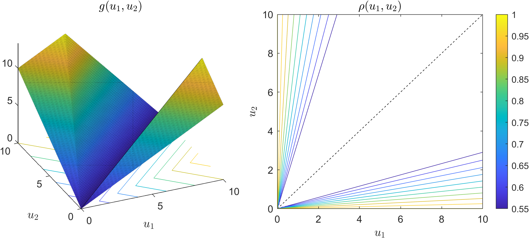
Figure 4: Example of the normalization function $g(u_{1},u_{2})=2\min\{|u_{1}-u_{2}|,(u_{1}+u_{2})/2\}$ and the relative convex inequity measure $\rho(u_{1},u_{2})=|u_{1}-u_{2}|/g(u_{1},u_{2})$.

Appendix D Solution Approaches with Convex Inequity Measures in Constraint Form

In this section, we propose solution approaches for optimization problem of the form (3) with our proposed convex inequity measures.

D.1 Absolute Convex Inequity Measure

Using the dual representation of absolute convex inequity measures (see Section 5), we can reformulate (3) into

$$\min_{\bm{x},\,\bm{u}}\Big{\{}f(\bm{u})\,\Big{|}\,\nu_{\bm{w}}(\bm{u})\leq\eta,\,\forall\bm{w}\in\mathcal{W}_{\nu},\,\bm{u}=U(\bm{x}),\,\bm{x}\in\mathcal{X}\Big{\}}.$$ (33)

Note that decision-makers typically specify the upper bound $\eta$ on the absolute convex inequity measure in (33). If they chose a very small $\eta$, then (33) could be infeasible.

Let us first consider the case when $\nu$ is an order-based inequity measure, i.e., $\mathcal{W}_{\nu}=\{\bm{w}\}$ is a singleton. Using the same proof techniques of Theorem 8, we can reformulate (33) as

$$\underset{\bm{x},\,\bm{u},\,\bm{\lambda}\in\mathbb{R}^{N},\,\bm{\theta}\in\mathbb{R}^{N}}{\textup{minimize}\,}\quad f(\bm{u})$$ (34a)

subject to $$\bm{1}^{\top}(\bm{\lambda}+\bm{\theta})\leq\eta,$$ (34b)

$$\lambda_{i}+\theta_{i^{\prime}}\geq u_{i}w_{i^{\prime}},\quad\forall i\in[N],\,i^{\prime}\in[N],$$ (34c)

$$\bm{u}=U(\bm{x}),\,\bm{x}\in\mathcal{X}.$$ (34d)

Second, when $\nu$ is an absolute convex inequity measure, we propose a C&CG algorithm similar to Algorithm 1 to solve (33). Algorithm 2 summarizes the steps of this algorithm. In this C&CG, we solve a master problem and a subproblem at each iteration. Specifically, at iteration $j$, we solve the following master problem:

$$\min_{\bm{x},\,\bm{u}}\Big{\{}f(\bm{u})\,\Big{|}\,\nu_{\bm{w}}(\bm{u})\leq\eta,\,\forall\bm{w}\in\{\bm{w}^{0},\dots,\bm{w}^{j-1}\},\,\bm{u}=U(\bm{x}),\,\bm{x}\in\mathcal{X}\Big{\}},$$ (35)

where $\{\bm{w}^{0},\dots,\bm{w}^{j-1}\}\subseteq\mathcal{W}_{\nu}$. Following the same techniques in the proof Proposition 6, we derive the following equivalent solvable reformulation of (35):

$$\underset{\bm{x},\,\bm{u},\,\bm{\lambda}\in\mathbb{R}^{N},\,\bm{\theta}\in\mathbb{R}^{N}}{\textup{minimize}\,}\quad f(\bm{u})$$ (36a)

subject to $$\bm{1}^{\top}(\bm{\lambda}^{k}+\bm{\theta}^{k})\leq\eta,\quad\forall k\in[0,j-1]_{\mathbb{Z}},$$ (36b)

$$\lambda^{k}_{i}+\theta^{k}_{i^{\prime}}\geq u_{i}w^{k}_{i^{\prime}},\quad\forall i\in[N],\,i^{\prime}\in[N],\,k\in[0,j-1]_{\mathbb{Z}},$$ (36c)

$$\bm{u}=U(\bm{x}),\,\bm{x}\in\mathcal{X}.$$ (36d)

Since only a set of weight vectors in $\mathcal{W}_{\nu}$ is considered, the master problem (36) is a relaxation of the original problem (33), i.e., the feasible region of (33) is a subset of the feasible region of (36). Thus, if (36) is infeasible, then we can conclude that the original problem (33) is also infeasible. Otherwise, with the optimal solution $\bm{u}^{j}$ from the master problem, we solve the same subproblem (16) and record the optimal solution $\bm{w}^{j}\in\mathcal{W}_{\nu}$ and optimal value $D^{j}$. Note that $D^{j}=\nu(\bm{u}^{j})$ is the value of the absolute inequity measure evaluated at $\bm{u}^{j}$. Thus, if $D^{j}>\eta$, the current solution $(\bm{x}^{j},\bm{u}^{j})$ is infeasible to the original problem (33), and thus we enlarge the set of weight vectors and proceed to the next iteration. Otherwise, we terminate and conclude that $(\bm{x}^{j},\bm{u}^{j})$ is an optimal solution.

Initialization : Set $LB=0$, $UB=\infty$, $\varepsilon>0$, $j=1$, $\bm{w}^{0}\in\mathcal{W}_{\nu}$.

1. Master problem.

     Solve master problem (36) with weights $\{\bm{w}^{0},\dots,\bm{w}^{j-1}\}$.

     If the master problem (36) is infeasible, terminate and return the infeasibility of (33).

     Otherwise, record the optimal solution $(\bm{x}^{j},\bm{u}^{j})$.

2. Subproblem. Solve subproblem (16) for fixed $\bm{u}=\bm{u}^{j}$.

     Record the optimal solution $\bm{w}^{j}$ and value $D^{j}$.

     If $D^{j}\leq\eta$, terminate and return the optimal solution $(\bm{x}^{j},\bm{u}^{j})$.

3. Scenario set enlargement.

     Update $j\leftarrow j+1$ and go back to step 1.

Algorithm 2 A column-and-constraint generation (C&CG) method to solve (33)

D.2 Relative Convex Inequity Measure

Recall that, in Section 5.2, we define a relative convex inequity measure by $\rho(\bm{u})=\nu(\bm{u})/g(\bm{u})$ for some absolute convex inequity measure $\nu$ and continuous normalization function $g$. Thus, the corresponding equity-promoting optimization model is

$$\min_{\bm{x},\,\bm{u}}\Big{\{}f(\bm{u})\,\Big{|}\,\rho(\bm{u})=\nu_{\bm{w}}(\bm{u})/g(\bm{u})\leq\eta,\,\forall\bm{w}\in\mathcal{W}_{\nu},\,\bm{u}=U(\bm{x}),\,\bm{x}\in\mathcal{X}\Big{\}}.$$ (37)

for some $\eta>0$. From Theorem 5, the normalization function $g$ satisfies $g\geq\nu\geq 0$. In particular, if $g(\bm{u})=0$, we must have $\nu(\bm{u})=0$. Therefore, we can reformulate (37) into

$$\min_{\bm{x},\,\bm{u}}\Big{\{}f(\bm{u})\,\Big{|}\,\nu_{\bm{w}}(\bm{u})\leq\eta g(\bm{u}),\,\forall\bm{w}\in\mathcal{W}_{\nu},\,\bm{u}=U(\bm{x}),\,\bm{x}\in\mathcal{X}\Big{\}},$$ (38)

which takes the same form of (33). Thus, we can apply similar solution approaches as in D.1 to solve (38).

Appendix E Implementation Details of Example 6.1

To generate the instances, for a given $|I|$, we randomly select $|I|$ different locations in the “2010 County Sorted 250” data from Daskin (2013), where we set $I=J$ as these locations. We compute the transportation cost using the Euclidean distance based on the locations’ latitude and longitude, and we set the demand as the location’s population. We implement the two reformulations in AMPL modeling language and use CPLEX (version 20.1.0.0) as the solver with default settings. We conduct all the experiments on a computer with an Intel Xeon Silver processor with a 2.10 GHz CPU and 128 Gb memory.

References

- Abul Naga and Yalcin (2008) Abul Naga, R.H., Yalcin, T., 2008. Inequality measurement for ordered response health data. Journal of Health Economics 27, 1614–1625.
- Ahmadi-Javid et al. (2017) Ahmadi-Javid, A., Seyedi, P., Syam, S.S., 2017. A survey of healthcare facility location. Computers & Operations Research 79, 223–263.
- Andreoli and Zoli (2020) Andreoli, F., Zoli, C., 2020. From unidimensional to multidimensional inequality: A review. Metron 78, 5–42.
- Armbruster and Delage (2015) Armbruster, B., Delage, E., 2015. Decision making under uncertainty when preference information is incomplete. Management Science 61, 111–128.
- Atkinson (1975) Atkinson, A.B., 1975. Economics of Inequality. Clarendon Press.
- Barbati and Piccolo (2016) Barbati, M., Piccolo, C., 2016. Equality measures properties for location problems. Optimization Letters 10, 903–920.
- Bateni et al. (2022) Bateni, M., Chen, Y., Ciocan, D.F., Mirrokni, V., 2022. Fair resource allocation in a volatile marketplace. Operations Research 70, 288–308.
- Bertsekas (2009) Bertsekas, D., 2009. Convex Optimization Theory. Athena Scientific.
- Bertsekas (2015) Bertsekas, D., 2015. Convex Optimization Algorithms. Athena Scientific.
- Bertsimas et al. (2013) Bertsimas, D., Farias, V.F., Trichakis, N., 2013. Fairness, efficiency, and flexibility in organ allocation for kidney transplantation. Operations Research 61, 73–87.
- Bertsimas and Shtern (2018) Bertsimas, D., Shtern, S., 2018. A scalable algorithm for two-stage adaptive linear optimization. arXiv preprint arXiv:1807.02812 .
- Blanco et al. (2016) Blanco, V., Puerto, J., Ben-Ali, S.E.H., 2016. Continuous multifacility ordered median location problems. European Journal of Operational Research 250, 56–64.
- Breugem et al. (2022) Breugem, T., Dollevoet, T., Huisman, D., 2022. Is equality always desirable? Analyzing the trade-off between fairness and attractiveness in crew rostering. Management Science 68, 2619–2641.
- Castillo and Ruiz-Cobo (1992) Castillo, E., Ruiz-Cobo, M.R., 1992. Functional Equations and Modelling in Science and Engineering. volume 161. CRC Press.
- Celik Turkoglu and Erol Genevois (2020) Celik Turkoglu, D., Erol Genevois, M., 2020. A comparative survey of service facility location problems. Annals of Operations Research 292, 399–468.
- Chakravarty (1999) Chakravarty, S.R., 1999. Measuring inequality: The axiomatic approach. Handbook of Income Inequality Measurement , 163–186.
- Chakravarty (2007) Chakravarty, S.R., 2007. A deprivation-based axiomatic characterization of the absolute Bonferroni index of inequality. The Journal of Economic Inequality 5, 339–351.
- Chang et al. (2018) Chang, D., Lin, M., Zhang, C., 2018. On the generalization ability of online gradient descent algorithm under the quadratic growth condition. IEEE Transactions on Neural Networks and Learning Systems 29, 5008–5019.
- Chen and Hooker (2023) Chen, V.X., Hooker, J., 2023. A guide to formulating fairness in an optimization model. Annals of Operations Research , 1–39.
- Cowell (2011) Cowell, F., 2011. Measuring Inequality. Oxford University Press.
- Cowell (2000) Cowell, F.A., 2000. Measurement of inequality. Handbook of Income Distribution 1, 87–166.
- Cowell and Kuga (1981) Cowell, F.A., Kuga, K., 1981. Inequality measurement: An axiomatic approach. European Economic Review 15, 287–305.
- Csiszar (2021) Csiszar, O., 2021. Ordered weighted averaging operators: A short review. IEEE Systems, Man, and Cybernetics Magazine 7, 4–12.
- Dalton (1920) Dalton, H., 1920. The measurement of the inequality of incomes. The Economic Journal 30, 348–361.
- Daskin (2013) Daskin, M.S., 2013. Network and Discrete Location: Models, Algorithms, and Applications, Second Edition. John Wiley & Sons, Ltd.
- Diakonikolas et al. (2020) Diakonikolas, J., Fazel, M., Orecchia, L., 2020. Fair packing and covering on a relative scale. SIAM Journal on Optimization 30, 3284–3314.
- Donaldson and Weymark (1980) Donaldson, D., Weymark, J.A., 1980. A single-parameter generalization of the Gini indices of inequality. Journal of Economic Theory 22, 67–86.
- Dönmez et al. (2022) Dönmez, Z., Ayyıldız, M., Uslu, B., Karsu, O., Y Kara, B., 2022. Fairness in humanitarian logistics: State of the art and future directions. Available at SSRN: https://ssrn.com/abstract=4396254 .
- Filippi et al. (2021) Filippi, C., Guastaroba, G., Speranza, M.G., 2021. On single-source capacitated facility location with cost and fairness objectives. European Journal of Operational Research 289, 959–974.
- Foster (1983) Foster, J.E., 1983. An axiomatic characterization of the theil measure of income inequality. Journal of Economic Theory 31, 105–121.
- Gini (1912) Gini, C., 1912. Variabilità e Mutabilità: Contributo allo Studio delle Distribuzioni e delle Relazioni Statistiche. Cuppini, Bologna.
- Gutjahr and Fischer (2018) Gutjahr, W.J., Fischer, S., 2018. Equity and deprivation costs in humanitarian logistics. European Journal of Operational Research 270, 185–197.
- Hooker and Williams (2012) Hooker, J.N., Williams, H.P., 2012. Combining equity and utilitarianism in a mathematical programming model. Management Science 58, 1682–1693.
- Hoover (1936) Hoover, E.M., 1936. The measurement of industrial localization. The Review of Economic Statistics , 162–171.
- Hu et al. (2018) Hu, J., Bansal, M., Mehrotra, S., 2018. Robust decision making using a general utility set. European Journal of Operational Research 269, 699–714.
- Jagtenberg and Mason (2020) Jagtenberg, C.J., Mason, A.J., 2020. Improving fairness in ambulance planning by time sharing. European Journal of Operational Research 280, 1095–1107.
- Jancewicz (2016) Jancewicz, B., 2016. Income inequalities: Axioms of income inequality measures and people’s perceptions. Decyzje .
- Kakwani (1980) Kakwani, N., 1980. On a class of poverty measures. Econometrica: Journal of the Econometric Society , 437–446.
- Karsu and Morton (2015) Karsu, Ö., Morton, A., 2015. Inequity averse optimization in operational research. European Journal of Operational Research 245, 343–359.
- Kolm (1976) Kolm, S.C., 1976. Unequal inequalities. I. Journal of Economic Theory 12, 416–442.
- Kostreva et al. (2004) Kostreva, M.M., Ogryczak, W., Wierzbicki, A., 2004. Equitable aggregations and multiple criteria analysis. European Journal of Operational Research 158, 362–377.
- Lan et al. (2010) Lan, T., Kao, D., Chiang, M., Sabharwal, A., 2010. An axiomatic theory of fairness in network resource allocation, in: 2010 Proceedings IEEE INFOCOM, pp. 1–9. doi:10.1109/INFCOM.2010.5461911.
- Lejeune and Turner (2019) Lejeune, M.A., Turner, J., 2019. Planning online advertising using Gini indices. Operations Research 67, 1222–1245.
- Lewis et al. (2021) Lewis, E.O., MacKenzie, D., Kaminsky, J., 2021. Exploring equity: How equity norms have been applied implicitly and explicitly in transportation research and practice. Transportation Research Interdisciplinary Perspectives 9, 100332.
- Li et al. (2022) Li, H., Delage, E., Zhu, N., Pinedoc, M., Ma, S., 2022. Distributional robustness and inequity mitigation in disaster preparedness of humanitarian operations. Optimization Online .
- Liu et al. (2019) Liu, Y., Pichler, A., Xu, H., 2019. Discrete approximation and quantification in distributionally robust optimization. Mathematics of Operations Research 44, 19–37.
- Marsh and Schilling (1994) Marsh, M.T., Schilling, D.A., 1994. Equity measurement in facility location analysis: A review and framework. European Journal of Operational Research 74, 1–17.
- Marshall et al. (2011) Marshall, A.W., Olkin, I., Arnold, B.C., 2011. Inequalities: Theory of Majorization and its Applications. Springer.
- Martello and Toth (1987) Martello, S., Toth, P., 1987. Linear assignment problems, in: North-Holland Mathematics Studies. Elsevier. volume 132, pp. 259–282.
- Marynissen and Demeulemeester (2019) Marynissen, J., Demeulemeester, E., 2019. Literature review on multi-appointment scheduling problems in hospitals. European Journal of Operational Research 272, 407–419.
- Mehran (1976) Mehran, F., 1976. Linear measures of income inequality. Econometrica: Journal of the Econometric Society , 805–809.
- Mesa et al. (2003) Mesa, J.A., Puerto, J., Tamir, A., 2003. Improved algorithms for several network location problems with equality measures. Discrete Applied Mathematics 130, 437–448.
- Mo and Walrand (2000) Mo, J., Walrand, J., 2000. Fair end-to-end window-based congestion control. IEEE/ACM Transactions on Networking 8, 556–567.
- Mostajabdaveh et al. (2019) Mostajabdaveh, M., Gutjahr, W.J., Sibel Salman, F., 2019. Inequity-averse shelter location for disaster preparedness. IISE Transactions 51, 809–829.
- Moulin (2004) Moulin, H., 2004. Fair Division and Collective Welfare. MIT Press.
- Mussard and Mornet (2019) Mussard, S., Mornet, P., 2019. A note on -Gini measures. Review of Income and Wealth 65, 675–682.
- Nickel and Puerto (2006) Nickel, S., Puerto, J., 2006. Location Theory: A Unified Approach. Springer Science & Business Media.
- Ogryczak (2000) Ogryczak, W., 2000. Inequality measures and equitable approaches to location problems. European Journal of Operational Research 122, 374–391.
- Ogryczak and Śliwiński (2006) Ogryczak, W., Śliwiński, T., 2006. On direct methods for lexicographic min-max optimization, in: International Conference on Computational Science and Its Applications, Springer. pp. 802–811.
- Pichler and Xu (2018) Pichler, A., Xu, H., 2018. Quantitative stability analysis for minimax distributionally robust risk optimization. Mathematical Programming , 1–31.
- Pinedo (2016) Pinedo, M.L., 2016. Scheduling: Theory, Algorithms, and Systems. Springer.
- Rahmattalabi et al. (2022) Rahmattalabi, A., Vayanos, P., Dullerud, K., Rice, E., 2022. Learning resource allocation policies from observational data with an application to homeless services delivery, in: 2022 ACM Conference on Fairness, Accountability, and Transparency, pp. 1240–1256.
- Rawls (1999) Rawls, J., 1999. A Theory of Justice: Revised Edition. Harvard University Press.
- Rockafellar (1970) Rockafellar, R.T., 1970. Convex Analysis. volume 18. Princeton University Press.
- Rodríguez-Chía et al. (2000) Rodríguez-Chía, A.M., Nickel, S., Puerto, J., Fernandez, F.R., 2000. A flexible approach to location problems. Mathematical Methods of Operations Research 51, 69–89.
- Shapiro (1994) Shapiro, A., 1994. Quantitative stability in stochastic programming. Mathematical Programming 67, 99–108.
- Shehadeh and Snyder (2021) Shehadeh, K.S., Snyder, L.V., 2021. Equity in stochastic healthcare facility location. arXiv preprint arXiv:2112.03760 .
- Shen et al. (2019) Shen, S., Qian, J., Cheng, D., Yang, K., Zhang, G., 2019. A sum-utility maximization approach for fairness resource allocation in wireless powered body area networks. IEEE Access 7, 20014–20022.
- Stancu-Minasian (1997) Stancu-Minasian, I.M., 1997. Fractional Programming: Theory, Methods and Applications. volume 409. Springer Dordrecht.
- Stȩpniak (2007) Stȩpniak, C., 2007. An effective characterization of Schur-convex functions with applications. Journal of Convex Analysis 14, 103–108.
- Sun et al. (2023) Sun, L., Wei, P., Xie, W., 2023. Fair and risk-averse urban air mobility resource allocation under uncertainties. Available at SSRN 4343979 .
- Sun et al. (2022) Sun, L., Xie, W., Witten, T., 2022. Distributionally robust fair transit resource allocation during a pandemic. Transportation Science .
- Theil (1967) Theil, H., 1967. Economics and Information Theory. North-Holland.
- Thon (1982) Thon, D., 1982. An axiomatization of the gini coefficient. Mathematical Social Sciences 2, 131–143.
- Uhde et al. (2020) Uhde, A., Schlicker, N., Wallach, D.P., Hassenzahl, M., 2020. Fairness and decision-making in collaborative shift scheduling systems, in: Proceedings of the 2020 CHI Conference on Human Factors in Computing Systems, pp. 1–13.
- Williams and Cookson (2000) Williams, A., Cookson, R., 2000. Equity in health. Handbook of Health Economics 1, 1863–1910.
- Williamson and Menon (2019) Williamson, R., Menon, A., 2019. Fairness risk measures, in: International Conference on Machine Learning, PMLR. pp. 6786–6797.
- Yager (1988) Yager, R.R., 1988. On ordered weighted averaging aggregation operators in multicriteria decisionmaking. IEEE Transactions on Systems, Man, and Cybernetics 18, 183–190.
- Zhang et al. (2021) Zhang, J., Liu, Y., Yu, G., Shen, Z.J., 2021. Robustifying humanitarian relief systems against travel time uncertainty. Naval Research Logistics 68, 871–885.
- Zheng (2007) Zheng, B., 2007. Unit-consistent decomposable inequality measures. Economica 74, 97–111.