Improving the predictions of ML-corrected climate models with novelty detection

Abstract

While previous works have shown that machine learning (ML) can improve the prediction accuracy of coarse-grid climate models, these ML-augmented methods are more vulnerable to irregular inputs than the traditional physics-based models they rely on. Because ML-predicted corrections feed back into the climate model’s base physics, the ML-corrected model regularly produces out of sample data, which can cause model instability and frequent crashes. This work shows that adding semi-supervised novelty detection to identify out-of-sample data and disable the ML-correction accordingly stabilizes simulations and sharply improves the quality of predictions. We design an augmented climate model with a one-class support vector machine (OCSVM) novelty detector that provides better temperature and precipitation forecasts in a year-long simulation than either a baseline (no-ML) or a standard ML-corrected run. By improving the accuracy of coarse-grid climate models, this work helps make accurate climate models accessible to researchers without massive computational resources.

1 Introduction

Accurate climate models are essential for diagnosing the general trends of climate change and predicting its localized impacts. Given finite resources, having computationally efficient models is also important to assess climate policies by making simulations cheap and easy. Previous works [1, 2, 3, 4, 5] have suggested that augmenting physics-based climate models with machine learning can reduce bias and improve the overall skill of coarse climate models, while sometimes introducing instability. This work draws on the idea of using a compound parameterization [6, 7] to mask ML models with high uncertainty and builds on those ML-corrected models by incorporating out-of-sample detection. Our approach adds stability and outperforms these past approaches (specifically, [3, 8]) on temperature and precipitation metrics.

We model the atmosphere as a system of partial differential equations (PDEs). The atmospheric state is modeled as $X=(x_{1},\dots,x_{N})\in\mathbb{R}^{d\times N}$, a three-dimensional grid of $N$ latitude/longitude coordinates with $d$-dimensional column vectors of air temperature, specific humidity, and other fields. The state of a particular column $x_{i}\in\mathbb{R}^{d}$ evolves over time as

$$\frac{dx_{i}}{dt}=f_{i}(X,t)$$ (1)

for some fixed $f_{i}$ derived from physically-based assumptions; we refer to this as the baseline model. The size of $N$ corresponds to the grid resolution; large $N$ yields more accurate but computationally expensive simulations.

While accuracy penalties due to a loss of resolution are expected for small $N$, coarse-grid simulations are additionally biased by poor representations of subgrid-scale processes like thunderstorms and cloud radiative effects [9, 10]. ML is an appealing way to de-bias this coarse climate model by predicting and compensating for its error. Put precisely, the ML-corrected model is

$$\frac{dx_{i}}{dt}=f_{i}(X,t)+g(x_{i},q_{i};\theta),$$ (2)

where $g(\cdot;\theta):\mathbb{R}^{d+3}\to\mathbb{R}^{d}$ is a learned function with parameters $\theta$ that predicts corrective tendencies from the column, $x_{i}\in\mathbb{R}^{d}$, and its insolation, surface elevation, and latitude $q_{i}\in\mathbb{R}^{3}$. The ML correction enables the baseline to better approximate a reference fine-grid model while maintaining the underlying physics as the core of the modeling approach [2, 3].

While ML-based models frequently improve overall error, these models—especially deep neural networks—are often not robust, meaning they perform poorly with out-of-sample data that lies outside the training distribution. In online application (where predictions are fed back into the model repeatedly for a simulation) of these models, ML model errors accumulate in time and overwhelm the damping mechanisms of the baseline physics [11]. In past works [8], letting $x_{i}$ represent a vertical column of air temperature and specific humidity values resulted in an accurate and stable model, but including horizontal winds in $x_{i}$ caused the model to crash or be more inaccurate for certain fields within a few simulated weeks. Other works [12] have stabilized ML-corrected climate models by tapering upper-atmospheric outputs to zero and removing upper-atmospheric inputs when learning $g$, but this approach has not been applied to models with wind tendencies.

This poses a dilemma: By omitting the wind tendencies from $g$, the model is unable to incorporate relevant climate information into its predictions. Yet including the wind tendencies introduces new instabilities. We fix this by employing semi-supervised novelty detection to predict when a column $x_{i}$ belongs to the training distribution of $g$ and suppress the tendencies of the ML model if not. Our model has the form

$$\frac{dx_{i}}{dt}=f_{i}(X,t)+\eta(x_{i};\rho)g(x_{i},q_{i};\theta),$$ (3)

for a novelty detector $\eta(\cdot;\rho):\mathbb{R}^{d}\to[0,1]$. A properly tuned $\eta$ improves coarse climate model temperature and precipitation forecasts for at least a year.

2 Methodology

2.1 ML-corrected climate models and data

We consider two neural networks for modeling the ML-corrected tendencies. $g_{\mathrm{Tq}}$ corrects vertical columns with 79 pressure levels containing only air temperatures (T) and specific humidities (q); thus, $d=2\cdot 79$. $g_{\mathrm{Tquv}}$ additionally corrects eastward and northward wind velocities (u, v); $d=4\cdot 79$. We train the these corrective functions to predict an observed “nudging” vector between a pre-existing fine-grid simulation (with much larger $N$) and a simulated coarse-grid run [3, 8]. We use a dataset $\{x^{(t)}_{i}\in\mathbb{R}^{d}:t\in[T],i\in[N]\}$ with $T$ time steps generated by the same simulation as the training set to train the novelty detector $\eta(\cdot,\rho)$. These models are described in greater depth in Appendix A.

2.2 Novelty detection

The novelty detector $\eta$ predicts whether a column $x$ belongs within the support of the training set. If so, then we let $\eta(x;\rho)=1$ to take full advantage of the learned correction $g(x,q;\theta)$; otherwise, we ignore $g(\cdot;\theta)$ by setting $\eta(x;\rho)=0$.

Novelty detection is a well-studied semi-supervised learning problem about estimating the support of a dataset using only positive examples [13]. We frame the problem as novelty detection rather than outlier detection (an unsupervised problem with mixture of in-distribution and out-of-distribution samples) or standard two-class supervised classification because we have no dataset of representative out-of-distribution samples. There are many known approaches to novelty detection, including local-outlier factor [14], $k$-means clustering [15], and minimum-volume ellipsoid estimation [16]. Our exploratory work considers two of these approaches: a simple “min-max” novelty detector and a one-class support vector machine (OCSVM). For each of these we consider novelty detectors $\eta_{\mathrm{T}}$ with 79-dimensional temperature vectors as input and $\eta_{\mathrm{Tq}}$ with 158-dimensional combined temperature and specific humidity vectors.

Naive “min-max” novelty detector

The min-max novelty detector considers the smallest axis-aligned hyper-rectangle that contains all training samples and categorizes any sample outside the rectangle as a novelty. Put concretely,

$$\eta_{\mathrm{minmax}}(x;(x_{\min},x_{\max}))=\begin{cases}1&\text{if }x_{k}\in[x_{\min,k},x_{\max,k}]\ \forall k\in[d],\\ 0&\text{otherwise,}\end{cases}$$

for $x_{\min,k}=\min_{i,t}x^{(t)}_{i,k}$ and $x_{\max,k}=\max_{i,t}x^{(t)}_{i,k}$ as the minimum and maximum over the training data of the $k$th feature. While efficient, this novelty detector is unable to identify irregularities within the bounding box.

One-class support vector machine (OCSVM)

The one-class SVM algorithm of [17] repurposes the SVM classification algorithm to estimate the support of a distribution by finding the maximum-margin hyperplane separating training samples from the origin. The OCSVM has been applied to novelty detection for genomics [18], video footage [19], propulsion systems [20], and the internet of things [21]. We normalize each input $x_{i}$ and lift it to the infinite-dimensional feature space $\phi(x_{i})$ corresponding to the radial basis function (RBF) kernel $\kappa_{\gamma}(x,x^{\prime})=\exp(-\gamma\|x-x^{\prime}\|_{2}^{2})$. We use the novelty detector

$$\eta_{\mathrm{OCSVM}}(x;(\alpha,\nu,\gamma))=\begin{cases}1&\text{if }\sum_{t=1}^{T}\sum_{i=1}^{N}\alpha_{t,i}\kappa_{\gamma}(x,x_{i}^{(t)})\geq\nu,\\ 0&\text{otherwise,}\end{cases}$$

whose weights $\alpha_{i}\geq 0$ are determined by a quadratic program based on the training data and whose sensitivity is set by cutoff $\nu>0$. The prediction rule depends exclusively on the number of support vectors, or training samples $x_{i}^{(t)}$ with $\alpha_{t,i}>0$. To obtain a robust and computationally efficient novelty detector, we restrict the model at have most a $10^{-4}$ fraction of samples as support vectors. Smaller values of $\gamma$ correspond to novelty detectors that with highly smoothed support estimations that may be larger than necessary, while large $\gamma$ provides a smaller and higher variance region. Our experiments train and evaluate numerous novelty detectors for several choices of $\gamma$ and $\nu$.

3 Results

Because there is no ground-truth verdict about whether a data point is out-of-distribution, we evaluate our novelty detectors by incorporating $\eta(\cdot;\rho)$ into the coarse grid model, numerically simulating equation (3) for one year at 15-minute time increments at C48 resolution, and comparing the predicted atmospheric states $\hat{x}_{i}^{(t)}$ to $x_{\mathrm{fine},i}^{(t)}$ using the root mean square error (RMSE) of three time-averaged diagnostics (see equation (5)): near-surface air temperatures at 850hPa of pressure (T), surface precipitation rate (SP), and precipitable water (PWAT). Table 1 compares the performances of seven global simulations. The first is the baseline simulation of equation (1); the next two are ML-corrected runs from equation (2) without and with wind tendency corrections; and the remaining four simulations include novelty detection from equation (3) and differ in the choice of novelty detector and the inputs to $g$ and $\eta$. The OCSVMs use RBF parameter $\gamma=\frac{4}{79}$ and cutoff

$$\nu=\min_{i^{\prime},t^{\prime}}\sum_{t}\sum_{i}\alpha_{t,i}\kappa_{\gamma}(x_{i^{\prime}}^{(t^{\prime})},x_{i}^{(t)})$$ (4)

set to be the smallest OCSVM score observed in the training set.

Table 1: The RMSE scores of time-averaged metrics and novelty detection rates for year-long runs. The third run crashed after 38 days (denoted with a star), so its metrics are averaged over 38-days rather than one year. The “% Novelty” column represents the fraction of columns of the simulated run without ML-corrections. Metrics are 850-hPa temperature (T), surface precipitation rate (SP) and precipitable water (PWAT).

	Run	% Novelty	T ($\mathrm{K}$)	SP ($\mathrm{mm}/\mathrm{day}$)	PWAT ($\mathrm{kg}/\mathrm{m}^{2}$)
1	Baseline (1)	100%	2.09	1.78	2.79
2	ML-corrected (2) with $g_{\mathrm{Tq}}$	0%	1.86	1.43	3.31
3	ML-corrected with $g_{\mathrm{Tquv}}$ ($\star$)	0%	2.43	3.39	5.33
4	ND ML (3) with $g_{\mathrm{Tq}},\eta_{\mathrm{T,OCSVM}}$	2.5%	1.97	1.49	3.65
5	ND ML with $g_{\mathrm{Tquv}},\eta_{\mathrm{T,minmax}}$	35.7%	5.15	3.57	10.14
6	ND ML with $g_{\mathrm{Tquv}},\eta_{\mathrm{T,OCSVM}}$	40.0%	1.58	1.40	2.66
7	ND ML with $g_{\mathrm{Tquv}},\eta_{\mathrm{Tq,OCSVM}}$	50.7%	1.53	1.24	2.37

The baseline model (1) outperforms the ML-corrected model with winds without novelty detection (3). In particular, the simulation of (3) crashed after 38 days due to model instability. Applying novelty detection in (4) to (2) preserves the stability of the model without across-the-board improvements. The min-max novelty detector (5) avoids the crash of (3), but otherwise performs far worse than other approaches, indicating the importance of representing the data distribution with a more meaningful quantity than a bounding box. Both OCSVM novelty detection models with $g_{\mathrm{Tquv}}$ (6, 7) dominate all other models on all metrics, and the final model with $\eta_{\mathrm{Tq}}$ (7) performs best on all metrics. These results suggest that suppressing ML corrections to atypical temperature or specific humidity columns is sufficient to realize the advantages of incorporating horizontal winds into the ML-corrected model, which ML-only models fail to achieve. These models find a “sweet spot” between the ML-corrected and baseline approaches and stabilizes the ML corrections, reducing model bias without suffering from catastrophic behavior caused by out-of-sample errors, as illustrated for temperature in Figure 1.

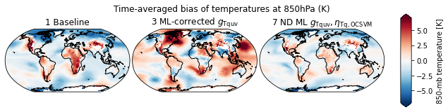
Figure 1: The OCSVM model (7, right) moderates the extreme behavior w.r.t. near-surface temperatures of both the baseline model (1, left) and the crashed ML-corrected run (3, center).

As visualized by Figure 2, the number of novelties in each run with wind included in the ML corrections quickly spikes to include 40 to 70% of the grid points (weighted by corresponding land area). The most successful approaches are thus highly aggressive, identifying a wide range of columns as novelties and removing them from consideration to erratic behavior. While the novelty detection models flag a large fraction of columns, this behavior remains relatively stable over time, which indicates that these climate models are unlikely to converge to an “effectively baseline” solution, in which all columns are classified as novelties and ML corrections are never incorporated.

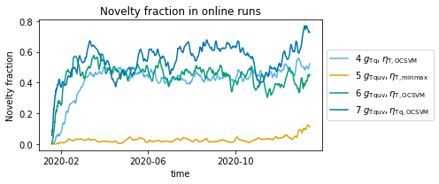
Figure 2: Percentage of novelties weighted by grid cell size for year-long runs (4-7).

We walk through an explicit example of how these novelty detectors preempt model instability in Appendix C. Appendix D shows that varying $\nu$ interpolates between the always-novelty (baseline) and never-novelty (ML-corrected) regimes for a variety of $\gamma$ choices and has optimal model performance between those extremes.

4 Conclusion and future work

Applying novelty detection to coarse ML-corrected atmospheric climate models improves the quality of temperature and precipitation estimates of coarse climate models by permitting the introduction of wind tendencies to the corrective model without instabilities. Future work can build on this by experimenting with different novelty detection approaches, OCSVM kernels, inputs to $g$ and $\eta$, and methods of integration with the ML-corrected climate model.

Appendix A Training details for ML-correction $g$

A.1 Dataset

We train the corrective tendencies offline as described by [3, 8]. That is, $g(\cdot;\theta)$ is trained on samples $((x^{(t)}_{i},q_{i}),y_{i}^{(t)})$ to ensure $g(x^{(t)}_{i},q_{i};\theta)\approx y^{(t)}_{i}$ for nudging tendency labels $y^{(t)}_{i}$ to be defined. We obtain the samples by combining the results of two simulations of baseline climate models with $T$ time steps and $N$ grid cells:

• $X^{(1)},\dots,X^{(T)}\in\mathbb{R}^{N\times d}$ are a sequence of observed time steps of the nudged coarse run with $N$ grid cells described in [3] that that are corrected at each step with the observed nudging tencies $Y^{(1)},\dots,Y^{(T)}$. We use a version of FV3GFS [24] with a C48 cubed-sphere grid of approximately 200 km horizontal resolution [25] for our coarse-grid model $f_{i}$. In this grid, the Earth is divided into 6 square tiles with a 48-by-48 grid imposed on each ($N=6\cdot 48^{2}$).

• $X_{\mathrm{fine}}^{(1)},\dots,X_{\mathrm{fine}}^{(T)}\in\mathbb{R}^{N\times d}$ are generated by a simulating a fine-grid model with $N_{\mathrm{fine}}\gg N$ grid cells with equation (1) and coarsening its output to have resolution $N$. The fine-grid reference model used by [26] to train the ML has a similar type of grid with a much finer resolution of 3 km.

We scale the difference between the coarse model and its highly accurate fine-grained counterpart in order to obtain $d$-dimensional nudging tendencies,

$$y^{(t)}_{i}:=\frac{x^{(t)}_{\mathrm{fine},i}-x_{i}^{(t)}}{\tau},$$

for nudging timescale $\tau$. Samples are collected by running a year-long coarse-grid simulation nudged to the fine-grid model state with a 3 hour nudging timescale; the state and nudging tendencies are saved every 3 hours. After dividing this data into interleaved time blocks for the train/test split and subsampling down to 15% of the columns in each timestep, we are left with $n=2834611$ training samples.

The same dataset $\{x^{(t)}_{i}\in\mathbb{R}^{d}:t\in[T],i\in[N]\}$ is used to train the novelty detector $\eta(\cdot;\rho)$. The nudges $y_{i}^{(t)}$ are omitted, as the novelty detection procedure requires no labels.

A.2 ML-corrected climate models

We consider two nudging tendency models: $g_{\mathrm{Tq}}$ and $g_{\mathrm{Tquv}}$.

• $g_{\mathrm{Tq}}$ is a no-wind model that corrects vertical columns of air temperature (T) and specific humidity (q). That is, $x_{i}$ is a $d=(2\cdot 79)$-dimensional vector with 79 temperature and 79 humidity coordinates, each corresponding to a pressure-level in the atmosphere.

• $g_{\mathrm{Tquv}}$ also corrects horizontal wind tendencies (u, v), which modify the two-dimensional wind velocity at each altitude, making $x_{i}$ a $d=(4\cdot 79)$-dimensional vector.

$g_{\mathrm{Tq}}(\cdot;\theta):\mathbb{R}^{158}\times\mathbb{R}^{3}\to\mathbb{R}^{158}$ predicts the temperature and humidity nudge vector $y_{i}^{(t)}$ from temperature and humidity state $x_{i}^{(t)}$, as well as the insolation, surface elevation, and latitude $q_{i}$ of the corresponding cell. We represent $g_{Tq}(\cdot;\theta)$ as a three-layer dense multi-layer perceptron of width 419. The loss is measured by the mean absolute error (MAE) with kernel regularization with parameter $10^{-4}$. We train the model with Adam for 500 epochs using a fixed learning rate of $0.00014$ and a batch size of 512 samples. For the sake of stability, the model sets to zero the learned nudges for the three highest altitude temperature and humidity values; that is, $g_{\mathrm{Tq}}(\cdot;\theta)$ can be properly thought of as a function of the form $\mathbb{R}^{158}\times\mathbb{R}^{3}\to\mathbb{R}^{152}$.

On the other hand, $g_{\mathrm{Tquv}}(\cdot;\theta):\mathbb{R}^{316}\times\mathbb{R}^{3}\to\mathbb{R}^{316}$ is defined as the concatenation of two learned functions for input $x=(x_{\mathrm{Tq}},x_{\mathrm{uv}})\in\mathbb{R}^{158}\times\mathbb{R}^{158}$:

$$g_{\mathrm{Tquv}}(x,q;\theta)=(g_{\mathrm{Tq}}(x_{\mathrm{Tq}},q;\theta_{\mathrm{Tq}}),g_{\mathrm{uw}}(x_{\mathrm{Tq}},x_{\mathrm{uw}},q;\theta_{\mathrm{uv}})).$$

$g_{\mathrm{Tq}}(\cdot;\theta_{\mathrm{Tq}})$ is trained identically to the aforementioned model. $g_{\mathrm{uv}}(\cdot;\theta_{\mathrm{uv}}):\mathbb{R}^{316}\times\mathbb{R}^{3}\to\mathbb{R}^{158}$ is separately trained to infer wind nudges from temperatures, humidities, and horizontal winds. Besides the different input dimension, $g_{\mathrm{uv}}(\cdot;\theta_{\mathrm{uv}})$ is otherwise structured and trained identically to the other model.

A.3 Computing scalar metrics

As mentioned in Section 3, we measure the success of a coarse-grid simulated run by computing the RMSE of time-averaged quantities (850hPa temperature, surface precipitation, total precipitable water) with respect to those same quantities of the fine grid run. We compute each with the following expression:

$$\sqrt{\sum_{i=1}^{N}a_{i}\left(\frac{1}{T}\sum_{t=1}^{T}\left(\hat{s}_{i}^{(t)}-s_{\mathrm{fine},i}^{(t)}\right)\right)^{2}},$$ (5)

letting $\hat{s}_{i}^{(t)}$ and $s_{\mathrm{fine},i}^{(t)}$ reflect the quantity at grid cell $i\in[N]$ and time $t\in[T]$ in our coarse-grid and the reference fine-grid simulations respectively and $a_{i}$ represent the normalized area weights of grid cells.

Appendix B Comparing continuous and threshold-based novelty detectors $\eta(\cdot;\rho)$

The results in Section 3 demonstrate the empirical success of the OCSVM novelty detector applied as a discrete on-off switch for the corrective tendencies in equation (3). However, this method creates sharp discontinuities in the nudging tendencies (see the left panel of Figure 3), since the tendencies are often at their most extreme when the respective temperature columns are nearly out of sample. As a potential remedy, we consider several approaches to smoothing these sharp novelty detection functions $\eta$ and ask whether they (1) subjectively smooth the tendencies to avoid such sharp thresholds and (2) result in better (at least, not worse) online model performance.

We represent the generalized OCSVM novelty detector applied to temperature columns as

$$\eta_{\mathrm{T,OCSVM}}(x;(\alpha,\nu,\gamma,\psi))=\psi\left(\sum_{t=1}^{T}\sum_{i=1}^{N}\alpha_{t,i}\kappa_{\gamma}(x,x_{i}^{(t)})-\nu\right),$$

for some link function $\psi:\mathbb{R}\to[0,1]$. We consider three choices for $\psi$.

1. $\psi_{\mathrm{mask}}$ is the sharp threshold function used in the paper body:

   $$\psi_{\mathrm{mask}}(z)=\begin{cases}1&\text{if }z\geq 0,\\ 0&\text{if }z<0.\end{cases}$$

2. $\psi_{\mathrm{ramp},\zeta}$ linearly interpolates between 1 at $\zeta>0$ and 0 at $-\zeta$:

   $$\psi_{\mathrm{ramp},\zeta}(z)=\begin{cases}1&\text{if }z\geq\zeta,\\ \frac{z+\zeta}{2\zeta}\ &\text{if }z\in[-\zeta,\zeta],\\ 0&\text{if }z\leq-\zeta.\end{cases}$$

3. $\psi_{\mathrm{decay},\zeta,\beta}$ exponentially decays at a rate of $\beta\in(0,1)$ starting at the threshold $\zeta$:

   $$\psi_{\mathrm{decay},\zeta,\beta}(z)=\begin{cases}1&\text{if }z\geq\zeta,\\ \beta^{\zeta-z}&\text{if }z\leq\zeta.\end{cases}$$

While numerous other sigmoidal functions can be considered, we restrict our focus to these three. We use the same ML correction $g_{\mathrm{Tquv}}$ and OCSVM model with trained $\alpha$ and $\gamma=\frac{4}{79}$ and compare the performances of several simulated runs of equation (3) with different link functions $\psi$.

Table 2 illustrates that the choice of link function $\psi$ has a marginal impact on the scalar quality metrics, with the ramp function besting the masked approach at temperature and precipitation accuracy while falling short on precipitable water. Figure 3 shows that these link functions have a locally smoothing effect on the magnitudes of the learned tendencies; both ramp and decay link functions avoid the sharp separations between complete suppression and expression of strong corrections from the masking link function.

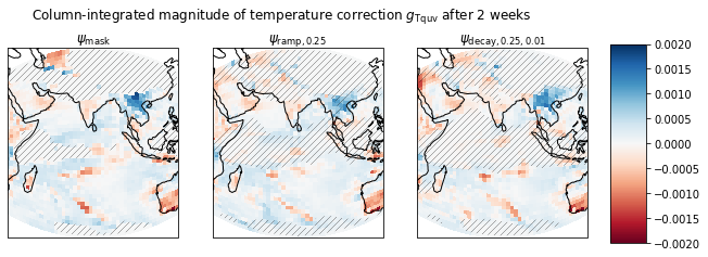
Figure 3: Integrated horizontal wind tendencies after novelty detection is applied at a fixed time-step $t$ after two weeks of simulation on a simulation of equation (3) with different choices of link function $\psi_{\mathrm{mask}}$ (left), $\psi_{\mathrm{ramp},0.25}$ (center), and $\psi_{\mathrm{decay},-0.25,0.01}$ (right) with $g_{\mathrm{Tquv}}$ and $\eta_{\mathrm{T,OCSVM}}$ with $\gamma=\frac{4}{d}$ trained on temperature tendencies. The hatched regions have some amount of ML-correction suppression (i.e. $\eta_{\mathrm{T,OCSVM}}(x;\rho)<1$).

Table 2: A comparison of RMSEs of time-averaged metrics over year-long simulations of equation (3) with different choices of link function $\psi$ with $g_{\mathrm{Tquv}}$ and $\eta_{\mathrm{T,ocsvm}}$ as discussed in Section 3.

	Run	T ($\mathrm{K}$)	SP ($\mathrm{mm}/\mathrm{day}$)	PWAT ($\mathrm{kg}/\mathrm{m}^{2}$)
1	$\psi_{\mathrm{mask}}$	1.58	1.40	2.66
2	$\psi_{\mathrm{ramp},0.1}$	1.49	1.36	2.73
3	$\psi_{\mathrm{ramp},0.25}$	1.53	1.36	2.71
4	$\psi_{\mathrm{ramp},0.5}$	1.45	1.39	2.69
5	$\psi_{\mathrm{decay},0.25,0.005}$	1.48	1.34	2.69
6	$\psi_{\mathrm{decay},0.25,0.01}$	1.53	1.42	2.83
7	$\psi_{\mathrm{decay},0.25,0.02}$	1.61	1.43	2.82

Appendix C An instance of novelty detectors preventing a catastrophic out-of-sample error

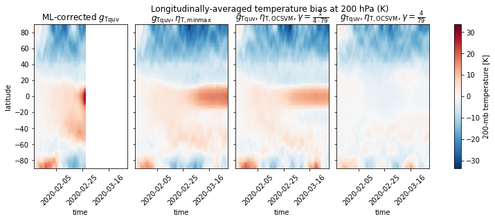
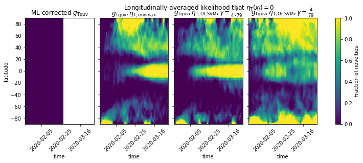
Figure 4: Hovmoller (time vs latitude) plots visualizing projected upper-atmospheric temperature biases (against a fine-grid reference simulation) at the 200hPa pressure level (top) and fractions of novelties identified (bottom) by four different models (left to right): (1) the ML-corrected climate model $g_{\mathrm{Tquv}}$ without novelty detection (which crashes after 38 days), (2) $g_{\mathrm{Tquv}}$ with min-max novelty detection $\eta_{\mathrm{T,minmax}}$, (3) $g_{\mathrm{Tquv}}$ with OCSVM temperature novelty detection $\eta_{\mathrm{T,OCSVM}}$ with small $\gamma=\frac{1}{4\cdot 79}$, and (4) $g_{\mathrm{Tquv}}$ with OCSVM temperature novelty detection $\eta_{\mathrm{T,OCSVM}}$ with large $\gamma=\frac{4}{79}$. (1) crashes due to an increase in upper atmospheric tropic temperatures, while (2) and (3) prevent equatorial temperature increases from spiraling out of control by consistently identifying novelties in that region. (4) identifies these irregularities early enough to prevent the temperature shift outright.

This appendix walks through a specific example of how novelty detection approach prevents a model from crashing. Figure 4 compares the first ten weeks of four ML-corrected simulations: one without novelty detection (equation (2)) and three with novelty detectors (equation (3); a min-max novelty detector and two OCSVMs with different choices of smoothness parameter $\gamma$).

The ML-corrected model without novelty detection crashes after 38 days due to an explosion of equatorial upper-atmospheric temperatures, as viewed in the top-left plot. While the spike in temperatures occurs right before the crash, the model predicted that tropical regions would be hotter than expected before that point. Since tropical regions are among the hottest, this initial heat shift indicates that the predicted temperature columns are likely to be hotter than anything observed in the training dataset.

This narrative is supported by the fact that the models with min-max and OCSVM with $\gamma=\frac{1}{316}$ novelty detectors do not crash. Both are faced with heated equatorial columns at the beginning of the simulation, and those are identified as out-of-sample by both novelty detectors before the aforementioned temperature spike (see the bottom plots). By removing the ML-corrected nudge from the equatorial region, the equatorial temperature biases are bounded and persist due to nearly every equatorial column being identified as a novelty.

On the other hand, the OCSVM with $\gamma=\frac{4}{79}$ entirely negates the equatorial temperature bias by identifying the shift as a novelty far early in time than any other model. While this approach occasionally identifies some tropical columns as out-of-sample during the run, it can reap the benefits of ML-nudging much of the time near the equator.

Appendix D OCSVM parameter comparison

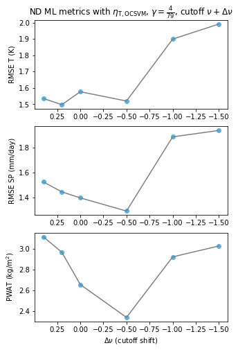
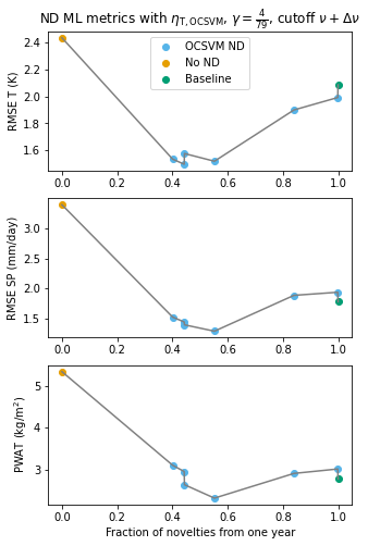
Figure 5: Compares the RMSE of time-averaged 850hPa temperature (top), surface precipitation (center), and precipitable water (bottom) of several year-long simulations of equation (3) with ML-correction $g_{\mathrm{Tquv}}$ and novelty detector $\eta_{\mathrm{T,OCSVM}}$ with $\gamma=\frac{4}{79}$ and cutoff $\nu+\Delta\nu$ where $\nu$ is obtained by equation (4) for $\Delta\nu\in\{-1.5,-1,-0.5,0,0.2,0.4\}$. The left plots show the metric as a function of the cutoff. The right plots instead have the total fraction of novelties identified (which is monotonic as a function of the cutoff) on the x-axis. The right plots additionally feature the the crashed result of the ML-corrected run equation (2) with $g_{\mathrm{Tquv}}$ without novelty detection as a “never-novelty” run and the baseline result of equation (1) as an “always-novelty” run.

Section 3 considers an OCSVM with $\gamma=\frac{4}{d}$ and $\nu$ set to the minimum observed score in the training data and argues that the this model applied to either only temperature or both temperature and humid finds the “sweet spot” between the baseline run and the full ML-corrected run. Here, we validate that conclusion by considering several choices of $\gamma$ and varying $\nu$ to adjust the sensitivity of the novelty detector. We show that these approaches interpolate between the baseline and ML-corrected run as the cutoffs change and that the metrics are optimized by choosing an intermediate model that categorizes a substantial fraction of samples as novelties.

In Figure 5, we consider an ML corrected model $g_{\mathrm{Tquv}}$ augmented with an OCSVM novelty detector $\eta_{\mathrm{T,OCSVM}}$ with $\gamma=\frac{4}{79}$ and various choices of cutoff. When the scalar metrics for evaluating a year-long run are plotted as a function of the cutoff, we find that an intermediate cutoff choice yields optimal performance. We similarly plot these metrics as a function of the fraction of novelties identified by each cutoff and observe a curve with a local minimum that occurs when between 40% and 60% of all samples are deemed novelties. This plot—which includes visualizations of the skill of the crashed ML-corrected run (without novelty detection) and the baseline run—demonstrates that this approach effectively interpolates between those two extreme methods and that the cutoff $\nu$ from equation (4) lies near that sweet spot.

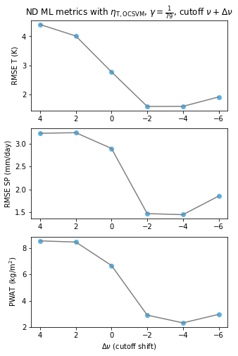
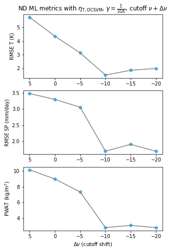
Figure 6: Replicates the experiment visualized in the left panel of Figure 5, but instead considers OCSVM novelty detectors with $\gamma=\frac{1}{79}$ and $\gamma=\frac{1}{316}$ and $\delta\nu\in\{-6,-4,-2,0,2,4\}$ and $\delta\nu\in\{-20,-15,-10,-5,0,5\}$ respectively.

Moreover, this behavior is not isolated to the specific OCSVM considered here and elsewhere in the paper. We train two additional OCSVM models with $\gamma\in\{\frac{1}{79},\frac{1}{316}\}$ and similarly consider a wide range of cutoffs, which are plotted in Figure (6). We find that intermediate choices of the cutoff (at roughly $-4$ and $-10$ respectively) lead to better model RMSE scores on the time-averaged scalar metrics.

References

- [1] V M Krasnopolsky, M S Fox-Rabinovitz, and A A Belochitski. Development of neural network convection parameterizations for numerical climate and weather prediction models using cloud resolving model simulations. In The 2010 International Joint Conference on Neural Networks (IJCNN), pages 1–8, July 2010.
- [2] Noah D. Brenowitz and Christopher S. Bretherton. Spatially extended tests of a neural network parametrization trained by coarse-graining. Journal of Advances in Modeling Earth Systems, 11(8):2728–2744, 2019.
- [3] Oliver Watt-Meyer, Noah D. Brenowitz, Spencer K. Clark, Brian Henn, Anna Kwa, Jeremy McGibbon, W. Andre Perkins, and Christopher S. Bretherton. Correcting weather and climate models by machine learning nudged historical simulations. Geophysical Research Letters, 48(15):e2021GL092555, 2021. e2021GL092555 2021GL092555.
- [4] Janni Yuval and Paul A. O’Gorman. Stable machine-learning parameterization of subgrid processes for climate modeling at a range of resolutions. Nature Communications, 11(1):3295, 2020.
- [5] Stephan Rasp, Michael S. Pritchard, and Pierre Gentine. Deep learning to represent subgrid processes in climate models. Proceedings of the National Academy of Sciences, 115(39):9684–9689, 2018.
- [6] Vladimir M Krasnopolsky, Michael S Fox-Rabinovitz, Hendrik L Tolman, and Alexei A Belochitski. Neural network approach for robust and fast calculation of physical processes in numerical environmental models: Compound parameterization with a quality control of larger errors, 2008.
- [7] Hwan-Jin Song, Soonyoung Roh, and Hyesook Park. Compound parameterization to improve the accuracy of radiation emulator in a numerical weather prediction model. 48(20), October 2021.
- [8] Christopher S. Bretherton, Brian Henn, Anna Kwa, Noah D. Brenowitz, Oliver Watt-Meyer, Jeremy McGibbon, W. Andre Perkins, Spencer K. Clark, and Lucas Harris. Correcting coarse-grid weather and climate models by machine learning from global storm-resolving simulations. Journal of Advances in Modeling Earth Systems, 14(2):e2021MS002794, 2022. e2021MS002794 2021MS002794.
- [9] Guang J. Zhang and Houjun Wang. Toward mitigating the double itcz problem in ncar ccsm3. Geophysical Research Letters, 33(6), 2006.
- [10] M. D. Woelfle, S. Yu, C. S. Bretherton, and M. S. Pritchard. Sensitivity of coupled tropical pacific model biases to convective parameterization in cesm1. Journal of Advances in Modeling Earth Systems, 10(1):126–144, 2018.
- [11] Noah D Brenowitz, Brian Henn, Spencer Clark, Anna Kwa, Jeremy McGibbon, W. Andre Perkins, Oliver Watt-Meyer, and Christopher S. Bretherton. Machine learning climate model dynamics: Offline versus online performance. In NeurIPS 2020 Workshop on Tackling Climate Change with Machine Learning, 2020.
- [12] Spencer K. Clark, Noah D. Brenowitz, Brian Henn, Anna Kwa, Jeremy McGibbon, W. Andre Perkins, Oliver Watt-Meyer, Christopher S. Bretherton, and Lucas M. Harris. Correcting a coarse-grid climate model in multiple climates by machine learning from global 25-km resolution simulations. Earth and Space Science Open Archive, page 46, 2022.
- [13] V.J. Hodge and J. Austin. A survey of outlier detection methodologies. Artificial Intelligence Review, pages 85–126, October 2004. Copyright © 2004 Kluwer Academic Publishers. This is an author produced version of a paper published in Artificial Intelligence Review. This paper has been peer-reviewed but does not include the final publisher proof-corrections or journal pagination.The original publication is available at www.springerlink.com.
- [14] Markus M. Breunig, Hans-Peter Kriegel, Raymond T. Ng, and Jörg Sander. Lof: Identifying density-based local outliers. In Proceedings of the 2000 ACM SIGMOD International Conference on Management of Data, SIGMOD ’00, page 93–104, New York, NY, USA, 2000. Association for Computing Machinery.
- [15] Alexandre Nairac, Neil Townsend, Roy Carr, Steve King, Peter Cowley, and Lionel Tarassenko. A system for the analysis of jet engine vibration data. Integr. Comput.-Aided Eng., 6(1):53–66, jan 1999.
- [16] Stefan Van Aelst and Peter Rousseeuw. Minimum volume ellipsoid. Wiley Interdisciplinary Reviews: Computational Statistics, 1:71 – 82, 07 2009.
- [17] Bernhard Schölkopf, John Platt, John Shawe-Taylor, Alexander Smola, and Robert Williamson. Estimating support of a high-dimensional distribution. Neural Computation, 13:1443–1471, 07 2001.
- [18] Christoph Sommer, Rudolf Hoefler, Matthias Samwer, and Daniel W. Gerlich. A deep learning and novelty detection framework for rapid phenotyping in high-content screening. Molecular Biology of the Cell, 28(23):3428–3436, 2017. PMID: 28954863.
- [19] Somaieh Amraee, Abbas Vafaei, Kamal Jamshidi, and Peyman Adibi. Abnormal event detection in crowded scenes using one-class svm. Signal, Image and Video Processing, 12(6):1115–1123, 2018.
- [20] Yanghui Tan, Chunyang Niu, Hui Tian, Liangsheng Hou, and Jundong Zhang. A one-class svm based approach for condition-based maintenance of a naval propulsion plant with limited labeled data. Ocean Engineering, 193:106592, 2019.
- [21] Kun Yang, Samory Kpotufe, and Nick Feamster. An efficient one-class SVM for anomaly detection in the internet of things. CoRR, abs/2104.11146, 2021.
- [22] IPCC. Summary for Policymakers, pages 3 – 32. Cambridge University Press, Cambridge, United Kingdom and New York, NY, USA, 2021.
- [23] Christopher S. Bretherton, Matthew E. Peters, and Larissa E. Back. Relationships between water vapor path and precipitation over the tropical oceans. Journal of Climate, 17(7):1517 – 1528, 2004.
- [24] Linjiong Zhou, Shian-Jiann Lin, Jan-Huey Chen, Lucas M. Harris, Xi Chen, and Shannon L. Rees. Toward convective-scale prediction within the next generation global prediction system. Bulletin of the American Meteorological Society, 100(7):1225 – 1243, 2019.
- [25] William M. Putman and Shian-Jiann Lin. Finite-volume transport on various cubed-sphere grids. Journal of Computational Physics, 227(1):55–78, 2007.
- [26] Kai-Yuan Cheng, Lucas Harris, Christopher Bretherton, Timothy M. Merlis, Maximilien Bolot, Linjiong Zhou, Alex Kaltenbaugh, Spencer Clark, and Stephan Fueglistaler. Impact of warmer sea surface temperature on the global pattern of intense convection: Insights from a global storm resolving model. Geophysical Research Letters, n/a(n/a):e2022GL099796. e2022GL099796 2022GL099796.