Effects of Backtracking on PageRank

Abstract

In this paper, we consider three variations on standard PageRank: Non-backtracking PageRank, $\mu$-PageRank, and $\infty$-PageRank, all of which alter the standard formula by adjusting the likelihood of backtracking in the algorithm’s random walk. We show that in the case of regular and bipartite biregular graphs, standard PageRank and its variants are equivalent. We also compare each centrality measure and investigate their clustering capabilities.

Keywords: PageRank; random walk; non-backtracking walk.

1 Introduction

Since its development in 1998, the PageRank algorithm has been a powerful tool in search engine optimization [18] and has subsequently been adapted to solve a variety of problems including word sense disambiguation in natural language processing [17], identifying key social media users in social network analysis [12], spam detection in web browsing [11], anomaly detection in movements of seniors [20], among many others. In this paper we explore various variants of PageRank: Non-backtracking PageRank as introduced by Arrigo et. al. [4], $\mu$-PageRank as introduced by Aleja et. al. [1] and Criado et. al. [8], and we introduce a new variant, $\infty$-PageRank. We also investigate the clustering and centrality measure capabilities of PageRank and its variations.

Using iterated random walks, PageRank explores a network of nodes, ranking nodes by the number and quality of connections they have. This algorithm’s ability to process large networks of nodes and identify those of greatest importance or influence makes it applicable in nearly every field with only minor tailoring required to fit the different applications. One such alteration involves swapping the regular random walk used in the algorithm for a non-backtracking random walk. The differences between the two methods are discussed in section 2.1 and 2.2.

Additionally, the numerical emphasis PageRank places on connections between nodes makes it well-suited for use in clustering algorithms. This potential has been thoroughly studied [3, 10, 16]. Researchers found that when compared to other clustering algorithms (k-means, spectral clustering, etc.) PageRank was able to deal more effectively with outliers, non-convex clusters, and high dimensional datasets [16]. We will develop our own clustering algorithm using PageRank variants in Section 4.

A non-backtracking walk on a graph $G$ is a random walk which prohibits immediate backtracking. Non-backtracking random walks are better able to model systems that are unlikely to visit the same node multiple times in a short period. Kitaura et al. [15] suggest that among these networks are models of memory and local awareness. Torres et al. [22] have also used non-backtracking to study target immunization of networks. It is conjectured that the mixing rate (the rate at which the random walk converges to the unique stationary distribution of the graph) of a non-backtracking random walk is faster than that of a simple random walk (a conjecture proved for a variety of cases) [2, 14]. This faster mixing rate allows for computationally efficient sampling of vertices, something that has sparked its use in many other applications including an algorithm to replace the power-of-d choices policy in allocation problems [21], as well as influence maximization [19] and calculation of the clustering coefficient of online social networks [13].

This study of non-backtracking random walks motivates our work on PageRank variants. We build off the work of Arrigo et al. [4], Aleja et al. [1], and Criado et al. [8] to better understand non-backtracking PageRank and $\mu$-PageRank. In Section 2 we will define non-backtracking, and $\mu$-PageRank. In Section 3 we will define $\infty$-PageRank and analyze properties of the the PageRank variants. Then in Section 4 we will define an algorithm for clustering networks based on PageRank and its variants.

2 Standard, Non-Backtracking, and $\mu$-PageRank

2.1 Standard PageRank

Let $G=(V,E)$ be an undirected, unweighted graph with $n$ vertices and $m$ edges. PageRank ranks the nodes of $G$ based on the number of connections a node has and the quality of those connections. It considers a modified random walk $\{v_{1},v_{2},...\}$ across $G$ where, with probability $\epsilon$, $v_{i}$ is chosen uniformly at random from the neighbors of $v_{i-1}$. With probability $1-\epsilon$, $v_{i}$ is chosen from the set of nodes $V$ with probability distribution $u$. The stationary distribution of the modified random walk is the PageRank vector $\pi$ of $G$, where the $i^{th}$ entry of $\pi$ is the PageRank value of node $i$.

Definition 2.1 (PageRank).

Let $G$ be a graph with adjacency matrix $A$ and diagonal degree matrix $D$. Let $\epsilon\in(0,1)$ and $v$ be a initial distribution vector such that $\|v\|_{1}=1$. Then the stationary distribution of

$$P=\epsilon AD^{-1}+(1-\epsilon)u\mathbf{1}^{T}$$

is the PageRank vector $\pi$ of $G$.

Non-backtracking PageRank is the same as PageRank but the random walk step is now a non-backtracking random walk [4, 1]. In order to compare standard and non-backtracking PageRank, we look at an alternative representation of standard PageRank. We define a graph $\hat{G}$ by creating a directed edge $i\rightarrow j$ and $j\rightarrow i$ for every edge $i\sim j$ in $G$ and letting these directed edges be the nodes of $\hat{G}$. Two directed edge $(i,j)$ and $(k,l)$ are connected in $\hat{G}$ if $j=k$. We encapsulate this information in a matrix $C$:

$$C((i,j),(k,l))=\begin{cases}1&j=k\\ 0&j\neq k\end{cases}.$$ (1)

Let $\hat{D}$ be the diagonal degree matrix of $\hat{G}$. Additionally we define the matrices

$$S((i,j),x) =\begin{cases}1&j=x\\ 0&j\neq x\end{cases} T(x,(i,j)) =\begin{cases}1&i=x\\ 0&i\neq x\end{cases}$$ (2)

which are used to project from the vertices of $G$ to its “lifted” edges and vice versa. Arrigo et. al. [4] use these matrices to calculate PageRank of $G$ using the graph $\hat{G}$.

Definition 2.2 (Edge PageRank [4]).

Let $G$ be a graph with lifted graph $\hat{G}$. Let $C$ be the adjacency matrix of $\hat{G}$ and $\hat{D}$ the (edge) degree matrix. Let $u=T^{T}(TT^{T})^{-1}v$ be the initial distribution vector from standard PageRank projected onto $\hat{G}$. Then the stationary distribution of

$$H_{1}=\epsilon C\hat{D}^{-1}+(1-\epsilon)u\mathbf{1}^{T}$$

is the edge PageRank $\hat{\pi}$ of $G$. The PageRank of $G$ is then $\pi=T\hat{\pi}$.

2.2 Non-backtracking PageRank

Using the lift of $G$ onto its directed edges, we can calculate non-backtracking PageRank. To do this we consider the graph created by the non-backtracking matrix defined

$$B((i,j),(k,l))=\begin{cases}1&j=k\text{ and }i\neq l\\ 0&\text{otherwise}\end{cases}.$$

This graph is similar to $\hat{G}$, however edges that backtrack on $G$ do not connect to each other. Note that performing a random walk only the graph generated by $B$ is equivalent to a non-backtracking random walk on the graph $G$. Hence, using $B$ as our adjacency matrix, we can define non-backtracking PageRank in the same manner as Arrigo et. al [4] as follows:

Definition 2.3 (Non-backtracking PageRank [4]).

Let $G$ be a graph with $B$ its non-backtracking matrix and $\hat{D}$ its edge degree matrix. Let $u=T^{T}(TT^{T})^{-1}v$ be the initial distribution vector from standard PageRank projected onto the directed edges of $G$. Then the stationary distribution of

$$H_{0}=\epsilon B^{T}(\hat{D}-I)^{-1}+(1-\epsilon)u\mathbf{1}^{T}$$

is the edge non-backtracking PageRank $\hat{\pi}_{0}$ of $G$. The non-backtracking PageRank of $G$ is $\pi_{0}=T\hat{\pi}_{0}$.

2.3 $\mu$-PageRank

The notion of $\mu$-PageRank (or $\mu$-centrality) has been studied to give an alternative ranking to nodes [1, 8]. The main idea of $\mu$-PageRank is to again perform a modified random walk $\{v_{1},v_{2},...\}$ where $v_{i}$ is chosen at random with probability $\epsilon$ from the neighbors of $v_{i-1}$. However in $\mu$-PageRank, the neighbor from $v_{i-2}$ is weighted by a factor of $\mu$ and all other edges are equally likely to be chosen. Again to encapsulate this modified random walk into a Markov chain by lifting the graph $G$ to a graph of directed edges. We weight every backtracking connection with the probability $\mu$. To do this we define a backtracking operator $\tau$:

$$\tau((i,j),(k,l))=\begin{cases}1&j=k,i=l\\ 0&\text{otherwise}\end{cases}.$$

Intuitively, this is what happens to PageRank as it becomes more or less likely to backtrack in the PageRank modified random walk.

Definition 2.4 ($\mu$-PageRank).

Let $G$ be a graph with $C$ its edge adjacency matrix, $\hat{D}$ its edge degree matrix and $\tau$ the backtracking operator. Let $C_{\mu}=C-(1-\mu)\tau$. Let $u=T^{T}(TT^{T})^{-1}v$ be the initial distribution vector from standard PageRank projected onto the directed edges of $G$. Then the stationary distribution of

$$H_{\mu}=\epsilon C_{\mu}(\hat{D}-(1-\mu)I)^{-1}+(1-\epsilon)u\mathbf{1}^{T}$$

is the edge $\mu$-PageRank $\hat{\pi}_{\mu}$ of $\hat{G}$. The $\mu$-PageRank of $G$ is $\pi_{\mu}=T\hat{\pi}_{\mu}$.

Remark 1.

Aleja et al. and Criado et al. [1, 8] also study $\mu$-PageRank for values $\mu\in[0,1]$. Our study allows $\mu\in[0,\infty)$ to represent random walks where backtracking becomes increasingly likely. This notion will be studied in section 3.2.

Remark 2.

Setting $\mu=1$ weights all the edges the same giving the standard PageRank of $G$. If $\mu=0$, this makes it impossible to choose $v_{i-2}$ as $v_{i}$ with probability $\epsilon$ and is therefore non-backtracking PageRank. This motivates the notation $H_{1}$ and $H_{0}$ for standard and non-backtracking PageRank respectively.

3 Analysis of $\mu$-PageRank

Given the versatility of $\mu$-pagerank, analyzing $\mu$-pagerank can lead to insights for both non-backtracking and standard PageRank. In this section, we will prove general properties $\mu$-PageRank. We will also calculate the limiting value of $\mu$-PageRank as $\mu\rightarrow\infty$, defining the notion of $\infty$-PageRank. We will end the section discussing conjectures about the implications of $\infty$-PageRank.

3.1 $\mu$-PageRank of Regular Graphs and Biregular Bipartite Graphs

With the same methodology as Arrigo et al. [4], we can prove a more general result of their Theorem 4:

Theorem 3.1.

Let $A$ be the adjacency matrix of an undirected $k$-regular connected graph with $k\geq 2$. Then for $\epsilon\in[0,1]$, define the matrices $H_{\mu}$, $H_{1}$ and $T$ as before. Then if $H_{\mu}^{T}\hat{\mathbf{y}}=\hat{\mathbf{y}}$ and $H_{1}^{T}\hat{\mathbf{x}}=\hat{\mathbf{x}}$ with $\|\hat{\mathbf{x}}\|=\|\hat{\mathbf{y}}\|=1$, then we have $T\hat{\mathbf{y}}=T\hat{\mathbf{x}}$.

Proof.

The proof follows in an identical manner to Theorem 4 in [4] with $H_{\mu}$ in place of $H_{0}$. ∎

We can further extend the result to bipartite biregular graphs.

Theorem 3.2.

Let $A$ be the adjacency matrix of an undirected bipartite biregular connected graph with $d_{1},d_{2}\geq 2$ where $d_{i}$ is the degree of each node in the $i^{th}$ part. Then for $\epsilon\in[0,1]$, define the matrices $H_{\mu}$, $H_{1}$ and $T$ as before. If $H_{1}^{T}\hat{\mathbf{x}}=\hat{\mathbf{x}}$ and $H_{\mu}^{T}\hat{\mathbf{y}}=\hat{\mathbf{y}}$, and $\|\hat{\mathbf{x}}\|=\|\hat{\mathbf{y}}\|=1$, then $T\hat{\mathbf{y}}=T\hat{\mathbf{x}}$.

Proof.

Since $G$ is bipartite, we can write

$$C_{\mu}=\begin{pmatrix}0&C_{2}\\ C_{1}&0\end{pmatrix} T=\begin{pmatrix}T_{1}&0\\ 0&T_{2}\end{pmatrix}.$$

We can solve for $\hat{\mathbf{y}}$ by solving

$$\Biggl{(}\begin{pmatrix}I_{1}&0\\ 0&I_{2}\end{pmatrix}-\epsilon\begin{pmatrix}0&C_{1}^{T}\\ C_{2}^{T}&0\end{pmatrix}\begin{pmatrix}\frac{1}{d_{2}-(1-\mu)}&0\\ 0&\frac{1}{d_{1}-(1-\mu)}\end{pmatrix}\Biggr{)}\hat{\mathbf{y}}=\frac{1-\epsilon}{n}\begin{pmatrix}T_{1}^{T}&0\\ 0&T_{2}^{T}\end{pmatrix}\begin{pmatrix}\frac{1}{d_{1}}&0\\ 0&\frac{1}{d_{2}}\end{pmatrix}\mathbf{1}.$$

Recall that $T$ is the out degree matrix. Thus $T^{T}\mathbf{1}$ counts the number of nodes which point to a certain edge (the edge in-degree). Note that edges can only have one node pointing to them. So $T^{T}\mathbf{1}=\mathbf{1}$. We can then simplify the right side of the equation to

$$\frac{1-\epsilon}{n}\begin{pmatrix}T_{1}^{T}&0\\ 0&T_{2}^{T}\end{pmatrix}\begin{pmatrix}\frac{1}{d_{1}}&0\\ 0&\frac{1}{d_{2}}\end{pmatrix}\mathbf{1}=\frac{1-\epsilon}{n}\begin{pmatrix}\frac{1}{d_{1}}T_{1}^{T}&0\\ 0&\frac{1}{d_{2}}T_{2}^{T}\end{pmatrix}\mathbf{1}=\frac{1-\epsilon}{n}\begin{pmatrix}\frac{1}{d_{1}}\mathbf{1}\\ \frac{1}{d_{2}}\mathbf{1}\end{pmatrix}.$$

We use the inverse of the matrix on the left side of the equation to get

$$\hat{\mathbf{y}}=\frac{1-\epsilon}{n}\Biggl{(}\begin{pmatrix}I_{1}&0\\ 0&I_{2}\end{pmatrix}-\alpha\begin{pmatrix}0&\frac{1}{d_{1}-1}C_{1}^{T}\\ \frac{1}{d_{2}-1}C_{2}^{T}\end{pmatrix}\Biggr{)}^{-1}\begin{pmatrix}\frac{1}{d_{1}}\mathbf{1}\\ \frac{1}{d_{2}}\mathbf{1}\end{pmatrix}.$$

We replace the inverse matrix with the geometric series.

$$\hat{\mathbf{y}} =\frac{1-\epsilon}{n}\left(\sum_{r=0}^{\infty}\epsilon^{r}\begin{pmatrix}0&\frac{1}{d_{1}-(1-\mu)}C_{1}^{T}\\ \frac{1}{d_{2}-(1-\mu)}C_{2}^{T}&0\end{pmatrix}^{r}\right)\begin{pmatrix}\frac{1}{d_{1}}\mathbf{1}\\ \frac{1}{d_{2}}\mathbf{1}\end{pmatrix}.$$

By induction, we can rewrite this sum based on the even and odd values of $r$. When we do this, we have the matrices

$$J_{1} =\begin{pmatrix}\Bigl{(}\frac{1}{(d_{1}-(1-\mu))(d_{2}-(1-\mu))}C_{1}^{T}C_{2}^{T}\Bigr{)}^{r}&0\\ 0&\Bigl{(}\frac{1}{(d_{1}-(1-\mu))(d_{2}-(1-\mu))}C_{2}^{T}C_{1}^{T}\Bigr{)}^{r}\end{pmatrix}$$

$$J_{2} =\begin{pmatrix}0&\frac{1}{d_{1}-(1-\mu)}C_{1}^{T}\Bigl{(}\frac{1}{(d_{1}-(1-\mu))(d_{2}-(1-\mu))}C_{2}^{T}C_{1}^{T}\Bigr{)}^{r}\\ \frac{1}{d_{2}-(1-\mu)}C_{2}^{T}\Bigr{(}\frac{1}{(d_{1}-(1-\mu))(d_{2}-(1-\mu))}C_{1}^{T}C_{2}^{T}\Bigr{)}^{r}&0\end{pmatrix}$$

corresponding with the even and odd terms respectively. This gives the PageRank equation

$$\hat{\mathbf{y}}= \frac{1-\epsilon}{n}\Biggl{(}\sum_{r=0}^{\infty}\epsilon^{2r}J_{1}\begin{pmatrix}\frac{1}{d_{1}}\mathbf{1}\\ \frac{1}{d_{2}}\mathbf{1}\end{pmatrix}+\sum_{r=0}^{\infty}\epsilon^{2r+1}J_{2}\begin{pmatrix}\frac{1}{d_{1}}\mathbf{1}\\ \frac{1}{d_{2}}\mathbf{1}\end{pmatrix}\Biggr{)}$$

$$= \frac{1-\epsilon}{n}\Biggl{(}\sum_{r=0}^{\infty}\epsilon^{2r}\begin{pmatrix}\frac{1}{d_{1}}\Bigl{(}\frac{1}{(d_{1}-(1-\mu))(d_{2}-(1-\mu))}C_{1}^{T}C_{2}^{T}\Bigr{)}^{r}\mathbf{1}\\ \frac{1}{d_{2}}\Bigl{(}\frac{1}{(d_{1}-(1-\mu))(d_{2}-(1-\mu))}C_{2}^{T}C_{1}^{T}\Bigr{)}^{r}\mathbf{1}\end{pmatrix}$$

$$+\sum_{r=0}^{\infty}\epsilon^{2r+1}\begin{pmatrix}\frac{1}{d_{2}(d_{1}-(1-\mu))}C_{1}^{T}\Bigl{(}\frac{1}{(d_{1}-(1-\mu))(d_{2}-(1-\mu))}C_{2}^{T}C_{1}^{T}\Bigr{)}^{r}\mathbf{1}\\ \frac{1}{d_{1}(d_{2}-(1-\mu))}C_{2}^{T}\Bigr{(}\frac{1}{(d_{1}-(1-\mu))(d_{2}-(1-\mu))}C_{1}^{T}C_{2}^{T}\Bigr{)}^{r}\mathbf{1}\end{pmatrix}\Biggr{)}.$$

Note that $G$ is biregular and $C_{1}$ is an adjacency matrix mapping edges from partition 1 to edges from partition 2 (similarly $C_{2}$ maps from 2 to 1). Thus, $C_{1}^{T}\mathbf{1}$ will count the number of incoming edges to partition 1 from partition 2. This is the same as counting the number of edges leaving a node from partition 1 to partition 2 (the degree of nodes in partition 1). Thus, $C_{1}^{T}\mathbf{1}=(d_{1}-(1-\mu))\mathbf{1}$. Similarly $C_{2}^{T}\mathbf{1}=(d_{2}-(1-\mu))\mathbf{1}$. Thus,

$$\hat{\mathbf{y}}= \frac{1-\epsilon}{n}\Biggl{(}\sum_{r=0}^{\infty}\epsilon^{2r}\begin{pmatrix}\frac{1}{d_{1}}\Bigl{(}\frac{(d_{1}-(1-\mu))(d_{2}-(1-\mu))}{(d_{1}-(1-\mu))(d_{2}-(1-\mu))}\mathbf{1}\Bigr{)}^{r}\\ \frac{1}{d_{2}}\Bigl{(}\frac{(d_{1}-(1-\mu))(d_{2}-(1-\mu))}{(d_{1}-(1-\mu))(d_{2}-(1-\mu))}\mathbf{1}\Bigr{)}^{r}\end{pmatrix}$$

$$+\sum_{r=0}^{\infty}\epsilon^{2r+1}\begin{pmatrix}\frac{1}{d_{2}(d_{1}-(1-\mu))}C_{1}^{T}\Bigl{(}\frac{(d_{1}-(1-\mu))(d_{2}-(1-\mu))}{(d_{1}-(1-\mu))(d_{2}-(1-\mu))}\mathbf{1}\Bigr{)}^{r}\\ \frac{1}{d_{1}(d_{2}-(1-\mu))}C_{2}^{T}\Bigr{(}\frac{(d_{1}-(1-\mu))(d_{2}-(1-\mu))}{(d_{1}-(1-\mu))(d_{2}-(1-\mu))}\mathbf{1}\Bigr{)}^{r}\end{pmatrix}\Biggr{)}$$

$$= \frac{1-\epsilon}{n}\Biggl{(}\sum_{r=0}^{\infty}\epsilon^{2r}\begin{pmatrix}\frac{1}{d_{1}}\mathbf{1}\\ \frac{1}{d_{2}}\mathbf{1}\end{pmatrix}+\sum_{r=0}^{\infty}\epsilon^{2r+1}\begin{pmatrix}\frac{1}{d_{2}(d_{1}-(1-\mu))}C_{1}^{T}\mathbf{1}\\ \frac{1}{d_{1}(d_{2}-(1-\mu))}C_{2}^{T}\mathbf{1}\end{pmatrix}\Biggr{)}$$

$$= \frac{1-\epsilon}{n}\Biggl{(}\sum_{r=0}^{\infty}\epsilon^{2r}\begin{pmatrix}\frac{1}{d_{1}}\mathbf{1}\\ \frac{1}{d_{2}}\mathbf{1}\end{pmatrix}+\sum_{r=0}^{\infty}\epsilon^{2r+1}\begin{pmatrix}\frac{1}{d_{2}}\mathbf{1}\\ \frac{1}{d_{1}}\mathbf{1}\end{pmatrix}\Biggr{)}$$

$$= \frac{1-\epsilon}{n}\Biggl{(}\begin{pmatrix}\Bigl{(}\sum_{r=0}^{\infty}\frac{(\epsilon^{2})^{r}}{d_{1}}\Bigr{)}\mathbf{1}\\ \Bigl{(}\sum_{r=0}^{\infty}\frac{(\epsilon^{2})^{r}}{d_{2}}\Bigr{)}\mathbf{1}\end{pmatrix}+\begin{pmatrix}\Bigl{(}\sum_{r=0}^{\infty}\frac{\epsilon^{2r+1}}{d_{2}}\Bigr{)}\mathbf{1}\\ \Bigl{(}\sum_{r=0}^{\infty}\frac{\epsilon^{2r+1}}{d_{1}}\Bigr{)}\mathbf{1}\end{pmatrix}\Biggr{)}$$

$$= \frac{1-\epsilon}{n}\Biggl{(}\begin{pmatrix}\frac{1}{d_{1}}\Bigl{(}\sum_{r=0}^{\infty}(\epsilon^{2})^{r}\Bigr{)}\mathbf{1}\\ \frac{1}{d_{2}}\Bigl{(}\sum_{r=0}^{\infty}(\epsilon^{2})^{r}\Bigr{)}\mathbf{1}\end{pmatrix}+\begin{pmatrix}\frac{1}{d_{2}}\Bigl{(}\sum_{r=0}^{\infty}\epsilon^{2r+1}\Bigr{)}\mathbf{1}\\ \frac{1}{d_{1}}\Bigl{(}\sum_{r=0}^{\infty}\epsilon^{2r+1}\Bigr{)}\mathbf{1}\end{pmatrix}\Biggr{)}$$

$$= \frac{1-\epsilon}{n}\Biggl{(}\begin{pmatrix}\frac{1}{d_{1}}\Bigl{(}\sum_{r=0}^{\infty}(\epsilon^{2})^{r}\Bigr{)}\mathbf{1}\\ \frac{1}{d_{2}}\Bigl{(}\sum_{r=0}^{\infty}(\epsilon^{2})^{r}\Bigr{)}\mathbf{1}\end{pmatrix}+\begin{pmatrix}\frac{\epsilon}{d_{2}}\Bigl{(}\sum_{r=0}^{\infty}\epsilon^{2r}\Bigr{)}\mathbf{1}\\ \frac{\epsilon}{d_{1}}\Bigl{(}\sum_{r=0}^{\infty}\epsilon^{2r}\Bigr{)}\mathbf{1}\end{pmatrix}\Biggr{)}$$

$$= \frac{1-\epsilon}{n}\Biggl{(}\begin{pmatrix}\Bigl{(}\frac{1}{d_{1}}+\frac{\epsilon}{d_{2}}\Bigr{)}\Bigl{(}\sum_{r=0}^{\infty}(\epsilon^{2})^{r}\Bigr{)}\mathbf{1}\\ \Bigl{(}\frac{1}{d_{2}}+\frac{\epsilon}{d_{1}}\Bigr{)}\Bigl{(}\sum_{r=0}^{\infty}(\epsilon^{2})^{r}\Bigr{)}\mathbf{1}\end{pmatrix}\Biggr{)}.$$

Since $\epsilon^{2}<1$, the summation converges to $\frac{1}{1-\epsilon^{2}}$. Further, we simplify the fractions and get

$$\hat{\mathbf{y}} =\frac{1-\epsilon}{n}\Biggl{(}\begin{pmatrix}\Bigl{(}\frac{d_{2}+\epsilon d_{1}}{d_{1}d_{2}}\Bigr{)}\Bigl{(}\frac{1}{1-\epsilon^{2}}\Bigr{)}\mathbf{1}\\ \Bigl{(}\frac{d_{1}+\epsilon d_{2}}{d_{1}d_{2}}\Bigr{)}\Bigl{(}\frac{1}{1-\epsilon^{2}}\Bigr{)}\mathbf{1}\end{pmatrix}\Biggr{)}$$

$$=\frac{1-\epsilon}{nd_{1}d_{2}(1-\epsilon^{2})}\begin{pmatrix}(d_{2}+\epsilon d_{1})\mathbf{1}\\ (d_{1}+\epsilon d_{2})\mathbf{1}\end{pmatrix}$$

$$=\frac{1}{nd_{1}d_{2}(1+\epsilon)}\begin{pmatrix}(d_{2}+\epsilon d_{1})\mathbf{1}\\ (d_{1}+\epsilon d_{2})\mathbf{1}\end{pmatrix}.$$

Now to project $\hat{\mathbf{y}}$ to the vertex space, we get

$$T\hat{\mathbf{y}} =\frac{1}{nd_{1}d_{2}(1+\epsilon)}\begin{pmatrix}T_{1}&0\\ 0&T_{2}\end{pmatrix}\begin{pmatrix}(d_{2}+\epsilon d_{1})\mathbf{1}\\ (d_{1}+\epsilon d_{2})\mathbf{1}\end{pmatrix}$$

$$=\frac{1}{nd_{1}d_{2}(1+\epsilon)}\begin{pmatrix}(d_{2}+\epsilon d_{1})(T_{1}\mathbf{1})\\ (d_{1}+\epsilon d_{2})(T_{2}\mathbf{1})\end{pmatrix}.$$

Note that $T\mathbf{1}$ counts the number of outgoing edges from a given node. Thus, $T_{1}\mathbf{1}=d_{1}$ and $T_{2}\mathbf{1}=d_{2}$. Thus,

$$T\hat{\mathbf{y}} =\frac{1}{nd_{1}d_{2}(1+\epsilon)}\begin{pmatrix}(d_{2}+\epsilon d_{1})d_{1}\mathbf{1}\\ (d_{1}+\epsilon d_{2})d_{2}\mathbf{1}\end{pmatrix}$$

$$=\frac{1}{n(1+\epsilon)}\begin{pmatrix}1+\epsilon\frac{d_{1}}{d_{2}}&0\\ 0&1+\epsilon\frac{d_{2}}{d_{1}}\end{pmatrix}\mathbf{1}.$$

Recall that in a bipartite, biregular graph, the adjacency matrix is $A=\begin{pmatrix}0&A_{1}\\ A_{2}&0\end{pmatrix}.$ Thus

$$\mathbf{x} =\frac{1-\epsilon}{n}(I-\alpha AD^{-1})^{-1}\mathbf{1}$$

$$=\frac{1-\epsilon}{n}\Bigl{(}\sum_{r=0}^{\infty}\epsilon^{r}(A)^{r}(D^{-1})^{r}\Bigr{)}\mathbf{1}$$

$$=\frac{1-\epsilon}{n}\Bigl{(}\sum_{r=0}^{\infty}\epsilon^{r}\begin{pmatrix}0&A_{2}^{T}\\ A_{1}^{T}&0\end{pmatrix}^{r}\begin{pmatrix}\frac{1}{d_{2}}&0\\ 0&\frac{1}{d_{2}}\end{pmatrix}^{r}\Bigr{)}\mathbf{1}$$

$$=\frac{1-\epsilon}{n}\Bigl{(}\sum_{r=0}^{\infty}\epsilon^{r}\begin{pmatrix}0&\frac{A_{2}^{T}}{d_{1}}\\ \frac{A_{1}^{T}}{d_{2}}&0\end{pmatrix}^{r}\Bigr{)}\mathbf{1}$$

$$=\frac{1-\epsilon}{n}\Bigl{(}\sum_{r=0}^{\infty}\epsilon^{2r}\begin{pmatrix}(\frac{A_{1}^{T}A_{2}^{T}}{d_{1}d_{2}})^{r}&0\\ 0&(\frac{A_{2}^{T}A_{1}^{T}}{d_{1}d_{2}})^{r}\end{pmatrix}+\sum_{r=0}^{\infty}\epsilon^{2r+1}\begin{pmatrix}0&\frac{A_{2}^{T}}{d_{1}}(\frac{A_{2}^{T}A_{1}^{T}}{d_{1}d_{2}})^{r}\\ \frac{A_{1}^{T}}{d_{2}}(\frac{A_{1}^{T}A_{2}^{T}}{d_{1}d_{2}})^{r}&0\end{pmatrix}\Bigr{)}\mathbf{1}$$

$$=\frac{1-\epsilon}{n}\Bigl{(}\sum_{r=0}^{\infty}\epsilon^{2r}\begin{pmatrix}(\frac{A_{1}^{T}A_{2}^{T}}{d_{1}d_{2}})^{r}\mathbf{1}\\ (\frac{A_{2}^{T}A_{1}^{T}}{d_{2}d_{1}})^{r}\mathbf{1}\end{pmatrix}+\sum_{r=0}^{\infty}\epsilon^{2r+1}\begin{pmatrix}\frac{A_{2}^{T}}{d_{1}}(\frac{A_{2}^{T}A_{1}^{T}}{d_{2}d_{1}})^{r}\mathbf{1}\\ \frac{A_{1}^{T}}{d_{2}}(\frac{A_{1}^{T}A_{2}^{T}}{d_{1}d_{2}})^{r}\mathbf{1}\end{pmatrix}\Bigr{)}$$

$$=\frac{1-\epsilon}{n}\Bigl{(}\sum_{r=0}^{\infty}\epsilon^{2r}\mathbf{1}+\sum_{r=0}^{\infty}\epsilon^{2r+1}\begin{pmatrix}\frac{d_{2}}{d_{1}}\\ \frac{d_{1}}{d_{2}}\end{pmatrix}\mathbf{1}\Bigr{)}$$

$$=\frac{1-\epsilon}{n}\Bigl{(}\sum_{r=0}^{\infty}\epsilon^{2r}\mathbf{1}+\epsilon\sum_{r=0}^{\infty}\epsilon^{2r}\begin{pmatrix}\frac{d_{2}}{d_{1}}\\ \frac{d_{1}}{d_{2}}\end{pmatrix}\mathbf{1}\Bigr{)}$$

$$=\frac{1-\epsilon}{n(1-\epsilon^{2})}\Bigl{(}\begin{pmatrix}1+\epsilon\frac{d_{2}}{d_{1}}\\ 1+\epsilon\frac{d_{1}}{d_{2}}\end{pmatrix}\mathbf{1}\Bigr{)}$$

$$=\frac{1}{n(1+\epsilon)}\begin{pmatrix}1+\epsilon\frac{d_{2}}{d_{1}}&0\\ 0&1+\epsilon\frac{d_{1}}{d_{2}}\end{pmatrix}\mathbf{1}.$$

Thus, $T\hat{\mathbf{y}}=\mathbf{x}=T\hat{\mathbf{x}}$. ∎

Remark 3.

Applying Theorem 3.2 with $\mu=1$ and $\mu=0$, we have the bipartite biregular graphs result in equivalent PageRank values for standard and non-backtracking PageRank.

3.2 Limit as $\mu\rightarrow\infty$

Most commonly $\mu$-PageRank is studied for $\mu\in[0,1]$ (see [1, 8]). However we can easily extend the domain of $\mu$ to be $[0,\infty)$. Intuitively, as $\mu$ gets larger it becomes more and more likely to backtrack with probability $\epsilon$ in the modified random walk. Thus as $\mu\rightarrow\infty$, we approach the $\infty$-PageRank of the graph $G$ (or the ranking of nodes if with probability $\epsilon$ we bounce back and forth between two nodes). This limit can be calculated explicitly.

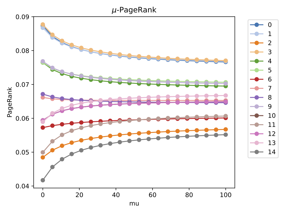
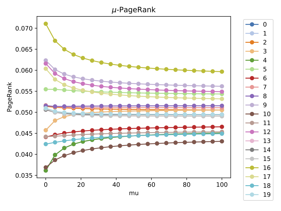
Figure 1: The first plot depicts the PageRank values of a 14-node graph over 20 different values of $\mu$ spanning from 0 to 100. The second plot depicts the same data for a 19-node graph.

Proposition 3.3 ($\infty$-PageRank).

Let $G$ be a graph with initial distribution vector $v$ and $\mu$-PageRank as in Definition 2.4. Let $\pi_{\infty}=\lim_{\mu\rightarrow\infty}\pi_{\mu}$ be the $\infty$-PageRank of $G$. Then

$$\pi_{\infty} =(1+\epsilon)^{-1}v+\epsilon(1+\epsilon)^{-1}AD^{-1}v.$$

Therefore the $\infty$-PageRank of node $i$ is $\frac{v_{i}}{1+\epsilon}+\frac{\epsilon}{1+\epsilon}\sum_{j\sim i}\frac{v_{j}}{d_{j}}$ where $d_{j}$ is the degree of node $j$.

Proof.

For $\epsilon\in(0,1)$ we have

$$H_{\infty} =\lim_{\mu\rightarrow\infty}\epsilon C_{\mu}(\hat{D}-(1-\mu)I)^{-1}+(1-\epsilon)u\mathbf{1}^{T}$$ (3)

$$=\epsilon\tau+(1-\epsilon)u\mathbf{1}^{T}.$$ (4)

Then we have

$$\hat{\pi}_{\infty} =\epsilon\tau\hat{\pi}_{\infty}+(1-\epsilon)u\mathbf{1}^{T}\hat{\pi}_{\infty}$$ (5)

$$(I-\epsilon\tau)\hat{\pi}_{\infty} =(1-\epsilon)T^{T}(TT^{T})^{-1}v$$ (6)

$$\hat{\pi}_{\infty} =(1-\epsilon)(I-\epsilon\tau)^{-1}T^{T}(TT^{T})^{-1}v.$$ (7)

Direct computation shows that $(I-\epsilon\tau)^{-1}=(1-\epsilon^{2})^{-1}I+\frac{\epsilon}{1-\epsilon^{2}}\tau$. So

$$\hat{\pi}_{\infty}=\Big{(}(1+\epsilon)^{-1}I+\epsilon(1+\epsilon)^{-1}\tau\Big{)}T^{T}(TT^{T})^{-1}v.$$

To project onto the nodes of $G$, we left multiply by $T$. To simplify this computation, we use the facts that $TT^{T}=D$, $T\tau=S^{T}$ and $TS=A$. This gives

$$\pi_{\infty} =(1+\epsilon)^{-1}TT^{T}(TT^{T})^{-1}v+\epsilon(1+\epsilon)^{-1}T\tau T^{T}(TT^{T})^{-1}v$$ (8)

$$=(1+\epsilon)^{-1}v+\epsilon(1+\epsilon)^{-1}AD^{-1}v.$$ (9)

∎

Unsurprisingly, the $\infty$-PageRank of a node only depends upon the degree of its neighbors. It is worth noting that this limit can be calculated extremely quickly.

3.3 Monotonicity

We conjecture that $\mu$-PageRank is a monotonic function. We also conjecture that the range of values of $\mu$-PageRank shrinks as $\mu\rightarrow\infty$. To test this conjecture, we generated a stochastic block model graph and calculated the $\mu$-PageRank centrality values of the graph for 20 different values of $\mu$ between 0 and 100. This simulates taking the limit as $\mu$ goes to infinity as we have seen most graphs of this nature have $\mu$-PageRank empirically converge to their limit before 100. This produces the plots seen in Figure 1. We can then take the differences between the $\mu$-PageRank values and determine if all the differences have the same sign. Taking into account machine error, our analysis leads us to the following conjecture:

Conjecture 3.1.

The function $(\pi_{\mu})_{i}$ is monotonic for all $i$ and

$$\max_{i}\pi_{\mu}(i)-\min_{i}\pi_{\mu}(i)\leq\max_{i}\pi_{\mu+\alpha}(i)-\min_{i}\pi_{\mu+\alpha}(i)$$

for all $\alpha>0$.

If this conjecture holds, it leads to computationally efficient comparisons between standard and non-backtracking PageRank. Specifically, one can compare $\infty$-PageRank with standard PageRank to determine whether the non-backtracking PageRank of a node is greater or lesser than standard PageRank. Due to the computational complexity of calculating non-backtracking PageRank, this can create a quick comparison between the node standard and non-backtracking PageRank values and rankings.

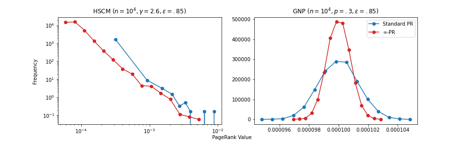
Figure 2: The left plot is an HSCM random network with $10^{4}$ nodes. The right plot is a GNP random graph with $10^{4}$ nodes. The blue represents the distribution of standard PageRank values and the red represents the distribution of $\infty$-PageRank values. We see that in the cases of scale free networks, the $\infty$-PageRank distribution is similar to its standard counterparts.

3.4 Top Nodes in $\infty$-PageRank and Standard PageRank

Due to precision error, the exact PageRank value of a node is often not as informative as the nodes ranking in comparison to other vertices in the network. As such, we investigate how the top nodes of standard PageRank compare with the top nodes of $\infty$-PageRank. This is motivated by the computational efficiency of computing $\infty$-PageRank.

Many real-world networks exhibit scale-free behavior [6, 7]. That is, the degrees of the nodes are drawn from a heavy-tailed distribution. The standard PageRank of scale-free networks has been previously studied [5, 9]. In fact, [9] finds if the degree distribution is heavy-tailed, the PageRank will also be heavy-tailed. Given the similarity in dependence on the degree distribution of $\infty$-PageRank, we expect similar results (see Figure 2).

Conjecture 3.2.

If $d_{i}\sim X$ where $X$ is a regularly-varying random variable and $d_{i}$ is the degree of node $i\in V(G)$, then $PR_{\infty}(i)$ will also be scale-free.

We further hypothesize these distributions will mirror each other. To test this, we measure the overlap of top nodes in each PageRank distribution. We test this on random graphs and on scale-free networks generated by a hyper-soft configuration model based on a Pareto distribution [23]. As seen in Figure 3, we find high overlap for scale-free networks consistently. This result does not hold for random graphs.

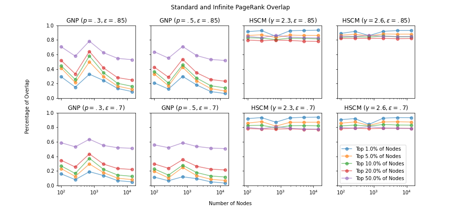
Figure 3: Each plot compares the percentage of nodes which occur in the top $x$ percent of PageRank values for both standard and infinite PageRank. The lines in each plot represent different values of $x$ ($1,5,10,$ and $20$). Each network model is generated 100 times and then the overlap in the top $x$% of nodes is compared for each iteration. These percentages are then averaged across network size. The distribution of the percentages across the 100 iterations was normally distributed with low variance.

4 Clustering with $\infty$-PageRank

To test the clustering capabilities of $\infty$-PageRank, we altered the algorithm PageRank-ClusteringA developed by Chung et al. [10] to create an algorithm capable of $\infty$-PageRank clustering. In this process, we begin with a graph $G$ and its vertex set $V(G)$. We then define an error tolerance value $tol$ that will determine when the algorithm has converged sufficiently for our needs, a jumping factor $\alpha\in(0,1)$ and a personalization vector $v_{n}$ for each node $n\in V(G)$. In our experiments, we use $v_{n}=e_{n}$ where $u_{n}$ is the $n$th standard unit vector. Now for each node, we compute

$$\rho_{n}=\rho_{\infty}(n,v_{n})=(1+(1-\alpha))^{-1}v_{n}+(1-\alpha)(1+(1-\alpha))^{-1}AD^{-1}v_{n}$$

This is the $\infty$-PageRank vector for the node $n$ using personalization vector $v_{n}$. From here, we randomly choose $k$ centers and assemble their PageRank vectors {$\rho_{n}$ for $n\in C_{k}$} into a matrix $\Gamma$ where $\Gamma_{i}$ is a PageRank vector $\rho_{n}$. We are now ready to begin sorting the remaining $n-k$ nodes into our $k$ clusters. For each node $n$ we compute the PageRank Distance of that node to each of the centers $\Gamma_{i}$ which is defined in [10] as

$$\text{distance}_{n,i}=||\rho_{n}D^{-1/2}-\Gamma_{i}D^{-1/2}||$$

From here we define a list of node labels $L$. The label of a node $n$ is determined by the value of $i$ which minimizes $\text{distance}_{n,i}$. We now redefine $\Gamma_{i}$ as the average of the PageRank vectors {$\rho_{n}$|$L_{n}=i$}, and we restart the iteration with our newly defined $\Gamma$. The iteration ends when the error between the previous version of $\Gamma$ and the most recent version of $\Gamma$ (which we will call $\Omega$) is within the tolerance we set at the beginning. At the end of the iteration, the labels assigned by $L$ are considered to be our final label estimates. The pseudocode for this process is given in Algorithm 1.

Algorithm 1 $\infty$-PageRank Clustering Algorithm

$V(G)\leftarrow$ Vertex set of Graph;$\triangleright$ Initialize Variables

$k\leftarrow$ Number of Clusters;

$tol\leftarrow$ Tolerance for Error;

$v_{n}\leftarrow$ Personalization vector for node $n$;

$L\leftarrow$ Collection of node labels;

for $n$ in $V(G)$ do

     $\rho_{n}\leftarrow\rho_{\infty}(n,v_{n})$ $\triangleright$ Calculate infinite PageRank with $v_{n}$

end for

$\Gamma\leftarrow$ PageRank vectors of $k$ randomly selected nodes

error $\leftarrow\infty$

while error $<tol$ do

     for $n$ in $G$ do

         distances$\leftarrow[0,0,...]$$\triangleright$ Initialize list of distances of size $k$

         for $i$ in range($k$) do

              $\text{distance}_{i}\leftarrow\text{dist}(\rho_{n},\Gamma_{i})$ $\triangleright$ Calculate PR-dist between node’s PageRank vector and each cluster center

         end for

         $L_{n}\leftarrow\text{argmin}(\text{distances})$$\triangleright$ Label node based on which center it is closest to

     end for

     $C_{i}\leftarrow$Collection of PageRank vectors of nodes with label $i$

     $\Omega_{i}\leftarrow$Zero array of size $k$

     for $i$ in range($k$) do

         $\Omega_{i}\leftarrow\text{ Average}(C_{i})$$\triangleright$ Calculate new cluster centers

     end for

     error $\leftarrow\|\Gamma-\Omega\|$$\triangleright$ Calculate difference in old and new cluster centers

     $\Gamma\leftarrow\Omega$ $\triangleright$ Update centers

end while

We tested this algorithm on stochastic block matrices and the network containing 114 NCAA Division I American collegiate football teams, connected by the schools that had played against each other. We will first discuss the outcome of the randomly generated stochastic block matrices. These were created by specifying a graph with $k$ clusters containing $n_{i}$ nodes in the $i$th cluster. The main metric we consider here is $c_{in}-c_{out}$, where $c_{in}$ is the number of inter-cluster connections and $c_{out}$ is the number of outer-cluster connections. So when $c_{in}-c_{out}=0$, it is equally likely for the node to be connected to a node within its cluster as it is to be connected to a node outside of its cluster. The lower $c_{in}-c_{out}$ values describe graphs without clear boundaries between clusters, making the clusters harder to detect. In Figure 4, we show a SBM network with $c_{in}-c_{out}=0.8$ with the correct labels and with the clustering labels. Of the 90 nodes in this graph, approximately 89 were correctly clustered, giving an accuracy of 0.98. In total, we ran 450 clustering trials on randomly generated stochastic block matrices, and we charted the relationship between $c_{in}-c_{out}$ values and clustering algorithm accuracy (see Figure 4). We see that there is almost a logarithmic relationship between the $c_{in}-c_{out}$ values and the accuracy of the clustering algorithm.

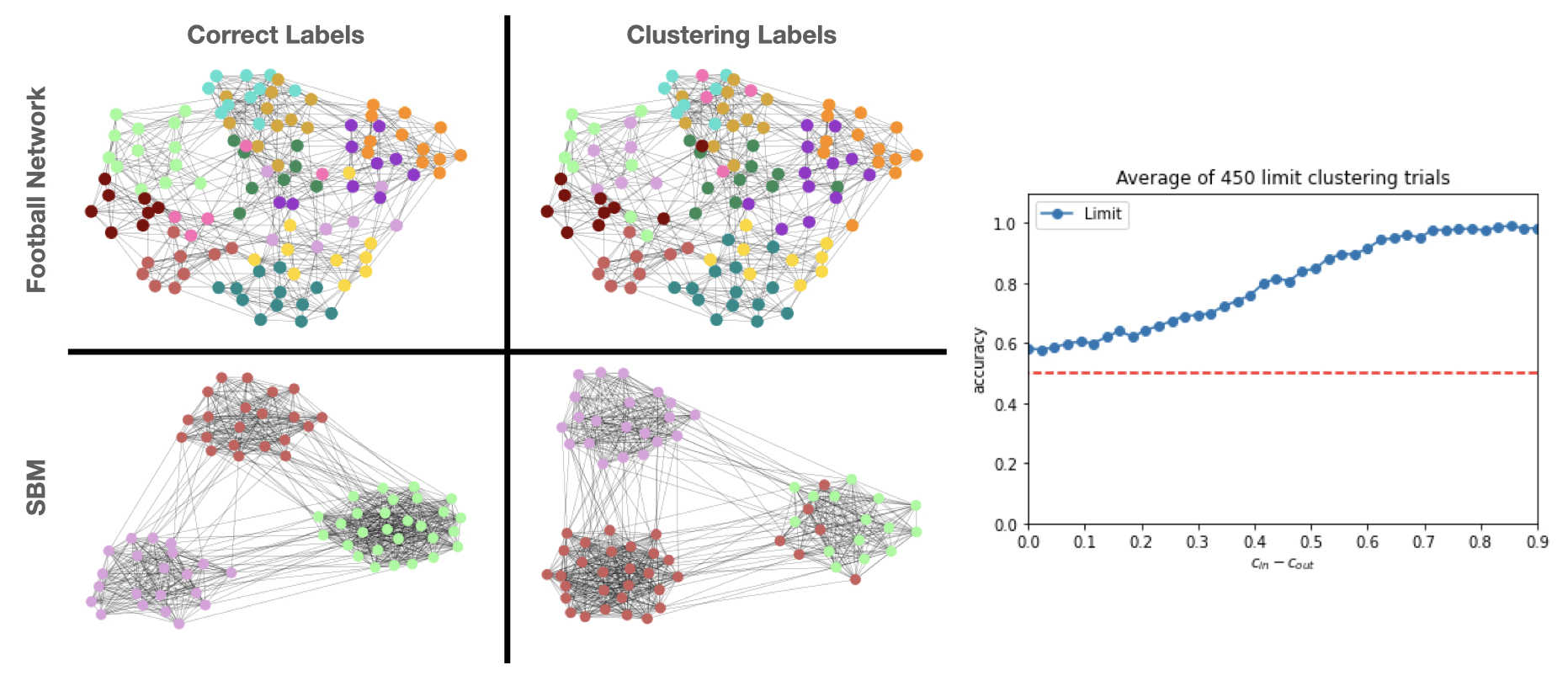
Figure 4: The top row is the football network and the bottom row is a random stochastic block network. The networks in the left column are the correctly labeled networks and the right are clustered networks. The plot on the right shows the algorithm accuracy as a function of the clustering strength in the network.

We now review the success of our algorithm on the Football network. This network of 114 nodes is a commonly used benchmark graph for new clustering algorithms. The goal is to be able to identify what conference each team corresponds to, thereby identifying 12 clusters. In Figure 4 the correct labels are shown, as well as the labels assigned by our algorithm. Our algorithm performed fairly well, with a normalized mutual information value of $0.8625$.

5 Conclusion

We have investigated the relationship between PageRank and its variants as well as various properties of its variants. Specifically, we have shown PageRank is equivalent to its variants in regular and bipartite biregular graphs. Using these variants, we defined a new centrality measure $\infty$-PageRank which can be used to approximate standard PageRank. Building off of the PageRank clustering work done by Chung and Tsiatas [10], we defined a new clustering algorithm based off of $\infty$-PageRank.

In addition to our findings, we have presented various conjectures which could prove vital for studying PageRank variants. As future work, we hope to investigate these conjectures further to create more efficient comparison between standard and non-backtracking PageRank.

References

- [1] David Aleja, Regino Criado, Alejandro J García del Amo, Ángel Pérez, and Miguel Romance. Non-backtracking pagerank: From the classic model to hashimoto matrices. Chaos, Solitons & Fractals, 126:283–291, 2019.
- [2] Noga Alon, Itai Benjamini, Eyal Lubetzky, and Sasha Sodin. Non-backtracking random walks mix faster. Communications in Contemporary Mathematics, 9(04):585–603, 2007.
- [3] Reid Andersen, Fan Chung, and Kevin Lang. Local graph partitioning using pagerank vectors. In 2006 47th Annual IEEE Symposium on Foundations of Computer Science (FOCS’06), pages 475–486. IEEE, 2006.
- [4] Francesca Arrigo, Desmond J Higham, and Vanni Noferini. Non-backtracking pagerank. Journal of Scientific Computing, 80(3):1419–1437, 2019.
- [5] Konstantin Avrachenkov and Dmitri Lebedev. Pagerank of scale-free growing networks. Internet Mathematics, 3(2):207–231, 2006.
- [6] Albert-László Barabási. Scale-free networks: a decade and beyond. science, 325(5939):412–413, 2009.
- [7] Albert-László Barabási and Eric Bonabeau. Scale-free networks. Scientific american, 288(5):60–69, 2003.
- [8] Regino Criado, Julio Flores, Esther García, Alejandro J García del Amo, Ángel Pérez, and Miguel Romance. On the -nonbacktracking centrality for complex networks: Existence and limit cases. Journal of Computational and Applied Mathematics, 350:35–45, 2019.
- [9] Alessandro Garavaglia, Remco van der Hofstad, and Nelly Litvak. Local weak convergence for pagerank. The Annals of Applied Probability, 30(1):40–79, 2020.
- [10] Fan Chung Graham and Alexander Tsiatas. Finding and visualizing graph clusters using pagerank optimization. In International Workshop on Algorithms and Models for the Web-Graph, pages 86–97. Springer, 2010.
- [11] Zoltan Gyongyi, Hector Garcia-Molina, and Jan Pedersen. Combating web spam with trustrank. In Proceedings of the 30th international conference on very large data bases (VLDB), 2004.
- [12] Julia Heidemann, Mathias Klier, and Florian Probst. Identifying key users in online social networks: A pagerank based approach. 2010.
- [13] Kenta Iwasaki and Kazuyuki Shudo. Estimating the clustering coefficient of a social network by a non-backtracking random walk. In 2018 IEEE International Conference on Big Data and Smart Computing (BigComp), pages 114–118. IEEE, 2018.
- [14] Mark Kempton. Non-backtracking random walks and a weighted ihara’s theorem. Open Journal of Discrete Mathematics, 6(4):207–226, 2016.
- [15] Keita Kitaura, Ryotaro Matsuo, and Hiroyuki Ohsaki. Random walk on a graph with vicinity avoidance. In 2022 International Conference on Information Networking (ICOIN), pages 232–237. IEEE, 2022.
- [16] Li Liu, Letian Sun, Shiping Chen, Ming Liu, and Jun Zhong. K-prscan: A clustering method based on pagerank. Neurocomputing, 175:65–80, 2016.
- [17] Rada Mihalcea, Paul Tarau, and Elizabeth Figa. Pagerank on semantic networks, with application to word sense disambiguation. In COLING 2004: Proceedings of the 20th International Conference on Computational Linguistics, pages 1126–1132, 2004.
- [18] Lawrence Page, Sergey Brin, Rajeev Motwani, and Terry Winograd. The pagerank citation ranking: Bringing order to the web. Technical report, Stanford InfoLab, 1999.
- [19] Jingzhi Pan, Fei Jiang, and Jin Xu. Influence maximization in social networks based on non-backtracking random walk. In 2016 IEEE First International Conference on Data Science in Cyberspace (DSC), pages 260–267. IEEE, 2016.
- [20] Shahram Payandeh and Eddie Chiu. Application of modified pagerank algorithm for anomaly detection in movements of older adults. International Journal of Telemedicine and Applications, 2019, 2019.
- [21] Dengwang Tang and Vijay G Subramanian. Balanced allocation on graphs with random walk based sampling. In 2018 56th Annual Allerton Conference on Communication, Control, and Computing (Allerton), pages 765–766. IEEE, 2018.
- [22] Leo Torres, Kevin S Chan, Hanghang Tong, and Tina Eliassi-Rad. Nonbacktracking eigenvalues under node removal: X-centrality and targeted immunization. SIAM Journal on Mathematics of Data Science, 3(2):656–675, 2021.
- [23] Ivan Voitalov, Pim van der Hoorn, Remco van der Hofstad, and Dmitri Krioukov. Scale-free networks well done. Physical Review Research, 1(3):033034, 2019.