Integrated Sensing and Communication: Joint Pilot and Transmission Design

Abstract

This paper studies a communication-centric integrated sensing and communication (ISAC) system, where a multi-antenna base station (BS) simultaneously performs downlink communication and target detection. A novel target detection and information transmission protocol is proposed, where the BS executes the channel estimation and beamforming successively and meanwhile jointly exploits the pilot sequences in the channel estimation stage and user information in the transmission stage to assist target detection. We investigate the joint design of the pilot matrix, training duration, and transmit beamforming to maximize the probability of target detection, subject to the minimum achievable rate required by the user. However, designing the optimal pilot matrix is rather challenging since there is no closed-form expression of the detection probability with respect to the pilot matrix. To tackle this difficulty, we resort to designing the pilot matrix based on the information-theoretic criterion to maximize the mutual information (MI) between the received observations and BS-target channel coefficients for target detection. We first derive the optimal pilot matrix for both channel estimation and target detection, and then propose a unified pilot matrix structure to balance minimizing the channel estimation error (MSE) and maximizing MI. Based on the proposed structure, a low-complexity successive refinement algorithm is proposed. In addition, we rigorously analyze the impact of pilot length and pilot matrix on two fundamental tradeoffs, namely MSE-MI and Rate-MI. Simulation results demonstrate that the proposed pilot matrix structure can well balance the MSE-MI and the Rate-MI tradeoffs, and show the significant region improvement of our proposed design as compared to other benchmark schemes. Furthermore, it is unveiled that as the communication channel is more spatially correlated, the Rate-MI region can be further enlarged.

I Introduction

Future emerging applications such as Internet of Things (IoT) smart cities will pose new requirements on future wireless communication networks [1, 2, 3], which not only require high-data-rate and low-latency communication services but also additional high precision and high-resolution sensing functions. As shown by Statista organization, the number of IoT devices is predicated to grow from $13.1$ billion in 2022 to more than $29.4$ billion in 2030 [4]. To support such massive amount of smart IoT devices, the integrated sensing and communication (ISAC) technology is recently proposed, where the base station (BS) integrates the sensing and communication functions into a common platform and can operate two functions in the same frequency band [5, 6, 7, 8, 9, 10].

Different from the coexistence system where the radar and communication hardware modules are physically separated, they are physically integrated into the ISAC system. Thus, several appealing advantages are introduced as follows [11]. 1) Ease of integration: The majority of transmitter/receiver modules can be shared by radar and communication systems, which makes it easy to implement from hardware perspectives; 2) Integration gain: The components or resources in the ISAC system can be coupled to achieve more efficient resource utilization such that the signal overhead can be reduced and the spectral and energy efficiency can be improved; 3) Coordination gain: One can flexibly balance the dual-functional performance via mutual assistance such as jointly designing the waveforms. As such, a large number of works have paid attention to it in the literature, which can be classified into three paradigm directions of research, namely radar-centric design [12, 13, 14], communication-centric design [15, 16, 17], and joint design and optimization [18, 19, 20, 21, 22], on the ISAC system based on the different integration approaches. For example, in [12], the authors considered the radar system as the primary function and embedded communication signals into the radar waveform by controlling its amplitude and phase of the radar spatial side-lobe to convey information. In [15], the authors considered the existing communication transmitter hardware and applied the orthogonal frequency-division multiplexing (OFDM) communication signals to realize the radar sensing functionality. The authors in [19] proposed a new hardware architecture which is able to jointly design communication and radar waveforms to realize both communication and sensing functionalities.

However, it is worth pointing out that none of the above works focused on the ISAC system design considering both the downlink training and information transmission phases. It still remains unknown how the pilot matrix, the training duration, and the transmit beamformer impact communication and sensing. First, since the second-order statistic of the channel state information (CSI) for the communication user channel and the target channel is in general different, the optimal pilot matrix for channel estimation may not be optimal for target sensing, and vice versa. Second, if a longer training duration is used for improving the accuracy of channel estimation, less time is left for data transmission, which gives rise to a fundamental tradeoff between channel estimation accuracy and data transmission. Furthermore, the time allocated for channel estimation and information transmission will also impact the target sensing since the pilot signals and the information signals are not the same. To be specific, the pilot matrix is deterministic and remains unchanged over a whole channel coherence while the information signals are random and vary over different time slots. Third, the optimal transmit beamformer for information transmission and target sensing is different since the narrow beam is expected to focus all the energy on the communication user, while a flat beam is desired for target sensing since the target location is unknown. Therefore, a unified resource allocation, i.e., space-time code/pilot matrix, training duration, and the transmit beamformer, on the ISAC system should be thoroughly studied, which thus motivates this work. We note that [23] studied the optimal space-time code design for radar detection, whereas only the radar system was considered and its impact on the communication system still remains unknown. In addition, the authors in [24] unveiled the impact of pilot training duration on the communication system performance while its impact on the radar system was not studied. However, their insights will not be true in the ISAC system and their proposed transceiver designs are also no longer applicable due to the joint resource allocation.

Figure 1: A communication-centric ISAC system.

As shown in Fig. 1, we consider a communication-centric frequency-division duplexing (FDD) ISAC system with one BS, one potential target, and one communication user, where the BS simultaneously performs downlink communication and target detection. This paper attempts to study the performance tradeoff between communication and sensing based on the communication-centric ISAC systems where the BS leverages the communication waveforms to perform sensing. We study the resource allocation, namely pilot training duration, transmit beamformer, and space-time code/pilot matrix, on the ISAC system to maximize the target detection probability while guaranteeing the communication system performance. Particularly, we unveil two tradeoffs, namely channel estimation error (MSE)-mutual information (MI) and Rate-MI, on the ISAC. It is worth mentioning that our work differs significantly from [25] in four aspects. First, [25] studies a time-division duplexing (TDD) ISAC system where the BS sends downlink pilot signals for target detection and the user sends uplink pilot signals to the BS for channel estimation, while our work studies an FDD ISAC system where the BS sends downlink pilot signals for target detection and the user performs channel estimation. Second, the objective of [25] is to enhance sensing performance by exploiting joint burst sparsity and pilot design, while our work is to study the performance tradeoff between communication and sensing under the pilot matrix, the training duration, and the transmit beamformer. Third, the proposed algorithm in [25] is not applicable to our considered optimization problem, we propose an efficient algorithm to cater to the formulated optimization problem. Fourth, [25] does not consider the communication performance, while our work considers the impact of pilot duration and pilot signals on the ISAC system. The contributions of his paper are summarized as follows:

• We propose a novel target detection and information transmission protocol, where both the channel estimation stage and information transmission stage are used to target detection. The closed-form formulas for the false alarm and the detection probability based on the generalized likelihood ratio test (GLRT) are derived. Then, a target detection probability maximization optimization problem is formulated by jointly optimizing pilot training duration, transmit beamformer, and space-time code/pilot matrix, subject to the minimum achievable rate required by the communication user.

• To minimize the channel estimation error, we find that the optimal pilot matrix is nonunitary with different power allocation. The analysis shows that with a fixed power budget, a larger training duration leads to a smaller MSE, while the MSE will not be further reduced as the training duration is larger than the rank of the channel covariance matrix. In contrast, to maximize the target detection probability based on the MI merit, we find that the optimal pilot matrix is unitary with equal power allocation. We prove that with a fixed power budget, a larger training duration leads to a larger MI, while the MI will not be further increased as the training duration is larger than the number of transmit antennas. Based on these observations, a novel pilot matrix structure is proposed that balances the tradeoff between the MSE and the MI. Then, we solve the resulting optimization problem based on the block coordinate descent (BCD) approach, where the beamformer and pilot matrix are alternately optimized.

• Simulation results show that the proposed design is capable of substantially improving the target detection probability, Rate-MI region, and MSE-MI region compared to the benchmark schemes. In addition, several interesting insights are unveiled. First, the proposed pilot structure can well balance the communication performance and the sensing performance, and show the superiority of the proposed pilot structure over the discrete Fourier transform (DFT) matrix and Gaussian-based matrix. Second, the optimal training duration for maximizing the Rate-MI region is not equal to the rank of the channel covariance matrix. Third, the Rate-MI region can be further enlarged for a more spatially correlated communication channel.

The rest of this paper is organized as follows. Section II introduces the system model and the problem formulation for the considered communication-centric ISAC. In Section III, the novel pilot matrix structure is proposed and a BCD-based algorithm is further introduced to solve the resulting optimization problem. Numerical results are provided in Section IV and the paper is concluded in Section V.

Notations: Boldface upper-case and lower-case letters denote matrices and vectors, respectively. ${{\bf{1}}_{L}}$ represents a vector of all ones with the length of $L$. ${\mathbb{C}}^{d_{1}\times d_{2}}$ stands for the set of complex $d_{1}\times d_{2}$ matrices. For a complex-valued vector $\bf x$, ${\left\|{\bf x}\right\|}$ represents the Euclidean norm of $\bf x$, and ${\rm diag}(\bf x)$ denotes a diagonal matrix whose main diagonal elements are extracted from vector $\bf x$. ${\left(\cdot\right)^{T}},{\left(\cdot\right)^{*}}$, ${\left(\cdot\right)^{H}}$, and ${\left(\cdot\right)^{{\dagger}}}$stand for the transpose operator, conjugate operator, conjugate transpose, and pseudo inverse operator, respectively. ${\left\|{\bf{X}}\right\|_{F}}$ represents the Frobenius norm of ${\bf{X}}$, ${\bf{X}}\succeq{\bf{0}}$ indicates that matrix $\bf X$ is positive semi-definite, and ${\bf{X}}\left({1:L}\right)$ stands for the matrix containing the first $L$ columns of ${\bf{X}}$. A circularly symmetric complex Gaussian (CSCG) vector $\bf x$ with mean $\bm{\mu}$ and covariance matrix ${\sigma^{2}}{\bf{I}}$ is denoted by ${\bf x}\sim{\cal CN}\left({{{\bm{\mu}}},{{\sigma^{2}{\bf{I}}}}}\right)$. ${\mathbb{Z}}^{+}$ represents the positive integer notation. $\otimes$ denotes the Kronecker product operator and ${\cal O}\left(\cdot\right)$ is the big-O computational complexity notation.

II System Model and Problem Formulation

Consider a narrow-band ISAC system consisting of one BS, one single-antenna user, and one potential target, as shown in Fig. 1. The BS is equipped with $N_{t}+N_{r}$ antennas, of which $N_{t}$ transmit antennas are used for simultaneously serving communication users and sensing radar targets in the same frequency band, while $N_{r}$ receive antennas are dedicated to receiving the echo signals reflected by the target. We consider a quasi-static flat-fading channel in which the CSI remains unchanged in a channel coherence frame, but may change in the subsequent frames. Note that the frames of interest have the same channel fading statistical distribution so that the same pilot training sequences and the training duration can be applied for all the frames. Without loss of generality, we denote the channel coherence duration of each frame by $T_{c}$ (in symbols).

Figure 2: Target detection and information transmission protocol.

We consider an FDD system where the BS sends the downlink pilot sequences to the user for channel estimation, which then feeds back the CSI to the BS. The target detection and information transmission protocol is shown in Fig. 2, in which one channel coherence time is divided into two stages, namely stage I and stage II. In stage I, the BS transmits $L$ pilot symbols for the estimation and meanwhile these pilot symbols are used for target detection. In stage II, the BS transmits to the user $T_{c}-L$ data symbols, which are also used for target detection. Under this protocol, the target detection is fully utilized during one channel coherence time. For convenience, we denote the sets of BS transmit antennas, BS receive antennas, pilot symbols, and channel coherence interval as ${\cal N}_{t}$, ${\cal N}_{r}$, $\cal L$, and ${\cal T}_{c}$, respectively. In this paper, our analysis is based on the spatially correlated Rician channel model for the communication channel and the uncorrelated channel model for the radar channel. The analysis of the other channels such as the multipath channel model is interesting but requires non-trivial efforts and we would like to leave them as our future work.

II-A Communication-Centric Target Detection

In stage I, the signal received at the $i$th BS receive antenna during the $l$th symbol is given by

$${y_{r,i}}\left[l\right]=\sum\limits_{j=1}^{{N_{t}}}{{g_{i,j}}{x_{c,j}}\left[l\right]}+{n_{r,i}}\left[l\right],i\in{\cal N}_{r},l\in{\cal L},$$ (1)

where ${x_{c,j}}\left[l\right]$ denotes the $l$th pilot symbol transmitted by the $j$th BS transmit antenna, $g_{i,j}$ stands for the round-trip channel coefficient between the $j$th BS transmit antenna and the $i$th BS receive antenna, and ${n_{r,i}}\left[l\right]\sim{\cal CN}\left({0,\sigma_{r}^{2}}\right)$ stands for the additive white Gaussian noise. Note that in the sequel, we assume that round-trip channel coefficients $g_{i,j}$’s are independent by assuming that the transmit antennas and receive antennas at the BS are sufficiently spaced so that the angle diversity can be explored. In addition, we consider a Swerling-I target model, where the channel coefficient follows identically distributed CSCG with mean $0$ and variance ${\delta_{g}^{2}}$, i.e., ${g_{i,j}}\sim{\cal CN}\left({0,\delta_{g}^{2}}\right)$ [23].

Upon collecting $L$ symbols at the $i$th BS receive antenna and defining ${{\bf{y}}_{r,i}^{\rm I}}={\left[{{y_{r,i}}\left[1\right],\ldots,{y_{r,i}}\left[L\right]}\right]^{T}}$, we can rewrite it as a vector form given by

$${{\bf{y}}_{r,i}^{\rm I}}={{\bf{X}}_{c}}{{\bf{g}}_{i}}+{{\bf{n}}_{r,i}^{\rm I}},i\in{\cal N}_{r},$$ (2)

where ${{\bf{X}}_{c}}=\left[{\begin{array}[]{*{20}{c}}{{x_{c,1}}\left[1\right]}&\cdots&{{x_{c,{N_{t}}}}\left[1\right]}\\ \vdots&\ddots&\vdots\\ {{x_{c,1}}\left[L\right]}&\cdots&{{x_{c,{N_{t}}}}\left[L\right]}\end{array}}\right]$, ${{\bf{g}}_{i}}={\left[{{g_{i,1}},\ldots,{g_{i,{N_{t}}}}}\right]^{T}}$, and ${{\bf{n}}_{r,i}^{\rm I}}={\left[{{n_{r,i}}\left[1\right],\ldots,{n_{r,i}}\left[L\right]}\right]^{T}}$.

Similar to stage I, the pilot symbols in stage II are replaced by the data symbols for transmission. As such, we can write the signal received at the $i$th BS receive antenna after collecting $T_{c}-L$ data symbols in stage II as

$${\bf{y}}_{r,i}^{{\rm{II}}} ={\rm{diag}}\left({{x_{t}}\left[{L{\rm{+}}1}\right],\ldots,{x_{t}}\left[{{T_{c}}}\right]}\right){{\bf{1}}_{{T_{c}}-L}}{{\bf{w}}^{T}}{{\bf{g}}_{i}}+{\bf{n}}_{r,i}^{{\rm{II}}}$$

$$={{\bf{X}}_{t}}{{\bf{g}}_{i}}+{\bf{n}}_{r,i}^{{\rm{II}}},i\in{\cal N}_{r},$$ (3)

where ${{\bf{X}}_{t}}={\rm{diag}}\left({{x_{t}}\left[{L{\rm{+}}1}\right],\ldots,{x_{t}}\left[{{T_{c}}}\right]}\right){{\bf{1}}_{{T_{c}}-L}}{\bf{w}}^{T}$, ${{x_{t}}\left[j\right]}$ denotes the $j$th data symbol, ${\bf{w}}\in{{\mathbb{C}}^{{N_{t}}\times 1}}$ stands for the transmit beamformer, and ${\bf{n}}_{r,i}^{{\rm{II}}}$ denotes the received white Gaussian noise satisfying ${\bf{n}}_{r,i}^{{\rm{II}}}\sim{\cal CN}\left({{{\bf{0}}_{\left({{T_{c}}-L}\right)\times 1}},\sigma_{r}^{2}{{\bf{I}}_{{T_{c}}-L}}}\right)$.

Based on the presence (hypothesis ${{\cal H}_{1}}$) or absence (hypothesis ${{\cal H}_{0}}$) of the target, a binary hypothesis test over one channel coherence time is formulated as

$${{\cal H}_{0}}:\;\;\;{\mkern 1.0mu}\left\{{\begin{array}[]{*{20}{l}}{{\bf{y}}_{r,i}^{\rm{I}}={\bf{n}}_{r,i}^{\rm{I}},i\in{\cal N}_{r},\;\;\;{\mkern 1.0mu}{\rm{stage~{}I}},}\\ {{\bf{y}}_{r,i}^{{\rm{II}}}={\bf{n}}_{r,i}^{{\rm{II}}},i\in{\cal N}_{r},\;\;\;{\mkern 1.0mu}{\rm{stage~{}II}}.}\end{array}}\right.$$ (6)

$${{\cal H}_{1}}:\;\;\;\left\{{\begin{array}[]{*{20}{l}}{{\bf{y}}_{r,i}^{\rm{I}}={{\bf{X}}_{c}}{{\bf{g}}_{i}}+{\bf{n}}_{r,i}^{\rm{I}},i\in{\cal N}_{r},\;\;\;{\mkern 1.0mu}{\rm{stage~{}I}},}\\ {{\bf{y}}_{r,i}^{{\rm{II}}}={\bf{X}}_{t}{{\bf{g}}_{i}}+{\bf{n}}_{r,i}^{{\rm{II}}},i\in{\cal N}_{r},\;\;\;{\mkern 1.0mu}{\rm{stage~{}II}}.}\end{array}}\right.$$ (9)

It can be readily checked that the hypothesis testing problem in (9) belongs to a model change detection problem, where the mean value will jump with the change of time (see stage I and stage II in ${\cal H}_{1}$). Define ${{\bf{y}}_{r,i}}={\left[{{\bf{y}}_{r,i}^{{\rm{I,}}T}{\kern 1.0pt}{\kern 1.0pt}{\kern 1.0pt}{\kern 1.0pt}{\kern 1.0pt}{\kern 1.0pt}{\bf{y}}_{r,i}^{{\rm{II,}}T}}\right]^{T}}$ and ${{\bf{n}}_{r,i}}={\left[{{\bf{n}}_{r,i}^{{\rm{I,}}T}{\kern 1.0pt}{\kern 1.0pt}{\kern 1.0pt}{\kern 1.0pt}{\kern 1.0pt}{\kern 1.0pt}{\bf{n}}_{r,i}^{{\rm{II,}}T}}\right]^{T}}$. Then, we can rewrite (9) in a more compact form given by

$${{\cal H}_{0}}:\;\;\;{\mkern 1.0mu}{{\bf{y}}_{r,i}}={{\bf{n}}_{r,i}},i\in{\cal N}_{r},$$

$${{\cal H}_{1}}:\;\;\;{{\bf{y}}_{r,i}}={\bf{X}}{{\bf{g}}_{i}}+{{\bf{n}}_{r,i}},i\in{\cal N}_{r},$$ (10)

where ${\bf{X}}={\left[{{\bf{X}}_{c}^{T}{\kern 1.0pt}{\kern 1.0pt}{\kern 1.0pt}{\bf{X}}_{t}^{T}}\right]^{T}}$.

Since the prior information about ${\bf g}_{i}$’s is unknown, the traditional Neyman–Pearson criterion cannot be applied. Instead, the generalized likelihood ratio test (GLRT) is adopted, which replaces the unknown parameters with their maximum likelihood (ML) estimates under each hypothesis. Specifically, under the hypothesis test in (10), the GLRT decides ${\cal H}_{1}$ or ${\cal H}_{0}$ as follows:

$$\frac{{\mathop{\max}\limits_{\left\{{{{\bf{g}}_{i}}}\right\}}f\left({{{\bf{y}}_{r,1}}\ldots,{{\bf{y}}_{r,{N_{r}}}};{{\bf{g}}_{1}},\ldots,{{\bf{g}}_{{N_{r}}}}|{{\cal H}_{1}}}\right)}}{{f\left({{{\bf{y}}_{r,1}}\ldots,{{\bf{y}}_{r,{N_{r}}}}|{{\cal H}_{0}}}\right)}}\mathop{\gtrless}_{{\cal H}_{0}}^{{\cal H}_{1}}{\Gamma_{{{\rm th}}}},$$ (11)

where ${\Gamma_{{{\rm th}}}}$ denotes the decision threshold, $f\left({{{\bf{y}}_{r,1}}\ldots,{{\bf{y}}_{r,{N_{r}}}};{{\bf{g}}_{1}},\ldots,{{\bf{g}}_{{N_{r}}}}|{{\cal H}_{1}}}\right)$ and $f\left({{{\bf{y}}_{r,1}}\ldots,{{\bf{y}}_{r,{N_{r}}}}|{{\cal H}_{0}}}\right)$ denote the probability density functions (PDFs) of the data under hypotheses ${\cal H}_{1}$ and ${\cal H}_{0}$ from $N_{r}$ receive antennas, which are respectively given by

$$f\left({{{\bf{y}}_{r,1}}\ldots,{{\bf{y}}_{r,{N_{r}}}}|{{\cal H}_{0}}}\right)=$$

$$\qquad\qquad\frac{1}{{{\pi^{{T_{c}}{N_{r}}}}\sigma_{r}^{2{T_{c}}{N_{r}}}}}\exp\left({-\frac{1}{{\sigma_{r}^{2}}}\sum\limits_{i=1}^{{N_{r}}}{{{\left\|{{{\bf{y}}_{r,i}}}\right\|}^{2}}}}\right),$$ (12)

$$f\left({{{\bf{y}}_{r,1}}\ldots,{{\bf{y}}_{r,{N_{r}}}};{{\bf{g}}_{1}},\ldots,{{\bf{g}}_{{N_{r}}}}|{{\cal H}_{1}}}\right)=$$

$$\qquad\frac{1}{{{\pi^{{T_{c}}{N_{r}}}}\sigma_{r}^{2{T_{c}}{N_{r}}}}}\exp\left({-\frac{1}{{\sigma_{r}^{2}}}\sum\limits_{i=1}^{{N_{r}}}{{{\left\|{{{\bf{y}}_{r,i}}-{\bf{X}}{{\bf{g}}_{i}}}\right\|}^{2}}}}\right).$$ (13)

Substituting (12) and (13) into (11), we can further simplify (11) to

$$\frac{1}{{\sigma_{r}^{2}}}\left(\sum\limits_{i=1}^{{N_{r}}}{{{\left\|{{{\bf{y}}_{r,i}}}\right\|}^{2}}}-\mathop{\min}\limits_{\left\{{{{\bf{g}}_{i}}}\right\}}\sum\limits_{i=1}^{{N_{r}}}{{{\left\|{{{\bf{y}}_{r,i}}-{\bf{X}}{{\bf{g}}_{i}}}\right\|}^{2}}}\right)\mathop{\gtrless}_{{\cal H}_{0}}^{{\cal H}_{1}}{{\hat{\Gamma}}_{{{\rm th}}}},$$ (14)

where ${{\hat{\Gamma}}_{{{\rm th}}}}=\ln{\Gamma_{{{\rm th}}}}$.

Let ${{{\bf{\hat{g}}}}_{i}}$ be the ML estimate of ${{{\bf{g}}}_{i}}$ under hypotheses ${\cal H}_{1}$, $i\in{\cal N}_{r}$. Taking the first-order derivative of ${{{\left\|{{{\bf{y}}_{r,i}}-{\bf{X}}{{\bf{g}}_{i}}}\right\|}^{2}}}$ with respect to (w.r.t.) ${{{\bf{g}}_{i}}}$ and setting it to zero, we have

$${{{\bf{\hat{g}}}}_{i}}={\left({{{\bf{X}}^{H}}{\bf{X}}}\right)^{{\dagger}}}{{\bf{X}}^{H}}{{\bf{y}}_{r,i}},i\in{\cal N}_{r}.$$ (15)

Then, substituting (15) into (14), we have

$$\frac{1}{{\sigma_{r}^{2}}}\left(\sum\limits_{i=1}^{{N_{r}}}{{\bf{y}}_{r,i}^{H}}{\bf{X}}{\left({{{\bf{X}}^{H}}{\bf{X}}}\right)^{{\dagger}}}{{\bf{X}}^{H}}{{\bf{y}}_{r,i}}\right)\mathop{\gtrless}_{{\cal H}_{0}}^{{\cal H}_{1}}{{\hat{\Gamma}}_{{{\rm th}}}}.$$ (16)

In this paper, we assume that the pilot-based matrix ${\bf{X}}_{c}$ is a full-rank matrix to achieve the maximum spatial multiplexing gain. In addition, based on the fact that the pilot symbols and data symbols are independent in general, we have the following lemma.

Lemma 1: If ${\bf{X}}_{c}$ is a full-rank matrix and ${{\bf{X}}_{t}}\neq{\bf{0}}$, i.e., ${\rm{rank}}\left({{{\bf{X}}_{c}}}\right)=\min\left({L,{N_{t}}}\right)$, the rank of $\bf X$ is given by ${\rm{rank}}\left({\bf{X}}\right)=\min\left({L+1,{N_{t}}}\right)$.

Proof: This can be directly verified from the definition and is thus omitted here.  

Lemma 2: ${\rm{rank}}\left({{\bf{X}}{{\left({{{\bf{X}}^{H}}{\bf{X}}}\right)}^{\dagger}}{{\bf{X}}^{H}}}\right)={\rm{rank}}\left({\bf{X}}\right)$.

Proof: Please refer to Appendix A.  

Lemma 3: ${{\bf{X}}{{\left({{{\bf{X}}^{H}}{\bf{X}}}\right)}^{\dagger}}{{\bf{X}}^{H}}}$ is idempotent and has $L+1$ eigenvalues of one and $T_{c}-L-1$ eigenvalues of zero when $L\leq N_{t}-1$, while it has $N_{t}$ eigenvalues of one and $T_{c}-N_{t}$ eigenvalues of zero when $L>N_{t}-1$.

Proof: Please refer to Appendix B.  

II-A1 Probability of False Alarm

Under hypothesis ${\cal H}_{0}$, the received signal at the $i$th receiver given in (10) satisfies ${{\bf{y}}_{r,i}}\sim{\cal CN}\left({{\bf{0}},\sigma_{r}^{2}{{\bf{I}}_{{T_{c}}}}}\right)$. Let ${{\bf{z}}_{r,i}}={\bf{U}}^{H}{{\bf{y}}_{r,i}}$ and recall that ${\bf{X}}{\left({{{\bf{X}}^{H}}{\bf{X}}}\right)^{\dagger}}{{\bf{X}}^{H}}={{\bf{U}}_{\bf{x}}}{\bf{U}}_{\bf{x}}^{H}$ (see in Appendix B), it can readily follow that ${{\bf{z}}_{r,i}}\sim{\cal CN}\left({0,\sigma_{r}^{2}{{\bf{I}}_{{\min\left({L+1,{N_{t}}}\right)}}}}\right)$ based on the fact that an orthogonal transformation will not change the distribution of ${{\bf{y}}_{r,i}}$. Then, the left-hand side of (16) can be rewritten as

$$\frac{1}{{\sigma_{r}^{2}}}\left({\sum\limits_{i=1}^{{N_{r}}}{{\bf{y}}_{r,i}^{H}}{\bf{X}}{{\left({{{\bf{X}}^{H}}{\bf{X}}}\right)}^{\dagger}}{{\bf{X}}^{H}}{{\bf{y}}_{r,i}}}\right)=\sum\limits_{i=1}^{{N_{r}}}{{{\left({\frac{{{{\bf{z}}_{r,i}}}}{{{\sigma_{r}}}}}\right)}^{H}}\frac{{{{\bf{z}}_{r,i}}}}{{{\sigma_{r}}}}},$$ (17)

with ${{\bf{z}}_{r,i}}/{\sigma_{r}}\sim{\cal CN}\left({{\bf 0},{{\bf{I}}_{{\min\left({L+1,{N_{t}}}\right)}}}}\right)$. It can be readily verified that (17) follows the central chi-squared distribution since it has a sum of the squares of $2{N_{r}}\min\left({L+1,{N_{t}}}\right)$ independently real Gaussian random variables, each of which satisfies zero mean and variance $1/2$. As such, the PDF of (17) is given by [28]

$${p_{Z}}\left({z|{{\cal H}_{0}}}\right)=\frac{{{z^{\frac{1}{2}\min\left({L+1,{N_{t}}}\right)-1}}}}{{\int_{0}^{+\infty}{{t^{\frac{1}{2}\min\left({L+1,{N_{t}}}\right)-1}}}{e^{-t}}dt}}{e^{-z}},z\geq 0.$$ (18)

Then, the probability of false alarm can be derived as [28]

$${P_{{\rm{fa}}}} =\int_{{{\hat{\Gamma}}_{{\rm{th}}}}}^{+\infty}{{p_{Z}}\left({z|{{\cal H}_{0}}}\right)dz}$$

$$={e^{-{{\hat{\Gamma}}_{{\rm{th}}}}}}\sum\limits_{k=0}^{{N_{r}}\min\left({L+1,{N_{t}}}\right)-1}{\frac{1}{{k!}}}\hat{\Gamma}_{{\rm{th}}}^{k}.$$ (19)

II-A2 Probability of Detection

Under hypothesis ${\cal H}_{1}$, the received signal at the $i$th receiver given in (10) satisfies ${{\bf{y}}_{r,i}}\sim{\cal CN}\left({{\bf{X}}{{\bf{g}}_{i}},\sigma_{r}^{2}{{\bf{I}}_{{T_{c}}}}}\right)$. Similar to the hypothesis ${\cal H}_{0}$ case, define ${{\bf{z}}_{r,i}}={\bf{U}}^{H}{{\bf{y}}_{r,i}}$, it follows that ${{\bf{z}}_{r,i}}\sim{\cal CN}\left({{\bf{U}}_{\bf{x}}^{H}{\bf{X}}{{\bf{g}}_{i}},\sigma_{r}^{2}{{\bf{I}}_{\min\left({L+1,{N_{t}}}\right)}}}\right)$. This indicates that each entry of ${{\bf{z}}_{r,i}}$ follows the Gaussian distribution and has the same variance but with different means. As such, $\frac{1}{{\sigma_{r}^{2}}}\left({\sum\limits_{i=1}^{{N_{r}}}{{\bf{y}}_{r,i}^{H}}{\bf{X}}{{\left({{{\bf{X}}^{H}}{\bf{X}}}\right)}^{\dagger}}{{\bf{X}}^{H}}{{\bf{y}}_{r,i}}}\right)$ follows the non-central chi-squared distribution with the PDF given by

$${p_{Z}}\left({z|{{\cal H}_{1}}}\right) ={\left({\frac{z}{{{s^{2}}}}}\right)^{\left({{N_{r}}\min\left({L+1,{N_{t}}}\right)-1}\right)/2}}{e^{-\left({{s^{2}}+z}\right)}}$$

$$\times{I_{{N_{r}}\min\left({L+1,{N_{t}}}\right)-1}}\left({2\sqrt{z}s}\right),$$ (20)

where ${I_{\alpha}}\left({2\sqrt{z}s}\right)$ represents the Bessel function of the first kind of order $\alpha$ and the noncentrality parameter ${s^{2}}$ is given by

$${s^{2}} =\sum\limits_{i=1}^{{N_{r}}}{{{\left\|{{\bf{U}}_{\bf{x}}^{H}{\bf{X}}{{\bf{g}}_{i}}}\right\|}^{2}}/\sigma_{r}^{2}}$$

$$\overset{(a)}{=}\sum\limits_{i=1}^{{N_{r}}}{\left\|{{\bf{U}}_{\bf{x}}^{H}{{\bf{U}}_{\bf{x}}}{{\bf{\Sigma}}_{\bf{x}}}{\bf{V}}_{\bf{x}}^{H}{{\bf{g}}_{i}}}\right\|_{F}^{2}/\sigma_{r}^{2}}$$

$$=\sum\limits_{i=1}^{{N_{r}}}{{\rm{tr}}\left({{{\bf{\Sigma}}_{\bf{x}}}{\bf{V}}_{\bf{x}}^{H}{{\bf{g}}_{i}}{\bf{g}}_{i}^{H}{{\bf{V}}_{\bf{x}}}{{\bf{\Sigma}}_{\bf{x}}}}\right)/\sigma_{r}^{2}}$$

$$=\sum\limits_{i=1}^{{N_{r}}}{{\rm{tr}}\left({{\bf{X}}{{\bf{g}}_{i}}{\bf{g}}_{i}^{H}{{\bf{X}}^{H}}}\right)/\sigma_{r}^{2}}=\left\|{\frac{1}{{{\sigma_{r}}}}{\bf{XG}}}\right\|_{F}^{2},$$ (21)

where equality (a) holds due to ${\bf{X}}={{\bf{U}}_{\bf{x}}}{{\bf{\Sigma}}_{\bf{x}}}{\bf{V}}_{\bf{x}}^{H}$ defined in Appendix A.

As a consequence, the probability of detection can be derived as [28]

$${P_{d}} =\int_{{{\hat{\Gamma}}_{{\rm{th}}}}}^{+\infty}{{p_{Z}}\left({z|{{\cal H}_{1}}}\right)dz}$$

$$={Q_{{N_{r}}\min\left({L+1,{N_{t}}}\right)}}\left({\sqrt{2}s,\sqrt{2{{\hat{\Gamma}}_{{\rm{th}}}}}}\right)$$

$$={Q_{{N_{r}}\min\left({L+1,{N_{t}}}\right)}}\left({\sqrt{2}{{\left\|{\frac{1}{{{\sigma_{r}}}}{\bf{XG}}}\right\|}_{F}},\sqrt{2{{\hat{\Gamma}}_{{\rm{th}}}}}}\right),$$ (22)

where ${Q_{m}}\left({:,:}\right)$ is the generalized Marcum $Q$ function of order $m$ and ${\bf{G}}=\left({{{\bf{g}}_{1}},\ldots,{{\bf{g}}_{{N_{r}}}}}\right)$.

II-B Channel Estimation and Information Transmission

II-B1 Channel Estimation

Denote by ${\bf{h}}\in{{\mathbb{C}}^{{N_{t}}\times 1}}$ the communication channel between the BS and the user. To estimate $\bf h$, $L$ pilot sequences, i.e., ${\bf X}_{c}$ are applied. Then, the signal received during stage I can be compactly written as

$${{\bf{y}}_{p}}={{\bf{X}}_{c}}{\bf{h}}+{{\bf{n}}_{p}},$$ (23)

where ${{\bf{n}}_{p}}\sim{\cal CN}\left({{\bf 0},\sigma_{p}^{2}{\bf I}_{L\times 1}}\right)$ represents the white Gaussian noise received by the user.

Based on the signals received in (23), the minimum mean square error (MMSE) estimator is applied for estimating $\bf h$. Specifically, the MMSE estimator is given by

$$\!\!\!J\left({\bf{F}}\right)=\mathop{\min}\limits_{\bf{F}}{\mathbb{E}}\left\{{\left\|{{\bf{h}}-{\bf{\hat{h}}}}\right\|^{2}}\right\}=\mathop{\min}\limits_{\bf{F}}{\mathbb{E}}\left\{{\left\|{{\bf{h}}-{\bf{F}}{{\bf{y}}_{p}}}\right\|^{2}}\right\},$$ (24)

where ${\bf{\hat{h}}}$ denotes the estimated channel and ${\bf{F}}\in{{\mathbb{C}}^{{N_{t}}\times L}}$ is a matrix to be optimized for minimizing the mean square error (MSE) of the channel estimation. By taking the first-order derivative of ${{{\left\|{{\bf{h}}-{\bf{F}}{{\bf{y}}_{p}}}\right\|}^{2}}}$ w.r.t. ${\bf{F}}$ and setting it to zero, the optimal ${\bf{F}}\in{{\mathbb{C}}^{{N_{t}}\times L}}$ can be obtained as

$${{\bf{F}}^{{\rm{opt}}}}={{\bf{R}}_{\bf{h}}}{\bf{X}}_{c}^{H}{\left({{{\bf{X}}_{c}}{{\bf{R}}_{\bf{h}}}{\bf{X}}_{c}^{H}+\sigma_{p}^{2}{{\bf{I}}_{L}}}\right)^{-1}},$$ (25)

where ${{\bf{R}}_{\bf{h}}}={\mathbb{E}}\left\{{{\bf{h}}{{\bf{h}}^{H}}}\right\}$. Then, the estimation of $\bf h$ is given by

$${\bf{\hat{h}}}={{\bf{F}}^{{\rm{opt}}}}{{\bf{y}}_{p}}={{\bf{R}}_{\bf{h}}}{\bf{X}}_{c}^{H}{\left({{{\bf{X}}_{c}}{{\bf{R}}_{\bf{h}}}{\bf{X}}_{c}^{H}+\sigma_{p}^{2}{{\bf{I}}_{L}}}\right)^{-1}}{{\bf{y}}_{p}},$$ (26)

with covariance matrix of ${\bf{\hat{h}}}$ given by

$${{\bf{R}}_{{\bf{\hat{h}}}}}={{\bf{R}}_{\bf{h}}}{\bf{X}}_{c}^{H}\left({{{\bf{X}}_{c}}{{\bf{R}}_{\bf{h}}}{\bf{X}}_{c}^{H}+\sigma_{p}^{2}{{\bf{I}}_{L}}}\right){{\bf{X}}_{c}}{{\bf{R}}_{\bf{h}}}.$$ (27)

Substituting (26) into (23), the MSE of the MMSE estimator is given by

$$\!\!{J_{{\mathop{\rm mmse}\nolimits}}}\left({{{\bf{X}}_{c}}}\right) ={\rm{tr}}\left({{{\bf{R}}_{\bf{h}}}-{{\bf{R}}_{\bf{h}}}{\bf{X}}_{c}^{H}{{\left({{{\bf{X}}_{c}}{{\bf{R}}_{\bf{h}}}{\bf{X}}_{c}^{H}+\sigma_{p}^{2}{{\bf{I}}_{L}}}\right)}^{-1}}{{\bf{X}}_{c}}{{\bf{R}}_{\bf{h}}}}\right)$$

$$=\sigma_{p}^{2}{\rm{tr}}\left({{{\bf{R}}_{\bf{h}}}{{\left({{\bf{X}}_{c}^{H}{{\bf{X}}_{c}}{{\bf{R}}_{\bf{h}}}+\sigma_{p}^{2}{{\bf{I}}_{N_{t}}}}\right)}^{-1}}}\right).$$ (28)

II-B2 Information Transmission

In stage II, the signal detection procedure at the user is based on the estimated channel ${{\bf{\hat{h}}}}$. The signal received at the user is rewritten as

$${y_{t}} ={{\bf{h}}^{T}}{\bf{w}}{x_{t}}+{{\bf{n}}_{t}}$$

$$={{{\bf{\hat{h}}}}^{T}}{\bf{w}}{x_{t}}+\underbrace{{\bf{h}}_{e}^{T}{\bf{w}}{x_{t}}}_{{\rm{channel~{}estimation~{}error}}}+~{}{{\bf{n}}_{t}},$$ (29)

where ${{\bf{h}}_{e}^{T}{\bf{w}}{x_{t}}}$ is the additional interference caused by the channel estimation error. Then, the average achievable rate in bits/second/Hertz (bps/Hz) is given by [29]

$$R ={{\mathbb{E}}_{{\bf{\hat{h}}}}}\left\{{\frac{{{T_{c}}-L}}{{{T_{c}}}}{{\log}_{2}}\left({1+\frac{{{{\left|{{{{\bf{\hat{h}}}}^{T}}{\bf{w}}}\right|}^{2}}}}{{{\mathbb{E}}\left\{{{{\left|{{\bf{h}}_{e}^{T}{\bf{w}}}\right|}^{2}}}\right\}+\sigma_{t}^{2}}}}\right)}\right\}$$

$$\overset{(a)}{\leq}\frac{{{T_{c}}-L}}{{{T_{c}}}}{\log_{2}}\left({1+\frac{{{{\bf{w}}^{H}}{{\bf{R}}_{{\bf{\hat{h}}}}}{\bf{w}}}}{{{{\bf{w}}^{H}}{{\bf{R}}_{{{\bf{h}}_{e}}}}{\bf{w}}+\sigma_{t}^{2}}}}\right)$$ (30)

$$\overset{(b)}{=}\frac{{{T_{c}}-L}}{{{T_{c}}}}{\log_{2}}\left({\frac{{{{\bf{w}}^{H}}{{\bf{R}}_{\bf{h}}}{\bf{w}}+\sigma_{t}^{2}}}{{{{\bf{w}}^{H}}{{\bf{R}}_{{{\bf{h}}_{e}}}}{\bf{w}}+\sigma_{t}^{2}}}}\right),$$ (31)

where inequality $(a)$ holds since $\log\left(\cdot\right)$ is a concave function and equality $(b)$ holds due to identity ${{\bf{R}}_{\bf{h}}}={{\bf{R}}_{{\bf{\hat{h}}}}}+{{\bf{R}}_{{{\bf{h}}_{e}}}}$, in which ${{\bf{R}}_{{{\bf{h}}_{e}}}}$ is given by

$$\!\!{{\bf{R}}_{{{\bf{h}}_{e}}}}{\rm{=}}{\mathbb{E}}\left\{{{\bf{h}}_{e}^{*}{\bf{h}}_{e}^{T}}\right\} ={{\bf{R}}_{\bf{h}}}-{{\bf{R}}_{\bf{h}}}{\bf{X}}_{c}^{H}{\left({{{\bf{X}}_{c}}{{\bf{R}}_{\bf{h}}}{\bf{X}}_{c}^{H}\!+\!\sigma_{p}^{2}{{\bf{I}}_{L}}}\right)^{-1}}{{\bf{X}}_{c}}{{\bf{R}}_{\bf{h}}}$$

$$=\sigma_{p}^{2}{{\bf{R}}_{\bf{h}}}{\left({{\bf{X}}_{c}^{H}{{\bf{X}}_{c}}{{\bf{R}}_{\bf{h}}}+\sigma_{p}^{2}{{\bf{I}}_{{N_{t}}}}}\right)^{-1}}.$$ (32)

II-C Problem Formulation

Our objective is to maximize the target detection probability by jointly optimizing the pilot matrix, transmit beamformer, and training duration, subject to the minimum transmission rate required by the user. Accordingly, the problem is formulated as follows

$$\mathop{\max}\limits_{{{\bf{X}}_{c}},{\bf{w}},L}{{\mathbb{E}}_{{{\bf{X}}_{t}},{{\bf{g}}_{i}}}}\left\{{{Q_{{N_{r}}\min\left({L+1,{N_{t}}}\right)}}\left({\sqrt{2}{{\left\|{\frac{1}{{{\sigma_{r}}}}{\bf{XG}}}\right\|}_{F}},\sqrt{2{{\hat{\Gamma}}_{{\rm{th}}}}}}\right)}\right\}$$ (33a)

$${\rm s.t.}~{}\frac{{{T_{c}}-L}}{{{T_{c}}}}{\log_{2}}\left({\frac{{{{\bf{w}}^{H}}{{\bf{R}}_{\bf{h}}}{\bf{w}}+\sigma_{t}^{2}}}{{{{\bf{w}}^{H}}{{\bf{R}}_{{{\bf{h}}_{e}}}}{\bf{w}}+\sigma_{t}^{2}}}}\right)\geq{R_{{\rm{th}}}},$$ (33b)

$$\qquad\frac{{\left\|{{{\bf{X}}_{c}}}\right\|_{F}^{2}+\left({{T_{c}}-L}\right){{\left\|{\bf{w}}\right\|}^{2}}}}{{{T_{c}}}}\leq{P_{{\rm{ave}}}},$$ (33c)

$$\qquad 0\leq L\leq T_{c},L\in{\mathbb{Z}}^{+},$$ (33d)

where ${R_{{\rm{th}}}}$ in (33b) denotes the minimum transmission rate required by the user and ${P_{\rm ave}}$ in (33c) stands for the average power constraint.

Problem (33) is challenging to solve due to the following reasons: 1) the generalized Marcum $Q_{m}(a,b)$ function in (33a) has no explicit expression w.r.t. $a$ and $b$, which cannot be deterministically analyzed; 2) the transmit beamforming vector $\bf w$, the pilot matrix ${\bf X}_{c}$, and training duration $L$ are intricately coupled in constraint (33b); 3) constraint (33d) involves an integer variable $L$. In general, there are no standard methods for solving such a non-convex optimization problem optimally. Nevertheless, we first unveil the hidden pilot structure by studying the optimal pilot design for both communication and target detection, and then propose an efficient algorithm to solve problem (33) in the following section.

III Proposed Solution

III-A Information-Theoretic Approach for Pilot Design

Denote the MI between the received signals ${{\bf{y}}_{r,i}}$’s and the channel reflection coefficients ${\bf g}_{i}$’s under hypothesis ${\cal H}_{1}$ by $I\left({{{\bf{y}}_{r,1}}\ldots,{{\bf{y}}_{r,{N_{r}}}};{{\bf{g}}_{1}},\ldots,{{\bf{g}}_{{N_{r}}}}|{{\cal H}_{1}}}\right)$, which can be expressed as

$$I\left({{{\bf{y}}_{r,1}}\ldots,{{\bf{y}}_{r,{N_{r}}}};{{\bf{g}}_{1}},\ldots,{{\bf{g}}_{{N_{r}}}}|{{\cal H}_{1}}}\right)=$$

$$\qquad\qquad\qquad\qquad\qquad\qquad{N_{r}}{\log_{2}}\left|{{{\bf{I}}_{{T_{c}}}}+\frac{{\delta_{g}^{2}{\bf{X}}{{\bf{X}}^{H}}}}{{\sigma_{r}^{2}}}}\right|.$$ (34)

Since ${\bf X}_{t}$ is a random variable due to the random data for transmission, ${\bf X}$ is also a random variable. Furthermore, as the probability distribution of ${\bf X}$ is difficult to obtain, we are interested in the expected MI, which can be obtained as

$$\hat{I}\left({{{\bf{y}}_{r,1}}\ldots,{{\bf{y}}_{r,{N_{r}}}};{{\bf{g}}_{1}},\ldots,{{\bf{g}}_{{N_{r}}}}|{{\cal H}_{1}}}\right)$$

$$={\mathbb{E}}\left\{{I\left({{{\bf{y}}_{r,1}}\ldots,{{\bf{y}}_{r,{N_{r}}}};{{\bf{g}}_{1}},\ldots,{{\bf{g}}_{{N_{r}}}}|{{\cal H}_{1}}}\right)}\right\}$$

$$\leq{N_{r}}{\log_{2}}\left|{{{\bf{I}}_{{T_{c}}}}+\frac{{\delta_{g}^{2}{\mathbb{E}}\left\{{{\bf{X}}{{\bf{X}}^{H}}}\right\}}}{{\sigma_{r}^{2}}}}\right|$$

$$={N_{r}}{\log_{2}}\left|{{{\bf{I}}_{L}}{\rm{+}}\frac{{\delta_{g}^{2}}}{{\sigma_{r}^{2}}}{{\bf{X}}_{c}}{\bf{X}}_{c}^{H}}\right|+{N_{r}}{\log_{2}}\left|{{{\bf{I}}_{{T_{c}}-L}}{\rm{+}}\frac{{\delta_{g}^{2}}}{{\sigma_{r}^{2}}}{{\bf{I}}_{{T_{c}}-L}}}\right|$$

$$={N_{r}}{\log_{2}}\left|{{{\bf{I}}_{L}}{\rm{+}}\frac{{\delta_{g}^{2}}}{{\sigma_{r}^{2}}}{{\bf{X}}_{c}}{\bf{X}}_{c}^{H}}\right|+{N_{r}}\left({{T_{c}}-L}\right){\log_{2}}\left({1+\frac{P_{t}{\delta_{g}^{2}}}{{\sigma_{r}^{2}}}}\right),$$ (35)

where ${P_{t}}={\left\|{\bf{w}}\right\|^{2}}$.

As such, the corresponding optimization problem can be formulated as

$$\mathop{\max}\limits_{{{\bf{X}}_{c}},{\bf w},P_{t}\geq 0,L}{N_{r}}{\log_{2}}\left|{{{\bf{I}}_{L}}+\frac{{\delta_{g}^{2}}}{{\sigma_{r}^{2}}}{{\bf{X}}_{c}}{\bf{X}}_{c}^{H}}\right|$$

$$\qquad\qquad\qquad\qquad+{N_{r}}\left({{T_{c}}-L}\right){\log_{2}}\left({1+\frac{P_{t}{\delta_{g}^{2}}}{{\sigma_{r}^{2}}}}\right)$$ (36a)

$${\rm s.t.}~{}{\left\|{\bf{w}}\right\|^{2}}\geq{P_{t}},$$ (36b)

$$\qquad\eqref{P_const1},\eqref{P_const2},\eqref{P_const3}.$$ (36c)

Although the objective function (36a) is much simplified when compared to (33a), problem (36) is still difficult to solve. It should be pointed out that at the optimal solution of problem (36), the inequality in (36b) must be met with equality. We note that incorporating ${{\bf{X}}_{c}^{H}{{\bf{X}}_{c}}}$ as one optimization variable and then directly optimizing ${{\bf{X}}_{c}^{H}{{\bf{X}}_{c}}}$ fails to work here since ${{\bf{X}}_{c}^{H}{{\bf{X}}_{c}}{{\bf{R}}_{\bf{h}}}}$ is not a Hermitian matrix and ${\rm{tr}}\left({{{\bf{R}}_{\bf{h}}}{{\left({{\bf{X}}_{c}^{H}{{\bf{X}}_{c}}{{\bf{R}}_{\bf{h}}}+\sigma_{p}^{2}{{\bf{I}}_{L}}}\right)}^{-1}}}\right)$ in (33b) is thus not convex w.r.t ${{\bf{X}}_{c}^{H}{{\bf{X}}_{c}}}$ in general. In fact, the key challenge for solving problem (36) lies in optimizing the pilot matrix ${\bf X}_{c}$. Motivated by this, we first study the pilot matrix design for minimizing the channel MSE and maximizing the MI of the target, respectively. Then, a general (and flexible) pilot matrix structure for balancing the channel estimation and the target detection is proposed.

III-A1 Optimal Pilot Design for Channel Estimation

In this scenario, we aim to design optimal pilot matrix ${\bf X}_{c}$ to minimize the MSE of the communication channel $\bf h$. The corresponding optimization problem is formulated as

$$\mathop{\min}\limits_{{{\bf{X}}_{c}}}\sigma_{p}^{2}{\rm{tr}}\left({{{\bf{R}}_{\bf{h}}}{{\left({{\bf{X}}_{c}^{H}{{\bf{X}}_{c}}{{\bf{R}}_{\bf{h}}}+\sigma_{p}^{2}{{\bf{I}}_{L}}}\right)}^{-1}}}\right)$$ (37a)

$${\rm s.t.}~{}{\left\|{{{\bf{X}}_{c}}}\right\|_{F}^{2}}=L.$$ (37b)

According to [33, Theorem 1], the optimal pilot matrix ${\bf X}_{c}$ has the form of

$${\bf{X}}_{c}^{H,{\rm{opt}}}=\left\{{\begin{array}[]{*{20}{l}}{\left[{\begin{array}[]{*{20}{c}}{{{\bf{U}}_{\bf{h}}}}&{{{\bf{0}}_{{N_{t}}\times\left({L-{N_{t}}}\right)}}}\end{array}}\right]{{\bf{\Lambda}}_{1}},{\kern 1.0pt}{\kern 1.0pt}{\kern 1.0pt}{\kern 1.0pt}{\kern 1.0pt}{\rm{if}}{\kern 1.0pt}{\kern 1.0pt}{\kern 1.0pt}{\kern 1.0pt}{\kern 1.0pt}L\geq{N_{t}},}\\ {{{\bf{U}}_{\bf{h}}}\left({1:L}\right){{\bf{\Lambda}}_{2}},{\kern 1.0pt}{\kern 1.0pt}{\kern 1.0pt}{\kern 1.0pt}{\kern 1.0pt}{\rm otherwise},}\end{array}}\right.$$ (41)

where ${{{\bf{U}}_{\bf{h}}}}$ results from the eigendecomposition of ${{\bf{R}}_{\bf{h}}}={{\bf{U}}_{\bf{h}}}{{\bf{\Sigma}}_{\bf{h}}}{\bf{U}}_{\bf{h}}^{H}$, and ${{\bf{\Lambda}}_{1}}$ and ${{\bf{\Lambda}}_{2}}$ represent the diagonal matrix where each diagonal entry is determined as follows.

For the case $L\geq{N_{t}}$, substituting ${\bf{X}}_{c}^{H,{\rm{opt}}}=\left[{\begin{array}[]{*{20}{c}}{{{\bf{U}}_{\bf{h}}}}&{{{\bf{0}}_{{N_{t}}\times\left({L-{N_{t}}}\right)}}}\end{array}}\right]{{\bf{\Lambda}}_{1}}$ into (37a), we have (50) at the top of next page, where ${{{\bf{\Sigma}}_{{\bf{h}},i,i}}}$ and ${{\bf{\Lambda}}_{1,i,i}}$ denote the $i$th diagonal entry of ${{{\bf{\Sigma}}_{\bf{h}}}}$ and ${{{\bf{\Lambda}}_{1}}}$, respectively.

$$\sigma_{p}^{2}{\rm{tr}}\left({{{\bf{R}}_{\bf{h}}}{{\left({{\bf{X}}_{c}^{H}{{\bf{X}}_{c}}{{\bf{R}}_{\bf{h}}}+\sigma_{p}^{2}{{\bf{I}}_{N_{t}}}}\right)}^{-1}}}\right)$$

$$=\sigma_{p}^{2}{\rm{tr}}\left({{{\bf{U}}_{\bf{h}}}{{\bf{\Sigma}}_{\bf{h}}}{\bf{U}}_{\bf{h}}^{H}{{\left({\left[{\begin{array}[]{*{20}{c}}{{{\bf{U}}_{\bf{h}}}}&{{{\bf{0}}_{{N_{t}}\times\left({L-{N_{t}}}\right)}}}\end{array}}\right]{{\bf{\Lambda}}_{1}}{\bf{\Lambda}}_{1}^{H}\left[{\begin{array}[]{*{20}{c}}{{\bf{U}}_{\bf{h}}^{H}}\\ {{{\bf{0}}_{\left({L-{N_{t}}}\right)\times{N_{t}}}}}\end{array}}\right]{{\bf{U}}_{\bf{h}}}{{\bf{\Sigma}}_{\bf{h}}}{\bf{U}}_{\bf{h}}^{H}+\sigma_{p}^{2}{{\bf{I}}_{N_{t}}}}\right)}^{-1}}}\right)$$ (45)

$$=\sigma_{p}^{2}{\rm{tr}}\left({{{\bf{\Sigma}}_{\bf{h}}}{{\left({\left[{\begin{array}[]{*{20}{c}}{{{\bf{I}}_{{N_{t}}}}}&{{{\bf{0}}_{{N_{t}}\times\left({L-{N_{t}}}\right)}}}\end{array}}\right]{{\bf{\Lambda}}_{1}}{\bf{\Lambda}}_{1}^{H}\left[{\begin{array}[]{*{20}{c}}{{{\bf{I}}_{{N_{t}}}}}\\ {{{\bf{0}}_{\left({L-{N_{t}}}\right)\times{N_{t}}}}}\end{array}}\right]{{\bf{\Sigma}}_{\bf{h}}}+\sigma_{p}^{2}{{\bf{I}}_{N_{t}}}}\right)}^{-1}}}\right)$$ (49)

$$=\sum\limits_{i=1}^{{N_{t}}}{\frac{{{{\bf{\Sigma}}_{{\bf{h}},i,i}}\sigma_{p}^{2}}}{{{\bf{\Lambda}}_{1,i,i}^{2}{{\bf{\Sigma}}_{{\bf{h}},i,i}}+\sigma_{p}^{2}}}}.$$ (50)

In addition, plugging ${\bf{X}}_{c}^{H{\rm{,opt}}}=\left[{{{\bf{U}}_{\bf{h}}}{\kern 1.0pt}{\kern 1.0pt}{\kern 1.0pt}{\kern 1.0pt}{{\bf{0}}_{{N_{t}}\times\left({L-{N_{t}}}\right)}}}\right]{{\bf{\Lambda}}_{1}}$ into (37b) yields

$$\sum\limits_{i=1}^{{N_{t}}}{{\bf{\Lambda}}_{1,i,i}^{2}=L}.$$ (51)

As a result, problem (37) is simplified as

$$\mathop{\min}\limits_{{\bf{\Lambda}}_{1,i,i}}\sum\limits_{i=1}^{{N_{t}}}{\frac{{{{\bf{\Sigma}}_{{\bf{h}},i,i}}\sigma_{p}^{2}}}{{{\bf{\Lambda}}_{1,i,i}^{2}{{\bf{\Sigma}}_{{\bf{h}},i,i}}+\sigma_{p}^{2}}}}$$ (52a)

$${\rm s.t.}~{}\sum\limits_{i=1}^{{N_{t}}}{{\bf{\Lambda}}_{1,i,i}^{2}\leq L}.$$ (52b)

Note that at the optimal solution, constraint (52b) must be met with equality. We can readily verify that problem (52) is a convex optimization problem, for which we can apply the Lagrange duality to obtain a semi-closed form optimal solution given by

$${\bf{\Lambda}}_{1,i,i}^{{\rm{opt}}}=\left\{\begin{array}[]{l}\sqrt{\mu_{1}-\frac{{\sigma_{p}^{2}}}{{{{\bf{\Sigma}}_{{\bf{h}},i,i}}}}},{\kern 1.0pt}{\kern 1.0pt}{\kern 1.0pt}{\kern 1.0pt}{\kern 1.0pt}{\kern 1.0pt}{\kern 1.0pt}{\kern 1.0pt}{\kern 1.0pt}{\kern 1.0pt}{\rm{if}}{\kern 1.0pt}\mu_{1}>\frac{{\sigma_{p}^{2}}}{{{{\bf{\Sigma}}_{{\bf{h}},i,i}}}}{\kern 1.0pt}{\kern 1.0pt}{\kern 1.0pt}{\rm{and}}{\kern 1.0pt}{\kern 1.0pt}{\kern 1.0pt}{\kern 1.0pt}{{\bf{\Sigma}}_{{\bf{h}},i,i}}\neq 0,\\ 0,{\kern 1.0pt}{\kern 1.0pt}{\kern 1.0pt}{\kern 1.0pt}{\kern 1.0pt}{\kern 1.0pt}{\kern 1.0pt}{\rm{otherwise}},\end{array}\right.$$ (55)

where $\mu_{1}$ is determined by satisfying the power constraint, i.e., $\sum\limits_{i=1}^{{N_{t}}}{{{\left({{\bf{\Lambda}}_{1,i,i}^{{\rm{opt}}}}\right)}^{2}}=L}$.

For the case $L<{N_{t}}$, substituting ${\bf{X}}_{c}^{H{\rm{,opt}}}={{\bf{U}}_{\bf{h}}}\left({1:L}\right){{\bf{\Lambda}}_{2}}$ into (37a) yields (60) at the top of this page, where ${{\bf{\Lambda}}_{2,i,i}}$ denotes the $i$th diagonal entry of ${{{\bf{\Lambda}}_{2}}}$.

$$\sigma_{p}^{2}{\rm{tr}}\left({{{\bf{R}}_{\bf{h}}}{{\left({{\bf{X}}_{c}^{H}{{\bf{X}}_{c}}{{\bf{R}}_{\bf{h}}}+\sigma_{p}^{2}{{\bf{I}}_{N_{t}}}}\right)}^{-1}}}\right)=\sigma_{p}^{2}{\rm{tr}}\left({{{\bf{U}}_{\bf{h}}}{{\bf{\Sigma}}_{\bf{h}}}{\bf{U}}_{\bf{h}}^{H}{{\left({{{\bf{U}}_{\bf{h}}}\left({1:L}\right){{\bf{\Lambda}}_{2}}{\bf{\Lambda}}_{2}^{H}{\bf{U}}_{\bf{h}}^{H}\left({1:L}\right){{\bf{U}}_{\bf{h}}}{{\bf{\Sigma}}_{\bf{h}}}{\bf{U}}_{\bf{h}}^{H}+\sigma_{p}^{2}{{\bf{I}}_{N_{t}}}}\right)}^{-1}}}\right)$$

$$=\sigma_{p}^{2}{\rm{tr}}\left({{{\bf{\Sigma}}_{\bf{h}}}{{\left({\left[{\begin{array}[]{*{20}{c}}{{{\bf{I}}_{L}}}\\ {{{\bf{0}}_{\left({{N_{t}}-L}\right)\times L}}}\end{array}}\right]{{\bf{\Lambda}}_{2}}{\bf{\Lambda}}_{2}^{H}\left[{\begin{array}[]{*{20}{c}}{{{\bf{I}}_{L}}}&{{{\bf{0}}_{L\times\left({{N_{t}}-L}\right)}}}\end{array}}\right]{{\bf{\Sigma}}_{\bf{h}}}+\sigma_{p}^{2}{{\bf{I}}_{N_{t}}}}\right)}^{-1}}}\right)$$ (59)

$$=\sum\limits_{i=1}^{L}{\frac{{{{\bf{\Sigma}}_{{\bf{h}},i,i}}\sigma_{p}^{2}}}{{{\bf{\Lambda}}_{2,i,i}^{2}{{\bf{\Sigma}}_{{\bf{h}},i,i}}+\sigma_{p}^{2}}}}{\rm{+}}\sum\limits_{i=L+1}^{{N_{t}}}{{{\bf{\Sigma}}_{{\bf{h}},i,i}}}.$$ (60)

Therefore, problem (37) is simplified as

$$\mathop{\min}\limits_{{\bf{\Lambda}}_{2,i,i}}\sum\limits_{i=1}^{L}{\frac{{{{\bf{\Sigma}}_{{\bf{h}},i,i}}\sigma_{p}^{2}}}{{{\bf{\Lambda}}_{2,i,i}^{2}{{\bf{\Sigma}}_{{\bf{h}},i,i}}+\sigma_{p}^{2}}}{\rm{+}}\sum\limits_{i=L+1}^{{N_{t}}}{{{\bf{\Sigma}}_{{\bf{h}},i,i}}}}$$ (61a)

$${\rm s.t.}~{}\sum\limits_{i=1}^{{L}}{{\bf{\Lambda}}_{2,i,i}^{2}\leq L}.$$ (61b)

Similar to the case $L\geq N_{t}$, the optimal semi-closed form solution for the case $L<N_{t}$ can be obtained by using the Lagrange duality, which is given by

$${\bf{\Lambda}}_{2,i,i}^{{\rm{opt}}}=\left\{\begin{array}[]{l}\sqrt{\mu_{2}-\frac{{\sigma_{p}^{2}}}{{{{\bf{\Sigma}}_{{\bf{h}},i,i}}}}},{\kern 1.0pt}{\kern 1.0pt}{\kern 1.0pt}{\kern 1.0pt}{\kern 1.0pt}{\kern 1.0pt}{\kern 1.0pt}{\kern 1.0pt}{\kern 1.0pt}{\kern 1.0pt}{\rm{if}}{\kern 1.0pt}\mu_{2}>\frac{{\sigma_{p}^{2}}}{{{{\bf{\Sigma}}_{{\bf{h}},i,i}}}}{\kern 1.0pt}{\kern 1.0pt}{\kern 1.0pt}{\rm{and}}{\kern 1.0pt}{\kern 1.0pt}{\kern 1.0pt}{\kern 1.0pt}{{\bf{\Sigma}}_{{\bf{h}},i,i}}\neq 0,\\ 0,{\kern 1.0pt}{\kern 1.0pt}{\kern 1.0pt}{\kern 1.0pt}{\kern 1.0pt}{\kern 1.0pt}{\kern 1.0pt}{\rm{otherwise}},\end{array}\right.$$ (64)

where $\mu_{2}$ is determined by satisfying the power constraint, i.e., $\sum\limits_{i=1}^{{L}}{{{\left({{\bf{\Lambda}}_{2,i,i}^{{\rm{opt}}}}\right)}^{2}}=L}$.

Therefore, the optimal covariance matrix ${\bf{X}}_{c}^{{\rm{opt}}}{\bf{X}}_{c}^{H,{\rm{opt}}}$ satisfies

$${\bf{X}}_{c}^{{\rm{opt}}}{\bf{X}}_{c}^{H,{\rm{opt}}}=$$

$$\left\{\begin{array}[]{l}{\bf{\Lambda}}_{1}^{H,{\rm{opt}}}\left[{\begin{array}[]{*{20}{c}}{{{\bf{I}}_{{N_{t}}}}}&{{{\bf{0}}_{{N_{t}}\times\left({L-{N_{t}}}\right)}}}\\ {{{\bf{0}}_{\left({L-{N_{t}}}\right)\times{N_{t}}}}}&{{{\bf{0}}_{L-{N_{t}}}}}\end{array}}\right]{\bf{\Lambda}}_{1}^{{\rm{opt}}},{\kern 1.0pt}{\kern 1.0pt}{\kern 1.0pt}{\kern 1.0pt}{\kern 1.0pt}{\rm{if}}{\kern 1.0pt}{\kern 1.0pt}{\kern 1.0pt}{\kern 1.0pt}{\kern 1.0pt}L\geq{N_{t}},\\ {\bf{\Lambda}}_{2}^{H,{\rm{opt}}}{\bf{\Lambda}}_{2}^{{\rm{opt}}},{\kern 1.0pt}{\kern 1.0pt}{\kern 1.0pt}{\kern 1.0pt}{\kern 1.0pt}{\rm otherwise}.\end{array}\right.$$ (69)

Note that if the communication channel $\bf h$ is an uncorrelated Rayleigh fading channel, its covariance matrix is reduced to ${{\bf{R}}_{\bf{h}}}=\delta_{h}^{2}{{\bf{I}}_{{N_{t}}}}$, where $\delta_{h}^{2}$ represents the channel power gain. We thus have ${\bf{\Lambda}}_{1,1,1}^{{\rm{opt}}}=\ldots={\bf{\Lambda}}_{1,{N_{t}},{N_{t}}}^{{\rm{opt}}}=\sqrt{L/{N_{t}}}$ and ${\bf{\Lambda}}_{2,1,1}^{{\rm{opt}}}=\ldots={\bf{\Lambda}}_{2,L,L}^{{\rm{opt}}}=1$. As a result, (69) is reduced to

$${\bf{X}}_{c}^{{\rm{opt}}}{\bf{X}}_{c}^{H,{\rm{opt}}}=$$

$$\left\{\begin{array}[]{l}\frac{L}{{{N_{t}}}}\left[{\begin{array}[]{*{20}{c}}{{{\bf{I}}_{{N_{t}}}}}&{{{\bf{0}}_{{N_{t}}\times\left({L-{N_{t}}}\right)}}}\\ {{{\bf{0}}_{\left({L-{N_{t}}}\right)\times{N_{t}}}}}&{{{\bf{0}}_{L-{N_{t}}}}}\end{array}}\right],{\kern 1.0pt}{\kern 1.0pt}{\kern 1.0pt}{\kern 1.0pt}{\kern 1.0pt}{\rm{if}}{\kern 1.0pt}{\kern 1.0pt}{\kern 1.0pt}{\kern 1.0pt}{\kern 1.0pt}L\geq{N_{t}},\\ {{\bf{I}}_{L}},{\kern 1.0pt}{\kern 1.0pt}{\kern 1.0pt}{\kern 1.0pt}{\kern 1.0pt}{\rm otherwise}.\end{array}\right.$$ (74)

Remark 1: Based on (52) and (61), we observe that a larger $L$ leads to a smaller objective value, which indicates that a larger length of pilot sequences is beneficial for reducing the channel estimation error. The reason is that the available power in constraints (52b) and (61b) increases as $L$ increases. While the available power is fixed, namely $\sum\limits_{i=1}^{L{\kern 1.0pt}\left({{N_{t}}}\right)}{{\bf{\Lambda}}_{2,i,i}^{2}\leq\hat{L}}$ with fixed ${\hat{L}}$, we can readily verify that increasing $L$ will not improve the channel estimation accuracy for the case of $L>{\rm{rank}}\left({{{\bf{R}}_{\bf{h}}}}\right)$.

III-A2 Pilot Design for Target Detection

The corresponding optimization problem is formulated as

$$\!\!\mathop{\max}\limits_{{{\bf{X}}_{c}}}{N_{r}}{\log_{2}}\left|{{{\bf{I}}_{L}}{\rm{+}}\frac{{\delta_{g}^{2}}}{{\sigma_{r}^{2}}}{{\bf{X}}_{c}}{\bf{X}}_{c}^{H}}\right|+{N_{r}}\left({{T_{c}}-L}\right){\log_{2}}\left({1+\frac{P_{t}{\delta_{g}^{2}}}{{\sigma_{r}^{2}}}}\right)$$ (75a)

$${\rm s.t.}~{}{\left\|{{{\bf{X}}_{c}}}\right\|_{F}^{2}}=L.$$ (75b)

Since ${\bf{X}}_{c}^{H}{{\bf{X}}_{c}}$ is a positive semi-definite matrix, its eigen-decomposition can be expressed as ${\bf{X}}_{c}^{H}{{\bf{X}}_{c}}={{\bf{U}}_{c}}{{\bf{\Sigma}}_{c}}{\bf{U}}_{c}^{H}$. Substituting it into ${\log_{2}}\left|{{{\bf{I}}_{L}}{\rm{+}}\frac{{\delta_{g}^{2}}}{{\sigma_{r}^{2}}}{{\bf{X}}_{c}}{\bf{X}}_{c}^{H}}\right|$ yields

$${\log_{2}}\left|{{{\bf{I}}_{L}}{\rm{+}}\frac{{\delta_{g}^{2}}}{{\sigma_{r}^{2}}}{{\bf{X}}_{c}}{\bf{X}}_{c}^{H}}\right| ={\log_{2}}\left|{{{\bf{I}}_{{N_{t}}}}{\rm{+}}\frac{{\delta_{g}^{2}}}{{\sigma_{r}^{2}}}{\bf{X}}_{c}^{H}{{\bf{X}}_{c}}}\right|$$

$$=\sum\limits_{i=1}^{\min\left({L,{N_{t}}}\right)}{{{\log}_{2}}\left({1{\rm{+}}\frac{{\delta_{g}^{2}}}{{\sigma_{r}^{2}}}{{\bf{\Sigma}}_{c,i,i}}}\right)},$$ (76)

where ${{{\bf{\Sigma}}_{c,i,i}}}$ accounts for the $i$th diagonal entry of ${{{\bf{\Sigma}}_{c}}}$. Since ${\log_{2}}\left({1{\rm{+}}\frac{{\delta_{g}^{2}}}{{\sigma_{r}^{2}}}{{\bf{\Sigma}}_{c,i,i}}}\right)$ is a concave function of ${{{\bf{\Sigma}}_{c,i,i}}}$, we can apply the Jensen’s inequality to obtain the upper bound of (76) as

$$\sum\limits_{i=1}^{\min\left({L,{N_{t}}}\right)}{{{\log}_{2}}\left({1{\rm{+}}\frac{{\delta_{g}^{2}}}{{\sigma_{r}^{2}}}{{\bf{\Sigma}}_{c,i,i}}}\right)}\leq$$

$$\qquad\qquad\min\left({L,{N_{t}}}\right){\log_{2}}\left({1{\rm{+}}\frac{{\delta_{g}^{2}\sum\limits_{i=1}^{\min\left({L,{N_{t}}}\right)}{{{\bf{\Sigma}}_{c,i,i}}}}}{{\sigma_{r}^{2}\min\left({L,{N_{t}}}\right)}}}\right),$$ (77)

where equality holds if and only if ${{\bf{\Sigma}}_{c,1,1}}=\ldots={{\bf{\Sigma}}_{c,\min\left({L,{N_{t}}}\right),\min\left({L,{N_{t}}}\right)}}$. Recall that ${{\bf{X}}_{c}}{\bf{X}}_{c}^{H}={{\bf{U}}_{c}}{{\bf{\Sigma}}_{c}}{\bf{U}}_{c}^{H}$. Then, we can rewrite $\left\|{{{\bf{X}}_{c}}}\right\|_{F}^{2}$ as

$$\left\|{{{\bf{X}}_{c}}}\right\|_{F}^{2}=L\Rightarrow{\rm{tr}}\left({{{\bf{U}}_{c}}{{\bf{\Sigma}}_{c}}{\bf{U}}_{c}^{H}}\right)=L\Rightarrow\sum\limits_{i=1}^{\min\left({L,{N_{t}}}\right)}{{{\bf{\Sigma}}_{c,i,i}}}=L.$$ (78)

Therefore, the optimal pilot matrix is given by

$${\bf{X}}_{c}^{H,{\rm{opt}}}=\left\{{\begin{array}[]{*{20}{l}}{\sqrt{\frac{L}{{{N_{t}}}}}\left[{{{\bf{U}}_{c}}{\kern 1.0pt}{\kern 1.0pt}{\kern 1.0pt}{\kern 1.0pt}{\kern 1.0pt}{\kern 1.0pt}{{\bf{0}}_{{N_{t}}\times\left({L-{N_{t}}}\right)}}{\kern 1.0pt}}\right],{\kern 1.0pt}{\kern 1.0pt}{\kern 1.0pt}{\kern 1.0pt}{\kern 1.0pt}{\kern 1.0pt}{\rm{if}}{\kern 1.0pt}{\kern 1.0pt}{\kern 1.0pt}{\kern 1.0pt}L\geq{N_{t}},}\\ {{{\bf{U}}_{c}}\left({1:L}\right),{\kern 1.0pt}{\kern 1.0pt}{\kern 1.0pt}{\kern 1.0pt}{\kern 1.0pt}{\kern 1.0pt}{\rm otherwise},}\end{array}}\right.$$ (81)

which indicates that

$${\bf{X}}_{c}^{{\rm{opt}}}{\bf{X}}_{c}^{H,{\rm{opt}}}=$$

$$\left\{\begin{array}[]{l}\frac{L}{{{N_{t}}}}\left[{\begin{array}[]{*{20}{c}}{{{\bf{I}}_{{N_{t}}}}}&{{{\bf{0}}_{{N_{t}}\times\left({L-{N_{t}}}\right)}}}\\ {{{\bf{0}}_{\left({L-{N_{t}}}\right)\times{N_{t}}}}}&{{{\bf{0}}_{L-{N_{t}}}}}\end{array}}\right],{\kern 1.0pt}{\kern 1.0pt}{\kern 1.0pt}{\kern 1.0pt}{\kern 1.0pt}{\rm{if}}{\kern 1.0pt}{\kern 1.0pt}{\kern 1.0pt}L\geq{N_{t}},\\ {{\bf{I}}_{L}},{\kern 1.0pt}{\kern 1.0pt}{\kern 1.0pt}{\kern 1.0pt}{\kern 1.0pt}{\kern 1.0pt}{\rm otherwise}.\end{array}\right.$$ (86)

It is observed that each pilot sequence should be orthogonal and the optimal pilot matrix to problem (75) is a unitary-type matrix.

Remark 2: Based on (77) and (78), we can obtain the maximum value of ${\log_{2}}\left|{{{\bf{I}}_{L}}{\rm{+}}\frac{{\delta_{g}^{2}}}{{\sigma_{r}^{2}}}{{\bf{X}}_{c}}{\bf{X}}_{c}^{H}}\right|$ given by $\min\left({L,{N_{t}}}\right){\log_{2}}\left({1{\rm{+}}\frac{{\delta_{g}^{2}L}}{{\sigma_{r}^{2}\min\left({L,{N_{t}}}\right)}}}\right)$. It can be readily verified that as $L$ increases, the value of ${\log_{2}}\left|{{{\bf{I}}_{L}}{\rm{+}}\frac{{\delta_{g}^{2}}}{{\sigma_{r}^{2}}}{{\bf{X}}_{c}}{\bf{X}}_{c}^{H}}\right|$ increases even when $L\geq N_{t}$. This is because the available power is proportional to $L$, i.e., ${\left\|{{{\bf{X}}_{c}}}\right\|_{F}^{2}}=L$. It is worth pointing out that in the case with fixed total power, say $\hat{L}$, the conclusion will be different. Specifically, the maximum value of ${\log_{2}}\left|{{{\bf{I}}_{L}}{\rm{+}}\frac{{\delta_{g}^{2}}}{{\sigma_{r}^{2}}}{{\bf{X}}_{c}}{\bf{X}}_{c}^{H}}\right|$ is given by $\min\left({L,{N_{t}}}\right){\log_{2}}\left({1{\rm{+}}\frac{{\delta_{g}^{2}\hat{L}}}{{\sigma_{r}^{2}\min\left({L,{N_{t}}}\right)}}}\right)$, and a larger $L$ will lead to a larger value of ${\log_{2}}\left|{{{\bf{I}}_{L}}{\rm{+}}\frac{{\delta_{g}^{2}}}{{\sigma_{r}^{2}}}{{\bf{X}}_{c}}{\bf{X}}_{c}^{H}}\right|$ as $L<N_{t}$, while a larger $L$ beyond the value of $N_{t}$ does not lead to a larger ${\log_{2}}\left|{{{\bf{I}}_{L}}{\rm{+}}\frac{{\delta_{g}^{2}}}{{\sigma_{r}^{2}}}{{\bf{X}}_{c}}{\bf{X}}_{c}^{H}}\right|$.

Remark 3: Based on (74) and (86), we can find that the nonunitary pilot training with unequal power allocation is optimal for channel estimation to adapt to the communication channel property, while the unitary pilot training with equal power allocation is optimal for target detection. Interestingly, if the communication channel is a Rayleigh fading channel, the unitary pilot training with equal power is optimal for both channel estimation and target detection.

III-B Nonunitary Pilot Matrix-based Algorithm Design

Since the unitary pilot training with equal power can be treated as a special case of the nonunitary pilot training by setting ${{\bf{\Lambda}}_{1}}$ and ${{\bf{\Lambda}}_{2}}$ as identity matrices, we can adopt the nonunitary pilot matrix structure as the desired pilot matrix and optimize the power allocation in each training sequence to maximize the system utility. In the sequel, we next only consider the case of $L<N_{t}$. The case of $L\geq N_{t}$ can be studied similarly, which is thus omitted for brevity.

To be specific, for the nonunitary pilot matrix, we set ${\bf{X}}_{c}^{H}={{\bf{U}}_{\bf{h}}}\left({1:L}\right){\bf{\Lambda}}$, where ${\bf{\Lambda}}={\rm{diag}}\left({{{\bf{\Lambda}}_{1,1}},\ldots,{{\bf{\Lambda}}_{L,L}}}\right)$ with ${{\bf{\Lambda}}_{i,i}}\geq 0$ needs to be optimized. Then, the power of the communication channel estimation error, i.e., ${\sigma_{p}^{2}{{\bf{w}}^{H}}{{\bf{R}}_{\bf{h}}}{{\left({{\bf{X}}_{c}^{H}{{\bf{X}}_{c}}{{\bf{R}}_{\bf{h}}}+\sigma_{p}^{2}{{\bf{I}}_{{N_{t}}}}}\right)}^{-1}}{\bf{w}}}$, can be transformed as

$$\sigma_{p}^{2}{{\bf{w}}^{H}}{{\bf{R}}_{\bf{h}}}{\left({{\bf{X}}_{c}^{H}{{\bf{X}}_{c}}{{\bf{R}}_{\bf{h}}}+\sigma_{p}^{2}{{\bf{I}}_{{N_{t}}}}}\right)^{-1}}{\bf{w}}\overset{\triangle}{=}{\rm{MSE}}\left({{{\bf{\Lambda}}_{i,i}},{\bf{w}}}\right)$$

$$=\sigma_{p}^{2}{{\bf{w}}^{H}}{{\bf{U}}_{\bf{h}}}{{\bf{\Sigma}}_{\bf{h}}}{\bf{U}}_{\bf{h}}^{H}\left({{{\bf{U}}_{\bf{h}}}\left({1:L}\right){\bf{\Lambda}}{{\bf{\Lambda}}^{H}}{\bf{U}}_{\bf{h}}^{H}}\right.\left({1:L}\right){{\bf{U}}_{\bf{h}}}{{\bf{\Sigma}}_{\bf{h}}}$$

$$\quad\times{\left.{{\bf{U}}_{\bf{h}}^{H}+\sigma_{p}^{2}{{\bf{I}}_{{N_{t}}}}}\right)^{-1}}{\bf{w}}$$

$$=\sigma_{p}^{2}{{\bf{w}}^{H}}{{\bf{U}}_{\bf{h}}}{\bf{\Sigma}}_{\bf{h}}^{\frac{1}{2}}{\left({{\bf{\Sigma}}_{\bf{h}}^{\frac{1}{2}}{{\bf{R}}_{\bf{\Lambda}}}{\bf{\Sigma}}_{\bf{h}}^{\frac{1}{2}}+\sigma_{p}^{2}{{\bf{I}}_{{N_{t}}}}}\right)^{-1}}{\bf{\Sigma}}_{\bf{h}}^{\frac{1}{2}}{\bf{U}}_{\bf{h}}^{H}{\bf{w}},$$ (87)

where ${{\bf{R}}_{\bf{\Lambda}}}=\left[{\begin{array}[]{*{20}{c}}{{\bf{\Lambda}}{{\bf{\Lambda}}^{H}}}&{{{\bf{0}}_{L\times\left({{N_{t}}-L}\right)}}}\\ {{{\bf{0}}_{\left({{N_{t}}-L}\right)\times L}}}&{{{\bf{0}}_{{N_{t}}-L}}}\end{array}}\right]$.

In addition, similar to (76), ${\log_{2}}\left|{{{\bf{I}}_{L}}{\rm{+}}\frac{{\delta_{g}^{2}}}{{\sigma_{r}^{2}}}{{\bf{X}}_{c}}{\bf{X}}_{c}^{H}}\right|$ can be simplified as

$${\log_{2}}\left|{{{\bf{I}}_{L}}{\rm{+}}\frac{{\delta_{g}^{2}}}{{\sigma_{r}^{2}}}{{\bf{X}}_{c}}{\bf{X}}_{c}^{H}}\right|=\sum\limits_{i=1}^{L}{{{\log}_{2}}\left({1+\frac{{\delta_{g}^{2}{\bf{\Lambda}}_{i,i}^{2}}}{{\sigma_{r}^{2}}}}\right)}.$$ (88)

As a result, based on (87) and (88), problem (36) is reduced to

$$\mathop{\max}\limits_{{{\bf{\Lambda}}_{i,i}}\geq 0,{\bf w},P_{t}\geq 0,L}{N_{r}}\sum\limits_{i=1}^{L}{{{\log}_{2}}\left({1+\frac{{\delta_{g}^{2}{\bf{\Lambda}}_{i,i}^{2}}}{{\sigma_{r}^{2}}}}\right)}$$

$$\qquad\qquad\qquad+{N_{r}}\left({{T_{c}}-L}\right){\log_{2}}\left({1+\frac{P_{t}{\delta_{g}^{2}}}{{\sigma_{r}^{2}}}}\right)$$ (89a)

$${\rm s.t.}~{}\frac{{{T_{c}}-L}}{{{T_{c}}}}{\log_{2}}\left({\frac{{{{\bf{w}}^{H}}{{\bf{R}}_{\bf{h}}}{\bf{w}}+\sigma_{t}^{2}}}{{{\rm{MSE}}\left({{{\bf{\Lambda}}_{i,i}},{\bf{w}}}\right)+\sigma_{t}^{2}}}}\right)\geq{R_{{\rm{th}}}},$$ (89b)

$$\qquad\sum\limits_{i=1}^{L}{{\bf{\Lambda}}_{i,i}^{2}}+\left({{T_{c}}-L}\right){\left\|{\bf{w}}\right\|^{2}}\leq T_{c}{P_{\rm ave}},$$ (89c)

$$\qquad\eqref{P_const3},\eqref{P0const1}.$$ (89d)

We note that the traditional method that relaxes the integer variable $L$ into a continuous variable is not feasible here. Considering the fact that $L$ is not large in general due to the limited channel coherence time, a brutal-force search is employed to pick up a best solution from $T_{c}$ choices with affordable computational complexity. To be specific, with the fixed $L$, we divide all the optimization variables into two blocks, namely 1) transmit beamforming vector ${\bf{w}}$ and 2) pilot matrix ${\bf{\Lambda}}$, and then optimize each block in an iterative way, until convergence is achieved.

III-B1 Transmit Beamforming Optimization

For a given pilot matrix ${{{\bf{\Lambda}}}}$, the subproblem regarding transmit beamforming vector $\bf w$ is given by

$$\mathop{\max}\limits_{{\bf{w}},{P_{t}}\geq 0}{N_{r}}\sum\limits_{i=1}^{L}{{{\log}_{2}}\left({1+\frac{{\delta_{g}^{2}{\bf{\Lambda}}_{i,i}^{2}}}{{\sigma_{r}^{2}}}}\right)}$$

$$\qquad\quad+{N_{r}}\left({{T_{c}}-L}\right){\log_{2}}\left({1+\frac{{{P_{t}}\delta_{g}^{2}}}{{\sigma_{r}^{2}}}}\right)$$ (90a)

$${\rm s.t.}~{}\eqref{P0const1},\eqref{P0_nonunitary_const1},\eqref{P0_nonunitary_const2}.$$ (90b)

It can be readily verified that the objective function and constraint (89c) are convex, while constraints (36b) and (89b) are non-convex. However, the left-hand side of (36b) is a convex quadratic function of $\bf w$. Recall that any convex function is globally lower-bounded by its first-order Taylor expansion at any feasible point. As a result, the successive convex approximation (SCA) technique is applied. Specifically, for any local point ${\bf w}^{r}$ at the $r$th iteration, we have

$${\left\|{\bf{w}}\right\|^{2}}\geq-{\left\|{{{\bf{w}}^{r}}}\right\|^{2}}+2{\mathop{\rm Re}\nolimits}\left\{{{{\bf{w}}^{r,H}}{\bf{w}}}\right\}\overset{\triangle}{=}{g^{{\rm{lb}}}}\left({\bf{w}}\right),$$ (91)

where the equality holds at the point ${{\bf{w}}^{r}}$. Then, (36b) can be approximated by

$${g^{{\rm{lb}}}}\left({\bf{w}}\right)\geq{P_{t}},$$ (92)

which is convex since ${g^{{\rm{lb}}}}\left({\bf{w}}\right)$ is linear w.r.t. $\bf w$.

To handle the non-convex constraint (89b), we first rewrite it as

$${{\bf{w}}^{H}}{{\bf{R}}_{{\bf{h}}}}{\bf{w}} \geq{2^{\frac{{{R_{{\rm{th}}}}{T_{c}}}}{{{T_{c}}-L}}}}\left({\sigma_{p}^{2}{{\bf{w}}^{H}}{{\bf{U}}_{\bf{h}}}{\bf{\Sigma}}_{\bf{h}}^{\frac{1}{2}}{{\left({{\bf{\Sigma}}_{\bf{h}}^{\frac{1}{2}}{{\bf{R}}_{\bf{\Lambda}}}{\bf{\Sigma}}_{\bf{h}}^{\frac{1}{2}}+\sigma_{p}^{2}{{\bf{I}}_{{N_{t}}}}}\right)}^{-1}}}\right.$$

$$\times{{\bf{\Sigma}}_{\bf{h}}^{\frac{1}{2}}{\bf{U}}_{\bf{h}}^{H}{\bf{w}}+\sigma_{t}^{2}}\bigg{)}-\sigma_{t}^{2}.$$ (93)

Since ${{\bf{R}}_{\bf{h}}}$ is positive semi-definite, ${{\bf{w}}^{H}}{{\bf{R}}_{\bf{h}}}{\bf{w}}$ is a convex quadratic function of ${\bf{w}}$. Similar to the way for handling constraint (36b), the SCA technique is also applied. Specifically, for any point ${\bf w}^{r}$ at the $r$th iteration, we have

$${{\bf{w}}^{H}}{{\bf{R}}_{\bf{h}}}{\bf{w}} \geq-{{\bf{w}}^{r,H}}{{\bf{R}}_{\bf{h}}}{{\bf{w}}^{r}}+2{\mathop{\rm Re}\nolimits}\left\{{{{\bf{w}}^{r,H}}{{\bf{R}}_{\bf{h}}}{\bf{w}}}\right\}$$

$$\overset{\triangle}{=}{f^{{\rm{lb}}}}\left({\bf{w}}\right).$$ (94)

Then, (93) can be approximated by

$${f^{{\rm{lb}}}}\left({\bf{w}}\right) \geq{2^{\frac{{{R_{{\rm{th}}}}{T_{c}}}}{{{T_{c}}-L}}}}\left({\sigma_{p}^{2}{{\bf{w}}^{H}}{{\bf{U}}_{\bf{h}}}{\bf{\Sigma}}_{\bf{h}}^{\frac{1}{2}}{{\left({{\bf{\Sigma}}_{\bf{h}}^{\frac{1}{2}}{{\bf{R}}_{\bf{\Lambda}}}{\bf{\Sigma}}_{\bf{h}}^{\frac{1}{2}}+\sigma_{p}^{2}{{\bf{I}}_{{N_{t}}}}}\right)}^{-1}}}\right.$$

$$\times{{\bf{\Sigma}}_{\bf{h}}^{\frac{1}{2}}{\bf{U}}_{\bf{h}}^{H}{\bf{w}}+\sigma_{t}^{2}}\bigg{)}-\sigma_{t}^{2},$$ (95)

which is convex since ${f^{{\rm{lb}}}}\left({\bf{w}}\right)$ is linear w.r.t. $\bf w$.

Based on (92) and (95), problem (90) is transformed into the following problem

$$\mathop{\max}\limits_{{\bf{w}},{P_{t}}\geq 0}{N_{r}}\sum\limits_{i=1}^{L}{{{\log}_{2}}\left({1+\frac{{\delta_{g}^{2}{\bf{\Lambda}}_{i,i}^{2}}}{{\sigma_{r}^{2}}}}\right)}$$

$$\qquad\quad+{N_{r}}\left({{T_{c}}-L}\right){\log_{2}}\left({1+\frac{{{P_{t}}\delta_{g}^{2}}}{{\sigma_{r}^{2}}}}\right)$$ (96a)

$${\rm s.t.}~{}\eqref{P0_nonunitary_const2},\eqref{Pt_low},\eqref{subproblem1_const2}.$$ (96b)

It can be readily verified that problem (96) is convex, which can be efficiently solved by convex optimization solvers.

III-B2 Pilot Matrix Optimization

Define ${{{\bf{\bar{\Lambda}}}}_{i,i}}={\bf{\Lambda}}_{i,i}^{2},i\in{\cal L}$ and ${\bf{\bar{\Lambda}}}={\rm{diag}}\left({{{{\bf{\bar{\Lambda}}}}_{1,1}},\ldots,{{{\bf{\bar{\Lambda}}}}_{L,L}}}\right)$. For a given transmit beamforming vector $\bf w$, the subproblem regarding pilot matrix ${{{\bf{\bar{\Lambda}}}}}$ is given by

$$\mathop{\max}\limits_{{{{\bf{\bar{\Lambda}}}}_{i,i}}\geq 0}{N_{r}}\sum\limits_{i=1}^{L}{{{\log}_{2}}\left({1+\frac{{\delta_{g}^{2}{{{\bf{\bar{\Lambda}}}}_{i,i}}}}{{\sigma_{r}^{2}}}}\right)}+{N_{r}}\left({{T_{c}}-L}\right){\log_{2}}\left({1+\frac{P_{t}{\delta_{g}^{2}}}{{\sigma_{r}^{2}}}}\right)$$ (97a)

$${\rm s.t.}~{}{{\bf{w}}^{H}}{{\bf{R}}_{{\bf{h}}}}{\bf{w}}\geq{2^{\frac{{{R_{{\rm{th}}}}{T_{c}}}}{{{T_{c}}-L}}}}\left({\sigma_{p}^{2}{{\bf{w}}^{H}}{{\bf{U}}_{\bf{h}}}{\bf{\Sigma}}_{\bf{h}}^{\frac{1}{2}}{{\left({{\bf{\Sigma}}_{\bf{h}}^{\frac{1}{2}}{{\bf{R}}_{\bf{\Lambda}}}{\bf{\Sigma}}_{\bf{h}}^{\frac{1}{2}}+\sigma_{p}^{2}{{\bf{I}}_{{N_{t}}}}}\right)}^{-1}}}\right.$$

$$\qquad\times{{\bf{\Sigma}}_{\bf{h}}^{\frac{1}{2}}{\bf{U}}_{\bf{h}}^{H}{\bf{w}}+\sigma_{t}^{2}}\bigg{)}-\sigma_{t}^{2},$$ (97b)

$$\qquad\sum\limits_{i=1}^{L}{{{{\bf{\bar{\Lambda}}}}_{i,i}}}+\left({{T_{c}}-L}\right){\left\|{\bf{w}}\right\|^{2}}\leq{T_{c}}{P_{\rm ave}},$$ (97c)

where ${{\bf{R}}_{{\bf{\bar{\Lambda}}}}}=\left[{\begin{array}[]{*{20}{c}}{{\bf{\bar{\Lambda}}}}&{{{\bf{0}}_{L\times\left({{N_{t}}-L}\right)}}}\\ {{{\bf{0}}_{\left({{N_{t}}-L}\right)\times L}}}&{{{\bf{0}}_{{N_{t}}-L}}}\end{array}}\right]$.

To tackle the inversion matrix involved in constraint (97b), we first introduce an auxiliary variable $\eta\geq 0$ and equivalently transform it into

$${{\bf{w}}^{H}}{{\bf{R}}_{\bf{h}}}{\bf{w}}\geq{2^{\frac{{{R_{{\rm{th}}}}{T_{c}}}}{{{T_{c}}-L}}}}\left({\sigma_{p}^{2}\eta+\sigma_{t}^{2}}\right)-\sigma_{t}^{2},$$ (98)

and

$$\eta\geq{{\bf{w}}^{H}}{{\bf{U}}_{\bf{h}}}{\bf{\Sigma}}_{\bf{h}}^{\frac{1}{2}}{\left({{\bf{\Sigma}}_{\bf{h}}^{\frac{1}{2}}{{\bf{R}}_{\bf{\bar{\Lambda}}}}{\bf{\Sigma}}_{\bf{h}}^{\frac{1}{2}}+\sigma_{p}^{2}{{\bf{I}}_{{N_{t}}}}}\right)^{-1}}{\bf{\Sigma}}_{\bf{h}}^{\frac{1}{2}}{\bf{U}}_{\bf{h}}^{H}{\bf{w}}.$$ (99)

Then, by applying the Schur complement technique, we rewrite (99) into a linear matrix inequality form given by

$$\left[{\begin{array}[]{*{20}{c}}\eta&{{{{\bf{w}}}^{H}}{{\bf{U}}_{\bf{h}}}{\bf{\Sigma}}_{\bf{h}}^{\frac{1}{2}}}\\ {{\bf{\Sigma}}_{\bf{h}}^{\frac{1}{2}}{\bf{U}}_{\bf{h}}^{H}{\bf{w}}}&{{\bf{\Sigma}}_{\bf{h}}^{\frac{1}{2}}{{{\bf{R}}}_{\bf{\bar{\Lambda}}}}{\bf{\Sigma}}_{\bf{h}}^{\frac{1}{2}}+\sigma_{p}^{2}{{\bf{I}}_{{N_{t}}}}}\end{array}}\right]\succeq{{\bf{0}}_{{N_{t}}+1}}.$$ (102)

Based on (98), (99), and (102), problem (97) can be recast as

$$\mathop{\max}\limits_{\eta\geq 0,{{{\bf{\bar{\Lambda}}}}_{i,i}}\geq 0}{N_{r}}\sum\limits_{i=1}^{L}{{{\log}_{2}}\left({1+\frac{{\delta_{g}^{2}{{{\bf{\bar{\Lambda}}}}_{i,i}}}}{{\sigma_{r}^{2}}}}\right)}$$

$$\qquad\qquad+{N_{r}}\left({{T_{c}}-L}\right){\log_{2}}\left({1+\frac{P_{t}{\delta_{g}^{2}}}{{\sigma_{r}^{2}}}}\right)$$ (103a)

$${\rm s.t.}~{}\eqref{subproblem2_const2},\eqref{P0_nonunitary_new_sub1_const1_v1_sub1},\eqref{P0_nonunitary_new_sub1_const1_v1_sub2_v1}.$$ (103b)

It can be readily verified that the objective function is concave and all constraints are convex, and thus problem (103) can be solved by convex optimization solvers.

Algorithm 1 The BCD algorithm for solving problem (89).

1:  Search $L$ from $1$ to $T_{c}$.

2:   Initialize ${{{{\bf{\bar{\Lambda}}}}_{i,i}}},i\in{\cal L}$ and ${\varepsilon}$.

3:   Repeat

4:    Update transmit beamforming vector ${\bf{w}}$ by solving  problem (96).

5:    Update pilot matrix ${{\bf{\bar{\Lambda}}}}$ by solving problem (103).

6:   End the fractional increase of the objective value is less  than ${\varepsilon}$.

7:  End

8:  Pick up the best solution that maximizes the objective function among $T_{c}$ result solutions.

III-B3 Overall Algorithm and Computational Complexity

Based on the solutions to the above subproblems, a BCD algorithm is proposed by optimizing the two subproblems in an iterative way, where the solution obtained in each iteration is used as the initial point of the next iteration, which is summarized in Algorithm 1. Since at each iteration, each subproblem is optimally solved, the obtained solution converges to a stationary point [34]. The computational complexity of Algorithm 1 is $L{I_{{\rm{iter}}}}\left({{{\left({{N_{t}}+1}\right)}^{3.5}}+{L^{3.5}}}\right)$ [35], where ${I_{{\rm{iter}}}}$ denotes the number of iterations required to reach convergence in the inner layer.

IV Numerical Results

In this section, we provide numerical results to validate the effectiveness of the proposed designs in the ISAC system. The large-scale path loss for the communication channel between the BS and the user is modeled as ${L_{{\rm{loss}}}}={L_{0}}{\left({d/{d_{0}}}\right)^{-\alpha}}$, where ${L}_{0}$ denotes the channel power gain at the reference distance of ${{d_{0}}}=1~{}\rm m$, $d$ is the link distance, and $\alpha$ is the path loss exponent. The small-scale fading of the BS-user link follows an exponentially correlated Rician channel [36]

$${\bf{h}}=\sqrt{\frac{{{\beta_{{\rm{rician}}}}}}{{1+{\beta_{{\rm{rician}}}}}}}{{\bf{h}}^{{\rm{LoS}}}}+\sqrt{\frac{1}{{1+{\beta_{{\rm{rician}}}}}}}{{\bf{\Phi}}^{\frac{1}{2}}}{{\bf{h}}^{{\rm{NLoS}}}},$$ (104)

where ${{\beta_{{\rm{rician}}}}}$ stands for the Rician factor, ${\bf\Phi}$ denotes the spatial correlation matrix between the BS and the user, ${{\bf{h}}^{{\rm{LoS}}}}$ denotes the deterministic line-of-sight (LoS), and the entries of ${{\bf{h}}^{{\rm{NLoS}}}}$ are assumed to be independent and identically distributed and follow a CSCG distribution with zero mean and unit variance. We consider the following exponential correlation model of ${\bf{\Phi}}$ [37]

$${{\bf\Phi}}\left({i,j}\right)=\left\{\begin{array}[]{l}r^{j-i},{\rm{if}}{\kern 1.0pt}{\kern 1.0pt}{\kern 1.0pt}{\kern 1.0pt}{\kern 1.0pt}i\leq j,\\ {{\bf\Phi}}\left({j,i}\right),{\rm{if}}{\kern 1.0pt}{\kern 1.0pt}{\kern 1.0pt}{\kern 1.0pt}{\kern 1.0pt}i>j,\end{array}\right.$$ (107)

where $0\leq{r}\leq 1$ denotes the correlation coefficient. A large $r$ means that the channel is more spatially correlated and $r=0$ indicates that the channel is uncorrelated. The second-order statistic of ${\bf{h}}$ is given by ${{\bf{R}}_{\bf{h}}}={\mathbb{E}}\left\{{{\bf{h}}{{\bf{h}}^{H}}}\right\}=\frac{{{\beta_{{\rm{rician}}}}}}{{1+{\beta_{{\rm{rician}}}}}}{{\bf{h}}^{{\rm{LoS}}}}{{\bf{h}}^{{\rm{LoS}},{\rm{H}}}}+\frac{1}{{1+{\beta_{{\rm{rician}}}}}}{\bf{\Phi}}$. Without loss of generality, we assume that all the noise powers are the same, i.e., $\sigma_{t}^{2}=\sigma_{p}^{2}=\sigma_{r}^{2}=\sigma^{2}$. Unless specified otherwise, we set $N_{t}=20$, $N_{r}=4$, ${P_{{\rm{ave}}}}=30~{}{\rm dBm}$, $T_{c}=15$, ${P_{{\rm{fa}}}}={10^{-6}}$, $r=0.6$, $\beta_{\rm rician}=0~{}{\rm dB}$, $\delta_{g}^{2}=-100~{}{\rm dBm}$, $d=200~{}{\rm m}$, $\alpha=3.2$, $\sigma^{2}=-80~{}{\rm dBm}$, and $\varepsilon={10^{-4}}$.

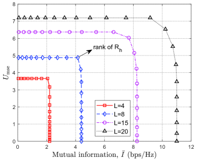
(a) Unlimited power case: $P_{\rm tot}=LP_{\rm ave}$.

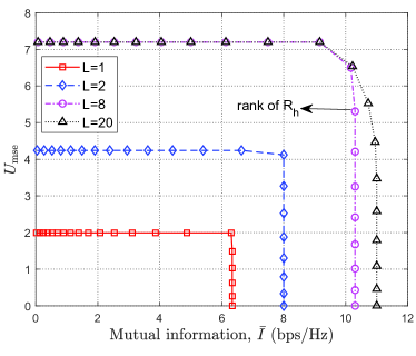
(b) Limited power case: $P_{\rm tot}=T_{c}P_{\rm ave}$.

Figure 3: MSE-MI region for the different length of pilot sequences $L$ under $\delta_{g}^{2}=-90~{}{\rm dBm}$.

IV-A MSE-MI Region of ISAC System

To evaluate the MSE-MI region, we introduce an utility function to describe the normalized MSE of channel $\bf h$ denoted by ${U_{{\rm{mse}}}}=\frac{1}{{{h_{{\rm{NMSE}}}}}}$, where ${{h_{{\rm{NMSE}}}}}$ is given by

$${h_{{\rm{NMSE}}}} =\frac{{{\mathbb{E}}\left\{{{{\left\|{{\bf{h}}-{\bf{\hat{h}}}}\right\|}^{2}}}\right\}}}{{{\mathbb{E}}\left\{{{{\left\|{\bf{h}}\right\|}^{2}}}\right\}}}$$

$$=\frac{{\sigma_{p}^{2}{\rm{tr}}\left({{{\bf{R}}_{\bf{h}}}{{\left({{\bf{X}}_{c}^{H}{{\bf{X}}_{c}}{{\bf{R}}_{\bf{h}}}+\sigma_{p}^{2}{{\bf{I}}_{{N_{t}}}}}\right)}^{-1}}}\right)}}{{{\rm{tr}}\left({{{\bf{R}}_{\bf{h}}}}\right)}}.$$ (108)

It can be seen that a smaller ${{h_{{\rm{NMSE}}}}}$ leads to a larger utility function value ${U_{{\rm{mse}}}}$.

Then, the MSE-MI region is defined as

$${C_{\bar{I}-{{{U}}_{{\rm{mse}}}}}}=\left\{{\left({\bar{I},{{{U}}_{{\rm{mse}}}}}\right):\bar{I}\leq{N_{r}}{{\log}_{2}}\left|{{{\bf{I}}_{L}}{\rm{+}}\frac{{\delta_{g}^{2}}}{{\sigma_{r}^{2}}}{{\bf{X}}_{c}}{\bf{X}}_{c}^{H}}\right|,}\right.$$

$$\!\!\left.{{U_{{\rm{mse}}}}\leq\frac{{{\rm{tr}}\left({{{\bf{R}}_{\bf{h}}}}\right)}}{{\sigma_{p}^{2}{\rm{tr}}\left({{{\bf{R}}_{\bf{h}}}{{\left({{\bf{X}}_{c}^{H}{{\bf{X}}_{c}}{{\bf{R}}_{\bf{h}}}+\sigma_{p}^{2}{{\bf{I}}_{{N_{t}}}}}\right)}^{-1}}}\right)}},\left\|{{{\bf{X}}_{c}}}\right\|_{F}^{2}\leq{P_{{\rm{tot}}}}}\right\},$$ (109)

where ${{P_{{\rm{tot}}}}}$ stands for the power budget. The boundary of ${C_{\bar{I}-{{{U}}_{{\rm{mse}}}}}}$ is called the Pareto boundary, which consists of all the ${\bar{I}}$-${U_{{\rm{mse}}}}$ tuples at which it is impossible to increase ${U_{{\rm{mse}}}}$ without simultaneously decreasing MI, and vice versa [38].

In Fig. 3 (a), we show the MSE-MI region with unlimited power constraint, i.e., ${P_{{\rm{tot}}}}=L{P_{{\rm{ave}}}}$, which indicates that the available power budget is monotonically increasing with $L$. It is observed that the MSE-MI region enlarges as $L$ increases. This is expected since more power can be used for both channel estimation and target detection as $L$ increases. In addition, it is observed that the extreme points on the vertical axis, i.e., the points where the curves intersect the vertical axis, increase with $L$, which is consistent with Remark $1$. Meanwhile, we can see that the extreme points on the horizontal axis also increase with $L$, which is consistent with Remark $2$. Moreover, we can clearly see that there exists a tradeoff between maximizing MI and maximizing ${U_{{\rm{mse}}}}$. Furthermore, we show in Fig. 3 (b) that the MSE-MI region with the limited power constraint, i.e., ${P_{{\rm{tot}}}}=T_{c}{P_{{\rm{ave}}}}$, where ${P_{{\rm{tot}}}}$ is fixed and independent of $L$. It can be observed that the MSE-MI region enlarges when $L\leq{\rm{rank}}\left({{{\bf{R}}_{\bf{h}}}}\right)$, while the ${U_{{\rm{mse}}}}$ will not increase as $L\geq{\rm{rank}}\left({{{\bf{R}}_{\bf{h}}}}\right)$ (see the curves corresponding to $L=8$ and $L=20$). This is because the MSE of the channel will not be further reduced as $L\geq{\rm{rank}}\left({{{\bf{R}}_{\bf{h}}}}\right)$ when the limited power constraint is considered, which is explicitly unveiled in Remark 1.

Figure 4: MSE-MI region comparison for different pilot design approaches under $L=8$ and $\delta_{g}^{2}=-90~{}{\rm dBm}$.

Figure 5: Rate-MI region comparison for different pilot design approaches under $\delta_{g}^{2}=-100~{}{\rm dBm}$ and ${P_{{\rm{ave}}}}=40~{}{\rm dBm}$.

To show the superiority of the proposed pilot structure, we consider the following approaches for comparison.

• Proposed, UPA (unequal power allocation): This is our proposed pilot structure, i.e., ${\bf{X}}_{c}^{H}={{\bf{U}}_{\bf{h}}}\left({1:L}\right){\bf{\Lambda}}$, where ${\bf{\Lambda}}={\rm{diag}}\left({{{\bf{\Lambda}}_{1,1}},\ldots,{{\bf{\Lambda}}_{L,L}}}\right)$ with ${{\bf{\Lambda}}_{i,i}}\geq 0$ needs to be optimized.

• Proposed, EPA (equal power allocation): It is the same as the above scheme except that the power allocation in the main diagonal of ${\bf{\Lambda}}$ is equal, i.e., ${{\bf{\Lambda}}_{1,1}}=\ldots={{\bf{\Lambda}}_{L,L}}$, such that ${{\bf{X}}_{c}}{\bf{X}}_{c}^{H}$ is orthogonal.

• DFT (discrete Fourier transform)-based pilot: The entries in ${{\bf{X}}_{c}}$ are given by ${\left[{{\bf{X}}_{c}}\right]_{i,j}}=\sqrt{P_{\rm DFT}}{e^{-j\frac{{2\pi\left({i-1}\right)\left({j-1}\right)}}{{{N_{t}}}}}},1\leq i\leq L,1\leq j\leq{N_{t}}$, where $P_{\rm DFT}$ represents the allocated power. We have ${{\bf{X}}_{c}}{\bf{X}}_{c}^{H}={P_{{\rm{DFT}}}}{{\bf{I}}_{L}}$, which is orthogonal.

• Gaussian-based pilot: Each entry in ${{\bf{X}}_{c}}$ is independent of each other and follows ${\left[{{\bf{X}}_{c}}\right]_{i,j}}\sim{\cal CN}\left({0,{P_{{\rm{Guassian}}}}}\right),1\leq i\leq L,1\leq j\leq{N_{t}}$, where ${{P_{{\rm{Guassian}}}}}$ represents the power.

• Separate protocol: Stage I is equally divided into two sub-stages. One is for target detection and the other is for channel estimation. The optimal matrices for maximizing the MI and $U_{\rm mse}$ can be directly obtained based on Section III, respectively.

In Fig. 4, we study the MSE-MI tradeoff for different pilot design approaches. It is observed that the MSE-MI region obtained by our proposed pilot structure with UPA is significantly larger than those of the other approaches, which demonstrates the superiority of the proposed pilot design. In addition, we observe that the MSE-MI region obtained by our proposed pilot structure with UPA is larger than that obtained by our proposed pilot structure with EPA since allocating unequal power on pilot sequences can further reduce channel estimation error (equivalently increase ${U_{{\rm{mse}}}}$) shown in (64). Compare the “Proposed, EPA” approach to the DFT-based pilot approach, both pilot structures are orthogonal, whereas the MSE-MI region obtained by the “Proposed, EPA” approach is larger than that obtained by the DFT-based pilot approach. The reason is that the “Proposed, EPA” approach exploits the communication channel information for channel estimation so that the channel estimation error can be further reduced. Furthermore, the Gaussian-based pilot achieves the smallest MSE-MI region since the Gaussian-based pilot is neither orthogonal nor exploiting the communication channel information. It is worth pointing out that all the approaches except the Gaussian-based pilot approach achieves the same maximum MI since the orthogonal pilot matrix is optimal for maximizing the MI. Moreover, compared to “Separate protocol”, we can observe that our proposed scheme significantly outperforms it. This is due to the following two reasons. First, the full time duration can be utilized for the proposed scheme, while only a part of the time duration can be utilized either for target detection or channel estimation. Second, the proposed unified pilot matrix can balance the target detection and channel estimation.

Figure 6: Rate-MI region comparison for the different length of pilot sequences $L$ under $\delta_{g}^{2}=-90~{}{\rm dBm}$.

IV-B Achievable Rate-MI Region of ISAC System

Before proceeding to describe the Rate-MI region, we first define the feasible region of optimization variables $\left\{{{\bf{w}},L,{{\bf{X}}_{c}}}\right\}$ as

$$\!\!\!\Omega=\left\{{\frac{{\left\|{{{\bf{X}}_{c}}}\right\|_{F}^{2}+\left({{T_{c}}-L}\right){{\left\|{\bf{w}}\right\|}^{2}}}}{{{T_{c}}}}\leq{P_{{\rm{ave}}}},0\leq L\leq{T_{c}},L\in{{\mathbb{Z}}^{+}}}\right\}.$$ (110)

As a result, the achievable Rate-MI region is defined as

$$\!\!\!{{\cal C}_{R-\bar{I}}}\overset{\triangle}{=}\left\{{\left({R,\bar{I}}\right):\bar{I}\leq{N_{r}}{{\log}_{2}}\left|{{{\bf{I}}_{L}}{\rm{+}}\frac{{\delta_{g}^{2}}}{{\sigma_{r}^{2}}}{{\bf{X}}_{c}}{\bf{X}}_{c}^{H}}\right|}\right.$$

$$\qquad\qquad\qquad\quad+{N_{r}}\left({{T_{c}}-L}\right){\log_{2}}\left({1+\frac{{\delta_{g}^{2}{{\left\|{\bf{w}}\right\|}^{2}}}}{{\sigma_{r}^{2}}}}\right),$$

$$\!\!\!\!\left.{R\leq\frac{{{T_{c}}-L}}{{{T_{c}}}}{{\log}_{2}}\left({\frac{{{{\bf{w}}^{H}}{{\bf{R}}_{\bf{h}}}{\bf{w}}+\sigma_{t}^{2}}}{{{{\bf{w}}^{H}}{{\bf{R}}_{{{\bf{h}}_{e}}}}{\bf{w}}+\sigma_{t}^{2}}}}\right),{\bf{w}}\in\Omega,L\in\Omega,{{\bf{X}}_{c}}\in\Omega}\right\},$$ (111)

where the $R$-$\bar{I}$ tuples on the Pareto boundary of ${\cal C}_{R-{\bar{I}}}$ can be similarly obtained by Algorithm 1.

In Fig. 5, we compare the Rate-MI tradeoff for different pilot approaches. It is observed that the Rate-MI region obtained by our proposed pilot structure with UPA is larger than the other approaches, which demonstrates the benefit of joint design of the transmit beamformer and pilot sequences. In addition, we observe that the MI is the same for all approaches except the Gaussian-based pilot approach when the required achievable rate is small. This is because as $R$ is small, the minimum rate required by the user can be readily satisfied by just allocating equal power in the pilot training stage and information transmission stage so that the obtained MI $\bar{I}$ is the same. However, for the Gaussian-based pilot approach, since this pilot structure is not orthogonal, the performance of MI will be impaired and thus, a performance degradation is incurred.

Figure 7: $\bar{I}$ versus $P_{\rm ave}$ under $R_{\rm th}=2~{}{\rm bps/Hz}$, $\beta_{\rm rician}=-\infty$ (in dB), $d=100~{}{\rm m}$, $r=0.8$, and $\alpha=2.6$.

In Fig. 6, we compare the Rate-MI tradeoff for different $L$. It is observed that the Rate-MI region firstly enlarges as $L$ increases (see curves from $L=2$ to $L=4$), and then shrinks when $L$ becomes large (see curves from $L=8$ to $L=12$). This is because the effective spectral efficiency of the user is affected by two factors: 1) the duration time $L$ for channel estimation and 2) the duration time $T_{c}-L$ for information transmission. As $L$ is small, the channel estimation error is large, and the achievable rate is small even if the remaining duration time, i.e., $T_{c}-L$, for information transmission is large. In contrast, as $L$ becomes large, the channel estimation error is significantly reduced, whereas the achievable rate is still small since the remaining time for information transmission is small. Interestingly, we can see that $L{\rm{=rank}}\left({{{\bf{R}}_{\bf{h}}}}\right)$ is not the optimal pilot sequence length to maximize the Rate-MI region. Therefore, there exists a tradeoff between minimizing the channel estimation error and maximizing the user’s effective throughput.

In Fig. 7, we compare the MI obtained by different approaches versus $P_{\rm ave}$. The following benchmark approaches are compared: 1) Fixed power allocation: Similar to the proposed approach except that the power allocated to two stages, i.e., the channel estimation stage and the information transmission stage, is the same; 2) $L{\rm{=rank}}\left({{{\bf{R}}_{\bf{h}}}}\right)$: Similar to the proposed approach except that the pilot length is fixed with $L{\rm{=rank}}\left({{{\bf{R}}_{\bf{h}}}}\right)$; 3) Gaussian-based pilot: Similar to the proposed approach except that each entry in ${\bf{X}}_{c}^{H}$ is CSCG distributed. 4) Separate S&C: The coherence time is divided into three stages, namely target detection, channel estimation, and information transmission. The optimal sensing matrix for target detection and the optimal pilot matrix for channel estimation can be easily derived in closed-form expressions, while the beamformer can be similarly solved by the proposed Algorithm 1. It is observed that the MI for all approaches increases monotonically with $P_{\rm ave}$ as expected. In addition, we observe that the proposed approach outperforms the other benchmark approaches, which indicates the benefits of joint design of pilot design and transmit beamformer. To show the impact of MI on the target detection performance, the corresponding $P_{d}$ versus $P_{\rm ave}$ is studied in Fig. 8. We first obtain the solution based on the MI maximization optimization problem, and then substitute the obtained pilot matrix, transmit beamformer, and training duration into (33a) to obtain the corresponding target detection probability. Compared to Fig. 7, we observe that a higher MI corresponds to a higher target detection probability, which demonstrates that maximizing the MI potentially increases the detection probability. Moreover, we can observe that the “Separate S&C” scheme achieves very low detection probability even as power budget is large. This is because only a part of the time is utilized for target detection. In contrast, our proposed scheme achieves much higher detection probability than the “Separate S&C” scheme, which implies that the proposed protocol outperforms the separate protocol. The reason is that full-time duration and a well-customized pilot matrix are leveraged in our proposed scheme.

Figure 8: $P_{d}$ versus $P_{\rm ave}$ under $R_{\rm th}=2~{}{\rm bps/Hz}$, $\beta_{\rm rician}=-\infty$ (in dB), $d=100~{}{\rm m}$, $r=0.8$, and $\alpha=2.6$.

Figure 9: Rate-MI region for different correlation coefficients $\left\{{r=0.3,r=0.5,r=0.9}\right\}$ under ${P_{{\rm{ave}}}}=40~{}{\rm dBm}$, $\sigma^{2}=-90~{}{\rm dBm}$, $d=100~{}{\rm m}$, and a path loss exponent of $2.6$.

In Fig. 9, we study the Rate-MI tradeoff for different correlation coefficients $r$ under $\beta_{\rm rician}=-\infty$ (in dB) and $\beta_{\rm rician}=3~{}{\rm dB}$. It is observed that the Rate-MI region enlarges as $r$ increases. This is because as $r$ increases, the communication channel becomes more spatially correlated and the rank of its covariance matrix, i.e., ${\rm{rank}}\left({{{\bf{R}}_{\bf{h}}}}\right)$, becomes smaller. Therefore, the need of the length of pilot sequences for channel estimation is reduced and the remaining duration for information transmission increases, and the effective spectral efficiency of user is thus increased. In addition, with the same correlation coefficient, i.e., $r=0.9$, a larger ${{\beta_{{\rm{rician}}}}}$ leads to a larger Rate-MI region. This is because as ${{\beta_{{\rm{rician}}}}}$ increases, the communication channel becomes more spatially correlated and the rank of ${\rm{rank}}\left({{{\bf{R}}_{\bf{h}}}}\right)$ is also reduced so that the effective spectral efficiency of user improves.

V Conclusion

In this paper, we investigated the performance limit of ISAC by studying the MSE-MI and Rate-MI regions. We proposed a novel target detection and information transmission protocol where both channel estimation and information transmission stages are leveraged for target detection. The corresponding target detection probability was derived by applying the GLRT-based detector. By respectively designing the optimal pilot matrix for the channel estimation and target detection, the fundamental tradeoff between minimizing the channel estimation error and maximizing MI was unveiled and a novel pilot structure was then proposed to balance the above two functionalities. In addition, the impact of training duration on channel estimation and target detection was characterized. Finally, we proposed an efficient iterative algorithm to maximize MI by jointly optimizing the pilot matrix, the training duration, and the transmit beamformer. Extensive simulation results under various practical setups demonstrated that our proposed pilot structure can well balance the system performance between the communication transmission and the target detection, and by jointly optimizing the pilot matrix and transmit beamformer, the Rate-MI region can be significantly enlarged. Furthermore, it was also unveiled that as the communication channel is more spatially correlated, the Rate-MI region can be further enlarged.

Appendix A Proof of Lemma 2

Let ${\bf{X}}={{\bf{U}}_{\bf{x}}}{{\bf{\Sigma}}_{\bf{x}}}{\bf{V}}_{\bf{x}}^{H}$ by performing (reduced) singular value decomposition on ${\bf{X}}$, where ${{\bf{U}}_{\bf{x}}}\in{{\mathbb{C}}^{{T_{c}}\times\upsilon}},{{\bf{\Sigma}}_{\bf{x}}}\in{\mathbb{C}^{\upsilon\times\upsilon}},{\bf{V}}_{\bf{x}}^{H}\in{\mathbb{C}^{\upsilon\times{N_{t}}}}$, and $\upsilon=\min\left({L+1,{N_{t}}}\right)$, with ${\bf{U}}_{\bf{x}}^{H}{{\bf{U}}_{\bf{x}}}={{\bf{I}}_{{T_{c}}}}$, ${\bf{V}}_{\bf{x}}^{H}{{\bf{V}}_{\bf{x}}}={{\bf{I}}_{{N_{t}}}}$, ${{\bf{\Sigma}}_{\bf{x}}}={\rm{diag}}\left({{{\bf{\Sigma}}_{1,1}},\ldots,{{\bf{\Sigma}}_{\upsilon}}}\right)$, and ${{\bf{\Sigma}}_{1,1}}\geq\ldots{{\bf{\Sigma}}_{\upsilon,\upsilon}}>0$. Thus, we have ${\left({{{\bf{X}}^{H}}{\bf{X}}}\right)^{\dagger}}={{\bf{V}}_{\bf{x}}}{\bf{\Sigma}}_{\bf{x}}^{-2}{\bf{V}}_{\bf{x}}^{H}$. Then, substituting it into ${\rm{rank}}\left({{\bf{X}}{{\left({{{\bf{X}}^{H}}{\bf{X}}}\right)}^{\dagger}}{{\bf{X}}^{H}}}\right)$ yields

$${\rm{rank}}\left({{\bf{X}}{{\left({{{\bf{X}}^{H}}{\bf{X}}}\right)}^{\dagger}}{{\bf{X}}^{H}}}\right)$$

$$={\rm{rank}}\left({{{\bf{U}}_{\bf{x}}}{{\bf{\Sigma}}_{\bf{x}}}{\bf{V}}_{\bf{x}}^{H}{{\bf{V}}_{\bf{x}}}{\bf{\Sigma}}_{\bf{x}}^{-2}{\bf{V}}_{\bf{x}}^{H}{{\bf{V}}_{\bf{x}}}{{\bf{\Sigma}}_{\bf{x}}}{\bf{U}}_{\bf{x}}^{H}}\right)$$

$$={\rm{rank}}\left({{{\bf{U}}_{\bf{x}}}{\bf{U}}_{\bf{x}}^{H}}\right)={\rm{rank}}\left({{{\bf{U}}_{\bf{x}}}}\right)=\min\left({L+1,{N_{t}}}\right)$$

$$\overset{\triangle}{=}{\rm{rank}}\left({\bf{X}}\right).$$ (112)

This thus completes the proof of Lemma $2$.

Appendix B Proof of Lemma 3

We first check ${\bf{X}}{\left({{{\bf{X}}^{H}}{\bf{X}}}\right)^{\dagger}}{{\bf{X}}^{H}}$ is idempotent, i.e., ${\left({{\bf{X}}{{\left({{{\bf{X}}^{H}}{\bf{X}}}\right)}^{\dagger}}{{\bf{X}}^{H}}}\right)^{2}}={\bf{X}}{\left({{{\bf{X}}^{H}}{\bf{X}}}\right)^{\dagger}}{{\bf{X}}^{H}}$. Recall that ${\left({{{\bf{X}}^{H}}{\bf{X}}}\right)^{\dagger}}={{\bf{V}}_{\bf{x}}}{\bf{\Sigma}}_{\bf{x}}^{-2}{\bf{V}}_{\bf{x}}^{H}$ (see it in Appendix A), we can obtain ${\bf{X}}{\left({{{\bf{X}}^{H}}{\bf{X}}}\right)^{\dagger}}{{\bf{X}}^{H}}={{\bf{U}}_{\bf{x}}}{\bf{U}}_{\bf{x}}^{H}$. Then, we can express ${\left({{\bf{X}}{{\left({{{\bf{X}}^{H}}{\bf{X}}}\right)}^{\dagger}}{{\bf{X}}^{H}}}\right)^{2}}$ as

$${\left({{\bf{X}}{{\left({{{\bf{X}}^{H}}{\bf{X}}}\right)}^{\dagger}}{{\bf{X}}^{H}}}\right)^{2}} ={{\bf{U}}_{\bf{x}}}{{\bf{\Sigma}}_{\bf{x}}}{\bf{V}}_{\bf{x}}^{H}{{\bf{V}}_{\bf{x}}}{\bf{\Sigma}}_{\bf{x}}^{-2}{\bf{V}}_{\bf{x}}^{H}{{\bf{V}}_{\bf{x}}}{{\bf{\Sigma}}_{\bf{x}}}{\bf{U}}_{\bf{x}}^{H}$$

$$\times{{\bf{U}}_{\bf{x}}}{{\bf{\Sigma}}_{\bf{x}}}{\bf{V}}_{\bf{x}}^{H}{{\bf{V}}_{\bf{x}}}{\bf{\Sigma}}_{\bf{x}}^{-2}{\bf{V}}_{\bf{x}}^{H}{{\bf{V}}_{\bf{x}}}{{\bf{\Sigma}}_{\bf{x}}}{\bf{U}}_{\bf{x}}^{H}$$

$$={{\bf{U}}_{\bf{x}}}{\bf{U}}_{\bf{x}}^{H},$$ (113)

which indicates that ${\left({{\bf{X}}{{\left({{{\bf{X}}^{H}}{\bf{X}}}\right)}^{\dagger}}{{\bf{X}}^{H}}}\right)^{2}}={\bf{X}}{\left({{{\bf{X}}^{H}}{\bf{X}}}\right)^{\dagger}}{{\bf{X}}^{H}}$ and is thus idempotent.

Next, we prove that the eigenvalue of ${\bf{X}}{\left({{{\bf{X}}^{H}}{\bf{X}}}\right)^{\dagger}}{{\bf{X}}^{H}}$ is either $0$ or $1$. Let ${\bf{M}}={\bf{X}}{\left({{{\bf{X}}^{H}}{\bf{X}}}\right)^{\dagger}}{{\bf{X}}^{H}}$ and $\lambda$ and $\bf a$ (${\bf{a}}\neq{\bf{0}}$) be its eigenvalue and eigenvector, respectively. As such, we have

$${\bf{Ma}}=\lambda{\bf{a}}\Rightarrow{{\bf{M}}^{2}}{\bf{a}}=\lambda{\bf{Ma}}\Rightarrow\lambda\left({1-\lambda}\right){\bf{a}}={\bf{0}}.$$ (114)

Thus, $\lambda$ is equal to either $0$ or $1$. In addition, since ${\rm{rank}}\left({{\bf{X}}{{\left({{{\bf{X}}^{H}}{\bf{X}}}\right)}^{\dagger}}{{\bf{X}}^{H}}}\right)={\rm{rank}}\left({\bf{X}}\right)=\min\left({L+1,{N_{t}}}\right)$, the number of non-zeros is $\min\left({L+1,{N_{t}}}\right)$. Based on these, we complete the proof of Lemma $3$.

References

• [1] J. A. Zhang, M. L. Rahman, K. Wu, X. Huang, Y. J. Guo, S. Chen, and J. Yuan, “Enabling joint communication and radar sensing in mobile networks-A survey,” IEEE Commun. Surveys Tuts., vol. 24, no. 1, pp. 306–345, 1st Quat. 2022.
• [2] S. Aheleroff, X. Xu, Y. Lu, M. Aristizabal, J. Pablo Velásquez, B. Joa, and Y. Valencia, “IoT-enabled smart appliances under industry 4.0: A case study,” Adv. Eng. Inform., vol. 43, p. 101043, Jan. 2020.
• [3] G. Chen, Q. Wu, W. Chen, D. W. K. Ng, and L. Hanzo, “IRS-aided wireless powered MEC systems: TDMA or NOMA for computation offloading?” IEEE Trans. Wireless Commun., vol. 22, no. 2, pp. 1201–1218, Feb. 2023.
• [4] Statista, Accessed on Sept., 26, 2022. [Online]. Available: https://www.statista.com/statistics/1183457/iot-connected-devices-worldwide/.
• [5] A. Liu, Z. Huang, M. Li, Y. Wan, W. Li, T. X. Han, C. Liu, R. Du, D. K. P. Tan, J. Lu, Y. Shen, F. Colone, and K. Chetty, “A survey on fundamental limits of integrated sensing and communication,” IEEE Commun. Surveys Tuts., vol. 24, no. 2, pp. 994–1034, 2nd Quat. 2022.
• [6] D. Ma, N. Shlezinger, T. Huang, Y. Liu, and Y. C. Eldar, “Joint radar-communication strategies for autonomous vehicles: Combining two key automotive technologies,” IEEE Signal Process. Mag., vol. 37, no. 4, pp. 85–97, Jul. 2020.
• [7] N. C. Luong, X. Lu, D. T. Hoang, D. Niyato, and D. I. Kim, “Radio resource management in joint radar and communication: A comprehensive survey,” IEEE Commun. Surveys Tuts., vol. 23, no. 2, pp. 780–814, 2nd Quart. 2021.
• [8] F. Liu, C. Masouros, A. P. Petropulu, H. Griffiths, and L. Hanzo, “Joint radar and communication design: Applications, state-of-the-art, and the road ahead,” IEEE Trans. Commun., vol. 68, no. 6, pp. 3834–3862, Jun. 2020.
• [9] Y. Chen, H. Hua, and J. Xu, “ISAC meets SWIPT: Multi-functional wireless systems integrating sensing, communication, and powering,” 2022. [Online]. Available: https://arxiv.org/abs/2211.10605.
• [10] Y. Liu, I. Al-Nahhal, O. A. Dobre, and F. Wang, “Deep-learning channel estimation for IRS-assisted integrated sensing and communication system,” IEEE Trans. Veh. Technol., vol. 72, no. 5, pp. 6181–6193, May 2023.
• [11] Y. Cui, F. Liu, X. Jing, and J. Mu, “Integrating sensing and communications for ubiquitous IoT: Applications, trends, and challenges,” IEEE Network, vol. 35, no. 5, pp. 158–167, Sept. 2021.
• [12] A. Hassanien, M. G. Amin, Y. D. Zhang, and F. Ahmad, “Dual-function radar-communications: Information embedding using sidelobe control and waveform diversity,” IEEE Tran. Signal Process., vol. 64, no. 8, pp. 2168–2181, Apr. 2016.
• [13] ——, “Phase-modulation based dual-function radar-communications,” IET Radar, Sonar Navigation, vol. 10, no. 8, pp. 1411–1421, Oct. 2016.
• [14] X. Wang, A. Hassanien, and M. G. Amin, “Sparse transmit array design for dual-function radar communications by antenna selection,” Digit. Signal Process., vol. 83, pp. 223–234, Dec. 2018.
• [15] C. Sturm and W. Wiesbeck, “Waveform design and signal processing aspects for fusion of wireless communications and radar sensing,” Proc. IEEE, vol. 99, no. 7, pp. 1236–1259, Jul. 2011.
• [16] Y. L. Sit, C. Sturm, and T. Zwick, “Doppler estimation in an OFDM joint radar and communication system,” in Proc. German Microw.Conf., Ilmenau, Germany, 2011, pp. 1–4.
• [17] K. M. Braun, “OFDM radar algorithms in mobile communication networks,” Ph.D. dissertation, Karlsruhe, Karlsruher Institut für Technologie (KIT), Diss., 2014.
• [18] M. Hua, Q. Wu, C. He, S. Ma, and W. Chen, “Joint active and passive beamforming design for IRS-aided radar-communication,” IEEE Trans. Wireless Commun., vol. 22, no. 4, pp. 2278–2294, Apr. 2023.
• [19] X. Liu, T. Huang, N. Shlezinger, Y. Liu, J. Zhou, and Y. C. Eldar, “Joint transmit beamforming for multiuser MIMO communications and MIMO radar,” IEEE Trans. Signal Process., vol. 68, pp. 3929–3944, Jun. 2020.
• [20] F. Liu, L. Zhou, C. Masouros, A. Li, W. Luo, and A. Petropulu, “Toward dual-functional radar-communication systems: Optimal waveform design,” IEEE Trans. Signal Process., vol. 66, no. 16, pp. 4264–4279, Aug. 2018.
• [21] H. Hua, J. Xu, and T. X. Han, “Optimal transmit beamforming for integrated sensing and communication,” IEEE Trans. Veh. Technol., vol. 72, no. 8, pp. 10 588–10 603, Aug. 2023.
• [22] H. Luo, R. Liu, M. Li, Y. Liu, and Q. Liu, “Joint beamforming design for RIS-assisted integrated sensing and communication systems,” IEEE Trans. Veh. Technol., vol. 71, no. 12, pp. 13 393–13 397, Dec. 2022.
• [23] A. De Maio and M. Lops, “Design principles of MIMO radar detectors,” IEEE Trans. Aerosp Electron Syst., vol. 43, no. 3, pp. 886–898, Jul. 2007.
• [24] Y. Gu and Y. D. Zhang, “Information-theoretic pilot design for downlink channel estimation in FDD massive MIMO systems,” EEE Trans. Signal Process., vol. 67, no. 9, pp. 2334–2346, May 2019.
• [25] Z. Huang, K. Wang, A. Liu, Y. Cai, R. Du, and T. X. Han, “Joint pilot optimization, target detection and channel estimation for integrated sensing and communication systems,” IEEE Trans. Wireless Commun., vol. 21, no. 12, pp. 10 351–10 365, Dec. 2022.
• [26] L. Xu, J. Li, and P. Stoica, “Target detection and parameter estimation for MIMO radar systems,” IEEE Trans. Aerosp. Electron. Syst., vol. 44, no. 3, pp. 927–939, Jul. 2008.
• [27] E. Fishler, A. Haimovich, R. Blum, L. Cimini, D. Chizhik, and R. Valenzuela, “Spatial diversity in radars—models and detection performance,” IEEE Trans. Signal Process., vol. 54, no. 3, pp. 823–838, Mar. 2006.
• [28] J. G. Proakis, “Digital communications fourth edition,” McGraw-Hill Companies, Inc., New York, NY, 2001.
• [29] D. Samardzija and N. Mandayam, “Pilot-assisted estimation of MIMO fading channel response and achievable data rates,” IEEE Tran. Signal Process., vol. 51, no. 11, pp. 2882–2890, Nov. 2003.
• [30] V. Havary-Nassab, S. Shahbazpanahi, A. Grami, and Z.-Q. Luo, “Distributed beamforming for relay networks based on second-order statistics of the channel state information,” EEE Tran. Signal Process., vol. 56, no. 9, pp. 4306–4316, Sept. 2008.
• [31] Y. Cao and C. Tellambura, “Joint distributed beamforming and power allocation in underlay cognitive two-way relay links using second-order channel statistics,” IEEE Trans. Signal Process., vol. 62, no. 22, pp. 5950–5961, Nov. 2014.
• [32] D. Ponukumati, F. Gao, and M. Bode, “Robust multicell downlink beamforming based on second-order statistics of channel state information,” in Proc. IEEE Glob. Telecommun (GLOBECOM),Houston, Texas, USA,, Dec. 2012, pp. 1–5.
• [33] D. Palomar, J. Cioffi, and M. Lagunas, “Joint Tx-Rx beamforming design for multicarrier MIMO channels: A unified framework for convex optimization,” IEEE Tran. Signal Process., vol. 51, no. 9, pp. 2381–2401, Sept. 2003.
• [34] S. Boyd and L. Vandenberghe, Convex Optimization.   Cambridge University Press, 2004.
• [35] J. Gondzio and T. Terlaky, “A computational view of interior point methods,” Advances in Linear and Integer Programming. Oxford Lecture Series in Mathematics and its Applications, vol. 4, pp. 103–144, 1996.
• [36] M.-M. Zhao, Q. Wu, M.-J. Zhao, and R. Zhang, “Intelligent reflecting surface enhanced wireless networks: Two-timescale beamforming optimization,” IEEE Trans. Wireless Commun., vol. 20, no. 1, pp. 2–17, Jan. 2021.
• [37] S. Loyka, “Channel capacity of MIMO architecture using the exponential correlation matrix,” IEEE Commun. Lett., vol. 5, no. 9, pp. 369–371, Sept. 2001.
• [38] E. A. Jorswieck, E. G. Larsson, and D. Danev, “Complete characterization of the pareto boundary for the MISO interference channel,” IEEE Tran. Signal Process., vol. 56, no. 10, pp. 5292–5296, Oct. 2008.