The fractional Landau-Lifshitz-Gilbert equation

Abstract

The dynamics of a magnetic moment or spin are of high interest to applications in technology. Dissipation in these systems is therefore of importance for improvement of efficiency of devices, such as the ones proposed in spintronics. A large spin in a magnetic field is widely assumed to be described by the Landau-Lifshitz-Gilbert (LLG) equation, which includes a phenomenological Gilbert damping. Here, we couple a large spin to a bath and derive a generic (non-)Ohmic damping term for the low-frequency range using a Caldeira-Leggett model. This leads to a fractional LLG equation, where the first-order derivative Gilbert damping is replaced by a fractional derivative of order $s\geq 0$. We show that the parameter $s$ can be determined from a ferromagnetic resonance experiment, where the resonance frequency and linewidth no longer scale linearly with the effective field strength.

Introduction.— The magnetization dynamics of materials has attracted much interest because of its technological applications in spintronics, such as data storage or signal transfer [1, 2, 3]. The right-hand rule of magnetic forces implies that the basic motion of a magnetic moment or macrospin $\bm{S}$ in a magnetic field $\bm{B}$ is periodic precession. However, coupling to its surrounding (e.g., electrons, phonons, magnons, and impurities) will lead to dissipation, which will align $\bm{S}$ with $\bm{B}$.

Spintronics-based devices use spin waves to carry signals between components [4]. Contrary to electronics, which use the flow of electrons, the electrons (or holes) in spintronics remain stationary and their spin degrees of freedom are used for transport. This provides a significant advantage in efficiency, since the resistance of moving particles is potentially much larger than the dissipation of energy through spins. The spin waves consist of spins precessing around a magnetic field and they are commonly described by the Landau-Lifshitz-Gilbert (LLG) equation [5]. This phenomenological description also includes Gilbert damping, which is a term that slowly realigns the spins with the magnetic field. Much effort is being done to improve the control of spins for practical applications [6]. Since efficiency is one of the main motivations to research spintronics, it is important to understand exactly what is the dissipation mechanism of these spins.

Although the LLG equation was first introduced phenomenologically, since then it has also been derived from microscopic quantum models [7, 8]. Quantum dissipation is a topic of long debate, since normal Hamiltonians will always have conservation of energy. It can be described, for instance, with a Caldeira-Leggett type model [9, 10, 11, 12, 13], where the Hamiltonian of the system is coupled to a bath of harmonic oscillators. These describe not only bosons, but any degree of freedom of an environment in equilibrium. These oscillators can be integrated out, leading to an effective action of the system that is non-local and accounts for dissipation. The statistics of the bath is captured by the spectral function $J(\omega)$, which determines the type of dissipation. For a linear spectral function (Ohmic bath), the first-order derivative Gilbert damping is retrieved.

The spectral function is usually very difficult to calculate or measure, so it is often assumed for simplicity that the bath is Ohmic. However, $J(\omega)$ can have any continuous shape. Hence, a high frequency cutoff is commonly put in place, which sometimes justifies a linear expansion. However, a general expansion is that of an $s$ order power-law, where $s$ could be any positive real number. A spectral function with such a power-law is called non-Ohmic, and we refer to $s$ as the “Ohmicness” of the bath. It is known that non-Ohmic baths exist [14, 15, 16, 17, 18, 19, 20, 21, 22, 23] and that they can lead to equations of motion that include fractional derivatives [24, 25, 26, 27, 28]. Because fractional derivatives are non-local, these systems show non-Markovian dynamics which can be useful to various applications [29, 30, 31].

Here, we show that a macroscopic spin in contact with a non-Ohmic environment leads to a fractional LLG equation, where the first derivative Gilbert damping gets replaced by a fractional Liouville derivative. Then, we explain how experiments can use ferromagnetic resonance (FMR) to determine the Ohmicness of their environment from resonance frequency and/or linewidth. This will allow experiments to stop using the Ohmic assumption, and use equations based on measured quantities instead. The same FMR measurements can also be done with anisotropic systems. Aligning anisotropy with the magnetic field may even aid the realization of measurements, as this can help reach the required effective field strengths. In practice, the determination of the type of environment is challenging, since one needs to measure the coupling strength with everything around the spins. However, with the experiment proposed here, one can essentially measure the environment through the spin itself. Therefore, the tools that measure spins can now also be used to determine the environment. This information about the dissipation may lead to improved efficiency, stability, and control of applications in technology.

Derivation of a generalized LLG equation.— We consider a small ferromagnet that is exposed to an external magnetic field. Our goal is to derive an effective equation of motion for the magnetization. For simplicity, we model the magnetization as one large spin (macrospin) $\hat{\bm{S}}$. Its Hamiltonian (note that we set $\hbar$ and $k_{B}$ to one) reads $\hat{H}_{s}=\bm{B}\cdot\hat{\bm{S}}-K\hat{S}_{z}^{2}$, where the first term (Zeeman) describes the coupling to the external magnetic field $\bm{B}$, and the second term accounts for (axial) anisotropy of the magnet. However, since a magnet consists of more than just a magnetization, the macrospin will be in contact with some environment. Following the idea of the Caldeira-Leggett approach [9, 10, 11, 12, 32, 13], we model the environment as a bath of harmonic oscillators, $\hat{H}_{b}=\sum_{\alpha}\hat{\bm{p}}_{\alpha}^{2}/2m_{\alpha}+m_{\alpha}\omega_{\alpha}^{2}\hat{\bm{x}}_{\alpha}^{2}/2$, where $\hat{\bm{x}}_{\alpha}$ and $\hat{\bm{p}}_{\alpha}$ are position and momentum operators of the $\alpha$-th bath oscillator with mass $m_{\alpha}$ and eigenfrequency $\omega_{\alpha}>0$. Furthermore, we assume the coupling between the macrospin and the bath modes to be linear, $\hat{H}_{c}=\sum_{\alpha}\gamma_{\alpha}\,\hat{\bm{S}}\cdot\hat{\bm{x}}_{\alpha}$, where $\gamma_{\alpha}$ is the coupling strength between macrospin and the $\alpha$-th oscillator. Thus, the full Hamiltonian of macrospin and environment is given by $\hat{H}=\hat{H}_{s}+\hat{H}_{c}+\hat{H}_{b}$.

Next, we use the Keldysh formalism in its path-integral version [33, 34], which allows us to derive an effective action and, by variation, an effective quasi-classical equation of motion for the macrospin. For the path-integral representation of the macrospin, we use spin coherent states [34] $\lvert g\rangle=\exp(-i\phi\hat{S}_{z})\exp(-i\theta\hat{S}_{y})\exp(-i\psi\hat{S}_{z})\,\lvert\uparrow\rangle$, where $\phi$, $\theta$, and $\psi$ are Euler angles and $\lvert\uparrow\rangle$ is the eigenstate of $\hat{S}_{z}$ with the maximal eigenvalue $S$. Spin coherent states provide an intuitive way to think about the macrospin as a simple vector $\bm{S}=\langle g\rvert\hat{\bm{S}}\lvert g\rangle=S\,(\sin\theta\cos\phi,\sin\theta\sin\phi,\cos\theta)$ with constant length $S$ and the usual angles for spherical coordinates $\theta$ and $\phi$. For spins, the third Euler angle $\psi$ presents a gauge freedom, which we fix as in Ref. [35] for the same reasons explained there.

After integrating out the bath degrees of freedom, see Sup. Mat. [36] for details, we obtain the Keldysh partition function $\mathcal{Z}=\int Dg\,\exp[i\mathcal{S}]$, with the Keldysh action

$$\mathcal{S}= \oint\!dt\,\big{[}S\,\dot{\phi}\,(1-\cos\theta)-\bm{B}_{\mathrm{eff}}(S_{z})\cdot\bm{S}\big{]}$$

$$-\oint\!dt\oint\!dt^{\prime}\ \bm{S}(t)\,\alpha(t-t^{\prime})\,\bm{S}(t^{\prime})\ .$$ (1)

The first term, called Berry connection, takes the role of a kinetic energy for the macrospin; it arises from the time derivative acting on the spin coherent states $(-i\partial_{t}\langle g\rvert)\lvert g\rangle=S\,\dot{\phi}\,(1-\cos\theta)$. The second term is the potential energy of the macrospin, where we introduced an effective magnetic field, $\bm{B}_{\mathrm{eff}}(S_{z})=\bm{B}-KS_{z}\,\bm{e}_{z}$, given by the external magnetic field and the anisotropy. The third term arises from integrating out the bath and accounts for the effect of the environment onto the macrospin; that is, the kernel function $\alpha(t-t^{\prime})$ contains information about dissipation and fluctuations. Dissipation is described by the retarded and advanced components $\alpha^{R/A}(\omega)=\sum_{\alpha}(\gamma_{\alpha}^{2}/2m_{\alpha}\omega_{\alpha}^{2})\,\omega^{2}/[(\omega\pm i0)^{2}-\omega_{\alpha}^{2}]$, whereas the effect of fluctuations is included in the Keldysh component, $\alpha^{K}(\omega)=\coth(\omega/2T)\,[\alpha^{R}(\omega)-\alpha^{A}(\omega)]$. This is determined by the fluctuation-dissipation theorem, as we assume the bath to be in a high-temperature equilibrium state [37, 33, 34].

From the Keldysh action, Eq. (1), we can now derive an equation of motion for the macrospin by taking a variation. More precisely, we can derive quasi-classical equations of motion for the classical components of the angles $\theta$ and $\phi$ by taking the variation with respect to their quantum components [38]. The resulting equations of motion can be recast into a vector form and lead to a generalized LLG equation

$$\dot{\bm{S}}(t)=\bm{S}(t)\times\left[-\bm{B}_{\mathrm{eff}}[S_{z}(t)]+\int_{-\infty}^{t}\!\!\!\!dt^{\prime}\,\alpha(t-t^{\prime})\,\bm{S}(t^{\prime})+\bm{\xi}(t)\right],$$ (2)

with the dissipation kernel [39] given by

$$\alpha(\omega)=\int_{-\infty}^{\infty}\frac{d\varepsilon}{\pi}\frac{\varepsilon J(\varepsilon)}{(\omega+i0)^{2}-\varepsilon^{2}}\ ,$$ (3)

where we introduced the bath spectral density $J(\omega)=\sum_{\alpha}(\pi\gamma_{\alpha}^{2}/2m_{\alpha}\omega_{\alpha})\,\delta(\omega-\omega_{\alpha})$ [33, 36]. The last term in Eq. (2) contains a stochastic field $\bm{\xi}(t)$, which describes fluctuations (noise) caused by the coupling to the bath; the noise correlator for the components of $\bm{\xi}(t)$ is given by $\langle\xi_{m}(t)\xi_{n}(t^{\prime})\rangle=-2i\,\delta_{mn}\,\alpha^{K}(t-t^{\prime})$. Next, to get a better understanding of the generalized LLG equation, we consider some examples of bath spectral densities.

Fractional Landau-Lifshitz-Gilbert equation.— For the generalized LLG equation (2), it is natural to ask: In which case do we recover the standard LLG equation? We can recover it for a specific choice of the bath spectral density $J(\omega)$, which we introduced in Eq. (3). Roughly speaking, $J(\omega)$ describes two things: first, in the delta function $\delta(\omega-\omega_{\alpha})$, it describes at which energies $\omega_{\alpha}$ the macrospin can interact with the bath; second, in the prefactor $\pi\gamma_{\alpha}^{2}/2m_{\alpha}\omega_{\alpha}$, it describes how strongly the macrospin can exchange energy with the bath at the frequency $\omega_{\alpha}$. In our simple model, the bath spectral density is a sum over $\delta$-peaks because we assumed excitations of the bath oscillators to have an infinite life time. However, also the bath oscillators will have some dissipation of their own, such that the $\delta$-peaks will be broadened. If, furthermore, the positions of the bath-oscillator frequencies $\omega_{\alpha}$ is dense on the scale of their peak broadening, the bath spectral density becomes a continuous function instead of a collection of $\delta$-peaks. In the following, we focus on cases where the bath spectral density is continuous.

Since the bath only has positive frequencies, we have $J(\omega\leq 0)=0$. Even though $J(\omega)$ can have any positive continuous shape, one might assume that it is an approximately linear function at low frequencies; that is,

$$J(\omega)=\alpha_{1}\,\omega\,\Theta(\omega)\Theta(\Omega_{c}-\omega),$$ (4)

where $\Theta(\omega)=1$ for $\omega>0$ and $\Theta(\omega)=0$ for $\omega<0$ and $\Omega_{c}$ is some large cutoff frequency of the bath such that we have $\omega_{\text{system}}\ll T\ll\Omega_{c}$. Reservoirs with such a linear spectral density are also known as Ohmic baths. Inserting the Ohmic bath spectral density back into Eq. (3), while sending $\Omega_{c}\to\infty$, we recover the standard LLG equation,

$$\dot{\bm{S}}(t)=\bm{S}(t)\times\left[-\bm{B}_{\mathrm{eff}}[S_{z}(t)]+\alpha_{1}\dot{\bm{S}}(t)+\bm{\xi}(t)\right],$$ (5)

where the first term describes the macrospin’s precession around the effective magnetic field, the second term—known as Gilbert damping—describes the dissipation of the macrospin’s energy and angular momentum into the environment, and the third term describes the fluctuations with $\langle\xi_{m}(t)\xi_{n}(t^{\prime})\rangle=4\alpha_{1}T\,\delta_{mn}\,\delta(t-t^{\prime})$, which are related to the Gilbert damping by the fluctuation-dissipation theorem. Note that the same results can be obtained without a cutoff frequency by introducing a counter term, which effectively only changes the zero-energy level of the bath, see Sup. Mat. [36] for details.

The assumption of an Ohmic bath can sometimes be justified, but is often chosen out of convenience, as it is usually the simplest bath type to consider. To our knowledge, there has been little to no experimental verification whether the typical baths of magnetizations in ferromagnets are Ohmic or not. To distinguish between Ohmic and non-Ohmic baths, we need to know how the magnetization dynamics depends on that difference. Hence, instead of the previous assumption of a linear bath spectral density (Ohmic bath), we now assume that the bath spectral density has a power-law behavior at low frequencies,

$$J(\omega)=\tilde{\alpha}_{s}\omega^{s}\,\Theta(\omega)\Theta(\Omega_{c}-\omega)\ ,$$ (6)

where we refer to $s$ as Ohmicness parameter [40]. It is convenient to define $\alpha_{s}=\tilde{\alpha}_{s}/\sin(\pi s/2)$ and we should note that the dimension of $\alpha_{s}$ depends on $s$. For $s=1$ we recover the Ohmic bath. Correspondingly, baths with $s<1$ are called sub-Ohmic and baths with $s>1$ are called super-Ohmic. For $0<s<2$ and $\Omega_{c}\to\infty$, we find the fractional LLG equation

$$\dot{\bm{S}}(t)=\bm{S}\times\left[-\bm{B}_{\mathrm{eff}}[S_{z}(t)]+\alpha_{s}D_{t}^{s}\bm{S}(t)+\bm{\xi}(t)\right],$$ (7)

where $D_{t}^{s}$ is a (Liouville) fractional time derivative of order $s$ and the noise correlation is given by $\langle\xi_{m}(t)\xi_{n}(t^{\prime})\rangle=2\alpha_{s}T\,\delta_{mn}\,(t-t^{\prime})^{-s}/\Gamma(1-s)$; for a detailed calculation, see the Sup. Mat. [36]. Indeed, in the limit of $s\rightarrow 1$, we recover the regular LLG equation. The fractional LLG equation (7) seems quite similar to the standard LLG equation (5). However, the first-order time derivative in the Gilbert damping is replaced by a fractional $s$-order time derivative in the fractional Gilbert damping; this has drastic consequences for the dissipative macrospin dynamics.

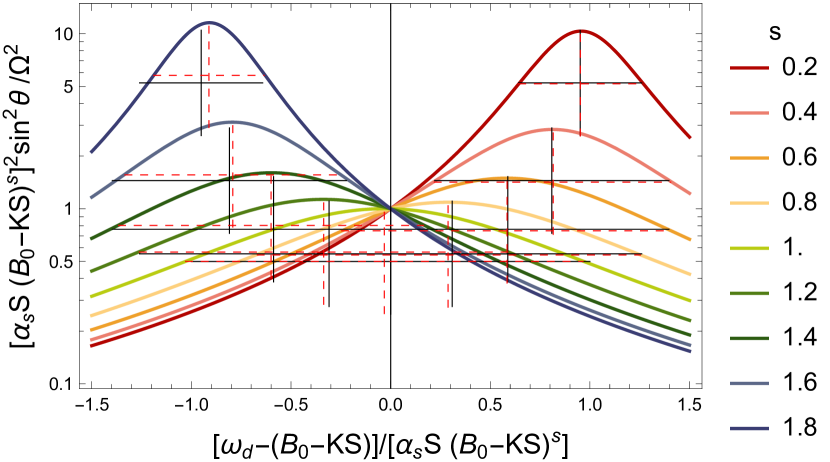
Figure 1: A lin-log plot of the amplitude $\sin^{2}\theta$ as a function of driving frequency $\omega_{d}$ plotted in dimensionless units for several values of $s$. The resonance peaks change, depending on $s$. The resonance frequency $\omega_{\text{res}}$ and linewidth $\Delta_{H/2}$ have been overlayed with crosses. The red dashed crosses have been calculated numerically, whereas the black solid crosses are the derived results from Eqs. (10) to (12).

Fractional Gilbert damping.— Fractional derivatives have a long history [29], and many different definitions exist for varying applications [29, 26, 27]. From our microscopic model, we found the Liouville derivative [41], which is defined as

$$D_{t}^{s}\bm{S}(t)=\frac{d^{n}}{dt^{n}}\frac{1}{\Gamma(n-s)}\int_{-\infty}^{t}dt^{\prime}(t-t^{\prime})^{n-1-s}\bm{S}(t^{\prime}),$$ (8)

where $n$ is the integer such that $n\leq s<n+1$. This can be interpreted as doing a fractional integral followed by an integer derivative. The fractional integral is a direct generalization from the rewriting of a repeated integral, by reversing the order of integration into a single one, which leads to extra powers of $(t-t^{\prime})$.

To provide some intuition to the effects of fractional friction, we propose a thought experiment. Suppose an object is traveling at constant speed, then $x(t)=vt$. Hence, the friction force acting on the object goes like $D_{t}^{s}x(t)\propto vt^{1-s}$. Therefore, we find three regimes. For $s=1$, the friction is constant in time. For $s<1$, the friction force increases with time. Hence, longer movements will be less common. For $s>1$, the friction decreases with time, so longer movements will be more likely once set in motion.

Within the fractional LLG equation, we thus see two important new regimes. For $s<1$ (sub-Ohmic), the friction is more likely to relax (localize) the spin (e.g. sub-diffusion) towards the $\bm{B}$-field direction. For small movements, the friction could be very small, whereas it would greatly increase for bigger movements. This could describe a low dissipation stable configuration. For $s>1$ (super-Ohmic), the friction could reduce as the spin moves further, which in other systems is known to cause Lévy-flights or super-diffusion [25, 24, 42]. This might lead the system to be less stable, but can potentially also greatly reduce the amount of dissipation for strong signal transfer: In a similar way to the design of fighter-jets, unstable systems can be easily changed by small inputs, which leads to more efficient signal transfer.

Ferromagnetic Resonance.— FMR is the phenomenon where the spin will follow a constant precession in a rotating external magnetic field. The angle $\theta$ from the $z$-axis at which it will do so in the steady state will vary according to the driving frequency $\omega_{d}$ of the magnetic field. Close to the natural frequency of the precession, one generally finds a resonance peak [43]. We assume a magnetic field of the form

$$\bm{B}_{\text{eff}}(t)=\begin{pmatrix}\Omega\cos(\omega_{d}t)\\ \Omega\sin(\omega_{d}t)\\ B_{0}-KS_{z}\end{pmatrix},$$ (9)

where $\Omega$ is the strength of the rotating component, and we will neglect thermal noise. We search for a steady state solution of $\bm{S}(t)$ in the rotating frame where $\bm{B}_{\text{eff}}(t)$ is constant. We will assume a small $\theta$ approximation where the ground state is in the positive $z$ direction, i.e. $0<\Omega\ll B_{0}-KS$ and $\alpha_{s}S\ll(B_{0}-KS)^{1-s}$. Then (see Sup. Mat. [36] for details of the calculations), we find that the resonance occurs at a driving frequency

$$\omega_{\text{res}}\approx(B_{0}-KS)+(B_{0}-KS)^{s}\alpha_{s}S\cos\left(\frac{\pi s}{2}\right).$$ (10)

It should be noted that this is different from what was to be expected from any scaling arguments, since the cosine term is completely new compared to previous results [43], and it vanishes precisely when $s=1$. However, this new non-linear term scales as $(B_{0}-KS)^{s}$, which is an easily controllable parameter. In the limit where $B_{0}-KS$ is small (resp. large), the linear term will vanish and the $s$-power scaling can be measured for the sub(resp. super)-Ohmic case. The amplitude at resonance is found to be

$$\sin^{2}\theta_{\text{res}}\approx\frac{\Omega^{2}}{\left[\alpha_{s}S(B_{0}-KS)^{s}\sin\left(\frac{\pi s}{2}\right)\right]^{2}},$$ (11)

and the Full Width at Half Maximum (FWHM) linewidth is given by

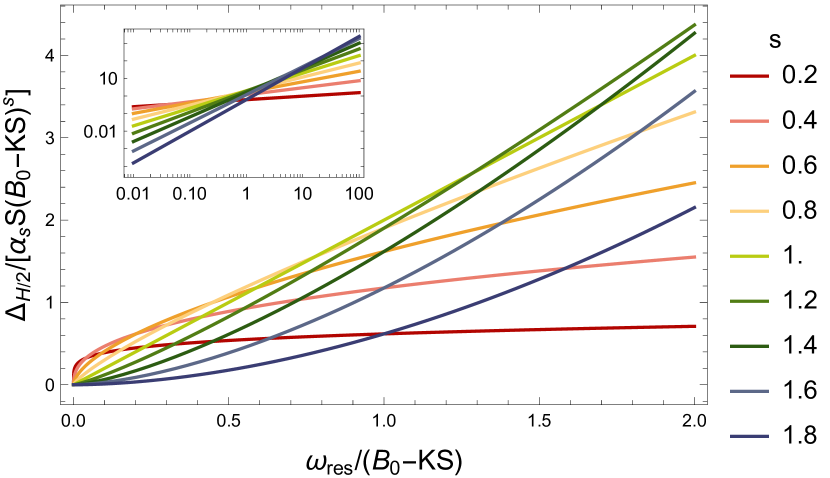
Figure 2: A plot of the linewidth in Eq. (13) as a function of resonance frequency for several values of $s$. The inset shows the same plot in a log-log scale, where the slope of the linewidth is precisely the Ohmicness $s$ of the bath.

$$\Delta_{H/2}\approx 2\alpha_{s}S(B_{0}-KS)^{s}\sin\left(\frac{\pi s}{2}\right).$$ (12)

Depending on the experimental setup, it might be easier to measure either the resonance location or the width of the peak. Nevertheless, both will give the opportunity to see the $s$ scaling in $B_{0}-KS$. The presence of the anisotropy provides a good opportunity to reach weak or strong field limits. In fact, the orientation of the anisotropy can help to add or subtract from the magnetic field, which should make the required field strengths more reachable for experiments. Some setups are more suitable for measuring the width as a function of resonance frequency. When $s=1$, this relation can be directly derived from Eqs. (10) and (12). However, when $s\neq 1$, the relation can only be approximated for strong or weak damping. For small $\alpha_{s}S$, we see that

$$\Delta_{H/2}\approx 2\alpha_{s}S(\omega_{\text{res}})^{s}\sin\left(\frac{\pi s}{2}\right).$$ (13)

The resonance peaks have been calculated numerically in FIG. 1 in dimensionless values. The red dashed lines show the location of the numerically calculated peak and the FWHM line width. The black solid lines show the location of the analytically approximated result for the peak location and FWHM line width [Eqs. (10) and (12)]. For small $\alpha_{s}S$ and $\Omega$, we see a good agreement between the analytical results and the numerical ones, although sub-Ohmic seems to match more closely than super-Ohmic. This could be due to the greater stability of sub-Ohmic systems, since the approximations might affect less a stable system. As one might expect from the thought experiment presented earlier, we can see in FIG. 1 that sub-Ohmic systems require higher, more energetic, driving frequencies to resonate, whereas super-Ohmic systems already resonate at lower, less energetic, driving frequencies. In FIG. 2, we provide a plot of Eq. (13) to facilitate further comparison with experiments. If the assumption of Gilbert damping was correct, all that one would see is a slope of one in the log-log inset.

Conclusion.— By relaxing the Ohmic Gilbert damping assumption, we have shown that the low-frequency regime of magnetization dynamics can be modeled by a fractional LLG equation. This was done by coupling the macrospin to a bath of harmonic oscillators in the framework of a Caldeira-Leggett model. The Keldysh formalism was used to compute the out-of-equilibrium dynamics of the spin system. By analyzing an FMR setup, we found an $s$-power scaling law in the resonance frequency and linewidth of the spin, which allows for a new way to measure the value of $s$. This means that experiments in magnetization dynamics and spintronics can now avoid the assumption of Gilbert damping and instead measure the Ohmicness of the environment. This could aid in a better understanding of how to improve efficiency, stability, and control of such systems for practical applications.

Acknowledgments.— This work was supported by the Netherlands Organization for Scientific Research (NWO, Grant No. 680.92.18.05, C.M.S. and R.C.V.) and (partly) (NWO, Grant No. 182.069, T.L. and R.A.D.).

References

- Mayergoyz et al. [2009] I. D. Mayergoyz, G. Bertotti, and C. Serpico, Nonlinear magnetization dynamics in nanosystems (Elsevier, 2009).
- Harder et al. [2016] M. Harder, Y. Gui, and C.-M. Hu, Physics Reports 661, 1 (2016).
- Barman et al. [2020] A. Barman, S. Mondal, S. Sahoo, and A. De, Journal of Applied Physics 128, 170901 (2020).
- Guo et al. [2021] Z. Guo, J. Yin, Y. Bai, D. Zhu, K. Shi, G. Wang, K. Cao, and W. Zhao, Proceedings of the IEEE 109 (2021).
- Lakshmanan [2011] M. Lakshmanan, Philosophical Transactions of the Royal Society A: Mathematical, Physical and Engineering Sciences 369, 1280 (2011).
- Awschalom and Flatté [2007] D. D. Awschalom and M. E. Flatté, Nature Physics 3, 153 (2007).
- Koopmans et al. [2005] B. Koopmans, J. J. M. Ruigrok, F. Dalla Longa, and W. J. M. de Jonge, Physical Review Letters 95, 267207 (2005).
- Duine et al. [2007] R. A. Duine, A. S. Núñez, J. Sinova, and A. H. MacDonald, Physical Review B 75, 214420 (2007).
- Caldeira and Leggett [1981] A. O. Caldeira and A. J. Leggett, Physical Review Letters 46, 211 (1981).
- Caldeira and Leggett [1983a] A. O. Caldeira and A. J. Leggett, Physica A: Statistical Mechanics and its Applications 121, 587 (1983a).
- Caldeira and Leggett [1983b] A. O. Caldeira and A. J. Leggett, Annals of Physics 149, 374 (1983b).
- Caldeira [2012] A. O. Caldeira, An introduction to macroscopic quantum phenomena and quantum dissipation, vol. 9780521113755 (Cambridge University Press, 2012).
- Weiss [2012] U. Weiss, Quantum dissipative systems (World scientific, 2012).
- Anders et al. [2022] J. Anders, C. R. Sait, and S. A. Horsley, New Journal of Physics 24, 033020 (2022).
- Groeblacher et al. [2015] S. Groeblacher, A. Trubarov, N. Prigge, G. Cole, M. Aspelmeyer, and J. Eisert, Nature communications 6, 1 (2015).
- Abdi and Plenio [2018] M. Abdi and M. B. Plenio, Physical Review A 98, 040303(R) (2018).
- Kehrein and Mielke [1996] S. K. Kehrein and A. Mielke, Physics Letters, Section A: General, Atomic and Solid State Physics 219, 313 (1996).
- Wilner et al. [2015] E. Y. Wilner, H. Wang, M. Thoss, and E. Rabani, Physical Review B - Condensed Matter and Materials Physics 92, 195143 (2015).
- Nalbach and Thorwart [2010] P. Nalbach and M. Thorwart, Physical Review B - Condensed Matter and Materials Physics 81, 054308 (2010).
- Paavola et al. [2009] J. Paavola, J. Piilo, K. A. Suominen, and S. Maniscalco, Physical Review A - Atomic, Molecular, and Optical Physics 79, 052120 (2009).
- Wu et al. [2013] N. Wu, L. Duan, X. Li, and Y. Zhao, Journal of Chemical Physics 138, 084111 (2013).
- Jeske et al. [2018] J. Jeske, A. Rivas, M. H. Ahmed, M. A. Martin-Delgado, and J. H. Cole, New Journal of Physics 20, 093017 (2018).
- Lemmer et al. [2018] A. Lemmer, C. Cormick, D. Tamascelli, T. Schaetz, S. F. Huelga, and M. B. Plenio, New Journal of Physics 20, 073002 (2018).
- Lutz [2012] E. Lutz, in Fractional Dynamics: Recent Advances (World Scientific, 2012), p. 285.
- Metzler and Klafter [2000] R. Metzler and J. Klafter, Physics Reports 339, 1 (2000).
- Mainardi [1997] F. Mainardi, Fractals and Fractional Calculus in Continuum Mechanics p. 291 (1997).
- De Oliveira and Tenreiro Machado [2014] E. C. De Oliveira and J. A. Tenreiro Machado, Mathematical Problems in Engineering 2014, 238459 (2014).
- Verstraten et al. [2021] R. C. Verstraten, R. F. Ozela, and C. Morais Smith, Physical Review B 103, L180301 (2021).
- Hilfer [2000] R. Hilfer, Applications of fractional calculus in physics (World scientific, 2000).
- Dalir and Bashour [2010] M. Dalir and M. Bashour, Applied Mathematical Sciences 4, 1021 (2010).
- Gardiner and Zoller [2004] C. Gardiner and P. Zoller, Quantum noise: a handbook of Markovian and non-Markovian quantum stochastic methods with applications to quantum optics (Springer Science & Business Media, 2004).
- Caldeira and Leggett [1985] A. O. Caldeira and A. J. Leggett, Phys. Rev. A 31, 1059 (1985).
- Kamenev [2011] A. Kamenev, Field theory of non-equilibrium systems (Cambridge University Press, 2011).
- Altland and Simons [2010] A. Altland and B. D. Simons, Condensed Matter Field Theory (Cambridge University Press, 2010), 2nd ed.
- Shnirman et al. [2015] A. Shnirman, Y. Gefen, A. Saha, I. S. Burmistrov, M. N. Kiselev, and A. Altland, Physical Review Letters 114, 176806 (2015).
- [36] R. C. Verstraten, T. Ludwig, R. A. Duine, and C. Morais Smith, Supplementary material.
- Kubo [1966] R. Kubo, Reports on Progress in Physics 29, 255 (1966).
- foo [a] In a straightforward variation with respect to quantum components, we would only obtain a noiseless quasi-classical equation of motion because the information about noise (fluctuations) is included in the Keldysh part of , which appears in the action only with even powers of quantum components. However, there is a way [44] that allows us to retain information about noise in the quasi-classical equation of motion; see also [34, 33]. Namely, we perform a Hubbard-Stratonovich transformation to linearize the contribution quadratic in quantum components. This linearization comes at the cost of introducing a new field, which takes the role of noise.
- foo [b] The dissipation kernel is closely related to the retarded and advanced components. Namely, it is given by .
- foo [c] From a mathematical perspective, any continuous but not smooth function can still be expanded in a power-law for small enough parameters. Hence, the only assumption that we make in this model is that the frequencies in the system are very small. Then, there will always exist an such that this expansion holds. In contrast, the Ohmic expansion can only be made for smooth continuous functions.
- foo [d] This definition does not have any boundary conditions, as they would have to be at and would dissipate before reaching a finite time. One can, however, enforce boundary conditions by applying a very strong magnetic field for some time such that the spin aligns itself, and then quickly change to the desired field at .
- Dubkov et al. [2008] A. A. Dubkov, B. Spagnolo, and V. V. Uchaikin, International Journal of Bifurcation and Chaos 18, 2649 (2008).
- Ludwig et al. [2020] T. Ludwig, I. S. Burmistrov, Y. Gefen, and A. Shnirman, Physical Review Research 2, 023221 (2020).
- Schmid [1982] A. Schmid, Journal of Low Temperature Physics 49, 609 (1982).