Good Data from Bad Models : Foundations of Threshold-based Auto-labeling

Abstract

Creating large-scale high-quality labeled datasets is a major bottleneck in supervised machine learning workflows. Auto-labeling systems are a promising way to reduce reliance on manual labeling for dataset construction. Threshold-based auto-labeling, where validation data obtained from humans is used to find a threshold for confidence above which the data is machine-labeled, is emerging as a popular solution used widely in practice [53, 45, 56]. Given the long shelf-life and diverse usage of the resulting datasets, understanding when the data obtained by such auto-labeling systems can be relied on is crucial. In this work, we analyze threshold-based auto-labeling systems and derive sample complexity bounds on the amount of human-labeled validation data required for guaranteeing the quality of machine-labeled data. Our results provide two insights. First, reasonable chunks of the unlabeled data can be automatically and accurately labeled by seemingly bad models. Second, a hidden downside of threshold-based auto-labeling systems is potentially prohibitive validation data usage. Together, these insights describe the promise and pitfalls of using such systems. We validate our theoretical guarantees with simulations and study the efficacy of threshold-based auto-labeling on real datasets.

1 Introduction

Machine learning models with millions or even billions of parameters are used to obtain state-of-the-art performance in various applications, e.g., object identification [47], machine translation [59], and fraud detection [66]. Such large-scale models require training on large-scale labeled datasets. As an outcome, the typical supervised machine learning workflow begins with construction of a large-scale high-quality dataset. Indeed, massive-scale labeled datasets, e.g., ImageNet [12], which have millions of labeled datapoints, have played a pivotal role in the advancement of computer vision. However, collecting labeled data is an expensive and time consuming process. A common approach is to rely on the services of crowd-sourcing platforms such as Amazon Mechanical Turk (AMT) to get ground-truth labels.

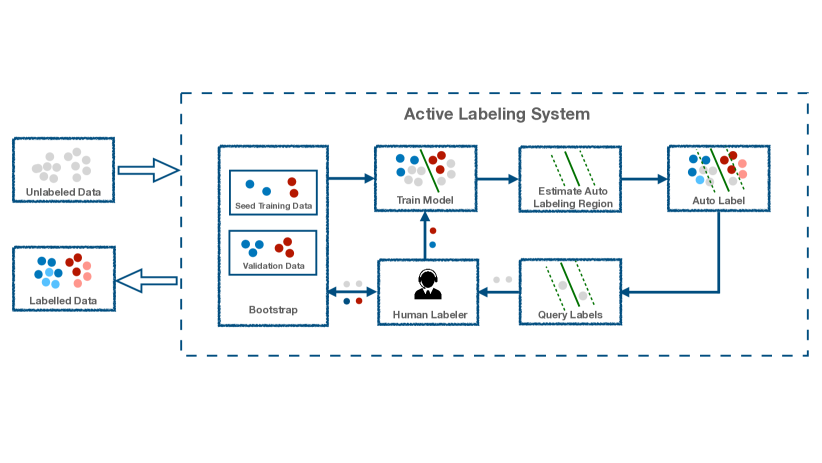
Figure 1: High Level Workflow of Threshold-Based Auto-Labeling Inspired from Industrial Auto-Labeling Systems.

Even when using crowd-sourcing, obtaining labels for all the points in the dataset remains slow and expensive. To reduce this cost, data labeling systems that partially rely on using a model’s predictions as labels have been developed. Such systems date back to teacher-less training [20]. Modern examples of these systems include Amazon Sagemaker Ground Truth [53] and others [50, 56, 1, 58]. These approaches to data labeling can be broadly termed auto-labeling.

An auto-labeling system tries to produce accurately labeled data using a given machine learning model while minimizing the cost of obtaining labels from humans. However, model outputs are often incorrect, leading to errors in datasets. The impact of these errors is further exacerbated due to the fact that the shelf life of datasets is longer than those of models. For example, ImageNet, which is a high-quality labeled dataset created mainly using human annotations, continues to be a benchmark for many computer vision tasks [12] fifteen years after its initial development. As a result, to reliably train new models on auto-labeled datasets and deploy them, we need a thorough understanding of how reliable the datasets output by these auto-labeling systems are.

Most of the widely used commercial auto-labeling systems [53, 56] are largely opaque with limited public information on their functionality. It is therefore unclear whether the quality of the datasets obtained can be trusted. To address this, we study the high-level workflow of a popular threshold-based auto-labeling system (see Figure 1). Such systems usually work iteratively. At a high level, in each iteration, the system trains a model on currently available human labeled data and decides to label certain parts of unlabeled data using the current trained model by finding high accuracy regions using validation data. It then collects human labels on a small portion of unlabeled data that is deemed helpful for training the current model in the next iteration. The validation data is created by sampling i.i.d. points from the unlabeled pool and querying human labels for them. In addition to the training data, the validation data is a major driver of the cost and accuracy of auto-labeling.

Our Contributions:

In this paper, we study threshold-based auto-labeling systems (Figure 1) and make the following contributions:

1. A theoretical characterization of threshold-based auto-labeling systems, developing tradeoffs between the quantity of manually-labeled training and validation data and the quantity and quality of auto-labeled data,

2. Findings indicating fundamental differences between active learning and auto-labeling,

3. Empirical results validating our theoretical understanding on real and synthetic data.

Our analysis establishes bounds on the quality (i.e., accuracy) and quantity (fraction of data) auto-labeled as a function of the validation data sample complexity and the training data sample complexity used in the auto-labeling procedure. These theoretical developments reveal two important insights. Promisingly, even poor-quality models are capable of reliably labeling at least some data when we have access to validation data and a good confidence function that can quantify the confidence of a given model on any data point. On the downside, in certain scenarios, the quantity of the validation data required to reach a certain quantity and quality of auto-labeled data can be high.

The rest of the paper is organized as follows. In Section 2, we provide a detailed description of threshold-based auto-labeling algorithm. In Section 3, we present and discuss the main results of our theoretical analysis. In Section 4, we present empirical results using both synthetic and real datasets. In Section 5 we discuss related literature and finally conclude in Section 6. Proofs and visualizations of auto-labeling are provided in the appendix in section 7.

2 Threshold-Based Auto-Labeling Algorithm

In this section, we discuss the threshold-based auto-labeling (TBAL) algorithm in detail. The high level workflow of the technique is shown in Figure 1. We begin by setting up notation before proceeding to describe the algorithm.

Notations

Let the instance space be $\mathcal{X}$ and the label space be $\mathcal{Y}=\{1,\ldots,k\}$. We assume that there is some deterministic but unknown function $f^{*}:\mathcal{X}\mapsto\mathcal{Y}$ that assigns label $y=f^{*}({\bf x})$ to any ${\bf x}\in\mathcal{X}$. We also assume that there is a noiseless oracle $\mathcal{O}$ that can provide the true label $y\in{\mathcal{Y}}$ for any given ${\bf x}\in\mathcal{X}$. Let $X_{pool}\subseteq\mathcal{X}$ denote a sufficiently large pool of unlabeled data that we must acquire labels for.

Given $X_{pool}\subseteq\mathcal{X}$, the goal of an auto-labeling algorithm is to produce labels $\tilde{y}_{i}\in\mathcal{Y}$ for points ${\bf x}_{i}\in X_{pool}$ while attempting to minimize the number of queries to the oracle. Let $[m]:=\{1,2,\ldots,m\}$. Let $A\subseteq[N]$ be the set of indices of auto-labeled points and let $X_{pool}(A)$ denote the corresponding set of points. The auto-labeling error denoted by $\widehat{\mathcal{E}}(X_{pool}(A))$ and the coverage denoted by $\widehat{\mathcal{P}}(X_{pool}(A))$ of the TBAL algorithm are defined as follows:

$$\widehat{\mathcal{E}}(X_{pool}(A))\vcentcolon=\frac{1}{N_{a}}\sum_{i\in A}\mathds{1}(\tilde{y}_{i}\neq f^{*}({\bf x}_{i})),$$ (1)

and

$$\widehat{\mathcal{P}}(X_{pool}(A))\vcentcolon=\frac{|A|}{N}=\frac{N_{a}}{N},$$ (2)

where $N_{a}$ denotes the size of auto-labeled set $A$. The goal of an auto-labeling algorithm is to auto-label the dataset so that $\widehat{\mathcal{E}}(X_{pool}(A))\leq\epsilon_{a}$ while maximizing coverage $\widehat{\mathcal{P}}(X_{pool}(A))$ for any given $\epsilon_{a}\in(0,1)$.

Hypothesis Class and Confidence Function:

A threshold-based auto-labeling algorithm is given a fixed hypothesis space $\mathcal{H}$ and a confidence function $g:\mathcal{H}\times\mathcal{X}\mapsto T\subseteq\mathbb{R}^{+}$ that quantifies the confidence of hypothesis $h\in\mathcal{H}$ on any on data point ${\bf x}\in\mathcal{X}$. Possible confidence functions include prediction probabilities and margin scores. For a concrete example, when $\mathcal{H}$ is set of unit norm homogeneous linear classifiers, i.e. $h_{{\bf w}}({\bf x})=\text{sign}({\bf w}^{T}{\bf x})$ with ${\bf w}\in\{{\bf w}\in\mathbb{R}^{d}:||{\bf w}||_{2}=1\}$, then a reasonable choice for the confidence function is $g(h_{{\bf w}},{\bf x})=|{\bf w}^{T}{\bf x}|$.

The algorithm proceeds iteratively. In each iteration, it queries for a subset of points which can be chosen actively using the information available so far and trains a classifier in $\mathcal{H}$ using the oracle-provided data. It then uses the confidence function and validation data to identify the region where the current classifier is confidently accurate and automatically labels the points in this region.

It is important to note that the target $f^{*}$ might not lie in the hypothesis space $\mathcal{H}$ that the auto-labeling algorithm works with. Our analysis (Section 3) shows that the auto-labeling algorithm can work well, i.e., accurately label a reasonable fraction of unlabeled data automatically, even with simpler hypothesis classes that do not contain the target hypothesis $f^{*}$. We illustrate this with a simple example in Section 2.1 and Figure 2.

The pseudo-code for the TBAL algorithm is given in Algorithm 1.

Algorithm 1 Threshold-based Auto-Labeling (TBAL) Algorithm

1:Unlabeled pool $X_{pool}$, Auto labeling error threshold $\epsilon_{a}$, Seed data size $n_{s}$, Batch size for active query $n_{b}$, Labeled validation data pool $D_{val}$.

2:$D_{out}=\{({\bf x}_{i},\tilde{y}_{i}):\forall{\bf x}_{i}\in X_{pool}\}$

3:$X_{u}^{(1)}=X_{pool}$

4:$D_{val}^{(1)}=D_{val}$

5:$D_{query}^{(1)}=\texttt{randomly\_query\_batch}(X_{u}^{(1)},n_{s})$

6:Remove queried points from $X_{u}^{(1)}$

7:$D^{(0)}_{train}=\phi;i=1$

8:$D_{out}=D_{out}^{(1)}=D_{query}^{(1)}$

9:while $X_{u}^{(i)}\neq\phi$ do

10:     $D^{(i)}_{train}=D^{(i-1)}_{train}\cup D^{(i)}_{query}$

11:     $\hat{h}_{i}=\texttt{empirical\_risk\_minimizer}(\mathcal{H},D_{train}^{(i)})$

12:     $\hat{t}_{i}=\text{Estimate Auto-labeling Threshold}(X_{u}^{(i)},\epsilon_{a},\hat{h}_{i},D_{val}^{(i)})$

13:     $D_{auto}^{(i)}=\{({\bf x},\hat{h}_{i}({\bf x})):{\bf x}\in X_{u}^{(i)},g(\hat{h}_{i},{\bf x})\geq\hat{t}_{i}\}$

14:     Remove auto-labeled points from $X_{u}^{(i)}$

15:     $D_{val}^{(i+1)}=D_{val}^{(i)}\setminus\{{\bf x}\in D_{val}^{(i)}:g(\hat{h}_{i},{\bf x})\geq\hat{t}_{i}\}$

16:     $D_{query}^{(i+1)}=\texttt{active\_query\_batch}(\hat{h}_{i},X_{u}^{(i)},n_{b})$

17:     Remove queried points from $X_{u}^{(i)}$

18:     $D_{out}=D_{out}\cup D_{auto}^{(i)}\cup D_{query}^{(i+1)}$

19:     $i=i+1$

Algorithm 2 Estimate Auto-Labeling Threshold

1:$X_{u}^{(i)},X_{v}^{(i)},\epsilon_{a},\hat{h}_{i},n_{0}$

2:Threshold $\hat{t}_{i}$

3:$\hat{T}_{i}=\{g(\hat{h}_{i},{\bf x}):\forall{\bf x}\in X_{u}^{(i)}\}$

4:$\hat{T}_{i}=\{t\in\hat{T}_{i}:|X_{v}^{(i)}(\hat{h}_{i},\hat{t}_{i})|\geq n_{0}\}\cup\{\infty\}$

5:$\hat{t}_{i}=\min\{t\in\hat{T}_{i}:\widehat{\mathcal{E}}_{a}(\hat{h}_{i},t|X_{v}^{(i)})+\hat{\sigma}(\hat{h}_{i},t,X_{v}^{(i)})\leq\epsilon_{a}\}$

Description of the algorithm: We are ready for a more detailed description of the algorithm. We start with an unlabeled pool of data points $X_{pool}$ and an auto-labeling error threshold $\epsilon$. For ease of exposition we let the algorithm be given labeled validation dataset $D_{val}$ of size $N_{v}$ separately. In practice, it is created by selecting points at random from the $X_{pool}$.

The algorithm starts with an initial batch of $n_{s}$ random data points and obtains oracle labels for these. The algorithm works in an iterative manner. The data obtained in each iteration $i$ is added to the training pool $D_{train}^{(i)}$. Next, the algorithm trains a model $\hat{h}_{i}$ by performing empirical risk minimization (ERM) on the training data $D_{train}^{(i)}$. In the next step, it proceeds to find the region where it can use $\hat{h}_{i}$ to auto-label accurately. To do so, the algorithm estimates a threshold score $\hat{t}_{i}$ above which it has the desired auto-labeling accuracy on the validation data (see Algorithm 2). Note that the errors on various thresholds are being estimated on the validation data. These estimates could be unreliable especially when the amount of validation data is small. Step 2 of this algorithm discards the thresholds that have a small amount of validation data. In step 3 we find the minimum threshold such that the sum of the estimated error and an upper confidence bound is at most the given auto-labeling error threshold. There can be various choices for $\hat{\sigma}$, such as, for example, the standard deviation of the estimated error $\widehat{\mathcal{E}}_{a}(\hat{h}_{i},t|X_{v}^{(i)})$. After getting the auto-labeling threshold $\hat{t}_{i}$ it proceeds to auto-label the points in $X_{u}^{(i)}$ and removes these auto-labeled points from the unlabeled pool. The validation points that fall in the auto-labeled region are also removed from the validation set so that in the next round the validation set and the unlabeled pool are from the same region and same distribution. If there are more unlabeled data points left in $X_{\text{pool}}$, the algorithm selects points using some active querying strategy, e.g., margin based active querying [2], and obtains human labels for them. This is added to the training pool for the next iteration. The same steps of training, auto-labeling and active querying are performed iteratively until there are no data points left to be labeled. In each round, the auto-labeled and human labeled data points are added to the set $D_{out}$ which is returned as output in the end. So, the dataset output by the TBAL algorithm has a mixture of human labeled and machine labeled data points.

 

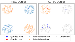
(a) Output of TBAL and AL+SC on XOR dataset

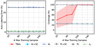
(b) Auto labeling performance of various methods

Figure 2: Comparison of Threshold-Based Auto-Labeling (TBAL) and Active-Learning followed by Selective Classification (AL+SC) on XOR-dataset. Left figure (a) shows samples that were auto-labeled, queried and left unlabeled by these methods. Right figure (b) shows the auto-labeling error and coverage achieved. The lines show the mean and the shaded region shows 1-standard deviation estimated over 10 trials with different random seeds.

2.1 Comparison between Auto-Labeling, Active Learning and Selective Classification

At the outset, a common question that can arise is what is the difference between TBAL (Algorithm 1) and methods such as active learning and selective classification. We address this question in this section.

Active learning.

Given a function class and an oracle that can label unlabeled data, the goal of active learning [51] is to find the best model in the function class by training with less labeled data compared to passive learning. This is usually achieved by an iterative approach wherein data to be labeled is carefully chosen so that it can be more informative given the observations so far. The end goal is to output a model from the function class that can do prediction on new data as well as the best model in the function class could.

Selective Classification.

Given a hypothesis class and a class of selection functions, the goal of selective classification [16] is to find the best combination of hypothesis function and selection function that minimizes the error in the predictions in the selected regions and maximizes the coverage of the selection region.

In contrast, the output of an auto-labeling procedure is a dataset. The final model is not necessarily of importance in this case. When the given function class is of lower complexity, it is often not possible to find a good classifier. The goal of an auto-labeling system is to still label as much of the unlabeled data as accurately as possible with a given function class and with limited labeled data from humans. The output dataset, which has a combination of labels obtained from humans and labels that were auto-labeled, is used to then train more complex models for a downstream task.

We contrast this difference between active learning, selective classification and auto-labeling through the following example. Consider using linear classifiers as function class for a dataset that is not linearly separable. We create a 2D synthetic dataset by uniformly drawing points from 4 circles, each centered at a corners of a square of with side length 4 centered at the origin. The points in the diagonally opposite balls belong to the same class, and hence we call it the XOR-dataset. We generate a total of $N=10,000$ samples, out of which we keep $8,000$ in $X_{pool}$ and $2,000$ in the validation pool ${X_{val}}$. We run the TBAL algorithm 1 with an error tolerance of $\epsilon_{a}=1\%$. We compare it with active learning and active learning followed by selective classification. The given function class and selective classifier are both linear for all the algorithms. The results are shown in in Figure 2. Clearly, there is no linear classifier that can correctly classify this data. We note that there are multiple optimal classifiers in the function class of linear classifiers and they will all incur an error of $25\%$. So, active learning algorithms can only output models that make at least $25\%$ error. If we naively use the output model for auto-labeling, we can obtain near full coverage but incur $25\%$ auto-labeling error. If we use the model output by active learning with threshold-based selective classification, then it can attain lower error in labeling. However, it can only label $\approx 25\%$ of the unlabeled data. In contrast, the TBAL algorithm is able to label almost all of the data accurately, i.e., attain close to $100\%$ coverage, with error close to $1\%$ auto-labeling error.

3 Theoretical Analysis

The performance of the TBAL algorithm 1 depends on the hypothesis class, the accuracy of the confidence function, the data sampling strategy, the size of the training data, and the size of the validation data. In particular, the size of the validation data plays a critical role in determining the accuracy of the confidence function which in turn affects the accuracy and coverage of automatically labeled data.

We derive bounds on the auto-labeling error and the coverage for Algorithm 1 in terms of the size of the validation data, the number of auto-labeled points $N_{a}^{(k)}$, and the Rademacher complexity of the extended hypothesis class $\mathcal{H}^{T,g}$ induced by the confidence function $g$. Our first result, Theorem (1), applies to general settings and makes no assumptions on the particular form of the hypothesis class, the data distribution, and the confidence function. We then instantiate and specialize the results for a specific setting in Section 3.1.

We introduce some notation to aid in stating our results,

Definition 1.

(Hypothesis Class with Abstain) Function $g$ (along with set $T$) induces an extended hypothesis class $\mathcal{H}^{T,g}$. Let $\mathcal{H}^{T,g}=\mathcal{H}\times T$. For any function $(h,t)\in\mathcal{H}^{T,g}$ is defined as

$$(h,t)({\bf x}):=\begin{cases}h({\bf x})&\quad\text{ if }g(h,{\bf x})\geq t\\ \perp&\quad\text{o.w.}\end{cases}$$ (3)

Here $(h,t)({\bf x})=\perp$ means the hypothesis $(h,t)$ abstains in classifying the point ${\bf x}$. Otherwise, it is equal to $h({\bf x})$. Let set $\mathcal{S}\subseteq\mathcal{X}$ denote a non-empty sub-region of $\mathcal{X}$ and $S\subseteq\mathcal{S}$ be a finite set of i.i.d. samples from $\mathcal{S}$. The subset $\mathcal{S}(h,t)\subseteq\mathcal{S}$ denotes the regions where $(h,t)$ does not abstain and the probability mass associated with it are

$$\mathcal{S}(h,t)\vcentcolon=\{{\bf x}\in\mathcal{S}:(h,t)({\bf x})\neq\perp\},\qquad\mathbb{P}(h,t|\mathcal{S})\vcentcolon=\mathbb{P}(\mathcal{S}(h,t)|\mathcal{S}),\qquad\widehat{\mathbb{P}}(h,t|S)\vcentcolon=\frac{|S(h,t)|}{|S|}.$$

In general we use $\mathbb{P}(\mathcal{S})$ to denote the probability mass of set $\mathcal{S}$ and $\mathbb{P}(\mathcal{S}^{\prime}|\mathcal{S})$ for the conditional probability of subset $\mathcal{S}^{\prime}\subseteq\mathcal{S}$ given $\mathcal{S}$. Their empirical counterparts are denoted as $\widehat{\mathbb{P}}(S)$ and $\widehat{\mathbb{P}}(S^{\prime}|S)$ respectively.

Loss Functions: We use the following loss functions,

$$\ell_{0-1}(h,{\bf x},y) \vcentcolon=\mathds{1}(h({\bf x})\neq y),\quad\ell_{\perp}(h,t,{\bf x})\vcentcolon=\mathds{1}(g(h,{\bf x})\geq t),\quad\ell_{0-1}^{\perp}(h,t,{\bf x},y) \vcentcolon=\ell_{0-1}(h,{\bf x},y)\cdot\ell_{\perp}(h,t,{\bf x}).$$

Error Definitions: Define the conditional error in set $\mathcal{S}\subseteq\mathcal{X}$ denoted by $\mathcal{E}(h,t|\mathcal{S})$ and the conditional error in set $\mathcal{S}(h,t)$ i.e. the subset of $\mathcal{S}$ on which $(h,t)$ does not abstain denoted by $\mathcal{E}(h,t|\mathcal{S}(h,t))$ as follows:

$$\mathcal{E}(h,t|\mathcal{S})\vcentcolon=\mathbb{E}_{{\bf x}|\mathcal{S}}[\ell_{0-1}^{\perp}(h,t,{\bf x},y)]\qquad\text{and}\qquad\mathcal{E}_{a}(h,t|\mathcal{S})\vcentcolon=\mathcal{E}(h,t|\mathcal{S}(h,t))=\frac{\mathcal{E}(h,t|\mathcal{S})}{\mathbb{P}(h,t|\mathcal{S})}.$$

Similarly, define their empirical counterparts as follows,

$$\widehat{\mathcal{E}}(h,t|S)\vcentcolon=\frac{1}{|S|}\sum_{{\bf x}_{i}\in S}\ell_{0-1}^{\perp}(h,t,{\bf x}_{i},y_{i}),\qquad\widehat{\mathcal{E}}_{a}(h,t|S)\vcentcolon=\widehat{\mathcal{E}}(h,t|S(h,t))\vcentcolon=\frac{1}{|S(h,t)|}\sum_{{\bf x}_{i}\in S(h,t)}\ell_{0-1}^{\perp}(h,t,{\bf x}_{i},y_{i}),$$

In this notation, the auto-labeling error in $i$-th epoch is given by, $\widehat{\mathcal{E}}_{a}(\hat{h}_{i},\hat{t}_{i}|X_{u}^{(i)})=m_{a}^{(i)}/n_{a}^{(i)}$ where $m_{a}^{(i)}=\sum_{{\bf x}_{j}\in X_{u}^{(i)}(\hat{h}_{i},\hat{t}_{i})}\ell_{0-1}^{\perp}(\hat{h}_{i},\hat{t}_{i},{\bf x}_{j},y_{j})$ is the number of auto-labeling mistakes in $i$-th epoch and $n_{a}^{(i)}=|X_{u}^{(i)}(\hat{h}_{i},\hat{t}_{i})|$ is the number of auto-labeled points in that epoch.

Rademacher Complexity: The Rademacher complexities for the function classes induced by the $\mathcal{H},T,g$ and the loss functions are defined as follows:

$$\mathfrak{R}_{n}\big{(}\mathcal{H}^{T,g}\big{)}\vcentcolon=\mathfrak{R}_{n}\big{(}\mathcal{H},\ell_{0-1}\big{)}+\mathfrak{R}_{n}\big{(}\mathcal{H}^{T,g},\ell_{\perp}\big{)}$$ (4)

Let $\hat{h}_{i}$ and $\hat{t}_{i}$ be the ERM solution and the auto-labeling threshold, respectively, at epoch $i$. Let $p_{\!{}_{0}}\in(0,1)$ be a constant such that $\mathbb{P}(\hat{h}_{i},\hat{t}_{i}|\mathcal{X}^{(i)})\geq p_{\!{}_{0}},\ \forall i$. Also let $X_{v}^{(i)}$ denote the validation set, $n_{v}^{(i)}$ and $n_{a}^{(i)}$ denote the number of validation and auto-labeled points at epoch $i$. Let $\widehat{\mathcal{E}}_{a}(\hat{h}_{i},\hat{t}_{i}|X_{v}^{(i)})$ denote the empirical conditional risk of $\hat{h}_{i}$ in the region where $g(\hat{h}_{i},{\bf x})\geq\hat{t}_{i}$ evaluated on the validation data $X_{v}^{(i)}$.

The following theorem provides guarantees on the auto-labeling error and the coverage achieved by the TBAL algorithm.

[]theoremgeneralTheoremMain (Overall Auto-Labeling Error and Coverage) Let $k$ denote the number of rounds of the TBAL Algorithm 1. Let $n_{v}^{(i)},n_{a}^{(i)}$ denote the number of validation and auto-labeled points at epoch $i$ and $n^{(i)}=|X^{(i)}|$. Let $X_{pool}(A_{k})$ be the set of auto-labeled points at the end of round $k$. $N_{a}^{(k)}=\sum_{i=1}^{k}n_{a}^{(i)}$ denote the total number of auto-labled points. Then, with probability at least $1-\delta/2$,

$$\widehat{\mathcal{E}}\Big{(}X_{pool}(A_{k})\Big{)} \leq\sum_{i=1}^{k}\frac{n_{a}^{(i)}}{N_{a}^{(k)}}\Bigg{(}\underbrace{\widehat{\mathcal{E}}_{a}\Big{(}\hat{h}_{i},\hat{t}_{i}|X_{v}^{(i)}}_{(a)}\Big{)}+\frac{4}{p_{\!{}_{0}}}\big{(}\underbrace{\mathfrak{R}_{n_{v}^{(i)}}\big{(}\mathcal{H}^{T,g}\big{)}+\frac{2}{p_{\!{}_{0}}}\sqrt{\frac{1}{n_{v}^{(i)}}\log(\frac{8k}{\delta})}}_{(b)}\Bigg{)}$$

$$+\frac{4}{p_{\!{}_{0}}}\Bigg{(}\underbrace{\sum_{i=1}^{k}\frac{n_{a}^{(i)}}{N_{a}^{(k)}}\mathfrak{R}_{n_{a}^{(i)}}\big{(}\mathcal{H}^{T,g}\big{)}+\sqrt{\frac{k}{N_{a}^{(k)}}\log(\frac{8k}{\delta})}}_{(c)}\Bigg{)}$$

and w.p. at least $1-\delta/2$

$$\widehat{\mathcal{P}}({X_{pool}(A_{k})})\geq\sum_{i=1}^{k}\mathbb{P}\big{(}\mathcal{X}^{(i)}(\hat{h}_{i},\hat{t}_{i})\big{)}-2\mathfrak{R}_{n^{(i)}}\big{(}\mathcal{H}^{T,g}\big{)}-\sqrt{\frac{2k^{2}}{N}\log\Big{(}\frac{8k}{\delta}\Big{)}}.$$

Discussion. We interpret this result, starting with the auto-labeling error term $\widehat{\mathcal{E}}(X_{pool}(A_{k})).$ The term (a) $\widehat{\mathcal{E}}_{a}(\hat{h}_{i},\hat{t}_{i}|X_{v}^{(i)})$ is the empirical conditional error in the auto-labeled region computed on the validation data in $i$-th round, which is at most $\epsilon_{a}$. Thus, summing term (a) over all the rounds is at most $\epsilon_{a}$. The term (b) provides an upper bound on the excess error over the empirical estimate term (a) as a function of the Rademacher complexity of $\mathcal{H}^{T,g}$ and the validation data used in each round. The last term (c) captures the variance in the overall estimate as function of the total number of auto-labeled points and the Rademacher complexity of $\mathcal{H}^{T,g}$. If we let $n_{v}^{(i)}\geq n_{v}$ i.e. the minimum validation points ensured in each round, then we can see the second term is $\mathcal{O}(\mathfrak{R}_{n_{v}}(\mathcal{H}^{T,g}))$ and the third term is $\mathcal{O}\left(\sqrt{\frac{1}{n_{v}}}\right)$. Therefore, validation data of size $\mathcal{O}\left(\frac{1}{\epsilon_{a}^{2}}\right)$ in each round is sufficient to get a $\mathcal{O}(\epsilon_{a})$ bound on the excess auto-labeling error. The terms with Rademacher complexities suggest that it is better to use a hypothesis class and confidence function such that the induced hypothesis class has low Rademacher complexity. While such a hypothesis class might not be rich enough to include the target function, it would still be helpful for efficient and accurate auto-labeling of the dataset which can then be used for training richer models in the downstream task. The coverage term provides a lower bound on the empricial coverage $\widehat{\mathcal{P}}({X_{pool}(A_{k})})$ in terms of the true coverage of the sequence of estimated hypothesis $\hat{h}_{i}$ and threshold $\hat{t}_{i}$.

We note that the size of the validation data needed to guarantee the auto-labeling error in each round by Algorithm 1 is optimal up to $\log$ factors. This follows by applying the result on the tail probability of sum of independent random variables due to Feller [19]: []lemmalowerBound Let $c_{1},c_{2}$ and $\sigma>0$. Let ${\bf x}_{i}\in X$ be a set of $n$ i.i.d. points from $\mathcal{X}$ with corresponding true labels $y_{i}$. Given $(h,t)\in\mathcal{H}^{T,g}$, let $\mathbb{E}\big{[}\big{(}\ell_{0-1}^{\perp}(h,t,{\bf x}_{i},y_{i})-\mathcal{E}(h,t|\mathcal{X})\big{)}^{2}\big{]}=\sigma_{i}^{2}>\sigma^{2}$ for every ${\bf x}_{i}$ for $\sigma_{i}>0$ and let $\sum_{i}^{n}\sigma_{i}^{2}\geq c_{1}$ then for every $\epsilon\in[0,\frac{\sum_{i=1}^{n}\sigma_{i}^{2}}{\sqrt{c_{1}}}]$ with $n_{v}<\frac{12\sigma^{2}}{\epsilon^{2}}\log(4c_{2})$ the following holds w.p. at least $1/4$, $\mathcal{E}_{a}(h,t|\mathcal{X})>\widehat{\mathcal{E}}_{a}(h,t|X)+\epsilon.$ Therefore, if a sufficiently large validation set is not used in each round, there is a constant probability of erroneously deciding on a threshold for auto-labeling. We further note that such a requirement on validation data also applies to active learning if we seek to validate the output model. Bypassing this requirement demands the use of approaches that are different from threshold-based auto-labeling and traditional validation techniques. We note the possibility of using recently-proposed active testing techniques [31], a nascent approach to reducing validation data usage.

3.1 Linear Classifier Setting

Next we instantiate the results in Theorem 1 for the case of homogeneous linear separators under the uniform distribution in the realizable setting. Formally, let $P_{\bf x}$ be supported on the unit ball in $\mathbb{R}^{d}$, $\mathcal{X}=\{{\bf x}\in\mathbb{R}^{d}:||{\bf x}||\leq 1\}$. Let $\mathcal{W}=\{{\bf w}\in\mathbb{R}^{d}:||{\bf w}||_{2}=1\}=\mathbb{S}_{d}$, $\mathcal{H}=\{{\bf x}\mapsto\text{sign}(\langle{\bf w},{\bf x}\rangle)\,\forall{\bf w}\in\mathcal{W}\}$, the score function be given by $g(h,{\bf x})=g({\bf w},{\bf x})=|\langle{\bf w},{\bf x}\rangle|$, and set $T=[0,1]$. For simplicity we will use $\mathcal{W}$ in place of $\mathcal{H}$.

[]corollarylinearMainTheorem (Overall Auto-Labeling Error and Coverage) Let $\hat{{\bf w}}_{i},\hat{t}_{i}$ be the ERM solution and the auto-labeling margin threshold respectively at epoch $i$. Let $n_{v}^{(i)},n_{a}^{(i)}$ denote the number of validation and auto-labeled points at epoch $i$. Let the auto-labeling algorithm run for $k$-epochs. Then, w.p. at least $1-\delta/2$,

$$\widehat{\mathcal{E}}(X_{pool}(A_{k})) \leq\sum_{i=1}^{k}\frac{n_{a}^{(i)}}{N_{a}^{(k)}}\Bigg{(}\underbrace{\widehat{\mathcal{E}}_{a}(\hat{{\bf w}}_{i},\hat{t}_{i}|X_{v}^{(i)})}_{(a)}+\underbrace{\frac{4}{p_{\!{}_{0}}}\sqrt{\frac{2}{n_{v}^{(i)}}\bigg{(}2d\log\Big{(}\frac{en_{v}^{(i)}}{d}\bigg{)}+\log\Big{(}\frac{8k}{\delta}\bigg{)}\bigg{)}}\Bigg{)}}_{(b)}$$

$$+\underbrace{\frac{4}{p_{\!{}_{0}}}\Bigg{(}\sqrt{\frac{2k}{N_{a}^{(k)}}\bigg{(}2d\log\Big{(}\frac{eN_{a}^{(k)}}{d}\bigg{)}+\log\Big{(}\frac{8k}{\delta}\bigg{)}\bigg{)}}\Bigg{)}}_{c}$$

and w.p. at least $1-\delta/2$

$$\widehat{\mathcal{P}}(X_{pool}(A_{k}))\geq 1-\min_{i}\hat{t}_{i}\sqrt{4d/\pi}-2k\sqrt{\frac{2}{N}\bigg{(}2d\log\Big{(}\frac{eN}{d}\Big{)}+\log\Big{(}\frac{8k}{\delta}\Big{)}\bigg{)}}.$$

By applying standard VC theory to the first round, we obtain that $\hat{t}_{1}\leq 1/2$. Therefore, right after the first round, we are guaranteed to label at least half of the unlabeled pool. We empirically observe that TBAL has coverage at par with active learning while respecting the auto-labeling error constraint (See Figure 3(a).

The details of the proofs of the results presented in this section are found in the appendix.

 

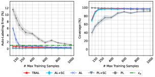
(a) Performance with varying training data size. Validation size used here is 4000.

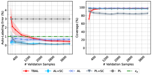
(b) Performance with varying validation data size. Max training samples = 500.

Figure 3: Auto-labeling performance on the Unit-Ball dataset. Left figure (a) We keep validation data size same for all methods and vary the training data size. In the right figure (b) we keep the training data size fixed and vary the validation data size. The auto-labeling error threshold $\epsilon_{a}=1\%$ in both experiments. The lines show the mean and the shaded region shows 1-standard deviation estimated over 10 trials with different random seeds.

4 Experiments

We study the effectiveness of threshold based auto-labeling (TBAL) on synthetic and real datasets. Our goal is to validate our theoretical results and understand the amount of labeled validation and training data required by the algorithm to achieve a certain auto-labeling error and coverage. We also seek to understand whether our findings apply to real data—where labels may be noisy—along with how well TBAL performs compared to common baselines.

Baselines

We compare TBAL to the following methods that can be used to create auto-labeled datasets,

• Passive Learning (PL): This method queries a subset of the points randomly to train a model from a given model class and then uses it to predict the labels for the remaining unlabeled pool.

• Active Learning (AL): This method uses active learning (using margin-random query strategy which is described below) to train a model from a given model class and then uses it to predict the labels for the remaining unlabeled pool.

• Passive Labeling + Selective Classification (PL+SC) This method first performs passive learning to train a model from a given model class. Then it performs auto-labeling on the unlabeled using threshold-based selective classification with the model output by passive learning. So, only those unlabeled points that are deemed as fit to be labeled by the selection function are auto-labeled.

• Active Learning + Selective Classification (AL+SC): This method first performs active learning (using margin-random query strategy which is described below) to train a model from a given model class. Then it performs auto-labeling using threshold-based selective classification with the model output by active learning.

For selective classification in the above methods we use the same Algorithm 2 to estimate threshold and perform auto-labeling using the estimated threshold. In experiments, we adapt Algorithm 2 slightly—instead of estimating a single threshold for all classes, we estimate thresholds for each class separately.

   

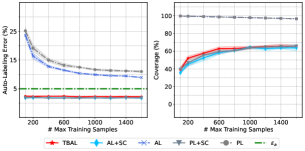
(a) Auto-labeling MNIST data using linear classifier. Validation size used here is 12k.

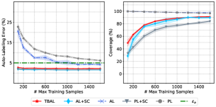
(b) Auto-labeling MNIST data using LeNet classifier. Validation size used her is 12k.

Figure 4: Auto-labeling performance on MNIST data using different models (hypothesis classes) as a function of samples available for training. Left figure (a) shows the results with linear classifier and the right figure (b) shows the results with LeNet classifier. The auto-labeling error threshold $\epsilon_{a}=5\%$ in both experiments and the algorithms are given same amount of validation data. The lines show the mean and the shaded region shows 1-standard deviation estimated over 5 trials with different random seeds.

Active Querying Strategy

We use the margin-random query strategy for querying the next batch of training data. In this strategy, the algorithm first sorts the points based on the margin score and then selects the top $Cn_{b}$ ($C>1$) points from which $n_{b}$ points are picked at random. This is a simple and computationally efficient method that balances the exploration and exploitation trade-off. We note that other active-querying strategies exist; we use margin-random as our standard querying strategy to keep the focus on comparing auto-labeling—not active learning approaches.

Datasets

We use four datasets, two synthetic and two real. For each dataset we split the data into two sufficiently large pools. One is used as $X_{pool}$ on which auto-labeling algorithms are run and the other is used as $X_{val}$ from which the algorithms subsample validation data. The datasets are

• Unit-Ball is a synthetic dataset where $\mathcal{X}$ is the $d$-dimensional unit ball and points are selected uniformly from it. The true labels are generated using a homogeneous linear separator with ${\bf w}=[1/\sqrt{d},\ldots,1/\sqrt{d}]$. We use $d=30$ and generate $N=20,000$ samples, out which we keep $16,000$ in $X_{pool}$ and create a validation pool $X_{val}$ of size $4,000$.

• XOR is a synthetic dataset. Recall that it is created by uniformly drawing points from 4 circles, each centered at a corners of a square of with side length 4 centered at origin. Points in the diagonally opposite balls belong to the same class. We generate a total of $N=10,000$ samples, out of which we keep $5,000$ in $X_{pool}$ and $5,000$ in the validation pool ${X_{val}}$.

• MNIST [13] is a standard image dataset of hand-written digits. We randomly split the standard training set into $X_{pool}$ and the validation pool $X_{val}$ of sizes 48,000 and 12,000 respectively . While training a linear classifier on this dataset we flatten the $28\times 28$ images to vectors of size 784.

• CIFAR-10 [32] is a image dataset of 10 classes. We randomly split the standard training set into $X_{pool}$ of size 40,000 and the validation pool $X_{val}$ of size 10,000.

Models and Training: For the linear models we use SVM with the usual hinge loss and train it till loss tolerance 1e-5. For training LeNet [35] we use SGD with learning rate 0.1, batch size 32 and train for 20 epochs.

With SVM classifiers we use standard implementations of [64, 42] in sklearn library to get the prediction probabilities and use them as the score function. For neural networks we use softmax output and [36] as the score functions.

4.1 Role of Validation Data

We first study the role of validation data in the auto-labeling performance of the methods. As the validation data plays a crucial role in determining the threshold for automatically labeling unlabeled points with confidence, we expect that the accuracy of auto-labeled points will decrease with smaller validation data.

Setup

We use the Unit-Ball dataset with a homogeneous linear separator being the true function. We keep the maximum training data size $N_{q}$ fixed at 500 and vary the validation data size given to the algorithms. Since this is a linearly separable setting with linear classifier as the function class for the models being trained, we set the auto-labeling error threshold $\epsilon_{a}$ to be $1\%$. We give initial seed data of size $n_{s}$ is 20% of $N_{q}$ and use a query batch size $n_{b}$ is $5\%$ of $N_{q}$ and $C=2$ for both AL and TBAL . We give the same initial seed samples of size $n_{s}$ to all the methods to ensure they get the same starting point.

Results

Figure 3(b) shows the auto-labeling error and the coverage achieved by TBAL and other algorithms. As expected, if the validation data provided to the TBAL algorithm is insufficient, resulting auto-labeling error is higher as it starts to auto-label from initial rounds unlike other baselines which auto-label only in the end. We observe that the auto-labeling error as well as the coverage of the TBAL algorithm improves as more validation data is used. This is also highlighted by our theoretical analysis (see Theorem 1).

4.2 Role of Hypothesis Class

An important consideration is the choice of the function class used to perform auto-labeling. In practice one does not know the true function class. Choosing a powerful function class such as deep neural networks requires large amounts of labeled training samples which defeats the purpose of creating an auto-labeled dataset for future training purposes. Here we examine whether in less powerful hypothesis classes—in particular, where the best classifier in the class has a constant risk—it is possible to auto-label the data with high accuracy and reasonably large coverage.

Setup

We study this question by performing auto-labeling using linear classifiers in the settings where the data is not linearly separable. We first study this on the synthetically generated XOR dataset. We then run the experiment on the MNIST dataset. For both datasets we use 20% of $N_{q}$ as seed training data and keep query size $n_{b}$ as $5\%$ of $N_{q}$. The auto-labeling error threshold given in these settings are $1\%$ and $5\%$ for XOR and MNIST respectively.

Results

The results for XOR are depicted in Figure 2(b) and on MNIST are shown in Figure 4(a).

In the XOR setting we find that TBAL can auto-label almost all the data accurately. Even though the Bayes risk of the linear classifier model for this setting is 25%, TBAL can still provide a good dataset with great coverage. In contrast, other methods that auto-label using the final model are limited either to 25% accuracy or at most 25% coverage.

We study the same question in the real data setting (Figure 4 ) and observe that TBAL using less powerful models can still yield highly accurate datasets with a significant fraction of points labeled by the models. This confirms the notion that bad models can still provide good datasets.

4.3 Role of Training Data Size

The labels queried as a part of model training also play an important role and incur cost in the process. Our next experiment focuses on the impact of training data on auto-labeling.

Setup

We limit the amount of training data the algorithm can use and observe the auto-labeling error and coverage. We ensure all the algorithms have sufficiently large but equal amount of validation data. We run this experiment on the Unit-Ball, XOR, and MNIST datasets. We use the same values of $n_{s}$ and $n_{b}$ and $C$ as previous experiments.

Results The results are shown in Figures 2(b),3(a), and 4. We observe that the auto-labeling error of TBAL and methods based on selective classification (AL+SC, PL+SC) is close to or lower than the given auto-labeling error threshold, even in the low training samples regime. The coverage is low when given fewer samples for training, which is expected since they cannot get to a higher accuracy model with fewer samples and therefore the regions that can be confidently auto-labeled will be smaller. However, with more training samples they are expected to learn a good model within the function class and thus their coverage improves.

4.4 Role of Confidence Function

The confidence function $g$ is used to obtain uncertainty scores is an important factor in auto-labeling. In particular, for threshold based auto-labeling we expect the scores of correctly classified and incorrectly classified points to be reasonably well separated and if this is not the case then the algorithm will struggle to find a good threshold even the given classifier has good accuracy in certain regions.

Setup We perform auto-labeling on CIFAR-10 dataset using a small CNN network with 2 convolution layers followed by 3 fully connected layers  [43]. We use two different scores for auto-labeling, a) Usual softmax output b) Energy score with temperature = 1 [36]. We vary the maximum number of training samples $N_{q}$ and keep 20% of $N_{q}$ as seed samples and query points in the batches of $10\%$ of $N_{q}$. The model is trained for 50 epochs, using SGD with learning rate 0.05, batch size = 256, weight decay = $5e^{-4}$ and momentum=0.9. The auto-labeling threshold is set to 10%.

Results The results with softmax scores and energy scores used as confidence functions can be seen in Figures 6(a) and 6(b) respectively. We see that for both of these cases, TBAL does not obtain a coverage of more that $\approx 6\%$. We observe that using energy score as the confidence function performed marginally better than using the softmax scores. We note that this is the case even though the test accuracies of the trained models were around $50\%$ for most of the rounds. Note that CIFAR-10 has 10 classes, so accuracy of $50\%$ is much better than random guessing and one would expect to be able to auto-label a significant chunk of the data with such a model. However, the softmax scores and energy scores are not well calibrated and therefore, when used as confidence functions, they result in poor separation between correct and incorrect predictions by the model. This can be seen in Figure 6 where neither of the softmax and energy scores provide a good separation between the correct and incorrect predictions. We can also see that the energy score is marginally better in terms of the separation, which allows it to achieve a slightly better auto-labeling coverage in comparison to using softmax scores. This suggests that more investigation is needed to understand the properties of good confidence functions for auto-labeling which is left to future work. For more detailed visualization of the rounds of TBAL for this experiment, see Figures 8 and 9 in the Appendix.

 

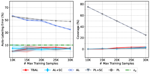
(a) Auto-labeling CIFAR-10 data using a small network and softmax scores. Validation size = 10k .

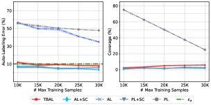
(b) Auto-labeling CIFAR-10 data using a small network and energy scores. Validation size = 10k .

Figure 5: Auto-labeling performance on CIFAR-10 data using a small network and different scoring functions. Left figure (a) shows the results with softmax scores and the right figure (b) shows the results with the energy score. The auto-labeling error threshold $\epsilon_{a}=10\%$ in both experiments and algorithms are given same amount of validation data. The lines show the mean and the shaded region shows 1-standard deviation estimated over 5 trials with different random seeds.

 

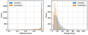
(a) Histogram of scores in round 2.

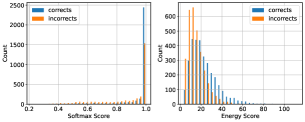
(b) Histogram of scores in round 6.

Figure 6: Histograms of scores computed on the validation data in a few rounds of TBAL run on CIFAR-10 with small net. We picked two rounds where it auto-labeled the most i.e. around 800 points.

5 Related Work

We briefly review the related literature in this section.

There is a rich body of work on active learning on empirical and theoretical fronts  [51, 11, 28, 27, 6, 49]. In active learning the goal is to learn the best model in the given function class with fewer labeled data than the classical passive learning. To this end, various active learning algorithms have been developed and analyzed, e.g., uncertainty sampling [57, 40] , disagreement region based [5, 26], margin based [2, 4], importance sampling based [3] and others [9]. Active learning has been shown to achieve exponentially smaller label complexity than passive learning in noiseless and low-noise settings [14, 2, 26, 27, 4, 10, 28, 9, 30, 33]. This suggests, in these settings auto-labeling using active learning followed by selective classification is expected to work well. However in practice we do not have the favorable noise conditions and the hypothesis class could be misspecified i.e. it may not contain the Bayes optimal classifier. In such cases [29] proved lower bounds on the label complexity of active learning that are order wise same as passive learning. These findings have motivated more refined goals for active learning – abstain on hard to classify points and do well on the rest of the points. This idea is captured by the Chow’s excess risk [8] and some of the recent works  [52, 55, 44, 65] have proved exponential savings in label complexity for active learning when the goal is to minimize Chow’s excess risk. The classifier learned by these methods is equipped with the abstain option and hence it can be readily applied for auto-labeling. However, the problem of mis-specification of the hypothesis class still remains. Nevertheless, it would be an interesting future work to explore the connections between auto-labeling and active learning with abstention. We also note that similar works on learning with abstention are done in the context of passive learning  [7].

Another closely related line of work is selective classification where the goal is to equip a given classifier with the option to abstain from prediction in order to guarantee prediction quality. The foundations for selective classification are laid down in [16, 60, 17, 61] where they give results on the error rate in the prediction region and the coverage of a given classifier. However, they lack practical algorithms to find the prediction region. A recent work [23] proposes a new disagreement based active learning strategy to learn a selective classifier.

A recent work studies a practical algorithm for threshold based selective classification on deep neural networks [22]. The algorithm estimates prediction threshold using training samples and they bound error rate of the selective classifier using [21]. We note that their result is applicable to a specific setting of a given classifier. In contrast, in the TBAL algorithm analyzed in this paper, selective classification is done in each round and the classifiers are not given a priori but instead learned via ERM on training data which is adaptively sampled in each round.

Another related work [45] studies algorithm similar to TBAL for auto-labeling. Their emphasis is on the cost of training incurred when these systems use large scale model classes for auto-labeling. They propose an algorithm to predict the training set size that minimizes the overall cost and provide an empirical evaluation.

Well calibrated uncertainty scores are essential to the success of threshold based auto-labeling. However, in practice such scores are often hard to get. Moreover, neural networks can produce overconfident ( unreliable) scores [25]. Fortunately, there are plenty of methods in the literature to deal with this problem [42, 64]. More recently, various approaches have been proposed for uncertainty calibration for neural networks [24, 38, 62, 34, 39, 54]. A detailed study of calibration methods and their impact on auto-labeling is beyond the scope of this work and left as future work.

There is another line of work emerging towards auto-labeling that does not rely on getting human labels but instead uses potentially noisy but cheaply available sources to infer labels [48, 46, 18]. The focus of this paper, however, is on analyzing the performance of TBAL algorithms [53, 1] that have emerged recently as auto-labeling solutions in systems.

6 Conclusion and Future Works

In this work, we analyzed threshold-based auto-labeling systems and derived sample complexity bounds on the amount of human-labeled validation data required for guaranteeing the quality of machine-labeled data. Our study shows that these methods can accurately label a reasonable size of data using seemingly bad models when good confidence functions are available. Our analysis points to the hidden downside of these systems in terms of a large amount of validation data usage and calls for more sample efficient methods including active testing. Our experiments suggest that well calibrated confidence scores are essential for the success of auto-labeling. It demands further study on the confidence functions.

7 Appendix

The appendix is organized as follows. We summarize the notation in Table 1 and section 7.2. Then we give the proof of the main theorem (Theorem 1) followed by proofs of supporting lemmas. We provide details of its instantiation for finite VC-dimension hypothesis classes and the homogeneous linear separators case. Then, we provide the technical details of the lower bound (Lemma 1). In section 7.7 we provide additional insights into auto-labeling using PaCMAP [63] visualizations of auto-labeled regions in each round.

7.1 Glossary

The notation is summarized in Table 1 below. More detailed notation is in section 7.2.

Symbol	Definition
$\mathcal{X}$	feature space.
$\mathcal{Y}$	label space.
$\mathcal{H}$	hypothesis space.
$h$	a hypothesis in $\mathcal{H}$.
${\bf x},y$	${\bf x}$ is an element in $\mathcal{X}$ and $y$ is its true label.
$\mathcal{S},S$	$\mathcal{S}\subseteq\mathcal{X}$ is a sub-region in $\mathcal{X}$, $S=\{{\bf x}_{1},\ldots,{\bf x}_{n}\}$ i.i.d. samples in $\mathcal{S}$.
$X_{pool}$	unlabeled pool of data points.
$X_{v}^{(i)},n_{v}^{(i)}$	set of validation points at the beginning of $i$th round and $n_{v}^{(i)}=|X_{v}^{(i)}|$.
$X_{a}^{(i)},n_{a}^{(i)}$	set of auto-labeled points in $i$th round and $n_{a}^{(i)}=|X_{a}^{(i)}|$.
$\hat{h}_{i},\hat{t}_{i}$	ERM solution and auto-labeling thresholds respectively in $i$th round.
$\mathcal{X}^{(i)}$	unlabeled region left at the beginning of $i$th round i.e. $\{{\bf x}\in\mathcal{X}:g(\hat{h}_{j},{\bf x})<\hat{t}_{j}\,\,\forall j<i\}.$
$X^{(i)}$	unlabeled pool left at the beginning of $i$th round i.e. $\{{\bf x}\in X_{pool}:g(\hat{h}_{j},{\bf x})<\hat{t}_{j}\,\,\forall j<i\}.$
$m_{a}^{(i)}$	number of auto-labeling mistakes in $i$th round.
$k$	number of rounds of the TBAL algorithm.
$X_{pool}(A_{k})$	set of all auto-labeled points till the end of round $k$.
$g$	confidence function $g:\mathcal{H}\times\mathcal{X}\mapsto T$. Where $T\subseteq\mathbb{R}^{+}$, usually $T=[0,1]$
$\mathcal{H}^{T,g}$	Cartesian product of $\mathcal{H}$ and $T$ the range of $g$.
$N_{a}^{(k)}$	$\sum_{i=1}^{k}n_{a}^{(i)}$.
$\ell_{0-1}(h,{\bf x},y)$	$\mathds{1}(h({\bf x})\neq y)$.
$\ell_{\perp}(h,t,{\bf x})$	$\mathds{1}(g(h,{\bf x})\geq t)$ .
$\ell_{0-1}^{\perp}(h,t,{\bf x},y)$	$\ell_{0-1}(h,{\bf x},y)\cdot\ell_{\perp}((h,t),{\bf x})$.
$\mathfrak{R}_{n}(\mathcal{H},\ell_{0-1})$	$\mathbb{E}_{\sigma,S}\Big{[}\sup_{h\in\mathcal{H}}\frac{1}{n}\sum_{i=1}^{n}\sigma_{i}\ell_{0-1}(h,{\bf x}_{i},y_{i})\Big{]}$ .
$\mathfrak{R}_{n}(\mathcal{H}^{T,g},\ell_{\perp})$	$\mathbb{E}_{\sigma,S}\Big{[}\sup_{(h,t)\in\mathcal{H}^{T,g}}\frac{1}{n}\sum_{i=1}^{n}\sigma_{i}\ell_{\perp}(h,t,{\bf x}_{i})\Big{]}$.
$\mathfrak{R}_{n}(\mathcal{H}^{T,g},\ell_{0-1}^{\perp})$	$\mathbb{E}_{\sigma,S}\Big{[}\sup_{(h,t)\in\mathcal{H}^{T,g}}\frac{1}{n}\sum_{i=1}^{n}\sigma_{i}\ell_{0-1}^{\perp}(h,t,{\bf x}_{i},y_{i})\Big{]}$.
$\mathfrak{R}_{n}(\mathcal{H}^{T,g})$	$\mathfrak{R}_{n}(\mathcal{H},\ell_{0-1})+\mathfrak{R}_{n}(\mathcal{H}^{T,g},\ell_{\perp})$ .
$\mathcal{E}(h,t|\mathcal{S})$	$\mathbb{E}_{{\bf x}|\mathcal{S}}[\ell_{0-1}^{\perp}(h,t,{\bf x},y)]$.
$\widehat{\mathcal{E}}(h,t|S)$	$\frac{1}{|S|}\sum_{i=1}^{|S|}\ell_{0-1}^{\perp}(h,t,{\bf x}_{i},y_{i})$.
$\mathbb{P}(h,t|\mathcal{S})$	$\mathbb{E}_{{\bf x}|\mathcal{S}}[\ell_{\perp}(h,t,{\bf x})]$.
$\widehat{\mathbb{P}}(h,t|S)$	$\frac{1}{|S|}\sum_{i=1}^{|S|}\ell_{\perp}(h,t,{\bf x}_{i},y_{i})$.
$\mathcal{E}_{a}(h,t|\mathcal{S})$	$\mathcal{E}(h,t|\mathcal{S})/\mathbb{P}(h,t|\mathcal{S})$.
$\widehat{\mathcal{E}}_{a}(h,t|S)$	$\widehat{\mathcal{E}}(h,t|S)/\widehat{\mathbb{P}}(h,t|S)$.

Table 1: Glossary of variables and symbols used in this paper.

7.2 Basic Definitions and Setup

Let $\mathcal{X}$ be the instance space and $p({\bf x})$ be a density function supported on $\mathcal{X}$. For any ${\bf x}_{i}\in\mathcal{X}$ let $y_{i}$ be its true label. Let $X=\{{\bf x}_{1},\ldots,{\bf x}_{N}\}$ be a set of $N$ i.i.d samples drawn from $\mathcal{X}$. Let set $\mathcal{S}\subseteq\mathcal{X}$ denote a non-empty sub-region of $\mathcal{X}$ and $S\subseteq X\cap\mathcal{S}$ be a set of $n>0$ i.i.d. samples.

Definition 2.

(Hypothesis Class with Abstain) We can think of the function $g$ along with set $T$ as inducing an extended hypothesis class $\mathcal{H}^{(T,g)}$. Let $\mathcal{H}^{T,g}=\mathcal{H}\times T$. For any function $(h,t)\in\mathcal{H}^{(T,g)}$ is defined as

$$(h,t)({\bf x}):=\begin{cases}h({\bf x})&\quad\text{ if }g(h,{\bf x})\geq t\\ \perp&\quad\text{o.w.}\end{cases}$$ (5)

Here $(h,t)({\bf x})=\perp$ means the hypothesis $(h,t)$ abstains in classifying the point ${\bf x}$. Otherwise, it is equal to $h({\bf x})$.

The subset $\mathcal{S}(h,t)\subseteq\mathcal{S}$ where $(h,t)$ does not abstain and its complement $\bar{\mathcal{S}}(h,t)$ where $(h,t)$ abstains, are defined as follows,

$$\mathcal{S}(h,t)\vcentcolon=\{{\bf x}\in\mathcal{S}:(h,t)({\bf x})\neq\perp\},\qquad\bar{\mathcal{S}}(h,t)\vcentcolon=\{{\bf x}\in\mathcal{S}:(h,t)({\bf x})=\perp\}$$

Probability Definitions:

The probability $\mathbb{P}(\mathcal{S})$ of subset $\mathcal{S}\subseteq\mathcal{X}$ and the conditional probability of any subset $\mathcal{S}^{\prime}\subseteq\mathcal{S}$ are given as follows,

$$\mathbb{P}(\mathcal{S})\vcentcolon=\mathbb{P}(\mathcal{S}|\mathcal{X})\vcentcolon=\int_{{\bf x}\in\mathcal{S}}p({\bf x})d{\bf x},\qquad\mathbb{P}(\mathcal{S}^{\prime}|\mathcal{S})\vcentcolon=\frac{\mathbb{P}(\mathcal{S}^{\prime}|\mathcal{X})}{\mathbb{P}(\mathcal{S}|\mathcal{X})},\qquad\mathbb{P}(h,t|\mathcal{S})\vcentcolon=\mathbb{P}(\mathcal{S}(h,t)|\mathcal{S})$$

The empirical probabilities of $S$ and $S^{\prime}\subseteq S$ are defined as follows,

$$\widehat{\mathbb{P}}(S)\vcentcolon=\frac{|S|}{|X|},\qquad\widehat{\mathbb{P}}(S^{\prime}|S)\vcentcolon=\frac{|S^{\prime}|}{|S|},\qquad\widehat{\mathbb{P}}(h,t|S)\vcentcolon=\frac{|S(h,t)|}{|S|}$$

Loss Functions:

The loss functions and the corresponding Rademacher complexities are defined as follows,

$$\ell_{0-1}(h,{\bf x},y) \vcentcolon=\mathds{1}(h({\bf x})\neq y),\quad\ell_{\perp}(h,t,{\bf x})\vcentcolon=\mathds{1}(g(h,{\bf x})\geq t),\quad\ell_{0-1}^{\perp}(h,t,{\bf x},y) \vcentcolon=\ell_{0-1}(h,{\bf x},y)\cdot\ell_{\perp}(h,t,{\bf x}).$$

Error Definitions:

Define the conditional error in set $\mathcal{S}\subseteq\mathcal{X}$ as follows,

$$\mathcal{E}(h,t|\mathcal{S})\vcentcolon=\mathbb{E}_{{\bf x}|\mathcal{S}}[\ell_{0-1}^{\perp}(h,t,{\bf x},y)]=\int_{{\bf x}\in\mathcal{S}}\ell_{0-1}^{\perp}(h,t,{\bf x},y)\cdot\frac{p({\bf x})}{\mathbb{P}(\mathcal{S})}d{\bf x}$$

Then, the conditional error in set $\mathcal{S}(h,t)$ i.e. the subset of $\mathcal{S}$ on which $(h,t)$ does not abstain,

$$\mathcal{E}_{a}(h,t|\mathcal{S})\vcentcolon=\mathcal{E}(h,t|\mathcal{S}(h,t))\vcentcolon=\mathbb{E}_{{\bf x}|\mathcal{S}(h,t)}[\ell_{0-1}^{\perp}(h,t,{\bf x},y)]=\frac{\mathcal{E}(h,t|\mathcal{S})}{\mathbb{P}(h,t|\mathcal{S})}\$$

Similarly, define their empirical counterparts as follows,

$$\widehat{\mathcal{E}}(h,t|S)\vcentcolon=\frac{1}{|S|}\sum_{{\bf x}_{i}\in S}\ell_{0-1}^{\perp}(h,t,{\bf x}_{i},y_{i}),\qquad\widehat{\mathcal{E}}_{a}(h,t|S)\vcentcolon=\widehat{\mathcal{E}}(h,t|S(h,t))\vcentcolon=\frac{1}{|S(h,t)|}\sum_{{\bf x}_{i}\in S(h,t)}\ell_{0-1}^{\perp}(h,t,{\bf x}_{i},y_{i}),$$

Note that,

$$\sum_{{\bf x}_{i}\in S}\ell_{0-1}^{\perp}(h,t,{\bf x}_{i},y_{i})=\sum_{{\bf x}_{i}\in S(h,t)}\ell_{0-1}^{\perp}(h,t,{\bf x}_{i},y_{i})=\sum_{{\bf x}_{i}\in S(h,t)}\ell_{0-1}(h,{\bf x}_{i},y_{i})$$

Rademacher Complexity: The Rademacher complexities for the function classes induced by the $\mathcal{H},T,g$ and the loss functions are defined as follows,

$$\mathfrak{R}_{n}\big{(}\mathcal{H},\ell_{0-1}\big{)} \vcentcolon=\mathbb{E}_{\sigma,S}\Big{[}\sup_{h\in\mathcal{H}}\frac{1}{n}\sum_{i=1}^{n}\sigma_{i}\ell_{0-1}(h,{\bf x}_{i},y_{i})\Big{]}.$$

$$\mathfrak{R}_{n}\big{(}\mathcal{H}^{T,g},\ell_{\perp}\big{)} \vcentcolon=\mathbb{E}_{\sigma,S}\Big{[}\sup_{(h,t)\in\mathcal{H}^{T,g}}\frac{1}{n}\sum_{i=1}^{n}\sigma_{i}\ell_{\perp}(h,t,{\bf x}_{i})\Big{]}.$$

$$\mathfrak{R}_{n}\big{(}\mathcal{H}^{T,g},\ell_{0-1}^{\perp}\big{)} \vcentcolon=\mathbb{E}_{\sigma,S}\Big{[}\sup_{(h,t)\in\mathcal{H}^{T,g}}\frac{1}{n}\sum_{i=1}^{n}\sigma_{i}\ell_{0-1}^{\perp}(h,t,{\bf x}_{i},y_{i})\Big{]}.$$

$$\mathfrak{R}_{n}\big{(}\mathcal{H}^{T,g}\big{)} \vcentcolon=\mathfrak{R}_{n}\big{(}\mathcal{H},\ell_{0-1}\big{)}+\mathfrak{R}_{n}\big{(}\mathcal{H}^{T,g},\ell_{\perp}\big{)}$$

7.3 Proofs for the General Setup

We begin by restating the theorem here and then give the proof. *

Proof.

Recall the definition of auto-labeling error,

$$\widehat{\mathcal{E}}\Big{(}X_{pool}(A_{k})\Big{)}=\sum_{i=1}^{k}\frac{m_{a}^{(i)}}{N_{a}^{(k)}},\qquad m_{a}^{(i)}=n_{a}^{(i)}\cdot\widehat{\mathcal{E}}_{a}\big{(}\hat{h}_{i},\hat{t}_{i}|X^{(i)}\big{)}.$$

Here, $m_{a}^{(i)}$ is the number of auto-labeling mistakes made by the Algorithm in the $i$th round and $\widehat{\mathcal{E}}_{a}\big{(}\hat{h}_{i},\hat{t}_{i}|X^{(i)}\big{)}$ is the auto-labeling error in that round. Note that we cannot observe these quantities since the true labels for the auto-labeled points are not available. To estimate the auto-labeling error of each round we make use of validation data. Using the validation data we first get an upper bound on the true error rate of the auto-labeling region i.e. $\mathcal{E}_{a}\big{(}\hat{h}_{i},\hat{t}_{i}|\mathcal{X}^{(i)}\big{)}$ in terms of the auto-labeling error on the validation data $\widehat{\mathcal{E}}_{a}\big{(}\hat{h}_{i},\hat{t}_{i}|X_{v}^{(i)}\big{)}$ and then get an upper bound on empirical auto-labeling error rate $\widehat{\mathcal{E}}_{a}\big{(}\hat{h}_{i},\hat{t}_{i}|X^{(i)}\big{)}$ using the true error rate of the auto-labeling region.

We get these bounds by application of Lemma 1 with $\delta_{3}=\delta/4k$ for each round and then apply union bound over all $k$ epochs. Note that we have to apply the lemma twice, first to get the concentration bound w.r.t the validation data and second to get the concentration w.r.t to the auto-labeled points.

$$\mathcal{E}_{a}\big{(}\hat{h}_{i},\hat{t}_{i}|\mathcal{X}^{(i)}\big{)}\leq\widehat{\mathcal{E}}_{a}\big{(}\hat{h}_{i},\hat{t}_{i}|X_{v}^{(i)}\big{)}+\frac{2}{p_{\!{}_{0}}}\mathfrak{R}_{n_{v}^{(i)}}\big{(}\mathcal{H}^{T,g}\big{)}+\frac{2}{p_{\!{}_{0}}}\sqrt{\frac{1}{n_{v}^{(i)}}\log\Big{(}\frac{8k}{\delta}\Big{)}}.$$

$$\widehat{\mathcal{E}}_{a}\big{(}\hat{h}_{i},\hat{t}_{i}|X^{(i)}\big{)}\leq\mathcal{E}_{a}\big{(}\hat{h}_{i},\hat{t}_{i}|\mathcal{X}^{(i)}\big{)}+\frac{2}{p_{\!{}_{0}}}\mathfrak{R}_{n_{a}^{(i)}}\big{(}\mathcal{H}^{T,g}\big{)}+\frac{2}{p_{\!{}_{0}}}\sqrt{\frac{1}{n_{a}^{(i)}}\log\Big{(}\frac{8k}{\delta}\Big{)}}.$$

Substituting $\mathcal{E}_{a}\big{(}\hat{h}_{i},\hat{t}_{i}|\mathcal{X}^{(i)}\big{)}$ by its upper confidence bound on the validation data.

$$\widehat{\mathcal{E}}_{a}\big{(}\hat{h}_{i},\hat{t}_{i}|X^{(i)}\big{)}\leq\widehat{\mathcal{E}}_{a}\big{(}\hat{h}_{i},\hat{t}_{i}|X_{v}^{(i)}\big{)}+\frac{2}{p_{\!{}_{0}}}\mathfrak{R}_{n_{v}^{(i)}}\big{(}\mathcal{H}^{T,g}\big{)}+\frac{2}{p_{\!{}_{0}}}\mathfrak{R}_{n_{a}^{(i)}}\big{(}\mathcal{H}^{T,g}\big{)}$$

$$+\frac{2}{p_{\!{}_{0}}}\sqrt{\frac{1}{n_{v}^{(i)}}\log\Big{(}\frac{8k}{\delta}\Big{)}}+\frac{2}{p_{\!{}_{0}}}\sqrt{\frac{1}{n_{a}^{(i)}}\log\Big{(}\frac{8k}{\delta}\Big{)}}.$$

Having an upper bound on the empirical auto-labeling error for $i^{th}$ round gives us an upper bound on the number of auto-labeling mistakes $m_{a}^{(i)}$ made in that round. It allows us to upper bound the total auto-labeling mistakes in all $k$ rounds and thus the overall auto-labeling error as detailed below,

$$\widehat{\mathcal{E}}\Big{(}X_{pool}(A_{k})\Big{)}=\sum_{i=1}^{k}\frac{m_{a}^{(i)}}{N_{a}^{(k)}},\qquad m_{a}^{(i)}=n_{a}^{(i)}\cdot\widehat{\mathcal{E}}_{a}\big{(}\hat{h}_{i},\hat{t}_{i}|X^{(i)}\big{)}.$$

Since we have an upper bound on the empirical auto-labeling error in each round, we have an upper bound for each $m_{a}^{(i)}$, which are used as follows to get the bound on the auto-labeling error,

$$\widehat{\mathcal{E}}(X_{pool}(A_{k})) =\sum_{i=1}^{k}\frac{m_{a}^{(i)}}{N_{a}^{(k)}}$$

$$=\sum_{i=1}^{k}\frac{n_{a}^{(i)}}{N_{a}^{(k)}}\cdot\frac{m_{a}^{(i)}}{n_{a}^{(i)}}$$

$$=\sum_{i=1}^{k}\frac{n_{a}^{(i)}}{N_{a}^{(k)}}\cdot\widehat{\mathcal{E}}_{a}\Big{(}\hat{h}_{i},\hat{t}_{i}\big{|}X^{(i)}\Big{)}$$

$$\leq\sum_{i=1}^{k}\frac{n_{a}^{(i)}}{N_{a}^{(k)}}\cdot\bigg{(}\mathcal{E}_{a}\big{(}\hat{h}_{i},\hat{t}_{i}\big{|}\mathcal{X}^{(i)}\big{)}+\frac{4}{p_{\!{}_{0}}}\mathfrak{R}_{n_{a}^{(i)}}\big{(}\mathcal{H}^{T,g}\big{)}+\frac{2}{p_{\!{}_{0}}}\sqrt{\frac{1}{n_{a}^{(i)}}\log\Big{(}\frac{8k}{\delta}\Big{)}}\bigg{)}$$

$$\leq\sum_{i=1}^{k}\frac{n_{a}^{(i)}}{N_{a}^{(k)}}\cdot\bigg{(}\widehat{\mathcal{E}}_{a}\big{(}\hat{h}_{i},\hat{t}_{i}\big{|}X_{v}^{(i)}\big{)}+\frac{4}{p_{\!{}_{0}}}\mathfrak{R}_{n_{v}^{(i)}}\big{(}\mathcal{H}^{T,g}\big{)}+\frac{2}{p_{\!{}_{0}}}\sqrt{\frac{1}{n_{v}^{(i)}}\log\Big{(}\frac{8k}{\delta}\Big{)}}$$

$$\hskip 80.00012pt+\frac{4}{p_{\!{}_{0}}}\mathfrak{R}_{n_{a}^{(i)}}\big{(}\mathcal{H}^{T,g}\big{)}+\frac{2}{p_{\!{}_{0}}}\sqrt{\frac{1}{n_{a}^{(i)}}\log\Big{(}\frac{8k}{\delta}\Big{)}}\bigg{)}$$

$$\leq\sum_{i=1}^{k}\frac{n_{a}^{(i)}}{N_{a}^{(k)}}\cdot\bigg{(}\widehat{\mathcal{E}}_{a}\big{(}\hat{h}_{i},\hat{t}_{i}\big{|}X_{v}^{(i)}\big{)}+\frac{4}{p_{\!{}_{0}}}\mathfrak{R}_{n_{v}^{(i)}}\big{(}\mathcal{H}^{T,g}\big{)}+\frac{4}{p_{\!{}_{0}}}\mathfrak{R}_{n_{a}^{(i)}}\big{(}\mathcal{H}^{T,g}\big{)}+\frac{2}{p_{\!{}_{0}}}\sqrt{\frac{1}{n_{v}^{(i)}}\log\Big{(}\frac{8k}{\delta}\Big{)}}\bigg{)}$$

$$\hskip 80.00012pt+\sum_{i=1}^{k}\frac{n_{a}^{(i)}}{N_{a}^{(k)}}\cdot\bigg{(}\frac{2}{p_{\!{}_{0}}}\sqrt{\frac{1}{n_{a}^{(i)}}\log\Big{(}\frac{8k}{\delta}\Big{)}}\bigg{)}$$

The last term is simplified as follows,

$$\sum_{i=1}^{k}\frac{n_{a}^{(i)}}{N_{a}^{(k)}}\cdot\bigg{(}\frac{2}{p_{\!{}_{0}}}\sqrt{\frac{1}{n_{a}^{(i)}}\log\Big{(}\frac{8k}{\delta}\Big{)}}\bigg{)} =\frac{2}{p_{\!{}_{0}}}\cdot\sum_{i=1}^{k}\frac{n_{a}^{(i)}}{N_{a}^{(k)}}\sqrt{\frac{1}{n_{a}^{(i)}}\log\Big{(}\frac{8k}{\delta}\Big{)}}$$

$$=\frac{2}{p_{\!{}_{0}}}\cdot\frac{1}{N_{a}^{(k)}}\sum_{i=1}^{k}\sqrt{n_{a}^{(i)}\log\Big{(}\frac{8k}{\delta}\Big{)}}$$

$$=\frac{2}{p_{\!{}_{0}}}\cdot\sqrt{\log\Big{(}\frac{8k}{\delta}\Big{)}}\cdot\sum_{i=1}^{k}\frac{\sqrt{n_{a}^{(i)}}}{N_{a}^{(k)}}$$

$$\leq\frac{2}{p_{\!{}_{0}}}\cdot\sqrt{\log\Big{(}\frac{8k}{\delta}\Big{)}}\cdot\sqrt{\frac{k}{N_{a}^{(k)}}}$$

$$=\frac{2}{p_{\!{}_{0}}}\cdot\sqrt{\frac{k}{N_{a}^{(k)}}\log\Big{(}\frac{8k}{\delta}\Big{)}}$$

The last inequality follows from the application of the inequality $||{\bf u}||_{1}\leq\sqrt{k}||{\bf u}||_{2}$ for any vector ${\bf u}\in\mathbb{R}^{k}$. Here we let ${\bf u}=[\sqrt{n}_{a}^{(1)},\ldots,\sqrt{n}_{a}^{(k)}]$, and since $\forall i\,\,\sqrt{n_{a}^{(i)}}>0$ so, $\sum_{i=1}^{k}\sqrt{n_{a}}^{(i)}=||{\bf u}||_{1}$ and $N_{a}^{(k)}=||{\bf u}||_{2}^{2}$.

$$\frac{\sum_{i=1}^{k}\sqrt{n_{a}^{(i)}}}{{N_{a}^{(k)}}}=\frac{||{\bf u}||_{1}}{||{\bf u}||_{2}^{2}}\leq\frac{\sqrt{k}||{\bf u}||_{2}}{||{\bf u}||_{2}^{2}}=\frac{\sqrt{k}}{||{\bf u}||_{2}}=\sqrt{\frac{k}{N_{a}^{(k)}}}$$

To get the bound on coverage we follow same steps except that we can use all the unlabeled pool of size $n^{(}i)$ to estimate the coverage in each round which gives us the bound in terms of $n^{(i)}$ and $N$ as follows,

$$\widehat{\mathcal{P}}(X_{pool}(A_{k})) =\frac{1}{N}\sum_{i=1}^{k}n^{(i)}_{a}$$

$$=\frac{1}{N}\sum_{i=1}^{k}n^{(i)}\cdot\frac{n^{(i)}_{a}}{n^{(i)}}$$

$$=\frac{1}{N}\sum_{i=1}^{k}n^{(i)}\cdot\widehat{\mathbb{P}}(X_{a}^{(i)}\big{|}X^{(i)})$$

$$=\frac{1}{N}\sum_{i=1}^{k}n^{(i)}\cdot\widehat{\mathbb{P}}(\hat{h}_{i},\hat{t}_{i}\big{|}X^{(i)})$$

$$\geq\sum_{i=1}^{k}\frac{n^{(i)}}{N}\bigg{(}\mathbb{P}\big{(}\hat{h}_{i},\hat{t}_{i}\big{|}\mathcal{X}^{(i)}\big{)}-2\mathfrak{R}_{n^{(i)}}\big{(}\mathcal{H}^{T,g}\big{)}-\sqrt{\frac{1}{n^{(i)}}\log\Big{(}\frac{8k}{\delta}\Big{)}}\bigg{)}$$

$$\geq\sum_{i=1}^{k}\frac{n^{(i)}}{N}\bigg{(}\mathbb{P}\big{(}\hat{h}_{i},\hat{t}_{i}\big{|}\mathcal{X}^{(i)}\big{)}-2\mathfrak{R}_{n^{(i)}}\big{(}\mathcal{H}^{T,g}\big{)}\bigg{)}-\sqrt{\frac{k}{N}\log\Big{(}\frac{8k}{\delta}\Big{)}}$$

We bound the first term as follows,

$$\sum_{i=1}^{k}\frac{n^{(i)}}{N}\mathbb{P}\Big{(}\hat{h}_{i},\hat{t}_{i}\big{|}\mathcal{X}^{(i)}\Big{)} =\sum_{i=1}^{k}\frac{n^{(i)}}{N}\cdot\frac{\mathbb{P}\big{(}\mathcal{X}^{(i)}(\hat{h}_{i},\hat{t}_{i})\big{)}}{\mathbb{P}\big{(}\mathcal{X}^{(i)}\big{)}}$$

$$\geq\sum_{i=1}^{k}\Big{(}\mathbb{P}\big{(}\mathcal{X}^{(i)}\big{)}-\sqrt{\frac{1}{N}\log\Big{(}\frac{8k}{\delta}\Big{)}}\Big{)}\cdot\Big{(}\frac{\mathbb{P}\big{(}\mathcal{X}(\hat{h}_{i},\hat{t}_{i})\big{)}}{\mathbb{P}\big{(}\mathcal{X}^{(i)}\big{)}}\Big{)}$$

$$\geq\sum_{i=1}^{k}\mathbb{P}\big{(}\mathcal{X}^{(i)}(\hat{h}_{i},\hat{t}_{i})\big{)}-\sqrt{\frac{1}{N}\log\Big{(}\frac{8k}{\delta}\Big{)}}$$

Substituting it back we get,

$$\widehat{\mathcal{P}}\big{(}X_{pool}(A_{k})\big{)} \geq\sum_{i=1}^{k}\mathbb{P}\big{(}\mathcal{X}^{(i)}(\hat{h}_{i},\hat{t}_{i})\big{)}-2\mathfrak{R}_{n^{(i)}}\big{(}\mathcal{H}^{T,g}\big{)}-k\sqrt{\frac{1}{N}\log\Big{(}\frac{8k}{\delta}\Big{)}}-\sqrt{\frac{k}{N}\log\Big{(}\frac{8k}{\delta}\Big{)}}$$

$$\geq\sum_{i=1}^{k}\mathbb{P}\big{(}\mathcal{X}^{(i)}(\hat{h}_{i},\hat{t}_{i})\big{)}-2\mathfrak{R}_{n^{(i)}}\big{(}\mathcal{H}^{T,g}\big{)}-\sqrt{\frac{4k^{2}}{N}\log\Big{(}\frac{8k}{\delta}\Big{)}}$$

For the last step we use the inequality $\sqrt{a}+\sqrt{b}\leq\sqrt{2(a+b)}$ for any $a,b\in\mathbb{R}^{+}$. ∎

Next we state the result for uniform convergence between $\mathcal{E}_{a}\big{(}h,t\big{|}\mathcal{S}\big{)},\widehat{\mathcal{E}}_{a}\big{(}h,t\big{|}S\big{)}$ and give its proof.

Lemma 1.

For any $\delta_{3},p_{\!{}_{0}}\in(0,1)$, let $\mathcal{S}$ and $S$ be defined as above. Let $\mathbb{P}(h,t|\mathcal{S})\geq p_{\!{}_{0}}$ and $\hat{\mathbb{P}}(h,t|S)\geq p_{\!{}_{0}}\forall(h,t)\in\,\,\mathcal{H}^{T,g}$, the following holds w.p. at least $1-\delta_{3}/2$

$$\big{|}\mathcal{E}_{a}\big{(}h,t\big{|}\mathcal{S}\big{)}-\widehat{\mathcal{E}}_{a}\big{(}h,t\big{|}S\big{)}\big{|}\leq+\frac{4}{p_{\!{}_{0}}}\mathfrak{R}_{n}\big{(}\mathcal{H}^{T,g}\big{)}+\frac{2}{p_{\!{}_{0}}}\sqrt{\frac{1}{n}\log(\frac{2}{\delta_{3}})}\qquad\forall(h,t)\in\mathcal{H}^{T,g}.$$ (6)

Proof.

We begin with proving one side if the inequality and the other side is shown by following the same steps. The proof is based on applying the uniform convergence results for $\widehat{\mathcal{E}}(h,t|S)$ and $\widehat{\mathbb{P}}(h,t|S)$ from Lemma 2. The main difficulty here is that $\mathbb{E}_{S}[\widehat{\mathcal{E}}_{a}\big{(}h,t\big{|}S\big{)}]\neq\mathcal{E}_{a}\big{(}h,t\big{|}\mathcal{S}\big{)}$, so we cannot directly get the above result from standard uniform convergence bounds.

We prove it, by using the results from the Lemma 2 and restricting the region $\mathcal{S}$ such that it has probability mass at least $p_{\!{}_{0}}$.

By definitions of $\mathcal{E}_{a}\big{(}h,t\big{|}\mathcal{S}\big{)}$ and $\widehat{\mathcal{E}}_{a}\big{(}h,t\big{|}S\big{)}$ we have,

$$\mathcal{E}(h,t|\mathcal{S})=\mathbb{P}(h,t|\mathcal{S})\cdot\mathcal{E}_{a}\big{(}h,t\big{|}\mathcal{S}\big{)}\qquad\text{ and }\qquad\widehat{\mathcal{E}}(h,t|S)=\hat{\mathbb{P}}(h,t|S)\cdot\widehat{\mathcal{E}}_{a}\big{(}h,t\big{|}S\big{)}.$$

Let $\xi_{1}=\sqrt{(1/n)\log(2/\delta_{1})},\xi_{2}=\sqrt{(1/n)\log(2/\delta_{2})}$. From lemma 2 we have,

$$\mathcal{E}(h,t|\mathcal{S})\leq\widehat{\mathcal{E}}(h,t|S)+2\mathfrak{R}_{n}\big{(}\mathcal{H}^{T,g}\big{)}+\xi_{1}\quad\forall(h,t)\in\mathcal{H}^{T,g}\quad\text{ w.p. }1-\delta_{1}/2.$$ (7)

$$\hat{\mathbb{P}}(h,t|S)\leq\mathbb{P}(h,t|\mathcal{S})+2\mathfrak{R}_{n}\big{(}\mathcal{H}^{T,g}\big{)}+\xi_{2}\quad\forall(h,t)\in\mathcal{H}^{T,g}\quad\text{ w.p. }1-\delta_{2}/2.$$ (8)

Plugging in the above definitions of errors in equation (7) we get,

$$\mathbb{P}(h,t|\mathcal{S})\cdot\mathcal{E}_{a}\big{(}h,t\big{|}\mathcal{S}\big{)} \leq\widehat{\mathbb{P}}(h,t|S)\cdot\widehat{\mathcal{E}}_{a}\big{(}h,t\big{|}S\big{)}+2\mathfrak{R}_{n}\big{(}\mathcal{H}^{T,g}\big{)}+\xi_{1}.$$ (9)

$$\mathcal{E}_{a}\big{(}h,t\big{|}\mathcal{S}\big{)} \leq\frac{\widehat{\mathbb{P}}(h,t|S)}{\mathbb{P}(h,t|\mathcal{S})}\widehat{\mathcal{E}}_{a}\big{(}h,t\big{|}S\big{)}+2\frac{\mathfrak{R}_{n}\big{(}\mathcal{H}^{T,g}\big{)}}{\mathbb{P}(h,t|\mathcal{S})}+\frac{\xi_{1}}{\mathbb{P}(h,t|\mathcal{S})}.$$ (10)

Substituting $\widehat{\mathbb{P}}(h,t|S)$ from equation 8 in the above equation, we get the following w.p. $(1-\delta_{1}/2)(1-\delta_{2}/2)$,

$$\mathcal{E}_{a}\big{(}h,t\big{|}\mathcal{S}\big{)} \leq\Big{(}\frac{\mathbb{P}(h,t|\mathcal{S})+2\mathfrak{R}_{n}\big{(}\mathcal{H}^{T,g}\big{)}+\xi_{2}}{\mathbb{P}(h,t|\mathcal{S})}\Big{)}\widehat{\mathcal{E}}_{a}\big{(}h,t\big{|}S\big{)}+\frac{2\mathfrak{R}_{n}\big{(}\mathcal{H}^{T,g}\big{)}}{\mathbb{P}(h,t|\mathcal{S})}+\frac{\xi_{1}}{\mathbb{P}(h,t|\mathcal{S})}\quad\forall(h,t)\in\mathcal{H}^{T,g}.$$

$$=\Big{(}1+\frac{2\mathfrak{R}_{n}\big{(}\mathcal{H}^{T,g}\big{)}}{{\mathbb{P}(h,t|\mathcal{S})}}+\frac{\xi_{2}}{\mathbb{P}(h,t|\mathcal{S})}\Big{)}\widehat{\mathcal{E}}_{a}\big{(}h,t\big{|}S\big{)}+\frac{2\mathfrak{R}_{n}\big{(}\mathcal{H}^{T,g}\big{)}}{\mathbb{P}(h,t|\mathcal{S})}+\frac{\xi_{1}}{\mathbb{P}(h,t|\mathcal{S})}.$$

$$=\widehat{\mathcal{E}}_{a}\big{(}h,t\big{|}S\big{)}+\frac{2\mathfrak{R}_{n}\big{(}\mathcal{H}^{T,g}\big{)}}{\mathbb{P}(h,t|\mathcal{S})}\cdot\widehat{\mathcal{E}}_{a}\big{(}h,t\big{|}S\big{)}+\frac{\xi_{2}}{\mathbb{P}(h,t|\mathcal{S})}\widehat{\mathcal{E}}_{a}\big{(}h,t\big{|}S\big{)}+\frac{2\mathfrak{R}_{n}\big{(}\mathcal{H}^{T,g}\big{)}}{\mathbb{P}(h,t|\mathcal{S})}+\frac{\xi_{1}}{\mathbb{P}(h,t|\mathcal{S})}.$$

Using upper bound $\widehat{\mathcal{E}}_{a}\big{(}h,t\big{|}S\big{)}\leq 1$ in the second and third terms,

$$\mathcal{E}_{a}\big{(}h,t\big{|}\mathcal{S}\big{)} \leq\widehat{\mathcal{E}}_{a}\big{(}h,t\big{|}S\big{)}+4\frac{\mathfrak{R}_{n}\big{(}\mathcal{H}^{T,g}\big{)}}{\mathbb{P}(h,t|\mathcal{S})}+\frac{\xi_{1}+\xi_{2}}{\mathbb{P}(h,t|\mathcal{S})}\qquad\forall(h,t)\in\mathcal{H}^{T,g}\,w.p.\geq 1-(\delta_{1}+\delta_{2})/2.$$

Using $\mathbb{P}(h,t|\mathcal{S})\geq p_{\!{}_{0}}$

$$\mathcal{E}_{a}\big{(}h,t\big{|}\mathcal{S}\big{)} \leq\widehat{\mathcal{E}}_{a}\big{(}h,t\big{|}S\big{)}+\frac{4}{p_{\!{}_{0}}}\mathfrak{R}_{n}\big{(}\mathcal{H}^{T,g}\big{)}+\frac{\xi_{1}+\xi_{2}}{p_{\!{}_{0}}}\qquad\forall(h,t)\in\mathcal{H}^{T,g}\,\,w.p.\geq 1-(\delta_{1}+\delta_{2})/2.$$

Letting $\delta_{1}=\delta_{2}=\delta_{3}$ and $\xi_{1}=\xi_{2}=\frac{\xi\cdot p_{\!{}_{0}}}{2}$ gives $\xi=\sqrt{\frac{4}{p_{\!{}_{0}}^{2}n}\log\big{(}\frac{2}{\delta_{3}}\big{)}}$ and

$$\mathcal{E}_{a}\big{(}h,t\big{|}\mathcal{S}\big{)} \leq\widehat{\mathcal{E}}_{a}\big{(}h,t\big{|}S\big{)}+\frac{4}{p_{\!{}_{0}}}\mathfrak{R}_{n}\big{(}\mathcal{H}^{T,g}\big{)}+\xi\qquad\forall(h,t)\in\mathcal{H}^{T,g}\,\,w.p.\geq 1-\delta_{3}.$$

This proves one side of the result, the other side of results follows similarly. ∎

Lemma 2.

Let $\mathcal{S}\subseteq\mathcal{X}$ be a sub-region of $\mathcal{X}$ and $S=\{{\bf x}_{1},\ldots,{\bf x}_{n}\}$ be a set of $n$ i.i.d samples in $\mathcal{S}$ drawn from distribution $P_{{\bf x}}$. Let $\{y_{1},\ldots y_{n}\}$ be the corresponding true labels, let $\mathfrak{R}_{n}\big{(}\mathcal{H}^{T,g}\big{)}$ be the rademacher complexity of class $\mathcal{H}^{T,g}$ then for any $\delta_{1},\delta_{2}\in(0,1)$ we have,

$$|\mathcal{E}(h,t|\mathcal{S})-\widehat{\mathcal{E}}(h,t|S)|\leq 2\mathfrak{R}_{n}\big{(}\mathcal{H}^{T,g}\big{)}+\sqrt{\frac{1}{n}\log(\frac{2}{\delta_{1}})}\quad\forall(h,t)\in\mathcal{H}^{T,g}\quad\text{ w.p. }1-\delta_{1}/2.$$ (11)

$$|\mathbb{P}(h,t|\mathcal{S})-\hat{\mathbb{P}}(h,t|S)|\leq 2\mathfrak{R}_{n}\big{(}\mathcal{H}^{T,g}\big{)}+\sqrt{\frac{1}{n}\log(\frac{2}{\delta_{2}})}\quad\forall(h,t)\in\mathcal{H}^{T,g}\quad\text{ w.p. }1-\delta_{2}/2.$$ (12)

Proof.

The proof is similar to the standard proofs for Rademacher complexity based generalization error bound. Since we work with the modified loss function and hypothesis class to include the abstain option, thus for completeness we give the proof here. The proofs for error and probability bounds are very much the same except the change in the loss function. We give the proof for the error bound here.

The result follows by applying McDiarmid’s inequality on the function $\phi(S)$ defined as below,

$$\phi(S)\vcentcolon=\sup_{(h,t)\in\mathcal{H}^{T,g}}\mathcal{E}(h,t|\mathcal{S})-\widehat{\mathcal{E}}_{S}(h,t|S).$$

To apply McDiarmid’s inequality we first show that $\phi(S)$ satisfies bounded difference property (Lemma 4). This gives us,

$$\mathcal{E}(h,t|\mathcal{S})-\widehat{\mathcal{E}}_{S}(h,t|S)\leq\phi(S)\leq\mathbb{E}_{S}[\phi(S)]+\sqrt{\frac{1}{n}\log(\frac{2}{\delta_{1}})}\quad\forall(h,t)\in\mathcal{H}^{T,g}\quad\text{ w.p. }1-\frac{\delta_{1}}{2}.$$

Using the bound on $\mathbb{E}_{S}[\phi(S)]$ from Lemma 3 we get,

$$\mathcal{E}(h,t|\mathcal{S})\leq\widehat{\mathcal{E}}(h,t|S)+2\mathfrak{R}_{n}\big{(}\mathcal{H}^{T,g}\big{)}+\sqrt{\frac{1}{n}\log(\frac{2}{\delta_{1}})}\quad\forall(h,t)\in\mathcal{H}^{T,g}\quad\text{w.p. }1-\frac{\delta_{1}}{2}.$$

Similarly, the bound for other side is obtained which holds w.p. $1-\delta_{1}/2$ and combining both we get eq. (11).
The bound of probabilities is obtained by following the same steps as above but with a different loss function, $\ell_{\perp}$, since $\mathbb{P}(h,t|\mathcal{S})$ is the probability mass of the region where $(h,t)$ does not abstain.

∎

Lemma 3.

Let $\mathcal{S}\subseteq\mathcal{X}$ be a sub-region of $\mathcal{X}$ and $S=\{{\bf x}_{1},\ldots,{\bf x}_{n}\}$ be a set of $n$ i.i.d samples in $\mathcal{S}$ drawn from distribution $P_{{\bf x}}$. Let $\{y_{1},\ldots y_{n}\}$ be the corresponding true labels and let $\mathfrak{R}_{n}\big{(}\mathcal{H}^{T,g}\big{)}$ be the Rademacher complexity of the function class $\mathcal{H}^{T,g}$ defined over $n$ i.i.d. samples. Then we have,

$$\mathbb{E}_{S}\Big{[}\sup_{(h,t)\in\mathcal{H}^{T,g}}\mathcal{E}(h,t|\mathcal{S})-\widehat{\mathcal{E}}(h,t|S)\Big{]}\leq 2\mathfrak{R}_{n}\big{(}\mathcal{H}^{T,g}\big{)}.$$ (13)

Proof.

Let $\tilde{S}=\{\tilde{{\bf x}}_{1},\tilde{{\bf x}}_{2},\ldots\tilde{{\bf x}}_{n}\}$ be another set of independent draws from the same distribution as of $S$ and let the corresponding labels be $\{\tilde{y}_{1},\ldots\tilde{y}_{n}\}$. These samples are usually termed as ghost samples and do not need to be counted in the sample complexity.

$$\mathbb{E}_{S}\Big{[}\sup_{(h,t)\in\mathcal{H}^{T,g}}\mathcal{E}(h,t|\mathcal{S})-\widehat{\mathcal{E}}(h,t|S)\Big{]} =\mathbb{E}_{S}\Big{[}\sup_{(h,t)\in\mathcal{H}^{T,g}}\mathbb{E}_{\tilde{S}}\big{[}\widehat{\mathcal{E}}(h,t|\tilde{S})\big{]}-\widehat{\mathcal{E}}(h,t|S)\Big{]}.$$

$$=\mathbb{E}_{S}\Big{[}\sup_{(h,t)\in\mathcal{H}^{T,g}}\mathbb{E}_{\tilde{S}}\big{[}\widehat{\mathcal{E}}(h,t|\tilde{S})-\widehat{\mathcal{E}}(h,t|S)\big{]}\Big{]}.$$

$$\leq\mathbb{E}_{S}\Big{[}\mathbb{E}_{\tilde{S}}\Big{[}\sup_{(h,t)\in\mathcal{H}^{T,g}}\big{[}\widehat{\mathcal{E}}(h,t|\tilde{S})-\widehat{\mathcal{E}}(h,t|S)\big{]}\Big{]}\Big{]}.$$

$$=\mathbb{E}_{S,\tilde{S}}\Big{[}\sup_{h\in\mathcal{H}^{T,g}}\big{[}\widehat{\mathcal{E}}(h,t|\tilde{S})-\widehat{\mathcal{E}}(h,t|S)\big{]}\Big{]}.$$

$$=\mathbb{E}_{S,\tilde{S}}\Big{[}\sup_{(h,t)\in\mathcal{H}^{T,g}}\Big{[}\frac{1}{n}\sum_{i=1}^{n}\ell_{0-1}^{\perp}(h,t,\tilde{{\bf x}}_{i},\tilde{y}_{i})-\frac{1}{n}\sum_{i=1}^{n}\ell_{0-1}^{\perp}(h,t,{\bf x}_{i},y_{i})\Big{]}\Big{]}.$$

$$=\mathbb{E}_{\sigma,S,\tilde{S}}\Big{[}\sup_{h\in\mathcal{H}^{T,g}}\Big{[}\frac{1}{n}\sum_{i=1}^{n}\sigma_{i}\ell_{0-1}^{\perp}(h,t,\tilde{{\bf x}}_{i},\tilde{y}_{i})-\frac{1}{n}\sum_{i=1}^{n}\sigma_{i}\ell_{0-1}^{\perp}(h,t,{\bf x}_{i},y_{i})\Big{]}\Big{]}.$$

$$\leq\mathbb{E}_{\sigma,\tilde{S}}\Big{[}\sup_{(h,t)\in\mathcal{H}^{T,g}}\frac{1}{n}\sum_{i=1}^{n}\sigma_{i}\ell_{0-1}^{\perp}(h,t,\tilde{{\bf x}}_{i},\tilde{y}_{i})\Big{]}+$$

$$\qquad\qquad\mathbb{E}_{\sigma,S}\Big{[}\sup_{(h,t)\in\mathcal{H}^{T,g}}\frac{1}{n}\sum_{i=1}^{n}\sigma_{i}\ell_{0-1}^{\perp}(h,t,{\bf x}_{i},y_{i})\Big{]}.$$

$$=2\mathfrak{R}_{n}\big{(}\mathcal{H}^{T,g},\ell_{0-1}^{\perp}\big{)}.$$

$$\leq 2\mathfrak{R}_{n}\big{(}\mathcal{H}^{T,g}\big{)}.$$

In the last step we used the upper bound on the Rademacher complexity from Lemma 15. ∎

Lemma 4.

(Bounded Difference) Let $S$ be a set of i.i.d samples from $P_{{\bf x}}$ then for $\phi(S):=\sup_{(h,t)\in\mathcal{H}^{T,g}}\mathcal{E}(h,t|\mathcal{S})-\widehat{\mathcal{E}}(h,t|S)$, with probability at least $1-\delta$,

$$\phi(S)\leq\mathbb{E}_{S}[\phi(S)]+\sqrt{\frac{1}{|S|}\log(\frac{1}{\delta})}$$ (14)

Proof.

It is proved by showing that $\phi(S)$ satisfies the conditions (in particular the bounded difference assumption) needed for the application of McDiarmid Inequality. To see this, Let $S=\{{\bf x}_{1},{\bf x}_{2},\ldots{\bf x}_{i},\ldots,{\bf x}_{n}\}$ and let $S^{\prime}=\{{\bf x}_{1},{\bf x}_{2},\ldots{\bf x}_{i}^{\prime},\ldots,{\bf x}_{n}\}$, i.e. $S$ and $S^{\prime}$ may differ only on the $i^{th}$ sample.

$$|\phi(S)-\phi(S^{\prime})| =\Big{|}\sup_{(h,t)\in\mathcal{H}^{T,g}}\mathcal{E}(h,t|\mathcal{S})-\widehat{\mathcal{E}}(h,t|S)-\sup_{(h,t)\in\mathcal{H}^{T,g}}\mathcal{E}(h,t|\mathcal{S})-\widehat{\mathcal{E}}(h,t|S^{\prime})\Big{|}.$$

$$\leq\Big{|}\sup_{(h,t)\in\mathcal{H}^{T,g}}\Big{(}\mathcal{E}(h,t|\mathcal{S})-\widehat{\mathcal{E}}(h,t|S)-\mathcal{E}(h,t|\mathcal{S})+\widehat{\mathcal{E}}(h,t|S^{\prime})\Big{)}\Big{|}.$$

$$=\Big{|}\sup_{(h,t)\in\mathcal{H}^{T,g}}\Big{(}\widehat{\mathcal{E}}(h,t|S)-\widehat{\mathcal{E}}(h,t|S^{\prime})\Big{)}\Big{|}.$$

$$=\Big{|}\sup_{(h,t)\in\mathcal{H}^{T,g}}\Big{(}\frac{1}{|S|}\sum_{{\bf z}_{j}\in S}\ell_{0-1}^{\perp}(h,t,{\bf x}_{j},y_{j})-\frac{1}{|S^{\prime}|}\sum_{{\bf z}_{j}\in S^{\prime}}\ell_{0-1}^{\perp}(h,t,{\bf x}_{j},y_{j})\Big{)}\Big{|}.$$

$$=\Big{|}\sup_{(h,t)\in\mathcal{H}^{T,g}}\Big{(}\frac{1}{n}\sum_{j\neq i}\big{(}\ell_{0-1}^{\perp}(h,t,{\bf x}_{j},y_{j})-\ell_{0-1}^{\perp}(h,t,{\bf x}_{j},y_{j})\big{)}\quad+$$

$$\qquad\qquad\frac{1}{n}\big{(}\ell_{0-1}^{\perp}(h,t,{\bf x}_{i},y_{i})-\ell_{0-1}^{\perp}(h,t,{\bf x}_{i}^{\prime},y_{i}^{\prime})\big{)}\Big{)}\Big{|}.$$

$$=\Big{|}\sup_{(h,t)\in\mathcal{H}^{T,g}}\Big{(}\frac{1}{n}\big{(}\ell_{0-1}^{\perp}(h,t,{\bf x}_{i},y_{i})-\ell_{0-1}^{\perp}(h,t,{\bf x}_{i}^{\prime},y_{i}^{\prime})\big{)}\Big{)}\Big{|}.$$

$$\leq\frac{1}{n}\qquad$$

The last step follows since $\ell_{0-1}^{\perp}$ is a 0-1 loss function so letting $\ell_{0-1}^{\perp}(h,t,{\bf x}_{i},y_{i})=1$ and $\ell_{0-1}^{\perp}(h,t,{\bf x}_{i}^{\prime},y_{i}^{\prime})=0$ gives an upper bound on the difference. Thus we can apply McDiarmid Inequality here and get the bound.

∎

The relationship between the Rademacher complexities is obtained using the following Lemma 15 due to [15].

Lemma 5.

([15]) Let $\ell_{0-1},\ell_{\perp},\ell_{0-1}^{\perp}$ be the loss functions defined as above and the Rademacher complexities on $n$ i.i.d. samples $S$ be $\mathfrak{R}_{n}\big{(}\mathcal{H},\ell_{0-1}\big{)},\mathfrak{R}_{n}\big{(}\mathcal{H}^{T,g},\ell_{\perp}\big{)},\mathfrak{R}_{n}\big{(}\mathcal{H}^{T,g},\ell_{0-1}^{\perp}\big{)}$ respectively. Then,

$$\mathfrak{R}_{n}\big{(}\mathcal{H}^{T,g},\ell_{0-1}^{\perp}\big{)}\leq\mathfrak{R}_{n}\big{(}\mathcal{H},\ell_{0-1}\big{)}+\mathfrak{R}_{n}\big{(}\mathcal{H}^{T,g},\ell_{\perp}\big{)}=\vcentcolon\mathfrak{R}_{n}\big{(}\mathcal{H}^{T,g}\big{)}.$$ (15)

The detailed proof of this lemma can be found in [15]. The result follows by expressing $\ell_{0-1}\cdot\ell_{\perp}$ as $(\ell_{0-1}+\ell_{\perp}-1)_{+}$ and then applying Talagrand’s contraction lemma [37].

7.4 Bounds for Finite VC-Dimension Classes

Here we specialize the auto-labeling error and coverage bounds to the setting of finite VC-dimension classes and then instantiate for a specific setting of homogeneous linear classifiers and uniform distribution.

Lemma 6.

[41] (Corollary 3.8 and 3.18). Let the VC-dimension of function class induced by $\mathcal{F}$ be any class of functions from $\mathcal{X}\mapsto{\mathcal{Y}}\cup\{\perp\}$, and $\ell:\mathcal{Y}\cup\{\perp\}\mapsto\{0,1\}$ be a 0-1 function. Then,

$$\mathfrak{R}_{n}(\mathcal{F},\ell)\leq\sqrt{\frac{2\mathcal{V}(\mathcal{F},\ell)}{n}\log\Big{(}\frac{en}{\mathcal{V}(\mathcal{F},\ell)}\Big{)}}.$$ (16)

[]corollaryvcMainTheorem (Auto-Labeling Error and Coverage for Finite VC-dimension Classes) Let $k$ denote the number of rounds of TBAL algorithm 1. Let $\mathcal{V}(\mathcal{H}^{T,g})=d$ Let $X_{pool}(A_{k})$ be the set of auto-labeled points at the end of round $k$. $N_{a}^{(k)}=\sum_{i=1}^{k}n_{a}^{(i)}$ denote the total number of auto-labeled points. With probability at least $1-\delta$,

$$\widehat{\mathcal{E}}(X_{pool}(A_{k})) \leq\sum_{i=1}^{k}\frac{n_{a}^{(i)}}{N_{a}^{(k)}}\Bigg{(}\underbrace{\widehat{\mathcal{E}}_{a}(\hat{h}_{i},\hat{t}_{i}|X_{v}^{(i)})}_{(a)}+\underbrace{\frac{4}{p_{\!{}_{0}}}\sqrt{\frac{2}{n_{v}^{(i)}}\bigg{(}2d\log\Big{(}\frac{en_{v}^{(i)}}{d}\Big{)}+\log\Big{(}\frac{8k}{\delta}\Big{)}\bigg{)}}\Bigg{)}}_{(b)}$$

$$+\underbrace{\frac{4}{p_{\!{}_{0}}}\Bigg{(}\sqrt{\frac{2k}{N_{a}^{(k)}}\bigg{(}2d\log\Big{(}\frac{eN_{a}^{(k)}}{d}\Big{)}+\log\Big{(}\frac{8k}{\delta}\Big{)}\bigg{)}}\Bigg{)}}_{c}$$

and

$$\widehat{\mathcal{P}}({X_{pool}(A_{k})})\geq\sum_{i=1}^{k}\mathbb{P}\big{(}\mathcal{X}^{(i)}(\hat{h}_{i},\hat{t}_{i})\big{)}-2k\sqrt{\frac{2}{N}\bigg{(}2d\log\Big{(}\frac{eN}{d}\Big{)}+\log\Big{(}\frac{8k}{\delta}\Big{)}\bigg{)}}.$$

Proof.

The proof follows by substituting the Rademacher complexity bounds for finite VC dimension function classes from Lemma 16 in the general result from Theorem 1.

$$\widehat{\mathcal{E}}(X_{pool}(A_{k})) \leq\sum_{i=1}^{k}\frac{n_{a}^{(i)}}{N_{a}^{(k)}}\Bigg{(}\underbrace{\widehat{\mathcal{E}}_{a}(\hat{h}_{i},\hat{t}_{i}|X_{v}^{(i)})}_{(a)}+\frac{4}{p_{\!{}_{0}}}\big{(}\underbrace{\mathfrak{R}_{n_{v}^{(i)}}\big{(}\mathcal{H}^{T,g}\big{)}+\mathfrak{R}_{n_{a}^{(i)}}\big{(}\mathcal{H}^{T,g}\big{)}\big{)}}_{(b)} +\frac{4}{p_{\!{}_{0}}}\underbrace{\sqrt{\frac{1}{n_{v}^{(i)}}\log\Big{(}\frac{8k}{\delta}\Big{)}}}_{(c)}\Bigg{)}$$

$$+\underbrace{\frac{4}{p_{\!{}_{0}}}\sqrt{\frac{k}{N_{a}^{(k)}}\log\Big{(}\frac{8k}{\delta}\Big{)}}}_{(d)}$$

We first simplify the terms dependent on $n_{v}^{(i)}$ as follows. Here we use the inequality $\sqrt{a}+\sqrt{b}\leq\sqrt{2(a+b)}$ for any $a,b\in\mathbb{R}^{+}$.

$$\mathfrak{R}_{n_{v}^{(i)}}\big{(}\mathcal{H}^{T,g}\big{)}+\sqrt{\frac{1}{n_{v}^{(i)}}\log\Big{(}\frac{8k}{\delta}\Big{)}} \leq\sqrt{\frac{2d}{n_{v}^{(i)}}\log\Big{(}\frac{en_{v}^{(i)}}{d}\Big{)}}+\sqrt{\frac{1}{n_{v}^{(i)}}\log\Big{(}\frac{4k}{\delta}\Big{)}},$$

$$\leq\sqrt{\frac{2}{n_{v}^{(i)}}\bigg{(}2d\log\Big{(}\frac{en_{v}^{(i)}}{d}\bigg{)}+\log\Big{(}\frac{8k}{\delta}\Big{)}\bigg{)}}.$$

Next we simplify the terms dependent on $n_{a}^{(i)}$ as follows. First we substitute the Rademacher complexity using the bound in Lemma 16 and then apply the same steps as in the proof of Theorem 1 to bound $\sum_{i=1}^{k}\sqrt{n_{a}^{(i)}}/{N_{a}^{(k)}}$ by $\sqrt{k/N_{a}^{(k)}}$ followed by the application of $\sqrt{a}+\sqrt{b}\leq\sqrt{2(a+b)}$ to get the final term.

$$\sum_{i=1}^{k}\frac{n_{a}^{(i)}}{N_{a}^{(k)}}\mathfrak{R}_{n_{a}^{(i)}}\big{(}\mathcal{H}^{T,g}\big{)}+\sqrt{\frac{k}{N_{a}^{(k)}}\log(\frac{8k}{\delta})} \leq\sum_{i=1}^{k}\frac{n_{a}^{(i)}}{N_{a}^{(k)}}\sqrt{\frac{2d}{n_{a}^{(i)}}\log\Big{(}\frac{en_{a}^{(i)}}{d}\Big{)}}+\sqrt{\frac{k}{N_{a}^{(k)}}\log\Big{(}\frac{8k}{\delta}\Big{)}}$$

$$=\sum_{i=1}^{k}\frac{\sqrt{n_{a}^{(i)}}}{N_{a}^{(k)}}\sqrt{2d\log\Big{(}\frac{en_{a}^{(i)}}{d}\Big{)}}+\sqrt{\frac{k}{N_{a}^{(k)}}\log\Big{(}\frac{8k}{\delta}\Big{)}}$$

$$\leq\sum_{i=1}^{k}\frac{\sqrt{n_{a}^{(i)}}}{N_{a}^{(k)}}\sqrt{2d\log\Big{(}\frac{eN_{a}^{(k)}}{d}\Big{)}}+\sqrt{\frac{k}{N_{a}^{(k)}}\log\Big{(}\frac{8k}{\delta}\Big{)}}$$

$$\leq\sqrt{\frac{2dk}{N_{a}^{(k)}}\log\Big{(}\frac{eN_{a}^{(k)}}{d}\Big{)}}+\sqrt{\frac{k}{N_{a}^{(k)}}\log\Big{(}\frac{8k}{\delta}\Big{)}}$$

$$\leq\sqrt{\frac{2k}{N_{a}^{(k)}}\bigg{(}2d\log\Big{(}\frac{eN_{a}^{(k)}}{d}\Big{)}+\log\Big{(}\frac{8k}{\delta}\Big{)}\bigg{)}}.$$

∎

7.5 Homogeneous Linear Classifiers with Uniform Distribution

Here we instantiate Theorem 1 for the case of homogeneous linear separators under the uniform distribution in the realizable setting. Formally, let $P_{\bf x}$ be a uniform distribution supported on the unit ball in $\mathbb{R}^{d}$, $\mathcal{X}=\{{\bf x}\in\mathbb{R}^{d}:||{\bf x}||\leq 1\}$. Let $\mathcal{W}=\{{\bf w}\in\mathbb{R}^{d}:||{\bf w}||_{2}=1\}=\mathbb{S}_{d}$ and $\mathcal{H}=\{{\bf x}\mapsto\text{sign}(\langle{\bf w},{\bf x}\rangle)\,\forall{\bf w}\in\mathcal{W}\}$, the score function is given by $g(h,{\bf x})=g({\bf w},{\bf x})=|\langle{\bf w},{\bf x}\rangle|$ and set $T=[0,1]$. For simplicity we will use $\mathcal{W}$ in place of $\mathcal{H}$.

*

Proof.

The bound on auto-labeling error follows directly from Theorem 6 as the VC dimension for this setting is $d$. For the coverage bound we utilize the fact that the distribution $P_{{\bf x}}$ is uniform distribution over the unit ball. This enables us to obtain explicit lower bounds on the coverage. The details are given in Lemma 7 and Lemma 8. ∎

Lemma 7.

Let the auto-labeling algorithm run for $k$-epochs and let $\hat{{\bf w}}_{i},\hat{t}_{i}$ be the ERM solution and the auto-labeling margin threshold respectively at epoch $i$. Let $\mathcal{X}^{(i)}$ be the unlabeled region at the beginning of epoch $i$, then we have,

$$\sum_{i=1}^{k}\mathbb{P}\big{(}\mathcal{X}^{(i)}(\hat{{\bf w}}_{i},\hat{t}_{i})\big{)}\geq 1-\min_{i}\hat{t}_{i}\sqrt{4d/\pi}.$$ (17)

Proof.

Let $\mathcal{X}(\hat{{\bf w}}_{i},t_{i})=\{{\bf x}\in\mathcal{X}:|\langle\hat{{\bf w}}_{i},{\bf x}\rangle|\geq\hat{t}_{i}\}$ denote the region that can be auto-labeled by $\hat{{\bf w}}_{i},\hat{t}_{i}$. However, since in each round the remaining region is $\mathcal{X}^{(i)}$ the actual auto-labeled region of epoch $i$ is $\mathcal{X}^{(i)}_{a}=\{{\bf x}\in\mathcal{X}^{(i)}:|\langle\hat{{\bf w}}_{i},{\bf x}\rangle|\geq\hat{t}_{i}\}$. Let $\bar{\mathcal{X}}(\hat{{\bf w}}_{i},t_{i})$ denote the complement of set $\mathcal{X}(\hat{{\bf w}}_{i},t_{i})$.
Now observe that $\mathcal{X}_{a}=\cup_{i=1}^{k}\mathcal{X}_{a}^{(i)}$ and $\mathcal{X}(\hat{{\bf w}}_{k},\hat{t}_{k})\subseteq\mathcal{X}_{a}$ because any ${\bf x}\in\mathcal{X}(\hat{{\bf w}}_{k},\hat{t}_{k})$ is either auto-labeled in previous rounds $i<k$ or if not then it will be auto-labeled in the $k^{th}$ round. More specifically, any ${\bf x}\in\mathcal{X}(\hat{{\bf w}}_{k},\hat{t}_{k})$ is either in $\cup_{i=1}^{k-1}\mathcal{X}_{a}^{(i)}$ and if not then it must be in $\mathcal{X}_{a}^{(k)}$. Thus the sum of probabilities,

$$\sum_{i=1}^{k}\mathbb{P}\big{(}\mathcal{X}^{(i)}(\hat{{\bf w}}_{i},\hat{t}_{i})\big{)} =\sum_{i=1}^{k}\mathbb{P}(\mathcal{X}_{a}^{(i)})$$

$$=\mathbb{P}(\mathcal{X}_{a})$$

$$\geq\min_{i}\mathbb{P}\big{(}\mathcal{X}(\hat{{\bf w}}_{i},\hat{t}_{i})\big{)}$$

$$=1-\max_{i}\mathbb{P}\big{(}\bar{\mathcal{X}}(\hat{{\bf w}}_{i},\hat{t}_{i})\big{)}$$

$$\geq 1-\min_{i}\hat{t}_{i}\sqrt{4d/\pi}$$

The last step used Lemma 4 from [2]) with $\gamma_{1}=\hat{t}_{i}$ and $\gamma_{2}=0$ to upper bound $\mathbb{P}(\bar{\mathcal{X}}(\hat{{\bf w}}_{i},\hat{t}_{i}))$ by $\hat{t}_{i}\sqrt{4d/\pi}$. The lemma is stated as following in Lemma 8, ∎

Lemma 8.

([2] (Lemma 4)) Let $d\geq 2$ and let ${\bf x}=[x_{1},\ldots x_{d}]$ be uniformly distributed in the $d$-dimensional unit ball. Given $\gamma_{1}\in[0,1],\gamma_{2}\in[0,1]$, we have:

$$\mathbb{P}\big{(}(x_{1},x_{2})\in[0,\gamma_{1}]\times[\gamma_{2},1]\big{)}\leq\frac{\gamma_{1}\sqrt{d}}{2\sqrt{\pi}}\exp\Big{(}-\frac{(d-2)\gamma_{2}^{2}}{2}\Big{)}$$

7.6 Lower Bound

*

Proof.

It follows by application of Feller’s result stated in lemma 9. ∎

Lemma 9.

(Feller, Lower Bound on Tail Probability of Sum of Independent Random Variables) There exists positive universal constants $c_{1}$ and $c_{2}$ such that for any set of independent random variables $X_{1},\ldots,X_{m}$ satisfying $E[X_{i}]=0$ and $|X_{i}|\leq M$, for every $i\in\{1,\ldots,m\}$, if $\sum_{i=1}^{m}\mathbb{E}[(X)_{i}^{2}]\geq c_{1}$, then for every $\epsilon\in[0,\frac{\sum_{i=1}^{m}\mathbb{E}[(X_{i})^{2}]\}}{M\sqrt{c_{1}}}]$

$$\mathbb{P}(\sum_{i=1}^{m}X_{i}>\epsilon)\geq c_{2}\exp\Big{(}\frac{-\epsilon^{2}}{12\sum_{i=1}^{m}\mathbb{E}[(X_{i})^{2}]}\Big{)}.$$ (18)

7.7 Visualization

In this section, we visualize the process of TBAL. We use dimensionality reduction method, PaCMAP [63], to visualize the features of the samples. For neural network models we visualize the PaCMAP embeddings of the penultimate layer’s output and for linear models we use PaCMAP on the raw features. In these figures, each row corresponds to one TBAL round. Each figure shows a few selected rounds of auto-labeling. Each figure has four columns (left to right), which show: a) The samples that are labeled by TBAL in the round shown in that row. b) The embeddings for training samples in that round. c) The embeddings for validation data points in that round. d) The score distribution for the validation dataset in that round.

In Figure 7 we see visualizations for auto-labeling on the MNIST data using linear models. In this setting the data exhibits clustering structure in the PaCMAP embeddings learned on the the raw-features and the confidence (probability) scores produced are also reasonably well calibrated which leads to good auto-labeling performance.

The visualizations for the process of TBAL on CIFAR-10 using small network (a small CNN network with 2 convolution layers followed by 3 fully connected layers  [43]) with energy scores and soft-max scores for confidence functions are shown in Figures 8 and 9 respectively. We note that both the energy scores and soft-max scores do not seem to calibrated to correctness of the predicted labels which makes it difficult to identify subsets of unlabeled data where the current hypothesis in each round could have potentially auto-labeled. We also note that the test accuracies of the trained models were around $50\%$ for most of the rounds of TBAL even though the small network model is not a powerful enough model class for this dataset. Note that CIFAR-10 has 10 classes, so accuracy of $50\%$ is much better than random guessing and one would expect to be able to auto-label a reasonably large chunk of the data with such a model if accompanied by a good confidence function. This highlights the important role that the confidence function plays in a TBAL system and more investigation is needed which is left to future work.

Note that, in our auto-labeling implementation we find class specific thresholds. In these figures we show the histograms of scores for all classes for simplicity. We want to emphasize that the visualization figures in this section are 2D representations (approximation) of the high dimensional features (either of the penultimate layer or the raw features).

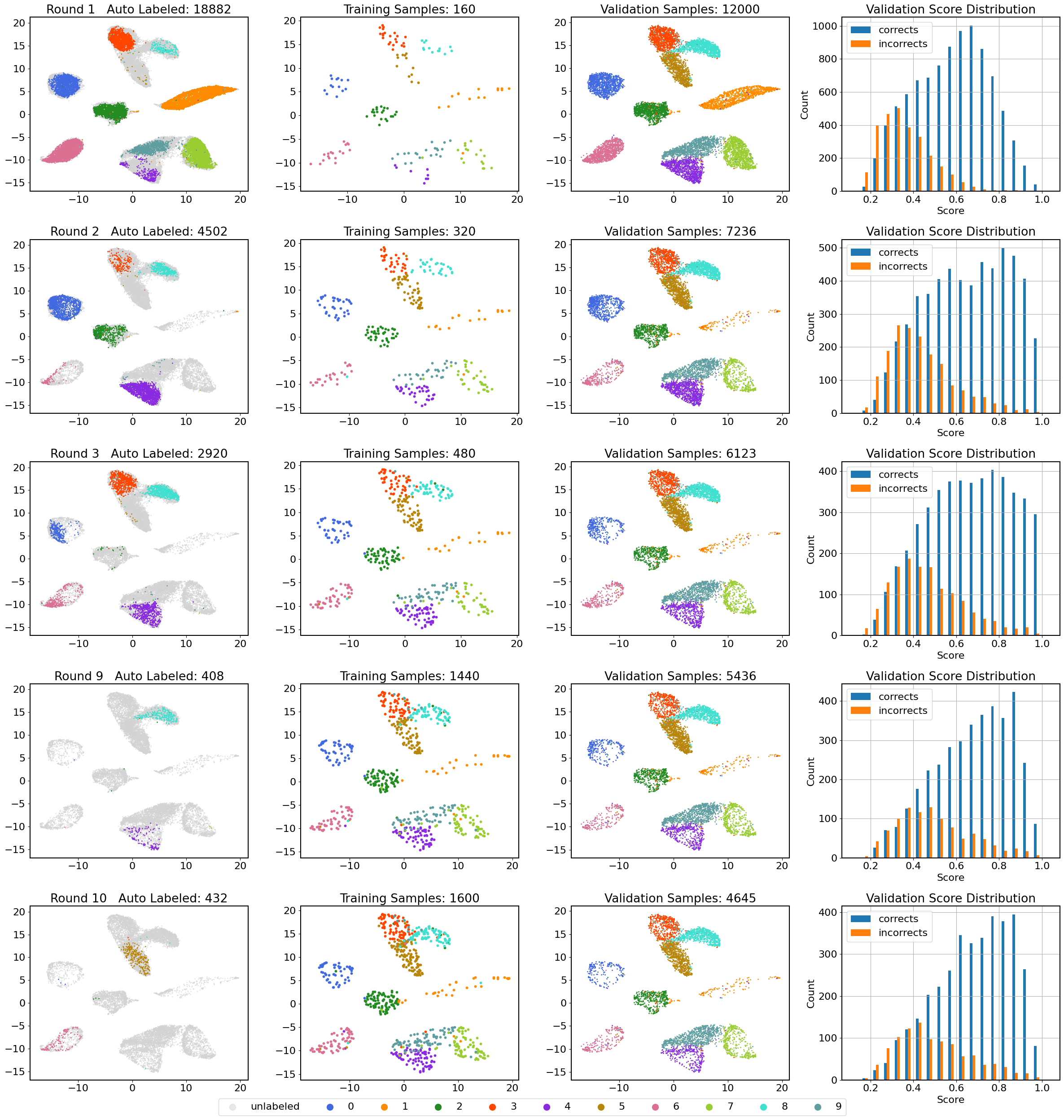
Figure 7: Auto-labeling MNIST data using linear classifier. Validation size = 12k. Maximum training samples = 1600. Each round algorithm queries 160 samples. Coverage of auto-labeling is 62.9% with 98.0% accuracy. For the rounds we show, the test error rates are 21.4%, 13.9%, 12.5%, 10.2%, and 9.8%, respectively. For four columns (left to right), we show: a) The samples that are labeled by TBAL in this round. b) The embeddings for training samples. c) The embeddings for validation data points. d) The score distribution for the validation dataset.

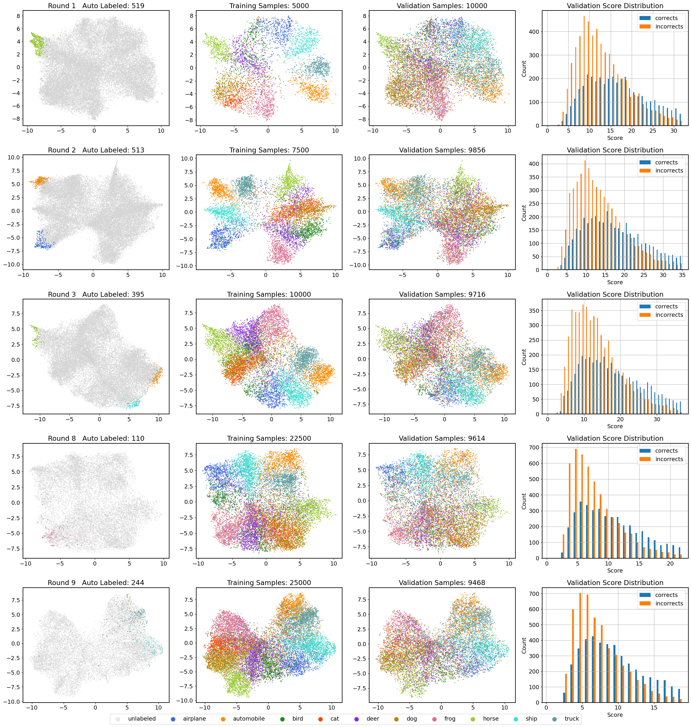
Figure 8: Auto-labeling CIFAR-10 data using a small network and energy scores. Validation size = 10k. Maximum training samples = 25k. Each round algorithm queries 2500 samples. Coverage of auto-labeling is 5.3% with 90.0% accuracy. For the rounds we show, the test error rates are 56.6%, 55.2%, 55.6%, 53.0%, and 49.3% respectively. For four columns (left to right), we show: a) The samples that are labeled by TBAL in this round. b) The embeddings for training samples. c) The embeddings for validation data points. d) The score distribution for the validation dataset.

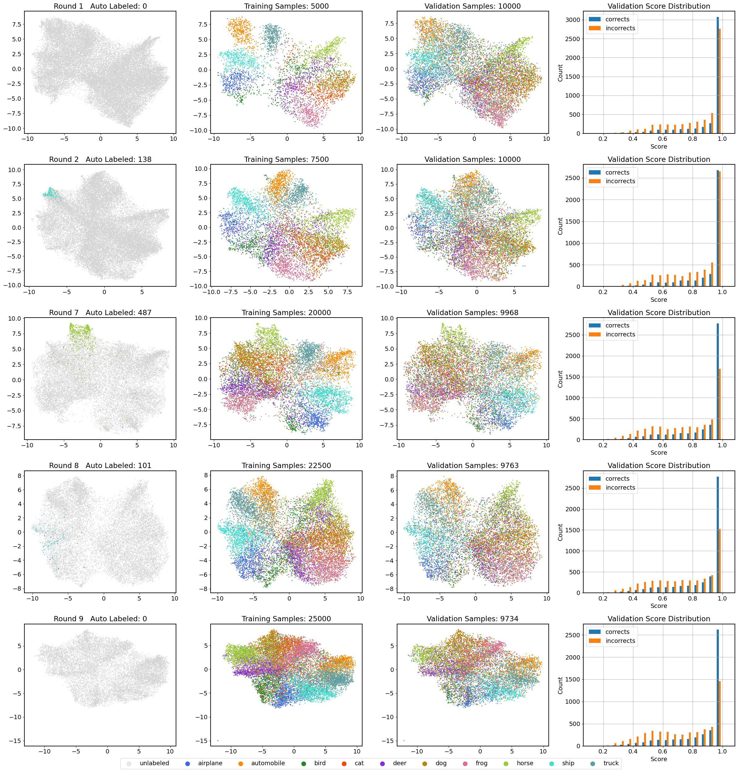
Figure 9: Auto-labeling CIFAR-10 data using a small network and softmax scores. Validation size = 10k. Maximum training samples = 25k. Each round algorithm queries 2500 samples. Coverage of auto-labeling is 2.3% with 91.0% accuracy. For the rounds visualized here in each row, the test error rates of the trained classifiers are 56.6%, 59.1%, 52.8%, 50.5%, and 51.7% respectively. For four columns (left to right), we show: a) The samples that are labeled by TBAL in this round. b) The embeddings for training samples. c) The embeddings for validation data points. d) The score distribution for the validation dataset.

References

- Air [22] Airbus. Airbus active labeling blog. https://acubed.airbus.com/blog/wayfinder/automatic-data-labeling-strategies-for-vision-based-machine-learning-and-ai/ , 2022. Accessed: 2022-11-18.
- BBZ [07] Maria-Florina Balcan, Andrei Z. Broder, and Tong Zhang. Margin based active learning. In COLT, 2007.
- BDL [09] Alina Beygelzimer, Sanjoy Dasgupta, and John Langford. Importance weighted active learning. In Proceedings of the 26th annual international conference on machine learning, pages 49–56, 2009.
- BL [13] Maria-Florina Balcan and Phil Long. Active and passive learning of linear separators under log-concave distributions. In Conference on Learning Theory, pages 288–316. PMLR, 2013.
- CAL [94] David Cohn, Les Atlas, and Richard Ladner. Improving generalization with active learning. Machine Learning, 15(2):201–221, 1994.
- CDG+ [21] Gui Citovsky, Giulia DeSalvo, Claudio Gentile, Lazaros Karydas, Anand Rajagopalan, Afshin Rostamizadeh, and Sanjiv Kumar. Batch active learning at scale. In Advances in Neural Information Processing Systems, volume 34, pages 11933–11944, 2021.
- CDM [16] Corinna Cortes, Giulia DeSalvo, and Mehryar Mohri. Learning with rejection. In International Conference on Algorithmic Learning Theory, pages 67–82. Springer, 2016.
- Cho [70] C Chow. On optimum recognition error and reject tradeoff. IEEE Transactions on information theory, 16(1):41–46, 1970.
- CKNS [15] Kamalika Chaudhuri, Sham M. Kakade, Praneeth Netrapalli, and Sujay Sanghavi. Convergence rates of active learning for maximum likelihood estimation. In Proceedings of the 28th International Conference on Neural Information Processing Systems, 2015.
- Das [06] Sanjoy Dasgupta. Coarse sample complexity bounds for active learning. In Y. Weiss, B. Schölkopf, and J. Platt, editors, Advances in Neural Information Processing Systems, volume 18. MIT Press, 2006.
- Das [11] Sanjoy Dasgupta. Two faces of active learning. Theoretical Computer Science, 412(19):1767–1781, 2011. Algorithmic Learning Theory (ALT 2009).
- DDS+ [09] Jia Deng, Wei Dong, Richard Socher, Li-Jia Li, Kai Li, and Li Fei-Fei. Imagenet: A large-scale hierarchical image database. In 2009 IEEE Conference on Computer Vision and Pattern Recognition (CVPR), pages 248–255, 2009.
- Den [12] Li Deng. The mnist database of handwritten digit images for machine learning research. IEEE Signal Processing Magazine, 29(6):141–142, 2012.
- DKM [05] Sanjoy Dasgupta, Adam Tauman Kalai, and Claire Monteleoni. Analysis of perceptron-based active learning. In International conference on computational learning theory, pages 249–263. Springer, 2005.
- DMS [15] Giulia DeSalvo, Mehryar Mohri, and Umar Syed. Learning with deep cascades. In Proceedings of the Twenty-Sixth International Conference on Algorithmic Learning Theory (ALT 2015), 2015.
- EYW [10] Ran El-Yaniv and Yair Wiener. On the foundations of noise-free selective classification. JMLR, 11:1605–1641, aug 2010.
- EYW [12] Ran El-Yaniv and Yair Wiener. Active learning via perfect selective classification. Journal of Machine Learning Research, 13(2), 2012.
- FCS+ [20] Daniel Y. Fu, Mayee F. Chen, Frederic Sala, Sarah M. Hooper, Kayvon Fatahalian, and Christopher Ré. Fast and three-rious: Speeding up weak supervision with triplet methods. In Proceedings of the 37th International Conference on Machine Learning (ICML 2020), 2020.
- Fel [43] William Feller. Generalization of a probability limit theorem of cramér. In Transactions of the American Mathematical Society, pages 361–372,, 1943.
- Fra [67] S. Fralick. Learning to recognize patterns without a teacher. IEEE Transactions on Information Theory, 13(1):57–64, 1967.
- GC [92] Olivier Gascuel and Gilles Caraux. Distribution-free performance bounds with the resubstitution error estimate. Pattern Recognition Letters, 13(11):757–764, 1992.
- GEY [17] Yonatan Geifman and Ran El-Yaniv. Selective classification for deep neural networks. In Advances in Neural Information Processing Systems, volume 30, 2017.
- GEY [19] Roei Gelbhart and Ran El-Yaniv. The relationship between agnostic selective classification, active learning and the disagreement coefficient. The Journal of Machine Learning Research, 20(1):1136–1173, 2019.
- GTA+ [21] Jakob Gawlikowski, Cedrique Rovile Njieutcheu Tassi, Mohsin Ali, Jongseok Lee, Matthias Humt, Jianxiang Feng, Anna Kruspe, Rudolph Triebel, Peter Jung, Ribana Roscher, et al. A survey of uncertainty in deep neural networks. arXiv preprint arXiv:2107.03342, 2021.
- HAB [18] Matthias Hein, Maksym Andriushchenko, and Julian Bitterwolf. Why relu networks yield high-confidence predictions far away from the training data and how to mitigate the problem. 2018.
- Han [07] Steve Hanneke. A bound on the label complexity of agnostic active learning. ICML, 2007.
- Han [14] Steve Hanneke. Theory of disagreement-based active learning. Found. Trends Mach. Learn., 7(2–3):131–309, jun 2014.
- Hsu [10] Daniel Joseph Hsu. Algorithms for active learning. PhD thesis, UC San Diego, 2010.
- Kää [06] Matti Kääriäinen. Active learning in the non-realizable case. In International Conference on Algorithmic Learning Theory, pages 63–77. Springer, 2006.
- KAH+ [17] Akshay Krishnamurthy, Alekh Agarwal, Tzu-Kuo Huang, Hal Daumé III, and John Langford. Active learning for cost-sensitive classification. In International Conference on Machine Learning, pages 1915–1924. PMLR, 2017.
- KFGR [21] Jannik Kossen, Sebastian Farquhar, Yarin Gal, and Tom Rainforth. Active testing: Sample-efficient model evaluation. International Conference on Machine Learning, 2021.
- KH+ [09] Alex Krizhevsky, Geoffrey Hinton, et al. Learning multiple layers of features from tiny images. 2009.
- KSZJJ [21] Julian Katz-Samuels, Jifan Zhang, Lalit Jain, and Kevin Jamieson. Improved algorithms for agnostic pool-based active classification. In International Conference on Machine Learning, pages 5334–5344. PMLR, 2021.
- KT [20] Ranganath Krishnan and Omesh Tickoo. Improving model calibration with accuracy versus uncertainty optimization. Advances in Neural Information Processing Systems, 33:18237–18248, 2020.
- LBBH [98] Yann LeCun, Léon Bottou, Yoshua Bengio, and Patrick Haffner. Gradient-based learning applied to document recognition. Proceedings of the IEEE, 86(11):2278–2324, 1998.
- LCH+ [06] Yann LeCun, Sumit Chopra, Raia Hadsell, M Ranzato, and Fujie Huang. A tutorial on energy-based learning. Predicting structured data, 1(0), 2006.
- LT [91] Michel Ledoux and Michel Talagrand. Probability in banach spaces. 1991.
- MDR+ [21] Matthias Minderer, Josip Djolonga, Rob Romijnders, Frances Hubis, Xiaohua Zhai, Neil Houlsby, Dustin Tran, and Mario Lucic. Revisiting the calibration of modern neural networks. In Advances in Neural Information Processing Systems, volume 34, pages 15682–15694, 2021.
- MHX+ [21] Chunwei Ma, Ziyun Huang, Jiayi Xian, Mingchen Gao, and Jinhui Xu. Improving uncertainty calibration of deep neural networks via truth discovery and geometric optimization. In Proceedings of the Thirty-Seventh Conference on Uncertainty in Artificial Intelligence, volume 161 of Proceedings of Machine Learning Research, pages 75–85. PMLR, 27–30 Jul 2021.
- ML [18] Stephen Mussmann and Percy Liang. On the relationship between data efficiency and error for uncertainty sampling. In Proceedings of the 35th International Conference on Machine Learning, ICML, 2018.
- MRT [12] Mehryar Mohri, Afshin Rostamizadeh, and Ameet Talwalkar. Foundations of Machine Learning. The MIT Press, 2012.
- Pla [99] John Platt. Probabilistic outputs for support vector machines and comparisons to regularized likelihood methods. Advances in large margin classifiers, 10(3):61–74, 1999.
- PyT [22] PyTorch. Cifar-10 pytorch tutorial. https://pytorch.org/tutorials/beginner/blitz/cifar10_tutorial.html, 2022. Accessed: 2022-11-18.
- PZ [21] Nikita Puchkin and Nikita Zhivotovskiy. Exponential savings in agnostic active learning through abstention. Proceedings of Machine Learning Research, pages 3806–3832. PMLR, 2021.
- QCG [20] Hang Qiu, Krishna Chintalapudi, and Ramesh Govindan. Minimum cost active labeling. arXiv preprint arXiv:2006.13999, 2020.
- RBE+ [18] Alexander Ratner, Stephen H. Bach, Henry Ehrenberg, Jason Fries, Sen Wu, and Christopher Ré. Snorkel: Rapid training data creation with weak supervision. In Proceedings of the 44th International Conference on Very Large Data Bases (VLDB), Rio de Janeiro, Brazil, 2018.
- RF [17] Joseph Redmon and Ali Farhadi. YOLO9000: better, faster, stronger. In 2017 IEEE Conference on Computer Vision and Pattern Recognition (CVPR), pages 6517–6525, 2017.
- RSW+ [16] A. J. Ratner, Christopher M. De Sa, Sen Wu, Daniel Selsam, and C. Ré. Data programming: Creating large training sets, quickly. In Proceedings of the 29th Conference on Neural Information Processing Systems (NIPS 2016), Barcelona, Spain, 2016.
- RXC+ [20] Pengzhen Ren, Yun Xiao, Xiaojun Chang, Po-Yao Huang, Zhihui Li, Brij B. Gupta, Xiaojiang Chen, and Xin Wang. A survey of deep active learning, 2020.
- SA [22] Superb-AI. Superb ai automated data labeling service. https://www.superb-ai.com/product/automate, 2022. Accessed: 2022-11-18.
- Set [09] Burr Settles. Active learning literature survey. 2009.
- SGJ [21] Shubhanshu Shekhar, Mohammad Ghavamzadeh, and Tara Javidi. Active learning for classification with abstention. IEEE Journal on Selected Areas in Information Theory, 2(2):705–719, 2021.
- SGT [22] SGT. Aws sagemaker ground truth. https://aws.amazon.com/sagemaker/data-labeling/, 2022. Accessed: 2022-11-18.
- SK [19] Nabeel Seedat and Christopher Kanan. Towards calibrated and scalable uncertainty representations for neural networks. arXiv preprint arXiv:1911.00104, 2019.
- SM [20] Kulin Shah and Naresh Manwani. Online active learning of reject option classifiers. Proceedings of the AAAI Conference on Artificial Intelligence, 34(04):5652–5659, 2020.
-
SS [22]
Samsung-SDS.
Samsung sds auto-labeling service.
https://www.samsungsds.com/en/insights/
TechToolkit_2021_Auto_Labeling.html , 2022. Accessed: 2022-11-18. - TK [01] Simon Tong and Daphne Koller. Support vector machine active learning with applications to text classification. Journal of machine learning research, 2(Nov):45–66, 2001.
- VLK+ [21] Rudy Venguswamy, Mike Levy, Anirudh Koul, Satyarth Praveen, Tarun Narayanan, Ajay Krishnan, Jenessa Peterson, Siddha Ganju, and Meher Kasam. Curator: A No-Code Self-Supervised Learning and Active Labeling Tool to Create Labeled Image Datasets from Petabyte-Scale Imagery. In EGU General Assembly Conference Abstracts, pages EGU21–6853, April 2021.
- VSP+ [17] Ashish Vaswani, Noam Shazeer, Niki Parmar, Jakob Uszkoreit, Llion Jones, Aidan N. Gomez, Lukasz Kaiser, and Illia Polosukhin. Attention is all you need. In Proceedings of the 30th Conference on Neural Information Processing Systems (NIPS 2017), 2017.
- WEY [11] Yair Wiener and Ran El-Yaniv. Agnostic selective classification. Advances in neural information processing systems, 24, 2011.
- WEY [15] Yair Wiener and Ran El-Yaniv. Agnostic pointwise-competitive selective classification. Journal of Artificial Intelligence Research, 52:171–201, 2015.
- WFZ [21] Deng-Bao Wang, Lei Feng, and Min-Ling Zhang. Rethinking calibration of deep neural networks: Do not be afraid of overconfidence. In Advances in Neural Information Processing Systems, volume 34, pages 11809–11820, 2021.
- WHRS [21] Yingfan Wang, Haiyang Huang, Cynthia Rudin, and Yaron Shaposhnik. Understanding how dimension reduction tools work: An empirical approach to deciphering t-sne, umap, trimap, and pacmap for data visualization. Journal of Machine Learning Research, 22(201):1–73, 2021.
- WLW [03] Ting-Fan Wu, Chih-Jen Lin, and Ruby Weng. Probability estimates for multi-class classification by pairwise coupling. Advances in Neural Information Processing Systems, 16, 2003.
- ZN [22] Yinglun Zhu and Robert Nowak. Efficient active learning with abstention. arXiv preprint arXiv:2204.00043, 2022.
- ZT [21] Yufan Zeng and Jiashan Tang. Rlc-gnn: An improved deep architecture for spatial-based graph neural network with application to fraud detection. Applied Sciences, 11, 06 2021.