Spatial-temporal dynamics of employment shocks in declining coal mining regions and potentialities of the ‘just transition’

Abstract

The United States, much like other countries around the world, faces significant obstacles to achieving a rapid decarbonization of its economy. Crucially, decarbonization disproportionately affects the communities that have been historically, politically, and socially embedded in the nation’s fossil fuel production. However, this effect has rarely been quantified in the literature. Using econometric estimation methods that control for unobserved heterogeneity via two-way fixed effects, spatial effects, heterogeneous time trends, and grouped fixed effects, we demonstrate that mine closures induce a significant and consistent contemporaneous rise in the unemployment rate across US counties. A single mine closure can raise a county’s unemployment rate by 0.056 percentage points in a given year; this effect is amplified by a factor of four when spatial econometric dynamics are considered. Although this response in the unemployment rate fades within 2-3 years, it has far-reaching effects in its immediate vicinity. Furthermore, we use cluster analysis to build a novel typology of coal counties based on qualities that are thought to facilitate a successful recovery in the face of local industrial decline. The combined findings of the econometric analysis and typology point to the importance of investing in alternative sectors in places with promising levels of economic diversity, retraining job seekers in places with lower levels of educational attainment, providing relocation (or telecommuting) support in rural areas, and subsidizing childcare and after school education programs in places with low female labor force participation due to the gendered division of domestic work.

1 Introduction

The burning of fossil fuels in the United States (US) accounted for 13.5% of global CO2 energy combustion emissions in 2020, led domestically by oil (43%), gas (35%), and coal (19%), with flaring, cement production and other industrial processes accounting for the final 3% [21]. Having generated approximately a quarter of all global cumulative carbon dioxide (CO₂) emissions since 1750, the country’s outsized historical responsibility to decarbonize its economy over the next three decades – consistent with national commitments under the 2015 Paris Agreement – is largely incontrovertible.

In 2021, President Joe Biden committed his administration to decarbonizing the US economy by decreasing greenhouse gas emissions to 50-52% below 2005 levels by 2030 with a view towards net-zero emissions by 2050 [57]. In August 2022, the Inflation Reduction Act (IRA) was passed constituting a significant step in the direction of these ambitious goals, aiming jointly to reduce inflation, lower prescription medicine prices, and invest heavily in domestic energy production with a focus on clean energy. Climate and energy security investments stipulated in the IRA total 369 billion US$ [19].

As the political momentum behind decarbonization increases, the question of how to usher in a ‘Just Transition’ – ensuring minimal damage from and the equitable sharing of the benefits of decarbonization — is front of mind for environmental and climate justice advocates concerned about impacts on workers, consumers, and frontline communities [44, 37, 49, 52, 16]. The IRA makes several long-awaited commitments for consumers and frontline communities, including reducing legacy pollution through block grants, reinstating Superfund taxes to fund toxic site clean-ups and air pollution monitoring, and making clean energy more affordable and accessible for disadvantaged communities. Notwithstanding, environmental justice advocates worry that many of the compromises required to ensure that the IRA was passed, including a guarantee to continue federal oil and gas leasing, could significantly outweigh these benefits [46, 18].

The IRA’s Just Transition provisions for vulnerable workers are more difficult to discern. The International Energy Agency predicts 50,000 layoffs in the US coal sector by 2030 while up to a quarter million US oil and gas jobs are also threatened [2]. Because fossil fuel deposits are highly concentrated geographically, a decline in output will be felt most sharply in a few select regions with deep roots in the fossil fuel industry [26, 62, 55]. Although the IRA lists several generic initiatives to support American workers, including tax incentives for domestic manufacturing and credits for businesses that pay prevailing wages, only two policy objectives can be described as targeting fossil fuel workers specifically: a 10% increase in the clean energy tax credit for infrastructure projects operating in or near ”energy communities” and a 5 billion US$ fund providing low-cost loans and refinancing for energy infrastructure, with the notable caveat that qualifying projects should “retool, repower, repurpose, or replace energy infrastructure that has ceased operations” [19].

These measures are a just small sample of a larger set of proposed Just Transition policy responses that range from completely compensatory (i.e. direct income support, relocation assistance, interim health care coverage, pension payouts) to active labor market policies (i.e. education, training, and reskilling) and investments in alternative sectors, whether green or otherwise, to provide new job opportunities [51, 49, 52, 53].

To optimize Just Transition aid for at-risk workers, policymakers need to compare available ameliorative measures based on the magnitude, durability, and spatial distribution of adverse employment impacts. While numerous qualitative studies have proffered various conceptualizations of energy justice and ethical principles to guide a ‘Just Transition’ amid structural decarbonization [25, 30], econometric evidence exploring these real-world barriers to transitional justice is scarce. In-depth regional investigation of the effects of fossil energy industry reliance on employment has generally been done qualitatively, through vulnerability assessments or sociological and ethnographic analyses [9, 1, 13, 14, 61, 62, 54, 63]. The available econometric research has mostly concentrated on oil and gas, specifically oil prices and the macroeconomy [24]. For example, the tight oil and shale gas booms in the early 2000s have garnered the attention of most quantitative studies on employment impacts of fluctuations in fossil fuel production [36, 68, 42, 45, 38]. Furthermore, such results are rarely framed from the Just Transition perspective until a recent study by Scheer et al linked econometric evidence explicitly to the literature through an examination of employment precarity in oil-rich Alberta [59].

We therefore aim to fill this critical evidentiary gap through an in-depth examination of the already experienced, prolonged, and consistent contraction in US coal production. We make three significant contributions to existing literature. We first contribute empirical econometric evidence to elucidate the relevant Just Transition issues, exploring the spatio-temporal nature of coal transitions and employment dynamics in order to illuminate the relative usefulness of proposed policy interventions, including those in the IRA. Second, to the best of our knowledge, ours is also the first panel econometric study to assess the employment impacts of coal mine closures in the US. Most similar to our work, is the examination by Black et al [11] comparing coal and non-coal producing counties in four states during the boom, peak, and fall of the coal industry in the 1970s and 1980s. Other panel studies on US coal production focus mainly on market dynamics and coal productivity or health and safety [64, 31, 23]. Third, we establish a typology of coal mining communities to inform future research and policymaking in a period of accelerating energy transitions. To our knowledge, two other studies have defined comparable typologies using theoretical frameworks. Snyder employs three indicators to proxy education, poverty, and rurality, while Raimi proposes twelve [62, 54]. Our work supplements existing literature by presenting an intermediate number of vulnerability axes, striking a balance between multidimensionality and succinctness; by operationalizing the typology through hierarchical clustering analysis; and by reincorporating our typology into our econometric analysis.

Evaluating the magnitude, persistence, and geographic distribution of employment shocks following mine closures requires a tailor-fit econometric modelling approach that minimizes confounding from unobserved spatial and temporal dependencies. Therefore, we use dynamic panel econometric and spatial econometric methods to assess employment impacts. These methods enable us to account for latent common factors and spatial spill-over effects and achieve greater precision in the estimation of employment shocks caused by structural changes to the US coal sector. We also use machine learning techniques of agglomerative hierarchical clustering to analyse the prominent characteristics of coal mining communities to improve Just Transition policymaking. By integrating clustering analysis with econometrics, we may examine how coal mine closures affect different ’categories’ of counties in different ways. Complementarily, we explore the merit of the assumption that green economy investments are sufficient to ensure the stability and prosperity of transitioning fossil fuel producing communities by analysing whether proximate renewable energy investments mitigate unemployment growth following mine closures. The significance of this final question is made all the more relevant given that this assumption underlies one of the main policy provisions of the IRA targeting energy communities.

In what follows, we first describe the data sources and variables used in the econometric and cluster-typological analyses. After discussing our empirical strategy for estimating several panel data models using a suite of purpose-fit specifications, we describe our motivation and method for creating a typology of US coal counties. The study concludes by discussing policy implications and context-dependent policy recommendations based on our combined econometric and cluster-typological analyses.

2 Data

2.1 Econometric Estimation

First, a panel dataset was created using economic variables from the US Department of Commerce’s Bureau of Economic Analysis (BEA), the US Bureau of Labor Statistics (BLS), and the US Census Bureau for 3,072 contiguous US counties from 2002 to 2019. Annual data on active mines in each county came from the Energy Information Administration (EIA) and the Mine Safety and Health Administration (MSHA). The change in the number of active mines in a county in a given year is the main independent variable of interest. The BLS reports the county unemployment rate change from the prior year, our main dependent variable (Table 1: Model 1). As dependent variables, we additionally investigate the change in the natural log of employed persons, unemployed persons, total labor force, and population size (Table 1: Models 2 to 5). Appropriate combinations of real GDP per capita, real GDP, and population (all in natural log) were included as control variables in each model.

Furthermore, the US Department of Agriculture maintains an energy investment database containing “information regarding USDA programs that provide assistance to renewable energy and efficiency projects” at state, county, and congressional district levels. Since 2002, the USDA has reported a total investment in renewable energy projects of 6.3 trillion US$ in the contiguous US, or 20.7 US$ per capita. Only 122.2 million US$ (7.5 US$ per capita), or 2%, of these investments were allocated to coal counties while non-coal counties benefitting from investments received 25.1 US$ per capita. For the purpose of this study, investments in renewable energy were retained and energy efficiency improvements were removed as they largely represented improvements in on-farm agricultural practices which were deemed unlikely to impact coal workers. The variable of interest derived from this data source is a binary indicator for whether county-level renewable energy investments exceed 0.1% of county real GDP in a particular year.

Additionally, the US Census Bureau maintains a county adjacency file for all US counties indicating which counties share a border. This adjacency file was adapted to incorporate information on contiguous US counties when estimating Models 1-5^{[SEM, SLM, SARAR]} as outlined in Table 1.

2.2 Typology

A dataset of selected social, economic, and political characteristics of the contiguous counties observed in the panel dataset was sourced from the US Census Bureau, US Department of Agriculture, the MIT Election Data and Science Lab, and Chmura, a private producer of economic data that imputes a county-level economic diversity index. Selected variables include educational attainment, population size, median incomes, female labor force participation, economic diversity, rural-urban classification, and political party affiliation.

Appendices A.1 and A.2 of the Supplementary Materials provide details on the indicators, surveys, and data sources used.

3 Methods

This study’s panel data analysis is based on six baseline model specifications. Table 1 provides algebraic formulas and technical details of each. All models were estimated using the previously described county-level panel dataset covering 2002 to 2019. Several models (denoted by * in Table 1) were estimated on a subset of coal counties, defined as counties that had active mines between 2002 and 2019. The model specifications are motivated as follows:

• Model 1 evaluates if a change in the number of active mines affects county unemployment rate.

• Models 2-5 aim to identify through what channel the unemployment rate varies due to a change in active mines (i.e., a change in the number of employed workers or in the size of the labour force). This is studied by regressing the county unemployment rate determinants (number of employed persons, number of unemployed persons, labour force size, and population size) on the same indicators for changes in active mines.

• Model 6 evaluates whether county-level renewable energy investments have lessened the magnitude of employment losses following coal mine closures.

Models 1-6 (without superscripts) were estimated using the classic two-way fixed effects (TWFE) estimator, with standard errors clustered by county and year to address within-cluster correlation and heteroskedasticity. Prior to model estimation, all variables were first-difference transformed to address non-stationarity [60, 15]. This yielded stationary I(0) covariates, with the additional benefit that the effects of first-difference variables are easy to interpret.

Within this first stream of analysis, two non-negligible issues challenge the interpretation of the results of the Models 1-6: cross-sectional dependence and likely treatment effect heterogeneity.

Table 1: Model Specifications

#	Model Specification		Results
1*	$\Delta UER_{it}=\boldsymbol{\beta}\begin{pmatrix}\boldsymbol{X}_{it}\\ \Delta log(RealGDPPC)_{it}\\ \end{pmatrix}+\alpha_{i}+\gamma_{t}+\varepsilon_{it}$		Figure 1-2 Appendix B.1.2: Tables 13-14
2*	$\Delta log(EmployedPersons)_{it}=$	$\boldsymbol{\beta}\begin{pmatrix}\boldsymbol{X}_{it}\\ \Delta log(RealGDP)_{it}\\ \Delta log(Population)_{it}\\ \end{pmatrix}+\alpha_{i}+\gamma_{t}+\varepsilon_{it}$	Figure 3 Appendix B.1.2: Tables 13-14
3*	$\Delta log(UnemployedPersons)_{it}=$
4*	$\Delta log(LaborForce)_{it}=$
5*	$\Delta log(Population)_{it}=\boldsymbol{\beta}\begin{pmatrix}\boldsymbol{X}_{it}\\ \Delta log(RealGDP)_{it}\\ \end{pmatrix}+\alpha_{i}+\gamma_{t}+\varepsilon_{it}$
6*	$\Delta UER_{it}=\boldsymbol{\beta}\boldsymbol{X}_{it}+\boldsymbol{Z}\begin{pmatrix}\Delta ActiveMines_{it}*REInvestments_{it}\\ \Delta ActiveMines_{it-1}*REInvestments_{it-1}\\ \Delta ActiveMines_{it-2}*REInvestments_{it-2}\\ \end{pmatrix}+\alpha_{i}+\gamma_{t}+\varepsilon_{it}$		Appendix B.1.2: Table 19
1SEM	$Y_{it}=\boldsymbol{\beta}\boldsymbol{X}_{it}+\alpha_{i}+\gamma_{t}+U_{it}$ $U_{it}=\delta W_{i}U_{t}+\varepsilon_{it}$		Figure 2 Appendix B.2: Tables 21-23, 25
1SLM	$Y_{it}=\boldsymbol{\beta}\boldsymbol{X}_{it}+\rho W_{i}Y_{t}+\alpha_{i}+\gamma_{t}+\varepsilon_{it}$
1-5SARAR	$Y_{it}=\boldsymbol{\beta}\boldsymbol{X}_{it}+\rho W_{i}Y_{t}+\alpha_{i}+\gamma_{t}+U_{it}$ $U_{it}=\delta W_{i}U_{t}+\varepsilon_{it}$
1-6HTT(d)	$Y_{it}=\boldsymbol{\beta}\boldsymbol{X}_{it}+\sum_{l=1}^{d}\lambda_{il}f(t)+\alpha_{i}+\gamma_{t}+\varepsilon_{it}$		Figure 2 Appendix B.3: Tables 26-28
Variable definitions: i : denotes each county for i=1, 2,…3,072 counties t : denotes each year for t=2002, 2003,…2019 $\boldsymbol{\alpha}_{i}$ : unit-fixed effects $\boldsymbol{\gamma}_{t}$ : time-fixed effects $\boldsymbol{X}_{it}$ : Vector of independent variables ($\Delta$ Active Minesit, $\Delta$ Active Minesit-1, $\Delta$ Active Minesit-2). For Model 6, this includes levels of all interacted variables. For Models 1-5[SEM, SLM, SARAR] and 1-6HTT(1),HTT(2)] this represents all independent variables denoted in Models 1-6, respectively. $\boldsymbol{Y}_{it}$ : Relevant dependent variable denoted by Model number. $\boldsymbol{\beta}$ : Vector of regression coefficients to be estimated. $\boldsymbol{\rho}$ : Spatial autoregression parameter. $\boldsymbol{\delta}$ : Spatial autocorrelation parameter. $\boldsymbol{W}_{i}$ : N X N spatial weight matrix for neighbors of unit i where N = 3,072. $\boldsymbol{\lambda}_{il}$ : Individual loadings parameter per unit i and factor l in heterogeneous trend models. f(t) : Unobserved time-varying common factors used in heterogeneous trend models. REInvestmentsit: dummy indicator of whether renewable energy investments exceeded 0.1% of GDPit. $\boldsymbol{\Delta}UER_{it}$ : Change in unemployment rate in county i in year t. Note: * indicates model was also applied to a subset of coal counties only.

3.1 Accommodating Cross-Sectional Dependence

The TWFE estimator, like other estimators used in ordinary least squares regression modelling, requires the restrictive condition of cross-sectional independence. In practice, any unobserved cross-section dependencies, such as structural breaks, global stochastic trends, or spatial (spill-over) effects, in the underlying data generating process are assumed to be captured sufficiently using linear additive two-way (unit and time) fixed effects. In many real-world circumstances, this assumption is too restrictive [29, 17]. Although it can accommodate time-invariant confounders, the TWFE estimator comes at the expense of potential dynamic misspecification [50]. Insufficient accounting for cross-sectional dependence can lead to inaccurate and inconsistent regression coefficient estimates [5, 48]. And indeed, this concern appears justified in the present study as several diagnostic tests could not reject the presence of significant cross-sectional dependence in Models 1-6 [3, 4, 39].

Therefore, two estimation approaches frequently used to account for cross-sectional dependence were applied to complement the TWFE OLS model results. Specifically, we use estimators that account for spatially correlated effects (SEM, SLM, and SARAR in Table 1) and one- and two-factor heterogeneous trends models (HTT(1) and HTT(2) in Table 1). Each method is described below.

3.1.1 Spatial Econometric Models

First, three spatial econometric models were estimated: a spatial autoregressive model (SLM), a spatial error model (SEM), and a spatial autoregressive model with autoregressive error structure (SARAR) [35, 8]. The latter combines the SLM and SEM models’ core features. Given the extent of spatial dependency in our data [27, 40], the SLM and SARAR models were selected as the most acceptable spatial feature specifications based on AIC and BIC information criteria. Beyond serving as a robustness check on our initial TWFE estimates, the SLM and SARAR models provide additional valuable information: namely, they tell us whether the impact of mine closures exhibit regional spill-over effects.

3.1.2 Heterogeneous Trends Models

The second method employed to accommodate cross-sectional dependence is via latent factor modelling, which assumes the panel data model exhibits a factor-analytic error structure. In this approach, one or more latent (unobserved) common factors can be estimated via iterative principal component analysis (the ”interactive fixed effects” estimator proposed in Bai (2009)), or instead, approximated via cross-sectional averages of the dependent and independent variables (the ”common correlated effects” estimator proposed in Pesaran (2006)) [47, 7, 33]. Another method is to estimate the unobserved factors semi-parametrically via functions that capture unit-specific time trends (the ”heterogeneous time trends” estimator proposed in Kneip et al (2012)). We apply the heterogeneous time trends estimator because it permits unobserved components to be non-stationary and exhibit smooth time trends. It is therefore well-suited for capturing unobserved trends related to long run energy prices, automation, and technical efficiency advances. The AIC or BIC criteria for one- and two-factor models showed no significant benefit of including more than one factor when computing heterogeneous time trends.

3.2 Accommodating Treatment Effect Heterogeneity

The TWFE estimator may also generate bias when treatment effects are entirely or partially heterogeneous across units. To properly infer the effect of a treatment variable (e.g., a change in the number of active coal mines) on a target variable (the county unemployment rate), the TWFE estimator forces the econometrician to assume the treatment effect is constant across units and time, known as the ”common trends” assumption. In the present study, there are compelling reasons to suspect that employment impacts of mine closures can vary substantially across counties for reasons other than those which we are able to capture via the aforementioned control variables. Specifically, unmodeled demographics can cause selection bias. These demographic traits need not be directly related to changes in the unemployment rate but may predict counties’ transitional capacities when mines close. By identifying weighted sums of average treatment effects in each group and period without considering the underlying reason for the variation, the TWFE estimator may not capture relevant treatment effect heterogeneities across units, leading to biased and potentially misleading coefficient estimates [17].

3.2.1 Agglomerative Hierarchical Clustering

Therefore, to address the issue of possible treatment effect heterogeneity in our sample, agglomerative hierarchical clustering analysis was performed on the typology dataset containing information on salient demographic characteristics of the 252 counties identified as coal counties as well as the total set of 3,072 contiguous US counties [32, 43, 56]. Prior to running the clustering analysis, the indicators used were scaled or standardized to have a mean of zero and standard deviation of one. Applying three of the most common methods (elbow, silhouette, and gap statistic) for determining the optimal number of clusters to identify yielded inconclusive results for the coal counties, proposing between two and four clusters [58, 65]. In the case of the complete contiguous US dataset the three tests to identify the optimal number of clusters revealed consistent results, suggesting three as the optimal number of clusters. Thus, to aid in an eventual comparison of coal counties to US counties overall, each dataset was clustered into three “types.” Variables considered in the clustering analysis include an urban/rural index, population size, educational attainment, economic security, female labor force participation, economic diversity, and political attitudes.

This hierarchical clustering serves a dual purpose. First, the resulting ‘cluster membership’ information obtained from the tripartite typology of coal counties was used to re-estimate Model 1 using grouped fixed effects, allowing for partially heterogeneous slope coefficients for each independent variable of interest. Second, we present a constructed typology that sheds light on the diversity and geographical distribution of various challenges faced by coal communities across the US.

The results of all aforementioned regressions (Appendices B and D), tests (Appendix C), model selection methods (Appendix B.2), and clustering (Appendices C.3 and D) can be found in the Supplementary Materials.

4 Results

4.1 Two-Way Fixed Effects, Spatial, and Heterogeneous Trends Econometric Models

When estimating the models presented in Table 1, we expect that the closure of a coal mine would spark an increase in the county-level unemployment rate. Such an effect is unlikely to occur solely because of employment losses in the coal industry specifically but likely in combination with spill-over effects from such employment losses onto the jobs and livelihoods of those whose work is conducted in support of coal county functioning (i.e., education, services, retail). This hypothesis is consistent with macroeconomic theory positing that there are direct, indirect, and induced jobs associated with a given economic activity [6].

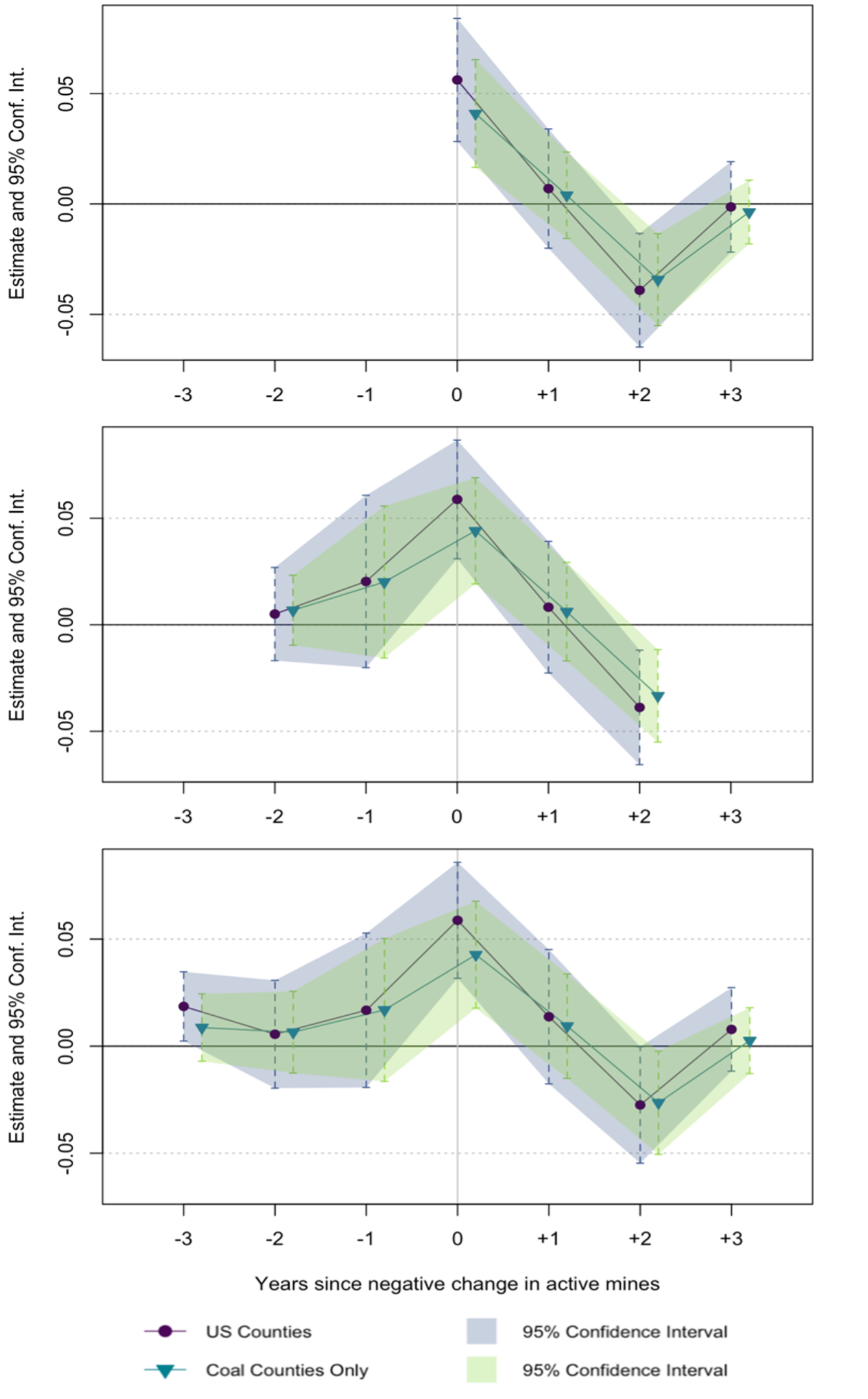
Figure 1: Figure 1 illustrates the sequence of responses in county unemployment rate to a change in active mines at time t = 0 and associated 95% confidence intervals. For simplified interpretation, the sign of the impact has been flipped to illustrate the change in unemployment rate resulting from a decrease in active mines. The y-axis indicates the time since the change in active mines was reported. Three combinations of lags and leads have been included for illustrative purposes as they do not significantly change the principal coefficient estimates at times t, t-1, and t-2. Exact coefficients are reported in Tables 12 and 13 of Appendix B.1.2 of the Supplementary Materials.

Model 1 finds that a single mine closure (one-unit decrease in the number of active mines) is associated with a 0.056 (0.041; restricted coal county sample in parentheses) percentage point increase in county unemployment rate. For the model using all US counties (coal counties only), we reject the null hypothesis of no effect at the 0.1% (1%) level. When evaluating dynamics, the unemployment rate neither seems to continue to increase nor recover a year after mine closures are reported with a further change in unemployment rate imperceptibly different from zero. However, two years later, the unemployment rate appears to recover slightly, decreasing by 0.039 (0.034) percentage points at a 1% (1%) level of statistical significance on the dataset of all US counties (coal counties). A linear combination of the coefficient estimates confirms the non-persistent nature of the unemployment rate change. Coefficient estimates are reported in Figure 1 of the main text and Tables 13 and 14 of Appendix B.1.2 of the Supplementary Materials.

Figure 2 compares coefficient estimates reported by Models 1, 1^{[SEM, SLM, SARAR]}, and 1^{[HTT(1), HTT(2)]} models along with their respective 95% confidence intervals. The coefficients reported in Figure 2 for Model 1^SLM and Model 1^SARAR are the direct (intra-county) and indirect (inter-county) impacts of a change in active mines in a particular county, reported separately. The direction of responses in the unemployment rate are consistent across all estimations, providing substantial validation of the sign of the coefficient estimates derived from Models 1-6. Although the SLM and SARAR models estimate the direct impact of mine closures to be slightly smaller in magnitude (significant at the 0.1% level for a closure in time t and t-2), the indirect and combined total impacts are consistently larger, indicating the presence of strong spatial diffusion of impacts not identifiable in the TWFE model. Model 1^SARAR, for example, finds a contemporaneous 0.215 percentage point increase in unemployment rate from a one-unit decrease in active mines in a neighbouring county, 6 times greater than the direct impact identified by the same model. This spatial diffusion echoes results in previous applications of spatial econometric models to US employment data [12].

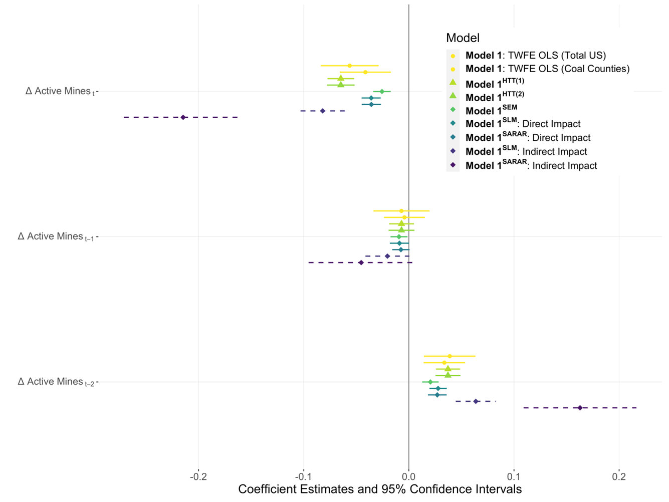
Figure 2: Coefficient estimates and corresponding 95% confidence intervals represent the response of unemployment rate to a change in active mines in times t, t-1, and t-2 as estimated by each model estimation. Confidence intervals for “indirect” impacts calculated from the SLM and SARAR models are represented by dashed lines.

Similarly, the coefficient estimates of the heterogeneous trends models are greater in the same year in which a change in active mines occurs. More precisely, the one-factor heterogeneous trends model Model 1^HTT(1) reports that a one-unit decrease in the number of active mines is associated with a 0.064 percentage point increase in unemployment rate at a 0.1% level of statistical significance. Given that heterogeneous trends models have a de-biasing effect on coefficient estimates due to the consideration of unobserved latent factors, this result indicates that the response in unemployment rate in the same year as a change in active mines is likely underestimated in Model 1. In short, the spatial and heterogeneous trends models indicate a significant underestimation of the true contemporaneous impact of a mine closure on county unemployment rate. The heterogeneous trends models indicate that the estimate is nearly 1.2 times greater and the spatial models indicate that much of this unemployment rate spike is reflected in neighbouring counties. Coefficient estimates of Models 1^{[SEM, SLM, SARAR]} and Models 1^{[HTT(1), HTT(2)]} are represented in Figure 2 and can be found in Appendices B.2 and B.3, respectively, of the Supplementary Materials.

To add further detail, asymmetric estimation was carried out to evaluate whether increases and decreases of active mines have symmetric effects. The regression results of each of these estimations is provided in Tables 17 and 18 of Appendix B.1.2 in the Supplementary Materials and show that the magnitude and statistical significance of a response in the unemployment rate to a change in active mines is mainly attributable to a negative change. Linearly combining the coefficient estimates confirms this finding and reveals further illuminating results. First, when incorporating a factor for whether the change was negative, the magnitude of change in time t = 0 increases in magnitude to 0.075 percentage points (compared to 0.056 percentage points in Model 1) at the 1% significance level. Second, when incorporating a factor for whether the change in mines was positive, the magnitude of change decreases in magnitude to just –0.019% and is no longer statistically significant. Altogether, this asymmetric treatment model indicates minimal, if any, employment benefits from counteracting a coal phase-out.

4.2 Putting It Into Context: Determinants of the Unemployment Rate Response

Our initial results do not reveal which determinants of unemployment rate might be causing these responses to mine closures. To answer this question, we considered the main variables used to calculate the rate: unemployed persons, employed persons, and total labor force (the sum of employed and unemployed persons). Their relationship is defined by Equation 1 below:

$$Unemployment\>Rate=\frac{Unemployed\>Persons}{Unemployed+Employed\>Persons}=\frac{Unemployed\>Persons}{Labor\>Force}$$ (1)

The sign and statistical significance of the change in each variable 0, 1, and 2 years following a mine closure are reported in Figure 3.

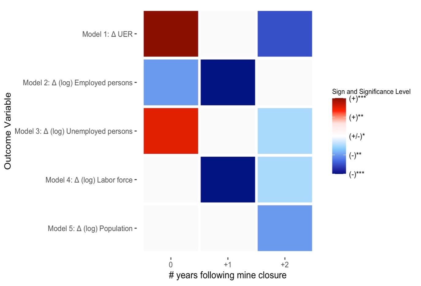
Figure 3: This figure indicates the direction of changes (red = increase; blue = decrease) in the unemployment rate, natural log of employed persons, natural log of unemployed persons, natural log of labor force, and natural log of population at the county level from a change in active mines at time t, t-1, and t-2. The sign of the response variable has been flipped to allow for interpretation of the sign as the response to a decrease in the number of active mines. The sign and magnitude of the response is reported from the model run on all US counties. Significance codes are reported as follows: *** 0.1%, **1%; *5%. A grey box indicates an insignificant variable response.

First, in the year when the change in active mines is reported, the change in unemployment rate is found to most likely be caused by a reshuffling of the labor force from employed to unemployed persons, or lay-offs, rather than any change in the size of the labor force or population overall.

In the following year, the unemployment rate neither continues to increase nor recover. The only two detectable changes in the factors of the unemployment rate are further decreases in employed persons and labor force size. This not only indicates that employment continues to decrease but also that those leaving employment are not entering unemployment and therefore likely either become discouraged, retire, or move to another county. However, there is no discernible change in population size, and it is therefore more likely that the shrinking labor force indicates either discouraged or retired workers leaving the category of employed persons. Although the magnitude of change in population size discerned in our study is small, such a theory is consistent with well-documented underemployment challenges in coal regions like Appalachia [69].

Finally, two years following a change in active mines, we observe a small decrease (or partial recovery) in county unemployment rate in Model 1. However, Figure 3 suggests that this is not principally determined by a re-entry of unemployed persons into employment. Rather, a further shrinking of the labor force and decrease in unemployed persons considered together with a small decrease in overall population size indicates that workers might be moving to meet other job opportunities. This result echoes findings that local demand shocks induce a stock equilibrium shift through migration such that the relative unemployment rate returns to its equilibrium state [66]. Furthermore, past applications of spatial models to regional unemployment rates in the US and UK have indeed found that shocks induce a transitory change in unemployment rate that equilibrates following a regional adjustment process [41].

The direction of the coefficients are confirmed by Models 1-5^SARAR models and Models 1-5^HTT(1) reported in Appendices B.2 and B.3 in the Supplementary Materials.

4.3 Renewable Energy Investments: Evaluating the Potential of the Inflation Reduction Act

In Model 6 we find small and statistically insignificant alleviating impacts of renewable energy investments on unemployment rate changes caused by mine closures, while the other results remain robust. Investigating further whether renewable energy investments are incapable of alleviating employment losses caused by decarbonization or whether past green investments were simply too small is beyond the scope of this study. However, regardless of reason, the inability to detect such an impact at this stage is still of significance to the validity of the discourse surrounding the potential of the green economy to offset losses in brown industries. Given one of the only targeted provisions for workers in coal (and other fossil fuel producing) communities in the IRA relies heavily on the assumption that renewable energy investments can shore up workers, further study on this topic would be most relevant. Regression coefficients for Model 6 can be found in Appendix B.1.2 and Model 6^{HTT(1), HTT(2)} in Appendix B.3 in the Supplementary Materials.

4.4 Typology

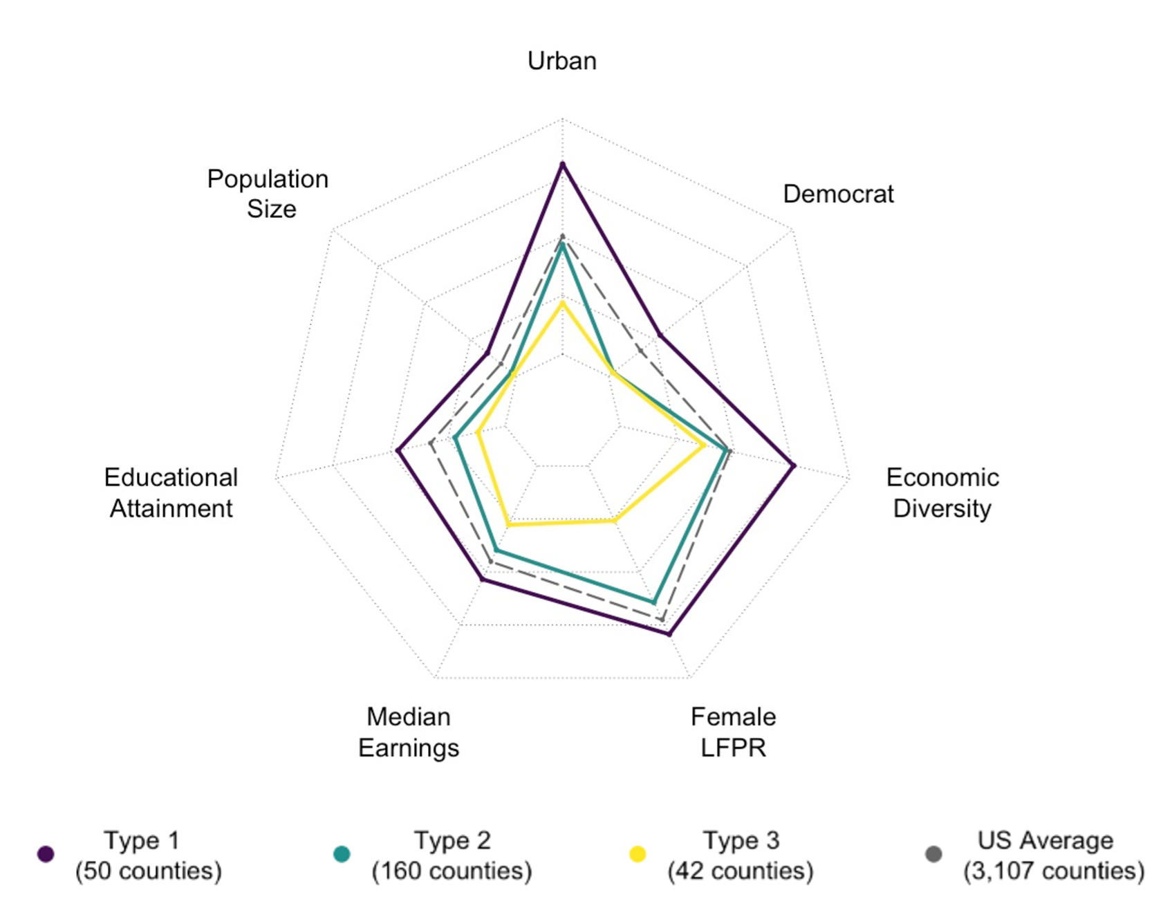
Figure 4: The outer (inner) limit of the radar plot represents the maximum (minimum) value of each characteristic present in the dataset of coal counties. The variable for political affiliation (2016 and 2020 national election returns) is included in this radar plot for illustrative purposes. It is not included in the clustering method as nearly all counties with active coal mines between 2002 and 2019 voted for the Republican Party in the 2016 and 2020 elections. Average values for each indicator per group and the US overall used to generate this plot are reported in detail in Appendix D of the Supplementary Materials.

Figure 4 provides a visual comparison of each county type identified through an application of hierarchical agglomerative clustering on the described set of county characteristics. Figure 4 presents the mean values of each indicator per county type and for the US overall. These mean characteristics are reported in Appendix D of the Supplementary Materials. The geographical distribution of these types is represented in Figure 5.

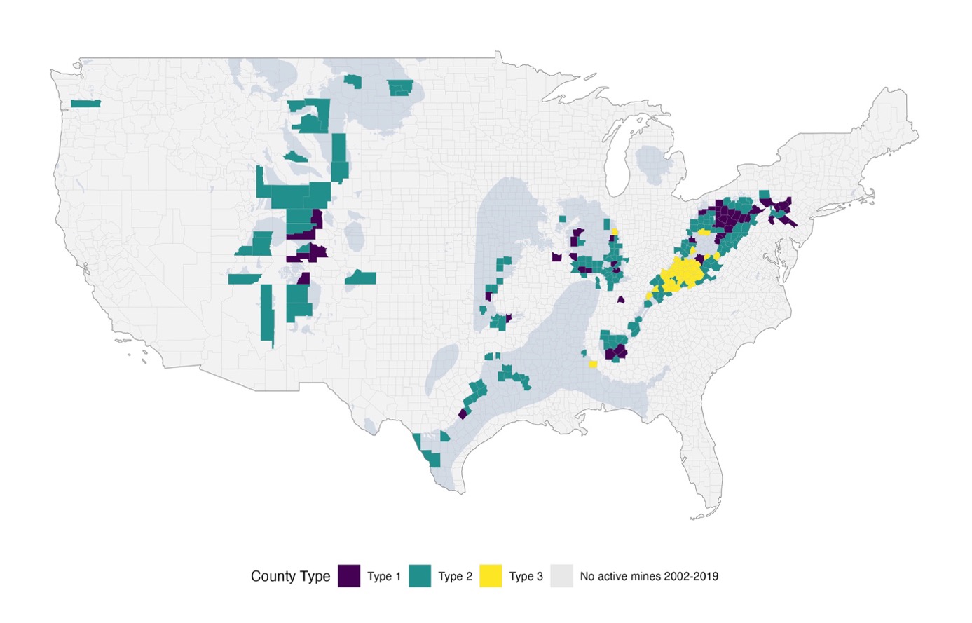
Figure 5: Counties with active coal mines in the period 2002-2019 are color coded according to their “type” as defined by the agglomerative hierarchical clustering performed. Type 1 counties are considered “least vulnerable” due to their relatively stronger performance across the indicators (ie. urban with higher levels of income, educational attainment, economic diversity, female labor force participation, and population), selected in the construction of the typology whereas Type 3 counties are “most vulnerable.” The shaded blue areas represent, from left to right, the Western, Interior, and Appalachian coal basins generated using data available from the US Geological Survey.

The three county “types” fall into a spectrum ranging from large and urban with high levels of educational attainment, income, female labor force participation, and economic diversity (Type 1) to small and rural with lower levels of the subsequent indicators (Type 3). This pattern is perhaps unsurprising to most readers as the economic and social indicators outlined tend to decrease between urban and rural counties. However, one of the more significant results is that Type 3, and to a lesser extent Type 2, coal counties fall well below the national average for all observed indicators that are likely to aid in an eventual transition. Furthermore, Figure 5 demonstrates that Type 3 counties (yellow) are concentrated in the Appalachian coal region, indicating a high risk of regional decline which is already being observed in the area. The fact that Type 3 counties are clustered in one region and share most of their borders with each other or Type 2 counties (apart from one Type 1 county) also indicates a geographical limitation to accessible recovery or transition options should there be a need for laid-off workers migrate.

4.5 Putting the Typology to Work

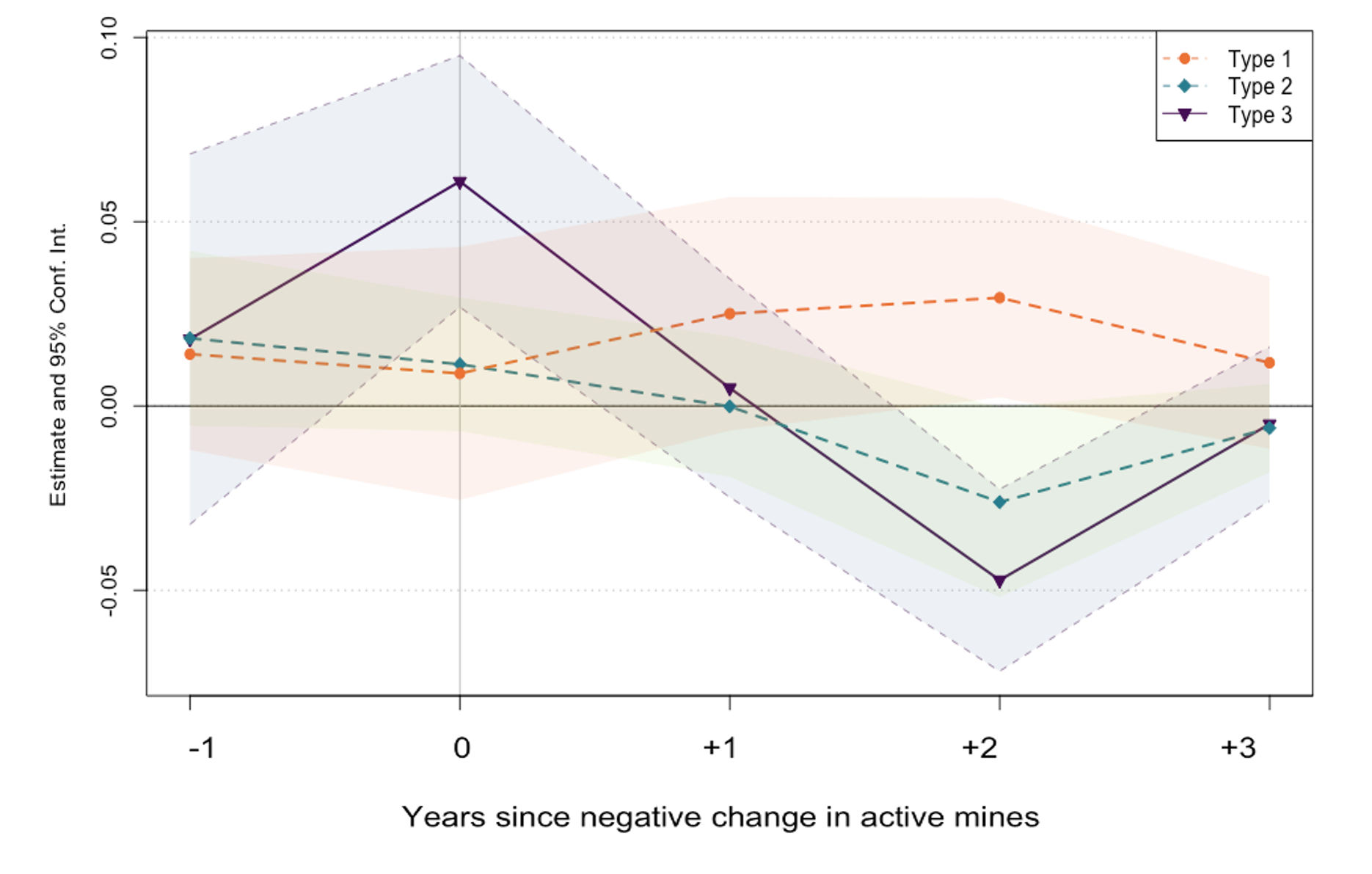
Figure 6: As in Figure 1, Figure 6 presents the change in unemployment rate and associated 95% confidence interval resulting from a change in active mines. The sign of the coefficient estimate has been flipped to demonstrate the impact of a negative change in active mines. Each plotted line and confidence interval represents the response to a change in active mines by county type, as defined in Appendix D.2 in Supplementary Materials.

To put this typology to work, Model 1 was re-estimated using grouped fixed effects, allowing heterogeneous treatment effects for each county type. This enables us to determine whether the scale and duration of unemployment rate responses to changes in active coal mines differ across county types. Figure 6 demonstrates the coefficient estimates across our selected time horizon. Although Model 1 only includes the independent variables listed in Model 1 of Table 1, the additional lags and leads displayed in Figure 6 do not greatly impact the estimates at times t = t, t+1, and t+2 and are therefore included in the visual below for additional information. Regression results from this grouped fixed effects application of Model 1 and expanded one-lead and four-lag models are reported in Appendix D.2 of the Supplementary Materials.

Most notably, Figure 6 illustrates that the greatest unemployment rate increases are observed in Type 3 counties, at a magnitude of 0.060 percentage points (1% significance level) in response to a contemporaneous one-unit decrease in active mines. The coefficient estimates associated with Type 2 and 3 counties are all much smaller in magnitude and not statistically significant.

5 Discussion

In this study, we examine employment shocks in US coal-mining counties undergoing decarbonization-related transitions. We corroborate our results using various panel econometric methods designed to address unobserved heterogeneity and cross-sectional dependence, including TWFE OLS, spatial effects, heterogeneous trends, and grouped fixed effects estimators. We find that a one-unit decline in active mines increases county-level unemployment by between 0.056 to 0.064 percentage points, with little change a year later and a small ‘recovery’ two years later. We further determine that this ‘recovery’ is likely not attributable to a recovery in employment. Given the irreducible element of unpredictability in county unemployment rates, especially in relation to the closure of an often proportionally small sector like coal, it is highly significant that our results show consistent estimates of regression coefficients across all models and reinforces our confidence in using these estimates to guide further reflections on policy responses.

Spatial and heterogeneous trend models show how the TWFE OLS approach underestimates unemployment effects. Incorporating spatial diffusion shows the risk of regional spill-over. Incorporating an asymmetric treatment estimation shows that opening new mines has no obvious influence on unemployment, but mine closures do. This result questions the belief that maintaining or boosting the coal sector will contribute to employment and reveals that mine closures have a stronger impact on unemployment than was initially detected in Model 1. This latter result provides crucial information for improving proposals - such as the one recently proposed by Senator Joe Manchin – to reform federal and state permit approval processes in the mining and energy sectors [28]. In particular, efforts to speed up and streamline permit approval process, as advocated in Manchin’s proposal, would very likely boost green transition mining while also artificially extending the coal sector’s operations beyond what its market outlook and the exigencies of climate change could conceivably permit. As the country awaits the congressional verdict on how the government will balance the trade-offs between issuing fast and efficient energy permitting on the one hand and appropriate environmental impact accounting on the other, future research could investigate how it may be possible to ramp up ’green’ mining of minerals such as copper and silicon – which will be necessary to acquire the raw inputs enabling domestic manufacture of green technologies – while at the same time avoiding continued reliance on coal energy and redeploying, where possible, laid-off coal miners interested in supporting the nation’s next phase of green industrialization [22].

We further evaluated the influence of renewable energy investments on job losses to evaluate claims that green sectoral investments should be the principal means of aiding transitioning coal mining regions. Unfortunately, we were unable to detect significant effects of these investments on county unemployment rates. Determining whether this is due to the lack of a systematic relationship between the two variables or due simply to a lack of sufficiently large investment volumes during the period examined is outside the scope of this study. Nevertheless, we propose ramping up such investments, not only to decarbonize the US economy, but also to enhance the potentialities of new employment in coal counties with already low economic diversification. In certain localities, such initiatives have been beneficial, and the Inflation Reduction Act is encouraging on that front, even though it ignores the likely utility of other complimentary policy measures [34].

Lastly, the typology offered in this paper reveals that most coal counties are slated to experience outsized socio-economic struggles following large-scale decarbonization compared to the nation’s average performance across selected parameters. Empirical research shows that Type 3 counties, mostly in Appalachia, are the most heavily impacted. Most transitional assistance and social reconstruction efforts should focus on these counties.

These findings provide information crucial for making policy prescriptions since they enable better consideration of the specific needs of communities most impacted. First, low educational attainment and female labour force participation in Type 2 and 3 counties underscore the need for reskilling, retraining, and subsidized community college or vocational training for women. Subsidized day-care and after-school programs will be required so parents may attend these trainings after work. Second, the low level of economic diversity in Type 2 and 3 counties may hinder investment in other sectors. Investments that counteract Type 2 and 3 counties’ poor economic diversity therefore ought to be considered alongside active labour market policies. Public subsidies may be needed to stimulate investment in low-diversity areas. The IRA’s proposed reinvestment in energy infrastructure looks wise in this respect. Future research can investigate which policy instruments would most effectively mitigate against avoidable socio-economic and psychological hardship in places ”left behind” due to bad investment conditions and low economic diversity.

Interestingly, even in Type 3 counties, median incomes are near the national average, so direct income support may not be the greatest use of public or private funds. However, income support to cover health care costs could be necessary during lapses in insurance, a claim demanded by the United Mine Workers of America (UMWA) [67].

Our econometric analysis indicates that the greatest policy difficulty may not be a time-persistent unemployment shock but rather its spatial ripple effect. The rural-urban split between Type 2 and 3 counties and Type 1 counties would likely require substantial inter-regional mobility or transportation upgrades to help laid-off workers find new jobs. Due to the preponderance of Type 3 counties, Appalachia will likely have the highest investment costs. In severe cases, relocation support should be explored for unemployed workers in rural areas with minimal economic diversity and wherever inter-regional transit is extremely expensive or impossible.

A main risk of a poorly managed transition is the potential to erode support for future environmental action. Recent research on popular acceptance of environmental measures in the US indicates that environmental policy bundled with social safeguards might boost public support, offering further grounds for the social and political practicality of a Just Transition agenda [49, 10]. Incorporating Just Transition concepts into decarbonization policies may boost support for environmental programmes generally. The UMWA seems to reflect this sentiment, as it has expressed a willingness to embrace a green transition provided that affected workers are supported along the way [20].

Finally, to the disservice of US communities still struggling with the effects of coal’s decline, the ’situation’ of US coal employees is increasingly being used as an example of failed Just Transition aspirations, with academic researchers and public commentators asking how the transition from oil and gas might avoid similar issues. This study reiterates that coal communities deserve sustained attention while also outlining a framework of inquiry that could inform future research focusing on unemployment shocks following oil and gas sector decarbonization.

6 Conclusion

The research presented herein is crucial because it elucidates the immediate effects of mine closures on coal communities and demonstrates the urgent requirement for transition support following an unemployment shock caused by decarbonization. Coal-dependent counties are typically rural areas with limited economic opportunities, low rates of female labour force participation, and low levels of educational attainment. Policies that aim to counteract the transitional risks, vulnerabilities, and hardships experienced in these disproportionately affected communities can achieve maximum effectiveness provided they are strategically targeted and sufficiently farsighted to minimise the geographic spill-over of negative repercussions. This research has paved the way for the development of empirically grounded, context-dependent ameliorative strategies. This research has also shed light on how the provisions of the recently enacted Inflation Reduction Act might benefit communities that rely on fossil fuels, showing that while smarter green economy investment targeting could help these communities weather the inevitable green transition, broader and more concerted policy provisions are needed to ensure a Just Transition.

7 Supplementary Materials

Appendix A Summary Statistics and Data Sources

A.1 Econometric Models

Table S2: Indicators and Data Sources

Indicator	Data Source	Survey/Dataset
Population	US Department of Commerce	Local Area Personal Income
	Bureau of Economic Analysis (BEA)	and Employment Statistics
Labour Force		Local Area
Employed Persons	US Bureau of Labor Statistics (BLS)	Unemployment Statistics
Unemployed Persons
Unemployment Rate
Active mines	US Energy Information Administration (EIA)	Mine Employment and
	and the US Mine Safety and Health	Coal Production Data
	Administration (MSHA)
Renewable Energy	US Department of Agriculture	Energy Investment Report
Investments
County Adjacency Matrix	US Census Bureau	County Adjacency File

Table S3: Summary Statistics: Contiguous US Counties

Statistic	N	Mean	St. Dev.	Min	Pctl(25)	Pctl(75)	Max
Active Mines	55,296	0.462	3.723	0	0	0	114
Unemployment Rate	55,296	6.130	2.720	0.800	4.200	7.500	29.400
Employed Persons	55,296	46,504	149,661	34	4,799	30,140	4,888,581
Unemployed Persons	55,296	2,993	11,183	3	293	1,988	621,950
Labour Force	55,296	49,498	159,938	38	5,128	32,055	5,122,843
Population	55,296	99,440	318,828	55	11,223	67,553	10,105,708
RE Investments (USD)*	55,296	114,142	2,670,894	0	0	0	250,000,000
Real GDP	55,296	5,140,646	22,046,739	7,648	342,473	2,550,861	726,943,301
Real GDP Per Capita	55,296	50.84	463.90	5.79	25.90	46.76	59,848.92
Rural-Urban Code	55,296	5.1	2.7	1	3	7	9
Rural-Urban (binary)	55,296	0.65	0.48	0	0	1	1
RE Inv. (prop. of Real GDP)**	55,296	0.091	3.073	0	0	0	504

*RE Investments (USD): Level of renewable energy investment in US dollars.
*RE Inv. (prop. of Real GDP): Level of renewable energy investment as proportion of county real GDP.

Table S4: Summary Statistics: US Coal Counties

Statistic	N	Mean	St. Dev.	Min	Pctl(25)	Pctl(75)	Max
Active Mines	4,518	5.653	11.847	0	1	5	114
Unemployment Rate	4,518	6.946	2.520	2	5.2	8.3	21
Employed Persons	4,518	29,070	58,839	816	6,859	27,426	622,714
Unemployed Persons	4,518	1,933	3,535	32	477	1,890	46,564
Labour Force	4,518	31,003	62,187	870	7,392	29,621	651,926
Population	4,518	64,867	119,766	1,836	16,721	64,537	1,265,577
RE Investments (USD)*	4,518	27,056	333,440	0	0	0	10,005,017
Coal Production (short tons)	4,518	4,057,556	22,253,668	0	0	3,564,906	415,924,096
Real GDP	4,518	3,045,039	7,913,160	47,597	590,750	2,623,148	92,984,370
Real GDP Per Capita	4,518	41.688	25.763	8.221	26.348	48.551	244.161
Rural-Urban Code	4,518	5.116	2.376	1	3	7	9
Rural-Urban (binary)	4,518	0.697	0.460	0	0	1	1
TAA Allocation (USD)	4,518	14,597,789	20,533,595	0	0	23,427,230	117,476,517
RE Inv. (prop. of Real GDP)**	4,518	0.016	0.241	0	0	0	9

Table S5: Summary Statistics of Transformed Variables: Contiguous US Counties

Statistic	N	Mean	St. Dev.	Min	Pctl(25)	Pctl(75)	Max
$\Delta$ Unemployment Rate	55,296	$-$0.061	1.228	$-$8.600	$-$0.700	0.300	13.500
$\Delta$ Active Minest	55,296	$-$0.015	0.605	$-$30	0	0	20
$\Delta$ (log) Real GDP	55,295	0.017	0.088	$-$1.122	$-$0.017	0.048	1.386
$\Delta$ (log) Real GDP per capita	55,295	0.014	0.088	$-$1.126	$-$0.020	0.043	1.391
$\Delta$ (log) Employed Persons	55,296	0.001	0.037	$-$0.596	$-$0.013	0.018	1.022
$\Delta$ (log) Unemployed Persons	55,296	$-$0.013	0.177	$-$0.852	$-$0.124	0.057	1.305
$\Delta$ (log) Labour Force	55,296	0.001	0.034	$-$0.562	$-$0.013	0.015	0.986
$\Delta$ (log) Population	55,295	0.003	0.014	$-$0.425	$-$0.005	0.009	0.290
REE $\geq 0.1$% of GDP	55,296	0.127	0.333	0	0	0	1

Table S6: Summary Statistics of Transformed Variables: US Coal Counties Subset

Statistic	N	Mean	St. Dev.	Min	Pctl(25)	Pctl(75)	Max
$\Delta$ Unemployment Rate	4,518	$-$0.056	1.322	$-$4.600	$-$0.793	0.400	8.300
$\Delta$ Active Minest	4,518	$-$0.182	2.109	$-$30	0	0	20
$\Delta$ (log) Real GDP	4,518	0.010	0.081	$-$0.604	$-$0.022	0.038	1.342
$\Delta$ (log) Real GDP per capita	4,518	0.010	0.080	$-$0.594	$-$0.021	0.037	1.351
$\Delta$ (log) Employed Persons	4,518	$-$0.002	0.035	$-$0.440	$-$0.015	0.014	0.214
$\Delta$ (log) Unemployed Persons	4,518	$-$0.014	0.179	$-$0.479	$-$0.120	0.051	1.077
$\Delta$ (log) Labour Force	4,518	$-$0.003	0.031	$-$0.396	$-$0.015	0.012	0.185
$\Delta$ (log) Population	4,518	$-$0.0004	0.010	$-$0.098	$-$0.006	0.004	0.066
REE $\geq 0.1$% of GDP	4,518	0.097	0.296	0	0	0	1

A.2 Typology

Table S7: Indicators and Data Sources

Characteristic	Indicator	Data Source	Survey/Dataset
Rural vs. Urban	Rural-Urban Codes	US Department of	Rural-Urban Continuum
		Agriculture’s Economic	Codes 2013
		Research Service
Population Size	2019 Population Estimate	US Census Bureau	Population and Housing
			Unit Estimates
Educational	Percentage of population	US Census Bureau	American Community Survey
Attainment	aged 25-64 with at least
	a bachelor’s degree
Economic Security	Median earnings (USD)	US Census Bureau	American Community Survey
Female Labor	Labor force participation rate	US Census Bureau	American Community Survey
Force Participation	of the female population
Rate	aged 25-64 years
Economic Diversity	Economic Diversity Index	Chmura Economics	Economic Diversity Index
		and Analytics
Political Attitudes	2016 and 2020	MIT Election Data	County Presidential
	Election Returns	and Science Lab	Election Returns 2000-2020

Typology: Motivation for Indicator Choices

Summary: County demographic, social, economic, and political characteristics that have previously been identified as having potential to affect or determine an area’s ability or potential to transition smoothly during and after and economic shift or shock were collected.

Rural vs. Urban: First, whether a county is more urban or rural can affect the proximity of newly unemployed workers formerly in brown industries to other job and education opportunities but will also impact identity construction surrounding extractive industries and limit accessibility to policymakers and other resources intended to support achieving a Just Transition.

Population Size: Second, population size is an important predictor of political reach and voice as well as economic activity and opportunities.

Educational Attainment: Third, the average level of educational attainment will impact qualifications and skill levels of individuals looking for new job opportunities, particularly in the face of a potential skills-biased structural decarbonization. This may be of particular concern in resource-rich regions, as job opportunities presented in extractive industries and natural resource production have been found to provide a disincentive to education, especially among young men.

Economic Security: Next, median earnings was used to proxy the level of economic security of a county. A lower level of economic security can imply great hardship for individuals and households facing periods of unemployment without savings to fall back on.

Female Labor Force Participation Rate: Next, the coal mining industry, much like the fossil fuel industry overall, has a largely male-dominated workforce meaning the prospect of lay-offs of a male-dominated workforce will leave many households reliant on the income or labor of females. Therefore, boosting female employment in other industries might provide crucial income support during periods of transition for the implicated partners. This effect is proxied in the typology by female labor force participation among women between 25 and 64 years of age.

Economic Diversity: Furthermore, economic diversity, or the mix of industries providing employment within a county, is an important determinant not only of the proximate available job opportunities for workers to transition into but also potential sites of investment to boost economic opportunities, whether green or otherwise.

Political Attitudes: Lastly, political attitudes or party affiliation will dictate the type of messaging surrounding transitions that will either corrode or boost public support and willingness to engage with implemented support measures. Furthermore, as ambitions relating to environmental regulation as well as investments in renewable energy and energy efficiency industries are generally advanced by the US Democratic party, political party affiliation will likely dictate the kinds of opportunities that will be created for fossil fuel workers facing unemployment risks. Originally, political attitudes were intended to be proxied by county returns in the 2016 and 2020 presidential elections. However, only 19 of 252 coal counties voted for the Democratic party in the 2016 and 2020 presidential elections and this was therefore excluded from the clustering analysis as Republican party affiliation seems to be a unifying characteristic among coal counties.

Table S8: Summary Statistics: Stylized Typology Characteristics

Statistic	N*	Mean	St. Dev.	Min	Pctl(25)	Pctl(75)	Max
2013 Rural-Urban Code	252	5.1	2.4	1	3	7	9
Population Size	252	64,655.3	121,468.2	1,959	16,684.5	64,320.2	1,216,045
Educational Attainment	252	18.2	7.7	5.4	13.6	20.7	56.2
(%; aged 25-64)
Median Earnings (USD)	252	34,204.2	4,935.0	20,268	31,357	36,705.2	54,754
Female Labour Force Participation	252	64.6	8.9	37.9	60.3	71.1	81.7
(%; aged 25-64)
Chmura Diversity Index	252	1.0	0.2	0.5	0.9	1.1	1.5
Voted for the Republican	252	0.9	0.3	0	1	1	1
Party in the 2020 Election
Voted for the Republican	252	0.9	0.3	0	1	1	1
Party in the 2016 Election

Note: The state of Virginia’s counties are measured differently across data sources. More precisely, the BEA combines independent cities of Virginia with adjacent counties thus reporting less county observations than in the remaining data sources. For the econometric applications, this discrepancy was overcome by adjusting the remaining data sources to match the county identification codes provided by the BEA. Conventional FIPS codes were used for the typology analysis to allow for the inclusion of the relevant indicators with minimal additional manipulation. Only one county retained in the typology analysis is implicated in the BEA-Census Bureau discrepancy, thus the impact of this choice on the results is deemed minimal. Therefore, in the subsequent analysis, econometric applications make use of 3,072 county observations versus the 3,107 counties observed in the typology dataset. Additionally, for the subset of coal counties, the number of counties included in the typology (252) differs from the number identified in the econometric analysis (251) because Wise County, Virginia and Norton City, Virginia are considered separately by the various entities reporting data for the typology characteristics. They are combined into one county area by the Bureau of Economic Analysis whose method was adopted as the standard for the econometric analysis.

Alaska, Hawaii, and the District of Columbia (DC) were excluded from the analysis. Hawaii does not produce coal. Indicators for DC are inconsistently reported across the datasets involved in this analysis. During the 18-year time period analyzed, Alaska’s county equivalents were divided and re-grouped making it difficult to compare available data between time periods. The exclusion of DC is considered a limitation in this work.

Appendix B Econometric Models

B.1 Two-way fixed effects (TWFE) OLS models

B.1.1 Level indicators

Table S9: Impact of the number of active mines on county unemployment rate (level)
Using a TWFE OLS regression model with various combinations of time lags and leads

Dependent Variable:	Unemployment Rate
Model:	(1)	(2)	(3)	(4)	(5)	(6)
	All US Counties			Coal Counties Only
Variables
Active Minest+3			-0.0284.			-0.0177
			(0.0134)			(0.0116)
Active Minest+2		-0.0293∗	-0.0030		-0.0220.	-0.0059
		(0.0127)	(0.0033)		(0.0115)	(0.0042)
Active Minest+1		-0.0164	-0.0150		-0.0173	-0.0168
		(0.0150)	(0.0138)		(0.0137)	(0.0131)
Active Mines	-0.0938∗∗∗	-0.0585∗	-0.0620∗∗	-0.0740∗∗∗	-0.0446∗	-0.0468∗
	(0.0202)	(0.0206)	(0.0187)	(0.0178)	(0.0172)	(0.0161)
Active Minest-1	-0.0051	-0.0053	-0.0084	-0.0046	-0.0055	-0.0085
	(0.0159)	(0.0115)	(0.0105)	(0.0143)	(0.0103)	(0.0095)
Active Minest-2	0.0425∗∗∗	0.0456∗∗∗	0.0353∗∗∗	0.0360∗∗∗	0.0404∗∗∗	0.0306∗∗∗
	(0.0106)	(0.0090)	(0.0056)	(0.0091)	(0.0089)	(0.0041)
Active Minest-3	0.0259∗		0.0059	0.0227∗		0.0074
	(0.0102)		(0.0093)	(0.0099)		(0.0090)
(log) Real GDPPCt	-0.9987∗∗	-1.283∗∗∗	-1.473∗∗∗	-1.118∗∗∗	-1.367∗∗∗	-1.542∗∗∗
	(0.2558)	(0.3114)	(0.3444)	(0.2559)	(0.2884)	(0.3149)
Fixed-effects
County FIPS Code	Yes	Yes	Yes	Yes	Yes	Yes
Year	Yes	Yes	Yes	Yes	Yes	Yes
Fit statistics
Observations	55,296	49,152	46,080	4,518	4,016	3,765
R2	0.84475	0.84904	0.85296	0.85387	0.85524	0.85904
Within R2	0.02682	0.04056	0.04970	0.09054	0.12315	0.13941
Clustered (County FIPS Code & Year) standard-errors in parentheses
Signif. Codes: ***: 0.001, **: 0.01, *: 0.05, .: 0.1

Table S10: Impact of the number of active mines on county employment indicators (levels)
Using a TWFE OLS regression model with two time lags on all contiguous US counties

Dependent Variables:	Employed	Unemployed	Labour	Population
	Persons	Persons	Force
Model:	(1)	(2)	(3)	(4)
Variables
Active Mines	12.69	-1.205	11.48	206.3∗
	(31.64)	(8.444)	(25.46)	(88.22)
Active Mines (t-1)	5.954	-10.81	-4.855	3.627
	(35.37)	(9.848)	(25.96)	(71.04)
Active Mines (t-2)	-26.95	-16.02	-42.97	48.69
	(31.95)	(10.33)	(26.05)	(60.87)
(log) Real GDPt	1,939.9∗	-659.7∗∗	1,280.2.	8,575.3∗∗∗
	(679.6)	(209.3)	(633.7)	(2,153.9)
(log) Populationt	62,741.2∗∗∗	1,230.3	63,971.5∗∗∗
	(6,328.0)	(1,867.3)	(5,602.1)
Fixed-effects
County FIPS Code	Yes	Yes	Yes	Yes
Year	Yes	Yes	Yes	Yes
Fit statistics
Observations	55,296	55,296	55,296	55,296
R2	0.99619	0.89335	0.99714	0.99684
Within R2	0.10605	0.00097	0.12340	0.00619
Clustered (County FIPS Code & Year) standard-errors in parentheses
Signif. Codes: ***: 0.001, **: 0.01, *: 0.05, .: 0.1

Table S11: Impact of the number of active mines on county employment indicators (log levels excl. UER)
Using a TWFE OLS regression model with two time lags on all contiguous US counties

Dependent Variables:	Unemployment	Employed	Unemployed	Labour	Population
	Rate	Persons (log)	Persons (log)	Force (log)	(log)
Model:	(1)	(2)	(3)	(4)	(5)
Variables
Active Mines	-0.0955∗∗∗	0.0015∗	-0.0103∗∗∗	0.0004	0.0012
	(0.0205)	(0.0006)	(0.0020)	(0.0006)	(0.0007)
Active Minest-1	-0.0035	0.0012.	$-9.24\times 10^{-5}$	0.0012	0.0003
	(0.0157)	(0.0007)	(0.0015)	(0.0007)	(0.0007)
Active Minest-2	0.0619∗∗∗	-0.0005	0.0040∗	0.0002	0.0010
	(0.0122)	(0.0004)	(0.0015)	(0.0005)	(0.0007)
(log) Real GDPPCt	-0.9989∗∗
	(0.2558)
(log) Real GDPt		0.1035∗∗∗	-0.0926∗∗	0.0929∗∗∗	0.0665∗∗∗
		(0.0106)	(0.0300)	(0.0099)	(0.0110)
(log) Populationt		0.9033∗∗∗	1.103∗∗∗	0.9189∗∗∗
		(0.0298)	(0.0878)	(0.0287)
Fixed-effects
County FIPS Code	Yes	Yes	Yes	Yes	Yes
Year	Yes	Yes	Yes	Yes	Yes
Fit statistics
Observations	55,296	55,296	55,296	55,296	55,296
R2	0.84472	0.99857	0.99204	0.99876	0.99891
Within R2	0.02664	0.45766	0.12865	0.49102	0.05022
Clustered (County FIPS Code & Year) standard-errors in parentheses
Signif. Codes: ***: 0.001, **: 0.01, *: 0.05, .: 0.1

Table S12: Impact of a change in active mines on county employment indicators (log levels excl. unemployment rate)
Using a TWFE OLS regression model on all contiguous US counties

Dependent Variables:	Unemployment	Employed	Unemployed	Labour	Population
	Rate	Persons (log)	Persons (log)	Force (log)	(log)
Model:	(1)	(2)	(3)	(4)	(5)
Variables
$\Delta$ Active Minest	-0.0835∗∗∗	0.0007	-0.0081∗∗∗	-0.0002	0.0003
	(0.0198)	(0.0006)	(0.0020)	(0.0007)	(0.0008)
$\Delta$ Active Minest-1	-0.0884∗∗∗	0.0020∗∗	-0.0082∗∗∗	0.0010.	0.0006
	(0.0148)	(0.0005)	(0.0020)	(0.0005)	(0.0008)
$\Delta$ Active Minest-2	-0.0446∗∗	0.0021∗∗∗	-0.0044.	0.0016∗∗∗	0.0009
	(0.0149)	(0.0005)	(0.0021)	(0.0004)	(0.0007)
(log) Real GDPPCt	-1.011∗∗∗
	(0.2531)
(log) Real GDPt		0.1044∗∗∗	-0.0955∗∗	0.0937∗∗∗	0.0679∗∗∗
		(0.0105)	(0.0294)	(0.0098)	(0.0112)
(log) Populationt		0.9051∗∗∗	1.097∗∗∗	0.9203∗∗∗
		(0.0302)	(0.0887)	(0.0290)
Fixed-effects
County FIPS Code	Yes	Yes	Yes	Yes	Yes
Year	Yes	Yes	Yes	Yes	Yes
Fit statistics
Observations	55,296	55,296	55,296	55,296	55,296
R2	0.84465	0.99857	0.99203	0.99876	0.99891
Within R2	0.02622	0.45720	0.12733	0.49067	0.04813
Clustered (County FIPS Code & Year) standard-errors in parentheses
Signif. Codes: ***: 0.001, **: 0.01, *: 0.05, .: 0.1

B.1.2 First-difference indicators

Table S13: Impact of change in active mines on the change in unemployment rate
Using a TWFE OLS regression model on all contiguous counties and coal counties with various combinations of time lags and leads

Dependent Variable:	$\Delta$ Unemployment Rate
Model:	(1)	(2)	(3)	(4)	(5)	(6)
	All US Counties			Coal Counties Only
Variables
$\Delta$ Active Minest+3			-0.0186∗			-0.0087
			(0.0082)			(0.0080)
$\Delta$ Active Minest+2		-0.0050	-0.0056		-0.0068	-0.0065
		(0.0112)	(0.0128)		(0.0084)	(0.0097)
$\Delta$ Active Minest+1		-0.0203	-0.0168		-0.0201	-0.0169
		(0.0206)	(0.0184)		(0.0182)	(0.0170)
$\Delta$ Active Minest	-0.0562∗∗	-0.0588∗∗∗	-0.0587∗∗∗	-0.0410∗∗	-0.0441∗∗	-0.0427∗∗
	(0.0142)	(0.0142)	(0.0138)	(0.0124)	(0.0127)	(0.0127)
$\Delta$ Active Minest-1	-0.0070	-0.0083	-0.0138	-0.0040	-0.0062	-0.0094
	(0.0138)	(0.0158)	(0.0160)	(0.0100)	(0.0118)	(0.0124)
$\Delta$ Active Minest-2	0.0391∗∗	0.0388∗	0.0274.	0.0343∗∗	0.0333∗∗	0.0264∗
	(0.0131)	(0.0137)	(0.0139)	(0.0106)	(0.0111)	(0.0123)
$\Delta$ Active Minest-3	0.0013		-0.0078	0.0036		-0.0026
	(0.0104)		(0.0099)	(0.0074)		(0.0078)
$\Delta$ (log) Real GDPPCt	-0.9738∗∗∗	-0.9937∗∗∗	-1.025∗∗∗	-1.587∗∗∗	-1.611∗∗∗	-1.647∗∗∗
	(0.2137)	(0.2181)	(0.2177)	(0.3505)	(0.3667)	(0.3715)
Fixed-effects
County FIPS Code	Yes	Yes	Yes	Yes	Yes	Yes
Year	Yes	Yes	Yes	Yes	Yes	Yes
Fit statistics
Observations	55,295	49,151	46,079	4,518	4,016	3,765
R2	0.61338	0.61965	0.62238	0.65489	0.66562	0.67289
Within R2	0.01470	0.01532	0.01530	0.04548	0.05083	0.04918
Clustered (County FIPS Code & Year) standard-errors in parentheses
Signif. Codes: ***: 0.001, **: 0.01, *: 0.05, .: 0.1

Table S14: Impact of change in active mines on the change in county employment indicators (log excl. UER)
Using a TWFE OLS regression model on all contiguous US counties

Dependent Variables:	$\Delta$ Unemployment	$\Delta$ Employed	$\Delta$ Unemployed	$\Delta$ Labour	$\Delta$ Population
	Rate	Persons (log)	Persons (log)	Force (log)	(log)
Model:	(1)	(2)	(3)	(4)	(5)
Variables
$\Delta$ Active Minest	-0.0563∗∗∗	0.0011∗	-0.0055∗∗	0.0005	$-4.5\times 10^{-5}$
	(0.0141)	(0.0004)	(0.0016)	(0.0003)	($7.38\times 10^{-5}$)
$\Delta$ Active Minest-1	-0.0070	0.0016∗∗∗	-0.0003	0.0016∗∗∗	0.0001
	(0.0136)	(0.0003)	(0.0014)	(0.0003)	($6.61\times 10^{-5}$)
$\Delta$ Active Minest-2	0.0389∗∗	0.0004	0.0036.	0.0009.	0.0002∗
	(0.0125)	(0.0004)	(0.0018)	(0.0004)	($7.04\times 10^{-5}$)
$\Delta$ (log)Real GDPPCt	-0.9738∗∗∗
	(0.2137)
$\Delta$ (log)Real GDPt		0.0514∗∗∗	-0.1025∗∗∗	0.0409∗∗∗	0.0076∗∗∗
		(0.0067)	(0.0196)	(0.0051)	(0.0016)
$\Delta$ (log)Populationt		0.5302∗∗∗	0.9293∗∗∗	0.5543∗∗∗
		(0.0634)	(0.1869)	(0.0598)
Fixed-effects
County FIPS Code	Yes	Yes	Yes	Yes	Yes
Year	Yes	Yes	Yes	Yes	Yes
Fit statistics
Observations	55,295	55,295	55,295	55,295	55,295
R2	0.61338	0.20841	0.65143	0.18310	0.44840
Within R2	0.01470	0.04780	0.01637	0.05150	0.00377
Clustered (County FIPS Code & Year) standard-errors in parentheses
Signif. Codes: ***: 0.001, **: 0.01, *: 0.05, .: 0.1

Table S15: Impact of change in active mines on changes in county employment indicators (log excl. UER)
Using a TWFE OLS regression model on US coal counties

Dependent Variables:	$\Delta$ Unemployment	$\Delta$ Employed	$\Delta$ Unemployed	$\Delta$ Labour	$\Delta$ Population
	Rate	Persons (log)	Persons (log)	Force (log)	(log)
Model:	(1)	(2)	(3)	(4)	(5)
Variables
$\Delta$ Active Minest	-0.0413∗∗	0.0008.	-0.0037∗	0.0003	$-4.21\times 10^{-5}$
	(0.0124)	(0.0004)	(0.0013)	(0.0003)	($5.96\times 10^{-5}$)
$\Delta$ Active Minest-1	-0.0042	0.0013∗∗∗	0.0002	0.0013∗∗∗	$5.8\times 10^{-5}$
	(0.0099)	(0.0003)	(0.0010)	(0.0003)	($6.04\times 10^{-5}$)
$\Delta$ Active Minest-2	0.0338∗∗	0.0004	0.0035∗	0.0008∗	0.0001∗
	(0.0101)	(0.0004)	(0.0015)	(0.0004)	($5.54\times 10^{-5}$)
$\Delta$ (log)Real GDPPCt	-1.588∗∗∗
	(0.3504)
$\Delta$ (log)Real GDPt		0.0650∗∗∗	-0.1615∗∗	0.0473∗∗∗	0.0054.
		(0.0122)	(0.0409)	(0.0102)	(0.0027)
$\Delta$ (log)Populationt		0.7066∗∗∗	1.046	0.7134∗∗∗
		(0.1054)	(0.6443)	(0.0938)
Fixed-effects
County FIPS Code	Yes	Yes	Yes	Yes	Yes
Year	Yes	Yes	Yes	Yes	Yes
Fit statistics
Observations	4,518	4,518	4,518	4,518	4,518
R2	0.65485	0.25173	0.68570	0.22373	0.49417
Within R2	0.04538	0.06787	0.03124	0.06505	0.00538
Clustered (County FIPS Code & Year) standard-errors in parentheses
Signif. Codes: ***: 0.001, **: 0.01, *: 0.05, .: 0.1

Table S16: Impact of change in active mines in various time periods on the change in unemployment rate
Using a TWFE OLS regression model on all contiguous counties and coal counties using single time periods

Dependent Variable:	$\Delta$ Unemployment Rate
Model:	(1)	(2)	(3)	(4)	(5)	(6)	(7)	(8)
Variables
$\Delta$ Active Minest	-0.0560∗∗				-0.0416∗∗
	(0.0151)				(0.0127)
$\Delta$ Active Minest-1		-0.0050				-0.0029
		(0.0137)				(0.0096)
$\Delta$ Active Minest-2			0.0402∗				0.0351∗∗
			(0.0151)				(0.0116)
$\Delta$ Active Minest-3				0.0011				0.0026
				(0.0136)				(0.0098)
$\Delta$ (log)Real GDPPCt	-0.9742∗∗∗	-0.9837∗∗∗	-0.9846∗∗∗	-0.9842∗∗∗	-1.596∗∗∗	-1.699∗∗∗	-1.701∗∗∗	-1.702∗∗∗
	(0.2137)	(0.2137)	(0.2138)	(0.2136)	(0.3513)	(0.3482)	(0.3416)	(0.3469)
Fixed-effects
County FIPS Code	Yes	Yes	Yes	Yes	Yes	Yes	Yes	Yes
Year	Yes	Yes	Yes	Yes	Yes	Yes	Yes	Yes
Fit statistics
Observations	55,295	55,295	55,295	55,295	4,518	4,518	4,518	4,518
R2	0.61298	0.61227	0.61267	0.61226	0.65184	0.64795	0.65105	0.64794
Within R2	0.01367	0.01186	0.01288	0.01185	0.03705	0.02628	0.03487	0.02627
Clustered (County FIPS Code & Year) standard-errors in parentheses
Signif. Codes: ***: 0.001, **: 0.01, *: 0.05, .: 0.1

Table S17: Impact of change in active mines on change in unemployment rate
Using a TWFE OLS regression model and binary interaction term for whether a county is rural or not (Rural = 1; Non-rural = 0)

Dependent Variable:	$\Delta$ Unemployment Rate
Model:	(1)	(2)
Variables
$\Delta$ Active Minest	-0.0308∗	-0.0119
	(0.0135)	(0.0134)
$\Delta$ Active Minest-1	-0.0371∗	-0.0306.
	(0.0163)	(0.0160)
$\Delta$ Active Minest-2	0.0027	-0.0039
	(0.0144)	(0.0140)
$\Delta$ (log) Real GDPPCt	-0.9736∗∗∗	-1.583∗∗∗
	(0.2137)	(0.3493)
$\Delta$ Active Mines $\times$ Rural	-0.0288	-0.0335
	(0.0218)	(0.0221)
$\Delta$ Active Minest-1 $\times$ Rural	0.0346	0.0301
	(0.0237)	(0.0238)
$\Delta$ Active Minest-2 $\times$ Rural	0.0420∗	0.0435∗
	(0.0152)	(0.0172)
Fixed-effects
County FIPS Code	Yes	Yes
Year	Yes	Yes
Fit statistics
Observations	55,295	4,518
R2	0.61349	0.65598
Within R2	0.01496	0.04851
Clustered (County FIPS Code & Year) standard-errors in parentheses
Signif. Codes: ***: 0.001, **: 0.01, *: 0.05, .: 0.1

Table S18: Asymmetric treatment on all US counties

Performed using a TWFE OLS regression on all contiguous US counties. Dependent Variable: $\Delta$ Unemployment Rate Model: (1) (2) (3) Variables $\Delta$ Active Mines_t -0.0193 -0.0752^∗∗ (0.0201) (0.0235) $\Delta$ Active Mines_t-1 0.0221 -0.0301 (0.0285) (0.0219) $\Delta$ Active Mines_t-2 0.0090 0.0546^∗∗∗ (0.0236) (0.0116) $\Delta$ (log) Real GDPPC_t -0.9724^∗∗∗ -0.9724^∗∗∗ -0.9724^∗∗∗ (0.2138) (0.2138) (0.2138) $\Delta$ Active Mines_t $\times$ $\Delta_{negative_{t}}$ -0.0559 -0.0752^∗∗ (0.0370) (0.0235) $\Delta$ Active Mines_t-1 $\times$ $\Delta_{negative_{t-1}}$ -0.0521 -0.0301 (0.0422) (0.0219) $\Delta$ Active Mines_t-2 $\times$ $\Delta_{negative_{t-2}}$ 0.0457 0.0546^∗∗∗ (0.0277) (0.0116) $\Delta$ Active Mines_t $\times$ $\Delta_{positive_{t}}$ 0.0559 -0.0193 (0.0370) (0.0201) $\Delta$ Active Mines_t-1 $\times$ $\Delta_{positive_{t-1}}$ 0.0521 0.0221 (0.0422) (0.0285) $\Delta$ Active Mines_t-2 $\times$ $\Delta_{positive_{t-2}}$ -0.0457 0.0090 (0.0277) (0.0236) Fixed-effects County FIPS Code Yes Yes Yes Year Yes Yes Yes Fit statistics Observations 55,295 55,295 55,295 R² 0.61355 0.61355 0.61355 Within R² 0.01513 0.01513 0.01513 Clustered (County FIPS Code & Year) standard-errors in parentheses Signif. Codes: ***: 0.001, **: 0.01, *: 0.05, .: 0.1

Table S19: Asymmetric treatment on subset of US coal counties

Performed using a TWFE OLS regression on US coal counties. Dependent Variable: Change Unemployment Rate Model: (1) (2) (3) Variables $\Delta$ Active Mines_t -0.0193 -0.0752^∗∗ (0.0201) (0.0235) $\Delta$Active Mines_t-1 0.0221 -0.0301 (0.0285) (0.0219) $\Delta$Active Mines_t-2 0.0090 0.0546^∗∗∗ (0.0236) (0.0116) $\Delta$ (log) Real GDPPC_t -0.9724^∗∗∗ -0.9724^∗∗∗ -0.9724^∗∗∗ (0.2138) (0.2138) (0.2138) $\Delta$ Active Mines_t $\times$ $\Delta_{negative_{t}}$ -0.0559 -0.0752^∗∗ (0.0370) (0.0235) $\Delta$ Active Mines_t-1 $\times$ $\Delta_{negative_{t-1}}$ -0.0521 -0.0301 (0.0422) (0.0219) $\Delta$ Active Mines_t-2 $\times$ $\Delta_{negative_{t-2}}$ 0.0457 0.0546^∗∗∗ (0.0277) (0.0116) $\Delta$ Active Mines_t $\times$ $\Delta_{positive_{t}}$ 0.0559 -0.0193 (0.0370) (0.0201) $\Delta$ Active Mines_t-1 $\times$ $\Delta_{positive_{t-1}}$ 0.0521 0.0221 (0.0422) (0.0285) $\Delta$ Active Mines_t-2 $\times$ $\Delta_{positive_{t-2}}$ -0.0457 0.0090 (0.0277) (0.0236) Fixed-effects County FIPS Code Yes Yes Yes Year Yes Yes Yes Fit statistics Observations 55,295 55,295 55,295 R² 0.61355 0.61355 0.61355 Within R² 0.01513 0.01513 0.01513 Clustered (County FIPS Code & Year) standard-errors in parentheses Signif. Codes: ***: 0.001, **: 0.01, *: 0.05, .: 0.1

Table S20: Regression Results: Impact of changes in active mines on unemployment rate accounting for county-level renewable energy investment

Dependent Variable:	$\Delta$ Unemployment Rate
Model:	(1)	(2)
Variables
$\Delta$ Active Minest	-0.0640∗∗	-0.0470∗∗
	(0.0163)	(0.0144)
$\Delta$ Active Minest-1	-0.0015	-0.0001
	(0.0160)	(0.0113)
$\Delta$ Active Minest-2	0.0434∗∗	0.0369∗∗
	(0.0135)	(0.0111)
$\Delta$ Active Minest $\times$ REEt	0.0606.	0.0562∗
	(0.0286)	(0.0262)
$\Delta$ Active Minest-1 $\times$ REEt-1	0.0150	0.0182
	(0.0180)	(0.0149)
$\Delta$ Active Minest-2 $\times$ REEt-2	-0.0427∗	-0.0335
	(0.0176)	(0.0272)
REE $\geq 0.1$% of GDPt	-0.0614∗	-0.0015
	(0.0232)	(0.0408)
REE $\geq 0.1$% of GDPt-1	-0.0227	0.0192
	(0.0236)	(0.0494)
REE $\geq 0.1$% of GDPt-2	-0.0034	0.0765
	(0.0233)	(0.0661)
$\Delta$ (log) Real GDPPCt	-1.009∗∗	-1.617∗∗∗
	(0.2519)	(0.3656)
Fixed-effects
County FIPS Code	Yes	Yes
Year	Yes	Yes
Fit statistics
Observations	49,152	4,016
R2	0.62396	0.66401
Within R2	0.01613	0.04872
Clustered (County FIPS Code & Year) standard-errors in parentheses
Signif. Codes: ***: 0.001, **: 0.01, *: 0.05, .: 0.1

Table S21: Regression Results: Impact of renewable energy investments on detected unemployment rate recovery following a change in active mines

Dependent Variable:	$\Delta$Unemployment Rate
Model:	(1)	(2)	(3)	(4)
Variables
$\Delta$Active Minest-2	0.0402∗	0.0400∗	0.0433∗	0.0427∗
	(0.0151)	(0.0161)	(0.0175)	(0.0178)
$\Delta$ Active Minest-2 $\times$ REEt-1		0.0049		0.0229
		(0.0249)		(0.0300)
$\Delta$ Active Minest-2 $\times$ REEt-2			-0.0440.	-0.0518∗
			(0.0209)	(0.0204)
$\Delta$ (log) Real GDPPCt	-0.9846∗∗∗	-0.9986∗∗∗	-1.021∗∗	-1.021∗∗
	(0.2138)	(0.2246)	(0.2519)	(0.2519)
Fixed-effects
County FIPS Code	Yes	Yes	Yes	Yes
Year	Yes	Yes	Yes	Yes
Fit statistics
Observations	55,295	52,224	49,152	49,152
R2	0.61267	0.61459	0.62292	0.62292
Within R2	0.01288	0.01308	0.01340	0.01341
Clustered (County FIPS Code & Year) standard-errors in parentheses
Signif. Codes: ***: 0.001, **: 0.01, *: 0.05, .:0.1

B.2 Spatial Models

Table S22: Impacts of Spatial Error-Lag Model

Outcome Variable: $\Delta$Unemployment Rate
	$\Delta$ Active Minest		$\Delta$ Active Minest-1		$\Delta$ Active Minest-2		$\Delta$ (log) Real GDPPCt
	Estimate	Sim. SE	Estimate	Sim. SE	Estimate	Sim. SE	Estimate	Sim. SE
Direct	-0.036***	0.004	-0.008.	0.004	0.027***	0.004	-0.550***	0.027
Indirect	-0.215***	0.027	-0.045.	0.025	0.163***	0.028	-3.308***	0.191
Total	-0.250***	0.032	-0.053.	0.029	0.190***	0.032	-3.858***	0.217
Signif. Codes: ***: 0.001, **: 0.01, *: 0.05, .: 0.1

Table S23: Impacts of Spatial Lag Model

Outcome Variable: $\Delta$Unemployment Rate
	$\Delta$ Active Minest		$\Delta$ Active Minest-1		$\Delta$ Active Minest-2		$\Delta$ (log) Real GDPPCt
	Estimate	Sim. SE	Estimate	Sim. SE	Estimate	Sim. SE	Estimate	Sim. SE
Direct	-0.036***	0.005	-0.009.	0.005	0.028***	0.005	-0.651***	0.032
Indirect	-0.082***	0.012	-0.020.	0.011	0.064***	0.010	-1.490***	0.080
Total	-0.118***	0.017	-0.029.	0.016	0.091***	0.015	-2.141***	0.111
Signif. Codes: ***: 0.001, **: 0.01, *: 0.05, .: 0.1

Table S24: Coefficient Estimates of Spatial Error Model

	$\Delta$Unemployment Rate
Variables
Spatial error parameter ($\rho$)	0.742***
	(0.004)
$\Delta$ Active Minest	-0.026***
	(0.004)
$\Delta$ Active Minest-1	-0.009*
	(0.004)
$\Delta$ Active Minest-2	0.021***
	(0.004)
$\Delta$ (log) Real GDPPCt	-0.543***
	(0.03)
Signif. Codes: ***: 0.001, **: 0.01, *: 0.05, .: 0.1

Table S25: Spatial Model Comparison by Criterion

	Log Likelihood	AIC	BIC
Spatial Lag-Error Model	-127,721.6	261,635.3	289,253.0
Spatial Lag Model	-272,367.1	550,924.2	578,533.0
Spatial Error Model	-272,426.2	551,042.3	578,651.1

Table S26: Impacts of Spatial Lag-Error (SARAR) models of overall county economy employment indicators

	$\Delta$ (log) Employed Persons			$\Delta$ (log)Unemployed Persons
	Direct	Indirect	Total	Direct	Indirect	Total
$\Delta$ Active Minest	0.001**	0.002**	0.002**	-0.003***	-0.022***	-0.026***
	(0.000)	(0.001)	(0.001)	(0.001)	(0.004)	(0.005)
$\Delta$ Active Minest-1	0.001***	0.003***	0.004***	0.000	-0.002	-0.003
	(0.000)	(0.000)	(0.001)	(0.001)	(0.004)	(0.004)
$\Delta$ Active Minest-2	0.000	0.000	0.001	0.003***	0.017***	0.019***
	(0.000)	(0.000)	(0.001)	(0.001)	(0.004)	(0.004)
$\Delta$ (log) Real GDP	0.037***	0.082***	0.119***	-0.058***	-0.382***	-0.44***
	(0.001)	(0.004)	(0.005)	(0.004)	(0.027)	(0.031)
$\Delta$ (log) Population	0.414***	0.925***	1.339***	0.67***	4.399***	5.069***
	(0.012)	(0.038)	(0.047)	(0.033)	(0.249)	(0.279)
	$\Delta$ (log)Labour Force			$\Delta$ (log)Population
	Direct	Indirect	Total	Direct	Indirect	Total
$\Delta$ Active Minest	0.000	0.001	0.001	0.000	0.000	0.000
	(0.000)	(0.000)	0.001	(0.000)	(0.000)	(0.000)
$\Delta$ Active Minest-1	0.001***	0.002***	0.003***	0.000	0.000	0.000
	(0.000)	(0.000)	(0.001)	(0.000)	(0.000)	(0.000)
$\Delta$ Active Minest-2	0.001**	0.001**	0.002**	0.000*	0.000*	0.000*
	(0.000)	(0.000)	(0.001)	(0.000)	(0.000)	(0.000)
$\Delta$ (log) Real GDP	0.030***	0.061***	0.091***	0.005***	0.012***	0.017***
	(0.001)	(0.003)	(0.004)	(0.000)	(0.001)	(0.002)
$\Delta$ (log) Population	0.437***	0.890***	1.328***
	(0.011)	(0.036)	(0.045)
Signif. Codes: ***: 0.001, **: 0.01, *: 0.05, .: 0.1

B.3 Heterogeneous Trends Models

Table S27: Coefficient estimates of 1- and 2-factor models

	(1)	(2)
	$\Delta$Unemployment Rate
Variables
$\Delta$ Active Minest	-0.065***	-0.065***
	(0.006)	(0.007)
$\Delta$ Active Minest-1	-0.007	-0.007
	(0.006)	(0.006)
$\Delta$ Active Minest-2	0.037***	0.037***
	(0.006)	(0.006)
$\Delta$ (log) Real GDPPCt	-0.941***	-0.941***
	(0.042)	(0.043)
R2	0.384	0.193
Additive Effects Type:	two-ways	two-ways
# Unobserved Factors Used:	1	2
Signif. Codes: ***: 0.001, **: 0.01, *: 0.05, .: 0.1

Table S28: Coefficient estimates of 1-and 2- factor models incorporating Renewable Energy Investments

	(1)	(2)
	$\Delta$Unemployment Rate
$\Delta$ Active Minest	-0.069***	-0.069***
	(0.007)	(0.007)
$\Delta$ Active Minest-1	-0.007	-0.007
	(0.007)	(0.007)
$\Delta$ Active Minest-2	0.040***	0.040***
	(0.006)	(0.007)
REE $\geq 0.1$% of GDPt	-0.057***	-0.057***
	(0.013)	(0.014)
REE $\geq 0.1$% of GDPt-1	-0.016	-0.016
	(0.014)	(0.014)
REE $\geq 0.1$% of GDPt-2	0.007	0.007
	(0.015)	(0.015)
$\Delta$ Active Minest $\times$ REE	0.073*	0.073*
	(0.029)	(0.030)
$\Delta$ Active Minest-1 $\times$ REE	0.030	0.030
	(0.032)	(0.033)
$\Delta$ Active Minest-2 $\times$ REE	-0.031	-0.031
	(0.031)	(0.032)
$\Delta$ (log) Real GDPPCt	-0.962***	-0.962***
	(0.044)	(0.045)
R2	0.434	0.434
Additive Effects Type	two-ways	two-ways
# Unobserved Factors Used	1	2
Signif. Codes: ***: 0.001, **: 0.01, *: 0.05, .: 0.1

Table S29: Coefficient estimates of 1-factor models of each county employment/economy indicator

Variables	$\Delta$ Employed Persons	$\Delta$ Unemployed Persons	$\Delta$ Labour Force	$\Delta$ Population
	(log)	(log)	(log)	(log)
$\Delta$ Active Minest	0.001***	-0.006***	0.000.	0.000
	(0.000)	(0.001)	(0.000)	(0.000)
$\Delta$ Active Minest-1	0.002***	0.000	0.002***	0.000
	(0.000)	(0.001)	(0.000)	(0.000)
$\Delta$ Active Minest-2	0.000	0.004***	0.001***	0.000
	(0.000)	(0.001)	(0.000)	(0.000)
$\Delta$ (log) Real GDP	0.049***	-0.100***	0.038***	0.004***
	(0.002)	(0.006)	(0.002)	(0.001)
$\Delta$(log) Population	0.495***	0.775***	0.508***
	(0.016)	(0.048)	(0.014)
R2	0.246	0.323	0.217	0.501
Additive Effects Type	two-ways	two-ways	two-ways	two-ways
# Unobserved Factors Used	1	1	1	1
Signif. Codes: ***: 0.001, **: 0.01, *: 0.05, .: 0.1

Appendix C Testing

C.1 Cross-sectional dependence tests

Table S30: Results for Model 1

Test	Test Statistic	P-value	Alternative Hypothesis	Outcome
Pesaran CD test	291.6	0***	Cross-sectional dependence	Validated*
Breusch-Pagan LM test	90,361	0***	Cross-sectional dependence	Validated
Scaled LM test	600	0***	Cross-sectional dependence	Validated*
Average correlation coefficient	0.7181	N/A	Cross-sectional dependence	Validated*
Average absolute correlation coefficient	0.7192	N/A	Cross-sectional dependence	Validated

*: Results confirmed by randomisation-based versions of the relevant test robust to global dependence by common factors and persistence in the data.

Table S31: Testing for Spatial Dependence in Residuals of Model 1 & Models 1^{[SEM, SLM, SARAR]}

Model #	Method	Test Statistic	P-value	Alternative Hypothesis
Model 1	Pesaran CD test	43.928	0.000	Cross-sectional dependence
	Average correlation coefficient	0.005	N/A	Cross-sectional dependence
Model 1SEM	Pesaran CD test	-2.399	0.016	Cross-sectional dependence
	Average correlation Coefficient	0.000	N/A	cross-sectional dependence
Model 1SLM	Pesaran CD test	-2.098	0.036	Cross-sectional dependence
	Average correlation coefficient	0.000	N/A	Cross-sectional dependence
Model 1SARAR	Pesaran CD test	-2.029	0.042	Cross-sectional dependence
	Average correlation coefficient	0.000	N/A	Cross-sectional dependence

Ideally, a Moran’s I test would be implemented to determine the degree of residual spatial dependence in each of the spatial models. Unfortunately, such a method in R only exists for cross-sectional data and not panel data. As an imperfect alternative, we applied Pesaran’s cross-sectional dependence test to the residuals of each spatial model (as well as the residuals of Model 1). This revealed a small degree of remaining spatial dependence. However, we are only able to reject the null hypothesis of no cross-sectional dependence at a 5% level of significance for each spatial model as compared to a less than 0.01% level of significance in Model 1 without spatial components. The average correlation coefficient is also near 0 for the residuals of each spatial model, whereas the average correlation coefficient of the residuals of Model 1 is 0.005.

C.2 Optimal factor choice testing for heterogeneous trends models

Figure S7: Scree Plot: Optimal Factor Choices Reported by Various Factor/Principal Component Analysis Methods

C.3 Optimal cluster choice for typology construction

Figure S8: Optimal Cluster (k) Choice: Within Cluster Sum of Squares (Elbow Method)

Figure S9: Optimal Cluster (k) Choice: Average Silhouette Method

Figure S10: Optimal Cluster (k) Choice: Gap Statistic

Appendix D Typology

D.1 Typology clustering results

Table S32: Typology of US Coal Counties

	Type 1	Type 2	Type 3	US Average
Rural vs. Urban	2.5	5.3	7.3	5.0
	(Metro)	(Nonmetro)	(Rural/Nonmetro)	(Nonmetro)
Population	194,262	36,100	19,143	104,727
Educational attainment	29.1%	16.5%	11.4%	21.9%
Median earnings	$38,686	$33,948	$29,845	$35,826
Female labor force participation rate	72.7%	66.1%	49.2%	69.7%
Economic Diversity Index	High/	Medium/	Low	Medium
	Medium	Low
# counties that voted for the Republican	36	156	41	2,568
Party in the 2020 presidential election
# counties that voted for the Republican	36	156	41	2,623
Party in the 2016 presidential election
Total number of counties per type	50	160	42	3,107

D.2 Incorporating the typology into the econometric models

Table S33: Impact of change in active mines on county employment indicators
Allowing for slope heterogeneity of treatment variables

Dependent Variable:	$\Delta$Unemployment Rate
Model:	(1)	(2)
Variables
Type 1 $\times$ $\Delta$ Active Minest+1		-0.0141
		(0.0133)
Type 2 $\times$ $\Delta$ Active Minest+1		-0.0184
		(0.0121)
Type 3 $\times$ $\Delta$ Active Minest+1		-0.0181
		(0.0256)
Type 1 $\times$ $\Delta$ Active Minest	-0.0063	-0.0088
	(0.0172)	(0.0175)
Type 2 $\times$ $\Delta$ Active Minest	-0.0088	-0.0113
	(0.0084)	(0.0092)
Type 3 $\times$ $\Delta$ Active Minest	-0.0598∗∗	-0.0609∗∗
	(0.0167)	(0.0174)
Type 1 $\times$ $\Delta$ Active Minest-1	-0.0236	-0.0250
	(0.0154)	(0.0162)
Type 2 $\times$ $\Delta$ Active Minest-1	0.0016	0.0001
	(0.0102)	(0.0097)
Type 3 $\times$ $\Delta$ Active Minest-1	-0.0042	-0.0049
	(0.0133)	(0.0151)
Type 1 $\times$ $\Delta$ Active Minest-1	-0.0267.	-0.0294∗
	(0.0129)	(0.0138)
Type 2 $\times$ $\Delta$ Active Minest-2	0.0242.	0.0261.
	(0.0131)	(0.0131)
Type 3 $\times$ $\Delta$ Active Minest-2	0.0468∗∗∗	0.0473∗∗
	(0.0108)	(0.0126)
Type 1 $\times$ $\Delta$ Active Minest-3		-0.0117
		(0.0119)
Type 2 $\times$ $\Delta$ Active Minest-3		0.0060
		(0.0061)
Type 3 $\times$ $\Delta$ Active Minest-3		0.0049
		(0.0107)
$\Delta$ (log) Real GDPPCt	-1.577∗∗∗	-1.588∗∗∗
	(0.3474)	(0.3561)
Fixed-effects
County FIPS Code	Yes	Yes
Year	Yes	Yes
Fit statistics
Observations	4,518	4,267
R2	0.65772	0.66275
Within R2	0.05330	0.05772
Clustered (County FIPS Code & Year) standard-errors in parentheses
Signif. Codes: ***: 0.001, **: 0.01, *: 0.05, .: 0.1

References

- [1] J. Abraham. Just transitions for the miners: Labor environmentalism in the ruhr and appalachian coalfields’, 2017. doi:10.1080/07393148.2017.1301313.
- [2] I. E. Agency. World energy outlook, 2021. URL: https://www.iea.org/topics/world-energy-outlook.
- [3] L. Anselin. Lagrange multiplier test diagnostics for spatial dependence and spatial heterogeneity’. Geographical Analysis, 20(1):1–17, 1988. doi:10.1111/J.1538-4632.1988.TB00159.X.
- [4] L. Anselin. Simple diagnostic tests for spatial dependence’. Regional Science and Urban Economics, 26(1):77–104, 1996. doi:10.1016/0166-0462(95)02111-6.
- [5] L. Anselin and A. Bera. Spatial dependence in linear regression models with an introduction to spatial econometrics’. In Handbook of Applied Economic Statistics, page 237–289. 1998.
- [6] R. Bacon and M. Kojima. Issues in estimating the employment generated by energy sector activities. In The World Bank. Preprint edition, 2011.
- [7] J. Bai. Panel data models with interactive fixed effects. Econometrica, 77(4):1229–1279, 2009. doi:10.3982/ECTA6135.
- [8] B. Baltagi. Econometric Analysis of Panel Data. Springer International Publishing, Cham, 2021. doi:10.1007/978-3-030-53953-5.
- [9] S. Bell and R. York. Community economic identity: The coal industry and ideology construction in west virginia’. Rural Sociology, 75(1):111–143, 2010. doi:10.1111/J.1549-0831.2009.00004.X.
- [10] P. Bergquist, M. Mildenberger, and L. Stokes. Combining climate, economic, and social policy builds public support for climate action in the us’. Environmental Research Letters, 15(5):054019, 2020. doi:10.1088/1748-9326/AB81C1.
- [11] D. Black. The economic impact of the coal boom and bust’. The Economic Journal, 115(503):449–476, 2005. doi:10.1111/J.1468-0297.2005.00996.X.
- [12] S. Bronars and D. Jansen. The geographic distribution of unemployment rates in the u.s.: A spatial-time series analysis’. Journal of Econometrics, 36(3):251–279, 1987. doi:10.1016/0304-4076(87)90002-9.
- [13] S. Carley. A framework for evaluating geographic disparities in energy transition vulnerability’. Nature Energy, 3(8):621–627, 2018. doi:10.1038/s41560-018-0142-z.
- [14] S. Carley, T. Evans, and D. Konisky. Adaptation, culture, and the energy transition in american coal country’. Energy Research & Social Science, 37:133–139, 2018. doi:10.1016/J.ERSS.2017.10.007.
- [15] J. Castle and D. Hendry. Modelling our changing world’. Modelling our Changing World, page 128, 2019. doi:10.1007/978-3-030-21432-6.
- [16] J. Cha and M. Pastor. Just transition: Framing, organizing, and power-building for decarbonization’. Energy Research & Social Science, 90:102588, 2022. doi:10.1016/J.ERSS.2022.102588.
- [17] C. Chaisemartin and X. D’Haultfœuille. Two-way fixed effects estimators with heterogeneous treatment effects’. American Economic Review, 110(9):2964–96, 2020. doi:10.1257/AER.20181169.
- [18] Z. Colman. “we’ve been sold out”: Enviro justice advocates slam biden’s climate compromise’, 2022. Politico, 18 August. Available at:. URL: https://www.politico.com/news/2022/08/18/weve-been-sold-out-enviro-justice-advocates-slam-bidens-climate-compromise-00052048.
- [19] L. Congress. Text - h.r.5376 - 117th congress (2021-2022): Inflation reduction act of 2022’, 2022. Congress.gov [Preprint]. Available at:. URL: http://www.congress.gov/.
- [20] M. Daly. Miners’ union backs shift from coal in exchange for jobs — the star’, 2021. URL: https://www.thestar.com/news/world/us/2021/04/19/miners-union-backs-shift-from-coal-in-exchange-for-jobs.html.
- [21] O. W. Data. Who has contributed most to global co2 emissions? - our world in data, our world in data, 2022. URL: https://ourworldindata.org/contributed-most-global-co2.
- [22] J. Galbraith. Economics and the climate catastrophe’, 2020. URL: https://doi.org/10.1080/14747731.2020.1807858,, doi:10.1080/14747731.2020.1807858.
- [23] S. Ghosh and R. Cebula. Proximity to coal mines and mortality rates in the appalachian region of the united states: a spatial econometric analysis’, 2021. doi:10.1080/21681376.2021.1906311.
- [24] J. Hamilton. Oil and the macroeconomy since world war ii’. Journal of Political, 1983. Economy [Preprint]. Available at:. URL: https://www.jstor.org/stable/1832055#metadata_info_tab_contents.
- [25] N. Healy and J. Barry. Politicizing energy justice and energy system transitions: Fossil fuel divestment and a “just transition”’. Energy Policy, 108:451–459, 2017. doi:10.1016/J.ENPOL.2017.06.014.
- [26] C. Hendrickson, M. Muro, and W. Galston. Countering the geography of discontent: Strategies for left-behind places, the brookings institution, 2018. URL: https://www.brookings.edu/research/countering-the-geography-of-discontent-strategies-for-left-behind-places/.
- [27] D. Hendry and G. Mizon. Serial correlation as a convenient simplification, not a nuisance: A comment on a study of the demand for money by the bank of england’. The Economic Journal, 88(351):549–563, 1978. doi:10.2307/2232053.
- [28] J. Holzman. Manchin permitting deal offers mixed bag for mining’. E&E News: Greenwire, 2022. URL: https://www.eenews.net/articles/manchin-permitting-deal-offers-mixed-bag-for-mining/.
- [29] K. Imai and I. Kim. When should we use unit fixed effects regression models for causal inference with longitudinal data? American Journal of Political Science, 63(2):467–490, 2019. doi:10.1111/AJPS.12417.
- [30] K. Jenkins, B. Sovacool, and D. McCauley. Humanizing sociotechnical transitions through energy justice: An ethical framework for global transformative change’. Energy Policy, 117:66–74, 2018. doi:10.1016/J.ENPOL.2018.02.036.
- [31] B. Jordan, I. Lange, and J. Linn. Coal demand, market forces. In and US Coal Mine Closures, CES. ISSN 2364‐1428. Munich, 2018.
- [32] D. Ketchen and C. Shook. The application of cluster analysis in strategic management research: An analysis and critique’. Strategic Management Journal, 17, 1996. doi:10.1002/(SICI)1097-0266(199606)17:6.
- [33] A. Kneip, R. Sickles, and W. Song. A new panel data treatment for heterogeneity in time trends’. Econometric Theory, 28(3):590–628, 2012. doi:10.1017/S026646661100034X.
- [34] N. Lakhani. “this is the future”: rural virginia pivots from coal to green jobs’, 2022. The Guardian, 8 September. Available at:. URL: https://www.theguardian.com/us-news/2022/sep/08/rural-virginia-pivots-from-coal-solar-green-jobs.
- [35] L. Lee and J. Yu. Estimation of spatial autoregressive panel data models with fixed effects’. Journal of Econometrics, 154(2):165–185, 2010. doi:10.1016/J.JECONOM.2009.08.001.
- [36] J. Marchand. Local labor market impacts of energy boom-bust-boom in western canada’. Journal of Urban Economics, 71(1):165–174, 2012. doi:10.1016/J.JUE.2011.06.001.
- [37] D. McCauley and R. Heffron. Just transition: Integrating climate, energy and environmental justice’. Energy Policy, 119:1–7, 2018. doi:10.1016/J.ENPOL.2018.04.014.
- [38] D. Miljkovic and D. Ripplinger. Labor market impacts of u.s. tight oil development: The case of the bakken’. Energy Economics, 60:306–312, 2016. doi:10.1016/J.ENECO.2016.10.007.
- [39] G. Millo. A simple randomization test for spatial correlation in the presence of common factors and serial correlation’. Regional Science and Urban Economics, 66:28–38, 2017. doi:10.1016/J.REGSCIURBECO.2017.05.004.
- [40] G. Mizon. A simple message for autocorrelation correctors: Don’t’. Journal of Econometrics, 69(1):267–288, 1995. doi:10.1016/0304-4076(94)01671-L.
- [41] I. Molho. Spatial autocorrelation in british unemployment’. Journal of Regional Science, 35(4):641–658, 1995. doi:10.1111/J.1467-9787.1995.TB01297.X.
- [42] A. Munasib and D. Rickman. Regional economic impacts of the shale gas and tight oil boom: A synthetic control analysis’. Regional Science and Urban Economics, 50:1–17, 2015. doi:10.1016/J.REGSCIURBECO.2014.10.006.
- [43] F. Murtagh and P. Contreras. Algorithms for hierarchical clustering: an overview’. Wiley Interdisciplinary Reviews: Data Mining and Knowledge Discovery, 2(1):86–97, 2012. doi:10.1002/WIDM.53.
- [44] P. Newell and D. Mulvaney. The political economy of the “just transition”’. Geographical Journal, 179(2):132–140, 2013. doi:10.1111/geoj.12008.
- [45] D. Paredes, T. Komarek, and S. Loveridge. Income and employment effects of shale gas extraction windfalls: Evidence from the marcellus region’. Energy Economics, 47:112–120, 2015. doi:10.1016/J.ENECO.2014.09.025.
- [46] S. Perlin, D. Wong, and K. Sexton. Residential proximity to industrial sources of air pollution: Interrelationships among race, poverty, and age’. Journal of the Air and Waste Management Association, 51(3):406–421, 2001. doi:10.1080/10473289.2001.10464271.
- [47] M. Pesaran. Estimation and inference in large heterogeneous panels with a multifactor error structure’. Econometrica, 74(4):967–1012, 2006. doi:10.1111/J.1468-0262.2006.00692.X.
- [48] M. Pesaran. Testing weak cross-sectional dependence in large panels’, 2014. doi:10.1080/07474938.2014.956623.
- [49] G. Piggot. Realizing a just and equitable transition away from fossil fuels, 2019.
- [50] T. Plumper and V. Troeger. Not so harmless after all: The fixed-effects model’. Political Analysis, 27(1):21–45, 2019. doi:10.1017/PAN.2018.17.
- [51] R. Pollin. Green Growth: A U.S. Program for Controlling Climate Change and Expanding Job Opportunities, 2014.
- [52] R. Pollin and B. Callaci. The economics of just transition: A framework for supporting fossil fuel–dependent workers and communities in the united states’. Labor Studies Journal, 44(2):93–138, 2019. doi:10.1177/0160449X18787051.
- [53] R. Pollin, J. Wicks-Lim, and S. Chakraborty. Employment impacts of proposed u.s. In Economic Stimulus Programs: Job Creation, Job Quality, and Demographic Distribution Measures’, Political Economy Research Institute. Preprint edition, 2021.
- [54] D. Raimi. Mapping county-level exposure and vulnerability to the us energy transition. 36, 2021. URL: www.thefrackingdebate.com.
- [55] S. Rickard. Economic geography, politics, and policy’, 2020. doi:10.1146/annurev-polisci-050718.
- [56] M. Rodriguez. Clustering algorithms: A comparative approach’. PLOS ONE, 14(1):0210236, 2019. doi:10.1371/JOURNAL.PONE.0210236.
- [57] W. H. B. Room. The white house briefing room (2021) fact sheet: President biden sets 2030 greenhouse gas pollution reduction target aimed at creating good-paying union jobs and securing u.s. leadership on clean energy technologies — the white house, 2021. URL: https://www.whitehouse.gov/briefing-room/statements-releases/2021/04/22/fact-sheet-president-biden-sets-2030-greenhouse-gas-pollution-reduction-target-aimed-at-creating-good-paying-union-jobs-and-securing-u-s-leadership-on-clean-energy-technologies/.
- [58] P. Rousseeuw. Silhouettes: A graphical aid to the interpretation and validation of cluster analysis’. Journal of Computational and Applied Mathematics, 20(C):53–65, 1987. doi:10.1016/0377-0427(87)90125-7.
- [59] A. Scheer. Whose jobs face transition risk in alberta? understanding sectoral employment precarity in an oil-rich canadian province’, 2022. URL: https://doi.org/10.1080/14693062.2022.2086843,, doi:10.1080/14693062.2022.2086843.
- [60] C. Sims, J. Stock, and M. Watson1. Inference in linear time series models with some unit roots’. Econometrica, 58(1):113–144, 1990.
- [61] D. Snell. “just transition”? conceptual challenges meet stark reality in a “transitioning” coal region in australia’, 2018. doi:10.1080/14747731.2018.1454679.
- [62] B. Snyder. Vulnerability to decarbonization in hydrocarbon-intensive counties in the united states: A just transition to avoid post-industrial decay’. Energy Research & Social Science, 2018. Preprint]. Available at:. doi:10.1016/j.erss.2018.03.004.
- [63] B. Sovacool. Dispossessed by decarbonisation: Reducing vulnerability, injustice, and inequality in the lived experience of low-carbon pathways’. World Development, 137:105116, 2021. doi:10.1016/J.WORLDDEV.2020.105116.
- [64] T. Stoker. Panel data analysis of u.s. coal productivity’. Journal of Econometrics, 127:131–164, 2005. doi:10.1016/j.jeconom.2004.06.006.
- [65] R. Tibshirani, G. Walther, and T. Hastie. Estimating the number of clusters in a data set via the gap statistic’. Journal of the Royal Statistical Society: Series B (Statistical Methodology, 63(2):411–423, 2001. doi:10.1111/1467-9868.00293.
- [66] G. Treyz. The dynamics of us internal migration’. Review of Economics and Statistics, 75(2):209–214, 1993. doi:10.2307/2109425.
- [67] U.M.W.A. Health care cut-off notices mailed to 22,600 retired coal miners, widows as congress fails to act to fulfill america’s promise to them, 2017. URL: https://umwa.org/news-media/press/health-care-cut-off-notices-mailed-22600-retired-coal-miners-widows-congress-fails-act-fulfill-americas-promise/.
- [68] A. Weinstein. Local labor market restructuring in the shale boom’. Journal of Regional Analysis and Policy, 44(1):71–92, 2014. doi:10.22004/AG.ECON.243965.
- [69] L. Wood and G. Bischak. In Progress and Challenges in Reducing Economic Distress in Appalachia An Analysis of National and Regional Trends Since 1960. Washington DC, 1960.