Optimal design of the Wilcoxon-Mann-Whitney-test

Abstract

In scientific research, many hypotheses relate to the comparison of two independent groups. Usually, it is of interest to use a design (i.e., the allocation of sample sizes $m$ and $n$ for fixed $N=m+n$) that maximizes the power of the applied statistical test. It is known that the two-sample t-tests for homogeneous and heterogeneous variances may lose substantial power when variances are unequal but equally large samples are used. We demonstrate that this is not the case for the non-parametric Wilcoxon-Mann-Whitney-test, whose application in biometrical research fields is motivated by two examples from cancer research. We prove the optimality of the design $m=n$ in case of symmetric and identically shaped distributions using normal approximations and show that this design generally offers power only negligibly lower than the optimal design for a wide range of distributions. Please cite this paper as published in the Biometrical Journal (https://doi.org/10.1002/bimj.201600022).

Keywords: Optimal design; statistical power; Wilcoxon-Mann-Whitney-test.

1 Introduction

The comparison of two independent samples can be considered one of the most widespread applications of statistics, being used for instance in medicine, biology, neuroscience and psychology. For normally distributed data, t-tests are applied to check whether the difference between the samples is significant. When variances turn out to be equal across samples, the t-test for homogeneous variances ($T_{hom}$) is used. When variances are unequal, the t-test for heterogeneous variances ($T_{het}$; Welch,, 1938) is the preferred method. In scientific experiments, researchers are free to choose how many subjects to allocate to the first and second sample respectively, while the total sample size $N$ is commonly limited due to time, money, or ethical restrictions. Almost always, researchers will use equally large sample sizes $m$ and $n$ for both groups, because they were taught doing it so or maybe just because ‘it feels right’. Indeed, $T_{hom}$ has the highest power if $m=n$, assuming normally distributed samples and equally large variances (e.g., Holling and Schwabe,, 2013). Less commonly known however, this is not the case for $T_{het}$. Here, the sample size should be higher for the sample with higher variance (again assuming normally distributed data), increasing proportionally with the ratio of the standard deviations (Dette and Munk,, 1997; Dette and O’Brien,, 2004). Furthermore, using non-optimal sample size allocations may result in substantial loss of power as compared to the optimum (Dette and O’Brien,, 2004). Unfortunately, it is usually unclear a-priori, how much (if at all) variances will actually differ. For this reason, equally large sample sizes might be used nevertheless at the cost of potentially losing non-negligible amount of power.

If the data are not normally distributed, t-tests may be invalid, especially for small samples. In this case, the Wilcoxon-Mann-Whitney-test proposed by Wilcoxon, (1945) and Mann and Whitney, (1947) – being arguably one of the most widely used non-parametric tests developed so far – is a powerful alternative. It is applied in cancer research (e.g, Arap et al.,, 1998; Sandler et al.,, 2003), virology (e.g., Di Bisceglie et al.,, 1989; Misiani et al.,, 1994), neuroscience (e.g., Shen et al.,, 2008), and clinical psychology (e.g., Lanquillon et al.,, 2000), to mention only a few areas of application and related studies. The study of Sandler et al., (2003) and another cancer study by Epping-Jordan et al., (1994) are discussed in more detail in Section 2.2, to explain the usefulness of the Wilcoxon-Mann-Whitney-test for biometrical research. Generally, Hollander et al., (2013, p. 1) define a non-parametric method as “a statistical procedure that has certain desirable properties that hold under relatively mild assumptions regarding the underlying populations from which the data are obtained”. The key aspect of most non-parametric methods is that they are distribution free. That is they are valid for samples from a wide range of distributions and therefore no (or fewer) assumptions on the distribution of the data, in particular no normality assumption, have to be made (c.f., Agresti,, 2013; Hollander et al.,, 2013; Sprent and Smeeton,, 2007; Brunner and Munzel,, 2002).

Considerable amount of research has been conducted on the optimal designs of classical parametric methods such as t-tests (see above), linear and generalized linear models (e.g., see Berger and Wong,, 2009; Atkinson et al.,, 2007). However, it appears that alternative non-parametric methods are less well represented in the optimal design literature. In particular, the optimal design of the Wilcoxon-Mann-Whitney-test has not yet been investigated so far, despite its broad area of application.

In the following, we introduce some notation that is used throughout the paper. Let $X$ and $Y$ be two independent random variables with distributions $F$ and $G$ from which we take $m$ and $n$ independent realizations. In case of two-sample tests, an exact (experimental) design is the allocation of sample sizes $m$ and $n$, while keeping $N=m+n$ constant. Define $m:=\omega N$ as well as $n:=(1-\omega)N$ for $\omega\in[0,1]$. Using $\omega$ instead of $m$ and $n$, every design can be symbolized by a number in $[0,1]$ independent of $N$. Of course, not all values $\omega\in[0,1]$ can be realized in practice, since $m$ and $n$ must be natural numbers, and hence $\omega$ is called an approximate design (Berger and Wong,, 2009).

The null hypothesis considered in this paper is

$$\operatorname{\mathcal{H}}_{0}:G(x)=F(x)$$ (1)

implying an identical distribution underlying both samples. In the most general case, the alternative hypothesis can be defined as

$$\operatorname{\mathcal{H}}_{1}:G(x)\neq F(x),$$ (2)

although it is often useful and necessary to make the $\operatorname{\mathcal{H}}_{1}$ more specific, in order to ensure good properties of the tests (see next section). The interpretation of a statistical tests’ outcome depends heavily on the underlying pair of hypotheses. Accordingly, they should always be specified with care.

The power of a test is the probability that $\operatorname{\mathcal{H}}_{0}$ is rejected when $\operatorname{\mathcal{H}}_{1}$ is actually true. In the present paper, an optimal design, denoted as $\omega^{*}$, is a design that maximizes the power of a test for given $N$, $F$, and $G$. In case of t-tests, maximizing the power is equivalent to achieving D-optimality (cf. Berger and Wong,, 2009; Atkinson et al.,, 2007), which is the most widely applied optimal design criterion. However, this equivalence does not hold for the Wilcoxon-Mann-Whitney-test discussed in this paper, so that optimality is defined by maximal power here.

As stated above, it is known that $T_{hom}$ has its optimal design exactly at $\omega^{*}=0.5$ (e.g., Holling and Schwabe,, 2013), when $F$ and $G$ are normal with equal variances. That is, one should assign equal sample sizes to both samples. However, when $F$ and $G$ have unequal variances $\sigma_{1}^{2}$ and $\sigma_{2}^{2}$, $T_{het}$ has an locally optimal design which is close to $\omega^{*}=\frac{1}{1+\sigma_{2}/\sigma_{1}}$ (Dette and Munk,, 1997; Dette and O’Brien,, 2004). That is, the sample size should be higher for the sample with higher variance. It is now of interest to find the optimal design for the Wilcoxon-Mann-Whitney-test, which serves as a powerful non-parametric alternative to the classical t-tests.

2 Wilcoxon-Mann-Whitney-test

The test statistic $U_{mn}$ of the Wilcoxon-Mann-Whitney-test (in the following abbreviated as $T_{U}$) is defined as

$$U_{mn}:=\sum_{i=1}^{m}{\sum_{j=1}^{n}{\chi(x_{i},y_{j})}}$$ (3)

with

$$\chi(x_{i},y_{j}):=\Bigg{\{}\begin{array}[]{c}1\text{ if }x_{i}\geq y_{j}\\ 0\text{ if }x_{i}<y_{j}.\\ \end{array}$$ (4)

Under $\operatorname{\mathcal{H}}_{0}$, the exact distribution of $U_{mn}$ is known and can be calculated using a recursive formula (Mann and Whitney,, 1947). This recursive formula further allows to calculate the central moments of $U_{mn}$. The mean and the variance for continuous $F$ and $G$ under $\operatorname{\mathcal{H}}_{0}$ are given by

$$\operatorname{\mathbb{E}}_{0}(U_{mn})=\frac{mn}{2}\qquad\operatorname{Var}_{0}(U_{mn})=\frac{mn(m+n+1)}{12}.$$ (5)

The original $\operatorname{\mathcal{H}}_{1}$ for $T_{U}$, often called stochastic ordering hypothesis (Fay and Proschan,, 2010), states that one of the two random variables is stochastically larger than the other assuming the overall shape of the distributions to be the same. That is there is an $a\neq 0$ such that

$$\operatorname{\mathcal{H}}_{1}:G(x)=F(x+a).$$ (6)

When using the above $\operatorname{\mathcal{H}}_{1}$, $T_{U}$ is consistent (Mann and Whitney,, 1947) as well as unbiased for any one-sided hypothesis (i.e., $a>0$ or $a<0$; Lehmann,, 1951; Van der Vaart,, 1950). Unbiased means that the test is less likely to reject the $\operatorname{\mathcal{H}}_{0}$ when it is true than when any other hypothesis is true. This property may not hold in the two-sided case (Van der Vaart,, 1950). If samples are normal with equal variances, $T_{hom}$ is uniformly most powerful among all unbiased tests (e.g., Lehmann and Romano,, 2006). For this case of homogeneous variances, Mood, (1954) has shown that the asymptotic efficiency of $T_{U}$ relative to $T_{hom}$ is $3/\pi\approx 0.955$. This is quite large given that $T_{U}$ has higher power than $T_{hom}$ in many non-normal situations, even for $N\rightarrow\infty$ (Hodges and Lehmann,, 1956; Blair and Higgins,, 1980; Sawilowsky and Blair,, 1992; Fay and Proschan,, 2010).

When $F\neq G$, we have no recursion available to determine the distribution of $U_{mn}$, but it is nevertheless possible to calculate general formulae for the mean and the variance of $U_{mn}$. In the following, define $\operatorname{P}(X\geq Y)$ as the probability of $X$ exceeding $Y$, that is the probability that some realization $x$ of $X$ is greater or equal to some realization $y$ of $Y$. Furthermore, define $\tilde{F}(x):=\operatorname{P}(X<x)$ (note that $\tilde{F}=F$ if $F$ is continuous).

Lemma 1.

Let $F$ and $G$ be some arbitrary distributions with densities $f$ and $g$.

1. We have

   $$\operatorname{P}(X\geq Y)=\int{G(x)f(x)dx}$$

   where

2. The mean and the variance of $U_{mn}$ can be written as

   $$\operatorname{\mathbb{E}}(U_{mn}) =mn\operatorname{P}(X\geq Y)=\omega(1-\omega)N^{2}\operatorname{P}(X\geq Y),$$

   $$\operatorname{Var}(U_{mn}) =mn\bigg{(}\operatorname{P}(X\geq Y)-(m+n-1)\operatorname{P}(X\geq Y)^{2}$$

   $$\quad+(n-1)\int{G(x)^{2}f(x)dx}+(m-1)\int{(1-\tilde{F}(x))^{2}g(x)dx}\bigg{)}.$$

   $$=\omega(1-\omega)N^{2}\bigg{(}\operatorname{P}(X\geq Y)-(N-1)\operatorname{P}(X\geq Y)^{2}$$

   $$\quad+((1-\omega)N-1)\int{G(x)^{2}f(x)dx}+(\omega N-1)\int{(1-\tilde{F}(x))^{2}g(x)dx}\bigg{)}.$$

3. If $F$ and $G$ are symmetric with $G(x)=F(x+a)$ for $a\in\mathbb{R}$ it holds that

   $$\int{G(x)^{2}f(x)dx}=\int{(1-\tilde{F}(x))^{2}g(x)dx}.$$

The proofs of Lemma 1 $(i)$ and $(ii)$ can be found in the Appendix of Lehmann and D’Abrera, (2006). The full version of Lemma 1 as well as the remaining proofs can be found in Appendix A of the present paper. The asymptotic normality of $U_{mn}$ under $\operatorname{\mathcal{H}}_{0}$ was originally proven by Mann and Whitney, (1947). Expanding this result, Lehmann, (1951) used a theorem of Hoeffding, (1948) to prove the general asymptotic normality (holding also under $\operatorname{\mathcal{H}}_{1}$) for a large class of estimators, including $U_{mn}$, under the assumption

$$m/n=\text{constant }\text{as }N\rightarrow\infty.$$ (7)

2.1 Optimal design of $T_{U}$ for the stochastic ordering hypothesis

If we assume the stochastic ordering hypothesis (6) to be true and focus on symmetric distributions only, we are able to find the optimal design of $T_{U}$ analytically at least for larger sample sizes.

Theorem 2.

Consider all designs $\omega\in[\varepsilon,1-\varepsilon]$ for any fixed $\varepsilon\in(0,0.5)$ and let $N$ be sufficiently large so that $U_{mn}$ is approximately normal for all those designs. Then, for symmetric continuous distributions $F$ and $G$ with $G(x)=F(x+a)$ for some $a\neq 0$, the optimal design is given if $\omega^{*}=0.5$.

Proof.

We write $U_{N}(\omega)$ instead of $U_{mn}$ to make the dependency on $\omega$ explicit. Transform $U_{N}(\omega)$ so that it has mean zero and variance one under $\operatorname{\mathcal{H}}_{0}$. Applying the same transformation to $U_{N}(\omega)$ under $\operatorname{\mathcal{H}}_{1}$, we arrive at

$$\mu_{N}(\omega):=\frac{\operatorname{\mathbb{E}}(U_{N}(\omega))-\operatorname{\mathbb{E}}_{0}(U_{N}(\omega))}{\sqrt{\operatorname{Var}_{0}(U_{N}(\omega))}}\text{ and }\sigma_{N}^{2}(\omega):=\frac{\operatorname{Var}(U_{N}(\omega))}{\operatorname{Var}_{0}(U_{N}(\omega))}$$ (8)

as the transformed mean and variance, respectively. As $F$ and $G$ are symmetric and continuous with $G(x)=F(x+a)$ for some $a\neq 0$, then from Lemma 1 $(iii)$ and the definitions in (8) we conclude

$$\mu_{N}(\omega)=\frac{\omega(1-\omega)N^{2}(\operatorname{P}(X\geq Y)-1/2)}{\sqrt{\omega(1-\omega)N^{2}(N+1)/12}}=\frac{\sqrt{\omega(1-\omega)}N(\operatorname{P}(X\geq Y)-1/2)}{\sqrt{(N+1)/12}}$$ (9)

and

$$\sigma^{2}_{N}(\omega) =\frac{\omega(1-\omega)N^{2}(\operatorname{P}(X\geq Y)-(N-1)\operatorname{P}(X\geq Y)^{2}+(N-2)\int{G(x)^{2}f(x)dx})}{\omega(1-\omega)N^{2}(N+1)/12}$$

$$=\frac{\operatorname{P}(X\geq Y)-(N-1)\operatorname{P}(X\geq Y)^{2}+(N-2)\int{G(x)^{2}f(x)dx}}{(N+1)/12}.$$ (10)

We see that $\sigma^{2}_{N}$ is independent of $\omega$ and $\mu_{N}$ only depends on $\omega$ through $\sqrt{\omega(1-\omega)}$, which is maximized at $\omega=0.5$. Thus, $\omega^{*}=0.5$. ∎

Next we investigate the deficiency $D$, which corresponds to the percentage of additional sample size needed so that a given design offers as much power as the optimal design. We see from (2.1) that for larger $N$ the variance $\sigma^{2}_{N}$ is approximately independent of $N$. Thus, two designs have approximately the same power if their corresponding means $\mu_{N}(\omega)$ are identical. For larger $N$, this leads to the equation

$$\sqrt{\omega(1-\omega)N(1+D)}=\sqrt{\frac{N}{4}}$$ (11)

with solution

$$D(\omega)=\frac{1}{4\omega(1-\omega)}-1.$$ (12)

The graph of the deficiency is displayed in Figure 1. Interestingly, the same deficiency formula can be found for $T_{hom}$ (Holling and Schwabe,, 2013).

The independence of $\sigma^{2}_{N}(\omega)$ on $\omega$ will generally not hold if $F$ and $G$ are asymmetric or if the stochastic ordering hypothesis is not satisfied, that is if $F$ and $G$ differ in their overall shapes. These cases are considered in the next section.

2.2 Optimal design of $T_{U}$ for the general alternative hypothesis

In the following, we will use the general $\operatorname{\mathcal{H}}_{1}$ from equation (2). Although $T_{U}$ was originally defined only under the stochastic ordering hypothesis (6) (Mann and Whitney,, 1947; Fay and Proschan,, 2010), many practically relevant cases, such as the comparison of two normal distributions with unequal variances or differently skewed distributions fall outside its scope. The latter appears quite frequently in biometrical research fields, for instance, in cancer research and we want to present two case examples here.

Sandler et al., (2003) investigated the effect of regular aspirin to prevent the recurrence of colorectal cancer by comparing a group receiving a small daily doses of aspirin to an equally large placebo control group. Among others, they analyzed the number of adenomas detected after a certain time period as well as the recurrence time of adenomas. Both types of variables are skewed if values are close to zero, because they are naturally bound there. The distribution of the number of detected adenomas in both groups were reported by Sandler et al., (2003). Most subjects did not have any adenomas ($83\%$ in the experimental group vs. $73\%$ in the control group), some had one ($10\%$ vs. $14\%$) or two ($3\%$ vs. $7\%$) and even fewer and three or more ($3\%$ vs. $5\%$). It is immediately evident that the distributions are highly skewed so that the application of t-tests might be at least questionable. Sandler et al., (2003) thus compared the number of adenomas in both groups using $T_{U}$ and found that the experimental group had significantly fewer adenomas.

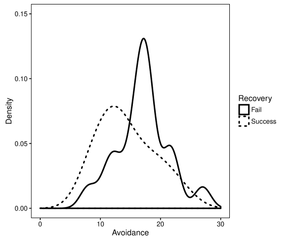
Figure 2: Smoothed densities of the distribution of cognitive avoidance for patients who managed to recover from cancer (Success) and for patients who did not recover (Fail) in the study of Epping-Jordan et al., (1994). Details are provided in Section 2.2.

In another study, Epping-Jordan et al., (1994) investigated the effect of cognitive avoidance on cancer recovery, by comparing the group of patients successfully recovering from cancer to those who failed to recover. The distribution of cognitive avoidance in both groups is displayed in Figure 2. While the distribution of patients not recovering is relatively symmetric, it is clearly right skewed for patients who did recover. Among others, the optimal design of $T_{U}$ for this special case is examined below. Again, the application of t-tests is questionable here and $T_{U}$ may be a sensible alternative. These examples show the relevance of the Wilcoxon-Mann-Whitney-test in biometrical applications. Thus, it is of interest to investigate its optimal design when distributions are known to be skewed and / or have unequal variances.

Using the normal approximation, the power of $T_{U}$ can be approximated as well. In the one-sided case, if the alternative hypothesis is $\operatorname{P}(X\geq Y)>0.5$ (equivalent to $a>0$ under $\operatorname{\mathcal{H}}_{1}$ (6) in case of continuous $X$ and $Y$), we have

$$\operatorname{Pow}_{N}(\omega)=1-\Phi\left(\frac{z_{1-\alpha}-\mu_{N}(\omega)}{\sigma_{N}(\omega)}\right).$$ (13)

In the two-sided case $\operatorname{P}(X\geq Y)\neq 0.5$ (equivalent to $a\neq 0$ under $\operatorname{\mathcal{H}}_{1}$ (6) in case of continuous $X$ and $Y$) we have

$$\operatorname{Pow}_{N}(\omega)=\Phi\left(\frac{z_{\alpha/2}-\mu_{N}(\omega)}{\sigma_{N}(\omega)}\right)-\Phi\left(\frac{z_{1-\alpha/2}-\mu_{N}(\omega)}{\sigma_{N}(\omega)}\right)+1.$$ (14)

Here, $\alpha$ denotes the nominal $\alpha$-level of the test, $\Phi$ the standard normal distribution function, and $z_{\alpha}$ the $\alpha$ quantile of the standard normal distribution. Unfortunately, finding the maximum of $\operatorname{Pow}_{N}$ in $\omega\in[0,1]$ analytically turns out to be unfeasible. For this reason, we present some examples for common distributions below and focus on the one-sided version of $T_{U}$, as the two-sided case yields nothing new concerning the optimal design despite a reduced power in general.

One of the most common cases of two-sample comparisons occurring for real data, which is not covered by Theorem 2, is the comparison of two normal distributions with unequal variances. The optimal design of $T_{U}$ was investigated for variance ratios ranging from $1/9$ to $9$ (or equivalently $1/3$ to $3$ in terms of standard deviation ratios), as the vast majority of real data comparisons can be expected to fall within this interval. Figure 3 (a) provides an overview on the applied normal densities. Recall that, in case of two normal samples with unequal variances, the optimal design of $T_{het}$ assigns a higher sample size to the sample with higher variance. Also, one may lose substantial power when variances are unequal but equally large samples are used (Dette and O’Brien,, 2004). Using the asymptotic power function (14), a different pattern can be found for $T_{U}$ (see Figure 4 (a) and (b) and (c)): When $F$ and $G$ are normal with $\sigma_{1}^{2}\neq\sigma_{2}^{2}$, the optimal design $\omega^{*}$, quite surprisingly, does not always favor the sample with the higher variance. Instead, the pattern appears to be more complex as displayed in Figure 4 (a). Furthermore, $\omega^{*}$ depends on the total sample size $N$ (see Figure 4 (b)) in a way that higher values of $N$ lead to slightly higher values of $\omega^{*}$ at least for the presented examples. Also, the optimal design depends very slightly on the $\alpha$-level (see Figure 4 (c)). To demonstrate that these findings are not just artifacts of the approximations, Figure 4 contains the simulated power based on 10,000 trials (dashed lines) along with the approximated power. From our perspective, the most important observation is that one generally loses only little power when choosing $\omega=0.5$ as compared to the optimal design $w^{*}$. To illustrate that this property may indeed not hold for $T_{het}$ when variances differ considerably (e.g., for a standard deviation ratio of $3$), its simulated power is also displayed in Figure 4 (a), (b), and (c) as grey lines.

Often enough, real data are not normally distributed, but skewed in some way as shown for the cancer studies of Sandler et al., (2003) and Epping-Jordan et al., (1994). Even though the central limit theorem ensures normally distributed means for $N\rightarrow\infty$ and thus the validity of the two-sample t-tests, sample sizes may be too small in many cases to ensure sufficient convergence to normality. Furthermore, even for larger (or infinitely large) samples, $T_{U}$ will be more efficient than the t-tests for many skewed distributions (Hodges and Lehmann,, 1956; Blair and Higgins,, 1980; Sawilowsky and Blair,, 1992). In fact, this can be considered one of the main reasons to apply the Wilcoxon-Mann-Whitney-test. Accordingly, the optimal design of $T_{U}$ for skewed distributions is of primary interest. In the absence of any general analytic solution for this case, we will again investigate the optimal design for selected examples. We chose to use exponential, log-normal and $\chi^{2}$-distributions to represent different shapes and amounts of skewness that are typically present in real data (e.g., for reaction or survival times). We decided to include only unimodal distributions, as multimodal distributions appear pretty rarely and usually indicate that different populations, each having a unimodal distributions, were mixed up (something that should be avoided to allow clear interpretation of scientific results). First, consider the canonical case of skewed distributions with the same shape but shifted mean, which, by definition, satisfy the stochastic ordering hypothesis (6). See Figure 3 (b) for a visualization of their densities. As can be seen from the power functions displayed in Figure 4 (d) and (e), $\omega^{*}$ varies with the degree of the shift, the total sample size, and (slightly) with the amount of skewness. Again however, $\omega=0.5$ is generally nearly as good as $w^{*}$. Leaving the stochastic ordering hypothesis, distributions with different amount of skewness were also compared to each other (densities are displayed in Figure 3 (c) and (d)). From the power functions in Figure 4 (f), (g), and (h), it is immediately evident that $\omega=0.5$ is again nearly optimal for all displayed comparisons.

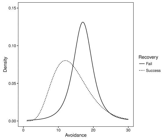
Figure 5: Approximated densities of the distribution of cognitive avoidance for patients who managed to recover from cancer (Success) and for patients who did not recover (Fail) in the study of Epping-Jordan et al., (1994). Details are provided in Section 2.2.

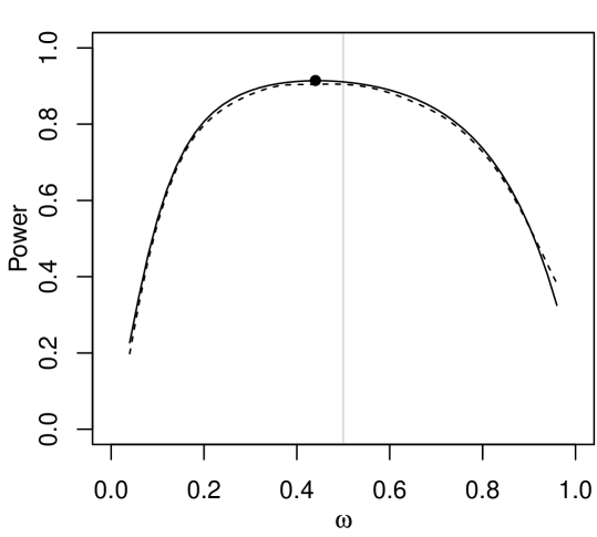
Figure 6: Power of $T_{U}$ applied to the study of Epping-Jordan et al., (1994). The vertical grey line indicates the position of the design $\omega=0.5$. Deficiency of $\omega=0.5$ relative to the optimal design: $1\%$. More details are provided in Section 2.2.

To end this section, we want to briefly and exemplary discuss the optimal design of $T_{U}$ for the cancer study of Epping-Jordan et al., (1994) mentioned above. Overall, $67$ patients participated in the study. The distribution of patients successfully recovering from cancer can be nicely approximated by a $\chi^{2}$ distribution with $14$ degrees of freedom, whereas the distribution of patients who failed to recover is similar to a Student-t distribution with $3$ degrees of freedom, location parameter of $17$, and scale parameter of $2.8$ (see Figure 5 for an illustration of the corresponding densities). When applying $T_{U}$ under these conditions to test whether the first group has smaller values than the second, we find the optimal design to be roughly $\omega^{*}\approx 0.45$ (see Figure 6) that is around $67\times 0.45\approx 30$ people should be assigned to the first group. Note that again, almost no power is lost when using equally large groups.

3 Conclusion

In the present paper, we demonstrated that assigning equally large sample sizes to both groups is generally a very good design for the Wilcoxon-Mann-Whitney-test. Using normal approximations, its optimality was proved for symmetric and identically shaped distributions. For a range of other distributions, we could show that $\omega=0.5$ offers power only negligibly lower than the optimal design that varies with the underlying distributions, the total sample size and the $\alpha$-level. Thus, in contrast to the t-tests for homogeneous and heterogeneous variances, equally large sample sizes can be used without the risk of substantially losing power. In this sense, the Wilcoxon-Mann-Whitney-test is not only valid and powerful for a wide range of distributions because of its non-parametric nature, but also offers a robust experimental design to be applied on.

The examples presented in the figures are only a subset of the cases we analyzed in order to come to our conclusions. However, since $F$ and $G$ come from an infinite space of distributions, there might still be relevant combinations, for which the design $\omega=0.5$ has considerably lower power than the optimal design, even for medium to large samples sizes. Ideally, we also wanted to provide a closed form of the optimal design for arbitrary $F$ and $G$. However, even when the (asymptotic) distribution under $\operatorname{\mathcal{H}}_{1}$ is known, it is practically unfeasible to solve for $\omega^{*}$ if $F$ and $G$ are not assumed to be symmetric and identically shaped. If one has a clear idea on how the data will be distributed and wants to get a more precise estimation of the optimal design (instead of just applying $\omega=0.5$), numerical optimization of the power function still appears to be the best option.

Appendix

A: Extension and proof of Lemma 1

Let $F$ and $G$ be some arbitrary (discrete or continuous) distributions with densities $f$ and $g$.

1. We have

   $$\operatorname{P}(X\geq Y)=\int{G(x)f(x)dx}.$$

2. The mean and the variance of $U_{mn}$ can be written as

   $$\operatorname{\mathbb{E}}(U_{mn}) =mn\operatorname{P}(X\geq Y),$$

   $$\operatorname{Var}(U_{mn}) =nm\bigg{(}\operatorname{P}(X\geq Y)-(n+m-1)\operatorname{P}(X\geq Y)^{2}$$

   $$\quad+(n-1)\int{G(x)^{2}f(x)dx}+(m-1)\int{(1-\tilde{F}(x))^{2}g(x)dx}\bigg{)}.$$

3. If $F$ and $G$ are symmetric with $G(x)=F(x+a)$ for fixed $a\in\mathbb{R}$ it holds that

   $$\int{G(x)^{2}f(x)dx}=\int{(1-\tilde{F}(x))^{2}g(x)dx}.$$

4. (supplemental) For continuous $F$ and $G$ under the null hypothesis $F=G$, it holds that

   $$\operatorname{\mathbb{E}}(U_{mn})=\operatorname{\mathbb{E}}_{0}(U_{mn})\text{ and }\operatorname{Var}(U_{mn})=\operatorname{Var}_{0}(U_{mn})$$

   that is the formulae above coincide with (5).

5. (supplemental) For continuous $F$ and $G$ we have

   $$\int{(1-F(x))^{2}g(x)dx}=\int{\left(\int_{-\infty}^{x}{G(y)f(y)dy}+G(x)(1-F(x))\right)f(x)dx}.$$

Proof.

$(i)$ and $(ii)$ See the Appendix of Lehmann and D’Abrera, (2006).

$(iii)$ Without loss of generality assume $\operatorname{\mathbb{E}}(X)=0$ so that $\operatorname{\mathbb{E}}(Y)=-a$ because $G(x)=F(x+a)$. Due to symmetry of $F$ and $G$ and since $G(x)=F(x+a)$, we have $f(x)=g(-a-x)$ and $G(x)=1-\tilde{F}(-a-x)$ for all $x\in\mathbb{R}$, which also means

$$f(x)G(x)^{2}=g(-a-x)(1-\tilde{F}(-a-x))^{2}.$$ (15)

In both integrals, integration is done over $\mathbb{R}$ so that the statement follows immediately.

$(iv)$ The statement is trivial for $\operatorname{\mathbb{E}}(U_{mn})$. For $F=G$ we have $\operatorname{P}(X\geq Y)=0.5$ and hence

$$\int{g(x)(1-F(x))^{2}dx}=1-2\operatorname{P}(X\geq Y)+\int{g(x)F(x)^{2}dx}=\int{f(x)G(x)^{2}dx}.$$ (16)

As per definition of the mean, we may write

$$\int{f(x)F(x)^{2}dx}=\operatorname{\mathbb{E}}(F(X)^{2}).$$ (17)

The distribution of the random variable $F(X)$ is known to be uniform in $[0,1]$, if $X$ has distribution $F$. Accordingly, it holds that

$$\operatorname{\mathbb{E}}(F(X)^{a})=\int_{0}^{1}{x^{a}dx}=\frac{1}{a+1}.$$ (18)

In particular for $F=G$, this means

$$\int{f(x)G(x)^{2}dx}=\int{g(x)(1-F(x))^{2}dx}=\frac{1}{3},$$ (19)

which directly leads to

$$\operatorname{Var}(U_{mn}) =mn\bigg{(}\frac{1}{2}+\frac{m+n-2}{3}-\frac{m+n-1}{4}\bigg{)}$$

$$=\frac{mn(6+4(m+n-2)-3(m+n-1))}{12}$$

$$=\frac{mn(m+n+1)}{12}.$$ (20)

Note that this statement does not hold when $F=G$ is discrete since $\operatorname{P}(X\geq Y)\neq 0.5$ in this case due to the presence of ties.
$(v)$ The proof relies on another derivation of a formula for $\operatorname{Var}(U_{mn})$: For $t\in\mathbb{N}$, $t\geq\max(m,n)$, we may write every sequence of $x_{1},...,x_{m}$, $y_{1},...,y_{n}$ ordered by size as

$$X_{1},Y_{1},X_{2},...,X_{t},Y_{t}$$ (21)

with $X_{i}\in\{0,...,m\}$ representing $X_{i}$ values out of $x_{i},...,x_{m}$ and $Y_{i}\in\{0,...,n\}$ representing $Y_{i}$ values out of $y_{i},...,y_{n}$. For instance, suppose that $t=m=n=3$ and that ordering the observations $x_{i},y_{i}$ ($1\leq i\leq 3$) have resulted in

$$x_{1},x_{2},y_{1},y_{2},x_{3},y_{3}.$$ (22)

Then, we could represent sequence (22) as

$$2(=X_{1}),2(=Y_{1}),1(=X_{2}),1(=Y_{2}),0(=X_{3}),0(=Y_{3}).$$ (23)

Note that $\sum_{i=1}^{t}{X_{i}}=m$ and $\sum_{i=1}^{t}{Y_{i}}=n$. We can now write $U_{mn}$ as

$$U_{mn}=\sum_{i=2}^{t}{\sum_{j=1}^{i-1}{X_{i}Y_{j}}}.$$ (24)

Assume that both $(X_{1},...,X_{t})$ and $(Y_{1},...,Y_{t})$ are multinomial distributed with probabilities $(f_{1},...,f_{t})$ and $(g_{1},...,g_{t})$ respectively. For every $X_{i}$, it holds that

$$\operatorname{\mathbb{E}}(X_{i})=mf_{i}\text{ and }\operatorname{\mathbb{E}}(X_{i}^{2})=mf_{i}(1-f_{i}+mf_{i}).$$ (25)

For $i\neq k$ we have

$$\operatorname{\mathbb{E}}(X_{i}X_{k})=m(m-1)f_{i}f_{k}.$$ (26)

The same goes, of course, for $Y_{i}$.

Defining $\widetilde{f}_{i,m}:=f_{i}(1-f_{i}-mf_{i})$ and $\widetilde{g}_{i,n}:=g_{i}(1-g_{i}-ng_{i})$, the second non-central moment $\operatorname{\mathbb{E}}(U_{mn}^{2})$ equals

$$\operatorname{\mathbb{E}}(U_{mn}^{2}) =\operatorname{\mathbb{E}}((\sum_{i=2}^{t}{\sum_{j=1}^{i-1}{X_{i}Y_{j}}})^{2})$$

$$=\sum_{i=2}^{t}{\sum_{j=1}^{j-1}{\operatorname{\mathbb{E}}(X_{i}^{2})\operatorname{\mathbb{E}}(Y_{j}^{2})}}+\sum_{i=3}^{t}{\sum_{j,l<i\atop j\neq l}{\operatorname{\mathbb{E}}(X_{i}^{2})\operatorname{\mathbb{E}}(Y_{j}Y_{l})}}$$

$$\quad+\sum_{i,k\leq t\atop i\neq k}{\sum_{j<i,k}{\operatorname{\mathbb{E}}(X_{i}X_{k})\operatorname{\mathbb{E}}(Y_{j}^{2})}}+\sum_{i,k\leq t\atop i\neq k}{\sum_{j<i;\text{ }l<k\atop j\neq l}{\operatorname{\mathbb{E}}(X_{i}X_{k})\operatorname{\mathbb{E}}(Y_{j}Y_{l})}}$$

$$=mn\bigg{(}\sum_{i=2}^{t}{\sum_{j=1}^{i-1}{\widetilde{f}_{i,m}\widetilde{g}_{j,n}}}+(n-1)\sum_{i=3}^{t}{\sum_{j,l<i\atop j\neq l}{\widetilde{f}_{i,m}g_{j}g_{l}}}$$

$$\quad+(m-1)\sum_{i,k\leq t\atop i\neq k}{\sum_{j<i,k}{f_{i}f_{k}\widetilde{g}_{j,n}}}+(m-1)(n-1)\sum_{i,k\leq t\atop i\neq k}{\sum_{j<i;\text{ }l<k\atop j\neq l}{f_{i}f_{k}g_{j}g_{l}}}\bigg{)}$$

$$=mn\bigg{(}\sum_{i=2}^{t}{\sum_{j=1}^{i-1}{\widetilde{f}_{i,m}\widetilde{g}_{j,n}}}+(n-1)(\sum_{i=3}^{t}{\widetilde{f}_{i,m}((\sum_{j<i}{g_{j}})^{2}-\sum_{j<i}{g_{j}^{2}})})$$

$$\quad+(m-1)(\sum_{i,k\leq t}{\sum_{j<i,k}{f_{i}f_{k}\widetilde{g}_{j,n}}}-\sum_{i\leq t}{\sum_{j<i}{f_{i}^{2}\widetilde{g}_{j,n}}})$$

$$\quad+(m-1)(n-1)(\sum_{i,k\leq t}{f_{i}f_{k}\sum_{j<i}{g_{j}}\sum_{l<k}{g_{l}}}-\sum_{i\leq t}{f_{i}^{2}(\sum_{j<i}{g_{j}})^{2}}-\sum_{i,k\leq t}{\sum_{j<i,k}{f_{i}f_{k}g_{j}^{2}}})\bigg{)}.$$ (27)

For non-empty finite sets $A_{t},B_{t}$ with $|A_{t}|=|B_{t}|=t$ define

$$f_{A_{t}}(x):=\Bigg{\{}\begin{array}[]{l}\frac{f(x)}{\sum_{x\in A_{t}}{f(x)}}\text{ if }x\in A_{t}\\ 0\qquad\qquad\text{else }\\ \end{array}\quad g_{B_{t}}(y):=\Bigg{\{}\begin{array}[]{l}\frac{g(y)}{\sum_{y\in B_{t}}{g(y)}}\text{ if }y\in B_{t}\\ 0\qquad\qquad\text{else.}\\ \end{array}$$ (28)

We choose $A_{t}$ and $B_{t}$ so that $x_{i}<y_{i}<x_{i+1}<y_{i+1}$ for all $x_{i}\in A_{t}$ and $y_{i}\in B_{t}$ as well as

$$\lim_{t\rightarrow\infty}\sum_{x_{i}\leq x}{f_{A_{t}}(x_{i})}=F(x)\qquad\lim_{t\rightarrow\infty}\sum_{y_{i}\leq y}{g_{B_{t}}(y_{i})}=G(y).$$ (29)

Since $F$ and $G$ are continuous, we have

$$\lim_{t\rightarrow\infty}f_{A_{t}}(x_{i})=\lim_{t\rightarrow\infty}g_{B_{t}}(y_{j})=0.$$ (30)

Together with $\sum_{i=1}^{t}{f_{A_{t}}(x_{i})}=\sum_{i=1}^{t}{g_{B_{t}}(y_{i})}=1$, it follows that

$$\lim_{t\rightarrow\infty}\sum_{i=1}^{t}{f_{A_{t}}(x_{i})^{2}}=\lim_{t\rightarrow\infty}\sum_{i=1}^{t}{g_{B_{t}}(y_{i})^{2}}=0.$$ (31)

Setting $f_{i}:=f_{A_{t}}(x_{i})$, $g_{i}:=g_{B_{t}}(y_{i})$ in (Proof.) and applying (31) leads to

$$\operatorname{\mathbb{E}}(U_{mn}^{2}) =mn\lim_{t\rightarrow\infty}\bigg{(}\sum_{i=2}^{t}{f_{A_{t}}(x_{i})\sum_{j<i}{g_{B_{t}}(y_{j})}}+(n-1)\sum_{i=3}^{t}{f_{A_{t}}(x_{i})(\sum_{j<i}{g_{B_{t}}(y_{j})})^{2}}$$

$$\quad+(m-1)\sum_{i,k\leq t}{f_{A_{t}}(x_{i})f_{A_{t}}(x_{k})\sum_{j<i,k}{{g_{B_{t}}(y_{j})}}}$$

$$\quad+(m-1)(n-1)(\sum_{i,k\leq t}{f_{A_{t}}(x_{i})f_{A_{t}}(x_{k})\sum_{j<i}{g_{B_{t}}(y_{j})}\sum_{l<k}{g_{B_{t}}(y_{l})}}\bigg{)}$$

$$=mn\lim_{t\rightarrow\infty}\bigg{(}\sum_{i=2}^{t}{f_{A_{t}}(x_{i})\sum_{j<i}{g_{B_{t}}(y_{j})}}+(n-1)\sum_{i=3}^{t}{f_{A_{t}}(x_{i})(\sum_{j<i}{g_{B_{t}}(y_{j})})^{2}}$$

$$\quad+(m-1)\sum_{i\leq t}{f_{A_{t}}(x_{i})\sum_{k\leq t}f_{A_{t}}(x_{k})\sum_{j<i,k}{{g_{B_{t}}(y_{j})}}}$$

$$\quad+(m-1)(n-1)\sum_{i\leq t}f_{A_{t}}(x_{i})\sum_{j<i}{g_{B_{t}}(y_{j})}\sum_{k\leq t}f_{A_{t}}(x_{k})\sum_{l<k}g_{B_{t}}(y_{l})\bigg{)}.$$ (32)

Going from sums to integrals and simplifying yields

$$\operatorname{\mathbb{E}}(U_{mn}^{2}) =mn\bigg{(}\int{f(x)G(x)dx}+(n-1)\int{f(x)G(x)^{2}dx}$$

$$\quad+(m-1)\int f(x)\int f(y)\,G(\min(x,y))dydx$$

$$\quad+(m-1)(n-1)\left(\int{f(x)G(x)dx}\right)^{2}\bigg{)}$$

$$=mn\bigg{(}\operatorname{P}(X\geq Y)+(n-1)\int{f(x)G(x)^{2}dx}$$

$$\quad+(m-1)\int f(x)\left(\int_{-\infty}^{x}f(y)G(y)dy+G(x)(1-F(x))\right)dx$$

$$\quad-(m+n-1)\operatorname{P}(X\geq Y)^{2}\bigg{)}+\operatorname{\mathbb{E}}(U_{mn})^{2}.$$ (33)

Since $\operatorname{Var}(U_{mn})=\operatorname{\mathbb{E}}(U_{mn}^{2})-\operatorname{\mathbb{E}}(U_{mn})^{2}$ the statement follows by comparing this variance formula to the formula in $(ii)$. ∎

Figure 1: Graph of the approximate deficiency of the Wilcoxon-Mann-Whitney-test for symmetric and identically shaped distributions.

(a) Normal densities corresponding to Subfigure (a), (b) and (c) in Figure 4.

(b) Shifted skewed densities corresponding to Subfigure (d) and (e) in Figure 4.

(c) Skewed densities corresponding to Subfigure (f) in Figure 4.

(d) Skewed densities corresponding to Subfigure (g) and (h) in Figure 4.

Figure 3: Densities of the distributions used for the power calculations displayed in Figure 4. The density of $G$ is plotted in bold. Abbreviations: $\mathcal{N}(\mu,\sigma)=$ Normal distribution with mean $\mu$ and standard deviation $\sigma$; $\chi^{2}(df)=$ Chi-square distribution with $df$ degrees of freedom; $LN(\mu,\sigma)=$ Log-normal distribution with log-mean $\mu$ and log-standard deviation $\sigma$; $Exp(\lambda)=$ Exponential distribution with rate $\lambda$.

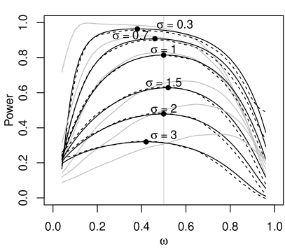
(a) Varied $\sigma$: $\mathcal{N}(0.75,\sigma)$ vs. $\mathcal{N}(0,1)$. $D_{U}(0.5)$: $0-4\%$; $D_{het}(0.5)$: $0-24\%$.

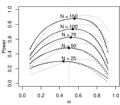
(b) Varied $N$: $\mathcal{N}(0.75,2)$ vs. $\mathcal{N}(0,1)$. $D_{U}(0.5)$: $0-2\%$; $D_{het}(0.5)$: $0-12\%$.

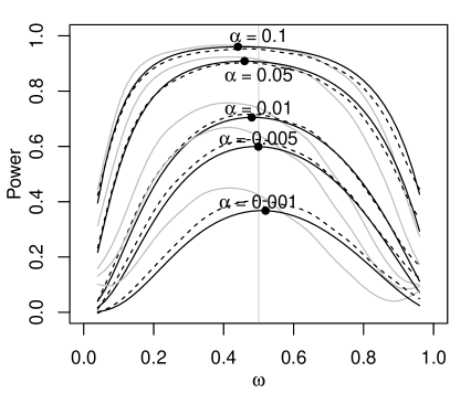
(c) Varied $\alpha$: $\mathcal{N}(0.75,0.7)$ vs. $\mathcal{N}(0,1)$. $D_{U}(0.5)$: $0-2\%$; $D_{het}(0.5)$: $0-10\%$.

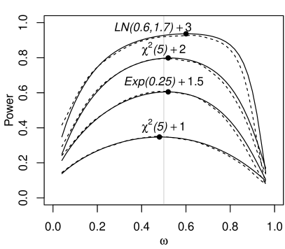
(d) Varied $F$ and $a$: $G(x)=F(x+a)$. $D_{U}(0.5)$: $0-2\%$.

(e) Varied $N$: $\chi^{2}(5)+1.5$ vs. $\chi^{2}(5)$. $D_{U}(0.5)$: $0-2\%$.

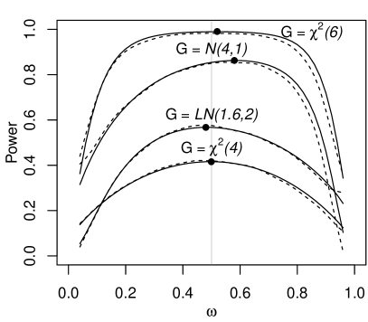
(f) Varied $F$: $G=\chi^{2}(3)$. $D_{U}(0.5)$: $0-2\%$.

(g) Varied $F$: $G=Exp(0.75)$. $D_{U}(0.5)$: $0-2\%$.

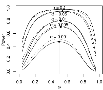
(h) Varied $\alpha$: $Exp(0.25)$ vs. $Exp(0.75)$. $D_{U}(0.5)$: $0-2\%$.

Figure 4: Power of $T_{U}$ for $N=50$ and $\alpha=0.05$ unless otherwise specified. Vertical grey lines indicate the position of the design $\omega=0.5$. $D_{U}(0.5)$ and $D_{het}(0.5)$ indicate the deficiency of $\omega=0.5$ relative to the optimal design for $T_{U}$ and $T_{het}$ respectively. Abbreviations: $\mathcal{N}(\mu,\sigma)=$ Normal distribution with mean $\mu$ and standard deviation $\sigma$; $\chi^{2}(df)=$ Chi-square distribution with $df$ degrees of freedom; $LN(\mu,\sigma)=$ Log-normal distribution with log-mean $\mu$ and log-standard deviation $\sigma$; $Exp(\lambda)=$ Exponential distribution with rate $\lambda$.

References

- Agresti, (2013) Agresti, A. (2013). Categorical data analysis. John Wiley & Sons.
- Arap et al., (1998) Arap, W., Pasqualini, R., and Ruoslahti, E. (1998). Cancer treatment by targeted drug delivery to tumor vasculature in a mouse model. Science, 279(5349):377–380.
- Atkinson et al., (2007) Atkinson, A. C., Donev, A. N., and Tobias, R. D. (2007). Optimum experimental designs, with SAS, volume 34. Oxford University Press Oxford.
- Berger and Wong, (2009) Berger, M. P. and Wong, W.-K. (2009). An introduction to optimal designs for social and biomedical research, volume 83. John Wiley & Sons.
- Blair and Higgins, (1980) Blair, R. C. and Higgins, J. J. (1980). A comparison of the power of Wilcoxon’s rank-sum statistic to that of Student’s t statistic under various nonnormal distributions. Journal of Educational and Behavioral Statistics, 5(4):309–335.
- Brunner and Munzel, (2002) Brunner, E. and Munzel, U. (2002). Nichtparametrische Datenanalyse, volume 34. Springer.
- Dette and Munk, (1997) Dette, H. and Munk, A. (1997). Optimum allocation of treatments for Welch’s test in equivalence assessment. Biometrics, 52(3):1143–1150.
- Dette and O’Brien, (2004) Dette, H. and O’Brien, T. E. (2004). Efficient experimental design for the Behrens-Fisher problem with application to bioassay. The American Statistician, 58(2):138–143.
- Di Bisceglie et al., (1989) Di Bisceglie, A. M., Martin, P., Kassianides, C., Lisker-Melman, M., Murray, L., Waggoner, J., Goodman, Z., Banks, S. M., and Hoofnagle, J. H. (1989). Recombinant interferon alfa therapy for chronic hepatitis c. New England Journal of Medicine, 321(22):1506–1510.
- Epping-Jordan et al., (1994) Epping-Jordan, J. E., Compas, B. E., and Howell, D. C. (1994). Predictors of cancer progression in young adult men and women: avoidance, intrusive thoughts, and psychological symptoms. Health Psychology, 13(6):539.
- Fay and Proschan, (2010) Fay, M. P. and Proschan, M. A. (2010). Wilcoxon-Mann-Whitney or t-test? On assumptions for hypothesis tests and multiple interpretations of decision rules. Statistics Surveys, 4:1–39.
- Hodges and Lehmann, (1956) Hodges, J. L. and Lehmann, E. L. (1956). The efficiency of some nonparametric competitors of the t-test. The Annals of Mathematical Statistics, 27(2):324–335.
- Hoeffding, (1948) Hoeffding, W. (1948). A class of statistics with asymptotically normal distribution. The Annals of Mathematical Statistics, 19(3):293–325.
- Hollander et al., (2013) Hollander, M., Wolfe, D. A., and Chicken, E. (2013). Nonparametric statistical methods. John Wiley & Sons.
- Holling and Schwabe, (2013) Holling, H. and Schwabe, R. (2013). An introduction to optimal design: Some basic issues using examples from dyscalculia research. Zeitschrift für Psychologie, 221(3):124–144.
- Lanquillon et al., (2000) Lanquillon, S., Krieg, J., Bening-Abu-Shach, U., and Vedder, H. (2000). Cytokine production and treatment response in major depressive disorder. Neuropsychopharmacology, 22(4):370–379.
- Lehmann, (1951) Lehmann, E. L. (1951). Consistency and unbiasedness of certain nonparametric tests. The Annals of Mathematical Statistics, 22(2):165–179.
- Lehmann and D’Abrera, (2006) Lehmann, E. L. and D’Abrera, H. J. (2006). Nonparametrics: statistical methods based on ranks. Springer New York.
- Lehmann and Romano, (2006) Lehmann, E. L. and Romano, J. P. (2006). Testing statistical hypotheses. Springer.
- Mann and Whitney, (1947) Mann, H. B. and Whitney, D. R. (1947). On a test of whether one of two random variables is stochastically larger than the other. The Annals of Mathematical Statistics, 18(2):50–60.
- Misiani et al., (1994) Misiani, R., Bellavita, P., Fenili, D., Vicari, O., Marchesi, D., Sironi, P. L., Zilio, P., Vernocchi, A., Massazza, M., Vendramin, G., et al. (1994). Interferon alfa-2a therapy in cryoglobulinemia associated with hepatitis c virus. New England Journal of Medicine, 330(11):751–756.
- Mood, (1954) Mood, A. M. (1954). On the asymptotic efficiency of certain nonparametric two-sample tests. The Annals of Mathematical Statistics, 25(3):514–522.
- Sandler et al., (2003) Sandler, R. S., Halabi, S., Baron, J. A., Budinger, S., Paskett, E., Keresztes, R., Petrelli, N., Pipas, J. M., Karp, D. D., Loprinzi, C. L., et al. (2003). A randomized trial of aspirin to prevent colorectal adenomas in patients with previous colorectal cancer. New England Journal of Medicine, 348(10):883–890.
- Sawilowsky and Blair, (1992) Sawilowsky, S. S. and Blair, R. C. (1992). A more realistic look at the robustness and type ii error properties of the t test to departures from population normality. Psychological Bulletin, 111(2):352.
- Shen et al., (2008) Shen, W., Flajolet, M., Greengard, P., and Surmeier, D. J. (2008). Dichotomous dopaminergic control of striatal synaptic plasticity. Science, 321(5890):848–851.
- Sprent and Smeeton, (2007) Sprent, P. and Smeeton, N. C. (2007). Applied nonparametric statistical methods. CRC Press.
- Van der Vaart, (1950) Van der Vaart, H. (1950). Some remarks on the power function of Wilcoxon’s test for the problem of two samples. In Nederl. Akad. Wetensch., Proc., Ser. A, pages 494–520.
- Welch, (1938) Welch, B. L. (1938). The significance of the difference between two means when the population variances are unequal. Biometrika, 29(3–4):350–362.
- Wilcoxon, (1945) Wilcoxon, F. (1945). Individual comparisons by ranking methods. Biometrics Bulletin, 1(6):80–83.