An Origin Story for Amplitudes

Abstract

We classify origin limits of maximally helicity violating multi-gluon scattering amplitudes in planar $\mathcal{N}=4$ super-Yang-Mills theory, where a large number of cross ratios approach zero, with the help of cluster algebras. By analyzing existing perturbative data, and bootstrapping new data, we provide evidence that the amplitudes become the exponential of a quadratic polynomial in the large logarithms. With additional input from the thermodynamic Bethe ansatz at strong coupling, we conjecture exact expressions for amplitudes with up to 8 gluons in all origin limits. Our expressions are governed by the tilted cusp anomalous dimension evaluated at various values of the tilt angle.

“Those who explore an unknown world are travelers without a map: the map is the result of the exploration. The position of their destination is not known to them, and the direct path that leads to it is not yet made.” - Hideki Yukawa

I Introduction

For generic kinematics, perturbative scattering amplitudes can be extremely complicated functions of the kinematic variables. In certain limits, they may simplify enormously. For general gauge theories, simplifying kinematics include Sudakov regions, where soft gluon radiation is suppressed, and high-energy or multi-Regge limits, where Regge factorization holds. In planar $\mathcal{N}=4$ super-Yang-Mills theory (SYM), the duality of amplitudes to polygonal Wilson loops [1, 2, 3, 4] allows near-collinear limits to be computed [5, 6] in terms of excitations of the Gubser-Klebanov-Polyakov flux tube [7, 8]. Recently, an even simpler kinematical region for six-gluon scattering in the maximally-helicity-violating (MHV) configuration was found [9, 10], the origin where all three cross ratios of the dual hexagon Wilson loop are sent to zero. In this limit, the logarithm of the MHV amplitude becomes quadratic in the logarithms of the cross ratios. The coefficients of the two quadratic polynomials, $\Gamma_{\rm oct}$ and $\Gamma_{\rm hex}$, can be computed for any value of the ’t Hooft coupling $\lambda\equiv g^{2}/(16\pi^{2})$ by deforming the Beisert-Eden-Staudacher (BES) kernel [11] by a tilt angle $\alpha$, giving rise to a “tilted cusp anomalous dimension” $\Gamma_{\alpha}(g)$ (see eq. (30)). The usual BES kernel and cusp anomalous dimension are recovered by setting $\alpha=\pi/4$, $\Gamma_{\rm cusp}=\Gamma_{\alpha=\pi/4}$, while the two hexagon-origin coefficients are given by $\Gamma_{\rm oct}=\Gamma_{\alpha=0}$ and $\Gamma_{\rm hex}=\Gamma_{\alpha=\pi/3}$.

This Letter will explore analogous origins for higher-point MHV amplitudes, regions where the same quadratic logarithmic (QL) behavior holds. We will see that there is a cornucopia of such regions at seven and especially eight points. The regions need not be isolated points; they can be one-dimensional lines starting at seven points, and up to three-dimensional surfaces starting at eight points. They can be classified by cluster algebras [12, 13], which provide natural compactifications of the space of positive kinematics [14, 15, 16, 17], at the boundary of which these limits are located. Furthermore, we will provide a master formula that we conjecture organizes the QL behavior of MHV amplitudes in all of these regions for arbitrary coupling, as a discrete sum over tilt angles, in which $\Gamma_{\alpha}(g)$ carries all of the coupling dependence. Our formula is motivated by studying the thermodynamic Bethe ansatz (TBA) representation [18, 19, 5, 20] of the minimal-area formula [1] for the amplitude at strong coupling.

II Classifying Origin Limits

Dual conformal symmetry [21, 1, 2, 3, 4] in planar $\mathcal{N}=4$ SYM implies that MHV amplitudes for $n$ gluons depend on $3(n-5)$ independent kinematical variables. These may be chosen as a subset of the $n(n-5)/2$ dual conformal cross ratios,

$$u_{i,j}=\frac{x_{i,j+1}^{2}x_{j,i+1}^{2}}{x_{i,j}^{2}x_{j+1,i+1}^{2}}\,,$$ (1)

where $x_{i,j}^{\mu}\equiv p_{i}^{\mu}+p_{i+1}^{\mu}+\cdots+p_{j-1}^{\mu}$ are sums of cyclicly adjacent gluon momenta, and indices are always mod $n$.

For $n=6$, all cross ratios $u_{i}\equiv u_{i+1,i+4}$, $i=1,2,3$ are independent, and the origin limit is simply defined as the kinematic point

$$\text{O}^{(6)}:\ \ u_{i}\to 0\,,\quad i=1,2,3.$$ (2)

At higher $n$, there are $(n-5)(n-6)/2$ Gram determinant polynomial relations between the cross ratios, because there are a limited number of independent vectors in fixed spacetime dimensions. (For their explicit form for $n=7,8$, see appendix B.) These relations raise the question of how to define the appropriate generalizations of the origin limit.

To answer this question, we consider the positive region, a subregion of Euclidean scattering kinematics where amplitudes are expected to be devoid of branch points [15, 22]. Thus the first place to look for simple divergent behavior is at pointlike limits at the boundary of the positive region. Such limits may be found systematically using cluster algebras [12, 13] associated with the Grassmannian ${\rm Gr}(4,n)$ [23], which provide a compactification of the positive region [14, 15, 16, 17], see also [24]. Accordingly, the positive region may be mapped to the inside of a polytope, whose boundary comprises vertices connected by edges that bound polygonal faces, that bound higher-dimensional polyhedra. Cluster algebras, or more precisely cluster Poisson varieties, consist of a collection of clusters, each containing $3(n-5)$ cluster $\mathcal{X}$-coordinates $\mathcal{X}_{i}$, corresponding to a coordinate chart describing this compactification. Setting all $\mathcal{X}_{i}\to 0$ yields a vertex at the boundary of the positive region. Letting all but one $\mathcal{X}_{i}$ vanish gives an edge connecting neighboring clusters, known as a mutation. It is also associated with a birational transformation between the $\mathcal{X}$-coordinates of the connected clusters, enabling the generation of a cluster algebra from an initial cluster.

Origin Class	$u_{1}$	$u_{2}$	$u_{3}$	$u_{4}$	$u_{5}$	$u_{6}$	$u_{7}$	$u_{8}$	$v_{1}$	$v_{2}$	$v_{3}$	$v_{4}$
$\text{O}_{1}(\textrm{super})$	0	0	0	0	0	0	0	0	0	1	0	1
$\text{O}_{2}$	0	0	0	0	0	0	0	1	0	1	0	1
$\text{O}_{3}$	0	0	0	0	0	0	0	1	0	0	1	1
$\text{O}_{4}$	0	0	0	0	0	0	1	1	0	0	1	0
$\text{O}_{5}$	0	0	0	0	0	1	0	1	0	0	1	0
$\text{O}_{6}$	0	0	0	0	1	0	0	1	0	1	0	0
$\text{O}_{7}$	0	0	0	0	1	0	0	1	0	0	1	0
$\text{O}_{8}$	0	0	0	1	0	0	0	1	0	1	0	0
$\text{O}_{9}$	0	0	0	1	0	0	0	1	0	0	0	1

Table 1: All dihedrally inequivalent origin classes for $n=8$. Zeros represent infinitesimal values. There are nine infinitesimal cross ratios for all origins except for the super-origin $\text{O}_{1}$ which has ten. All nonzero cross ratios are close to unity.

We start with the finite ${\rm Gr}(4,n)$ cluster algebras for $n=6,7$, with Dynkin labels $A_{3}$ and $E_{6}$ [13]. We first observe that in all boundary vertices, $u_{i,j}=0$ or $1$. These kinematic points contain the $n=6$ origin limit (2); at $n=7$ we find 28 clusters describing analogous limits where all but one of the seven $u_{i}\equiv u_{i+1,i+4}$, $i=1,2,\ldots,7$, vanishes,

$$\text{O}_{j}^{(7)}:\ u_{i\neq j}\to 0\,,\quad u_{j}=1\,.$$ (3)

The seven origins are related by a cyclic symmetry, $u_{i}\mapsto u_{i+1}$. There are four clusters for each $\text{O}_{j}^{(7)}$, two with a different direction of approach to the limit, plus their parity images. All of these clusters form a cyclic chain connected by mutations or lines in the space of kinematics. In terms of cross ratios, the line connecting $\text{O}_{7}^{(7)}$ and $\text{O}_{1}^{(7)}$ is

$$\hbox{\sc Line 71}:\ \ u_{i}\ll 1,\quad i=2,3,4,5,6;\quad u_{7}+u_{1}=1\,,$$ (4)

with $u_{1},u_{7}\in[0,1]$. The remaining lines are obtained by cyclic symmetry. Quite remarkably, the amplitude exhibits exponentiated QL behavior not only on the points (3), but also on these origin lines! This QL behavior also implies that the value of the amplitude is independent of the direction or speed of approach to the limit; it remains the same function of the cross ratios irrespective of the rate with which they tend to zero.

Inspired by these examples, we define origin points at higher $n$ as vertices where at least $3(n-5)$ cross ratios approach zero. We now classify the $n=8$ origin points. While the corresponding ${\rm Gr}(4,8)$ cluster algebra is infinite-dimensional, there is a procedure for selecting a finite subset of clusters [25, 26, 22, 27, 28] based on tropicalization [29], see also [30]. Here we start with a cluster corresponding to an origin point, and generate new clusters by mutations until this condition is no longer met. We find 1188 clusters contained in the finite subset selected in [25, 26, 22, 27, 28], as further described in appendix C and in an ancillary file. Modding out by parity, dihedral symmetry and direction of approach, these origins belong to the nine classes shown in table 1, where $u_{i}\equiv u_{i+1,i+4}$, $i=1,2,\ldots,8$, and $v_{i}\equiv u_{i+1,i+5}$, $i=1,2,3,4$. This table may be obtained even more simply by assuming that all cross ratios approach 0 or 1, and scanning for all combinations that satisfy the Gram determinant constraints. This process also identifies one more potential origin, $\text{O}_{\rm X}=(0,0,1,0,0,1,0,1;0,0,0,0)$ in the $(u_{i};v_{j})$ notation of table 1. It lies outside of the positive region, and we defer its study to future work.

Figure 1: The system of eight-point origins exhibiting QL behavior. We omit many origins that are related to the ones shown by dihedral symmetry. The node numbers correspond to $\text{O}_{i}$ in table 1 or their dihedral images. The behavior on the lines and surfaces shown in the figure is also QL, except for the dashed line between $\text{O}_{1}$ and $\text{O}_{2}$.

At $n=8$, there are also higher-dimensional QL surfaces connecting the $\text{O}_{i}$, which generalize the seven-point Line 71 (4). Motivated by this line, which also defines an $A_{1}$ subalgebra of the $E_{6}$ cluster algebra, we searched for maximal subalgebras of the ${\rm Gr}(4,8)$ cluster algebra that move one solely from origin to origin. Two $A_{3}$ subalgebras correspond to two cubes, Cube 6789 and Cube 5678 . Two $A_{2}$ subalgebras correspond to Pentagon 345 and Pentagon 234. An $A_{1}\times A_{1}$ corresponds to Square 456. An $A_{1}$ subalgebra Superline 1 connects two super-origins $\text{O}_{1}$. These high-dimensional spaces interpolating between origins are summarized in table 2 and are depicted in figure 1.

Boundary	Relations
Cube 6789	$u_{3}+u_{4}=u_{7}+u_{8}=v_{1}+v_{4}=1$
Cube 5678	$u_{1}+u_{2}=u_{4}+u_{5}=v_{2}+v_{3}=1$
Square 456	$u_{1}+u_{2}=u_{7}+u_{8}=v_{4}=1$
Pentagon 345	$u_{8}+u_{1}u_{7}=u_{7}+u_{8}v_{4}=v_{4}+u_{7}v_{3}=1$
Pentagon 234	$u_{1}+u_{8}v_{3}=v_{3}+u_{1}v_{4}=u_{8}+u_{1}v_{1}=1$
Superline 1	$v_{1}=1-v_{2}=v_{3}=1-v_{4}$

Table 2: Relations among the finite cross ratios for the octagon boundaries. All the cross ratios unspecified in the relations are implicitly infinitesimal.

III Perturbative Data & Bootstrap

In this Letter we work with the $n$-point remainder function $R_{n}$, related to the MHV amplitude by

$$\exp R_{n}\equiv{A_{n}^{\text{MHV}}}/{A_{n}^{\text{BDS}}}\,,$$ (5)

where the known, infrared-divergent normalization factor $A_{n}^{\text{BDS}}$ is essentially the exponential of the one-loop amplitude [32, 33, 34]. The remainder function is infrared finite, and invariant under dual conformal symmetry as well as the $n$-gon dihedral symmetry group $D_{n}$.

Using perturbative data through seven loops, $R_{6}$ was found to simplify drastically [9] at the origin (2): To $\mathcal{O}(u_{i}^{0})$, it becomes the sum of two QL polynomials,

$$R_{6}{=-\tfrac{\Gamma_{0}-\Gamma_{\pi/4}}{24}\ln^{2}{(u_{1}u_{2}u_{3})}-\tfrac{\Gamma_{\pi/3}-\Gamma_{\pi/4}}{24}\sum_{i=1}^{3}\ln^{2}{(\tfrac{u_{i}}{u_{i+1}})}}\,,$$ (6)

where each polynomial is multiplied by the tilted cusp anomalous dimension $\Gamma_{\alpha}$ evaluated at different angles $\alpha=0,\tfrac{\pi}{4},\tfrac{\pi}{3}$ [10]. For $n=6$, $D_{6}$ acts on the $u_{i}$ as arbitrary $S_{3}$ permutations. The origin preserves this symmetry, so only $S_{3}$-symmetric quadratic polynomials are allowed, which are exhausted by those of eq. (6).

For $n=7$, QL behavior was observed for $R_{7}$ through four loops at the dihedrally-equivalent origins $\text{O}_{j}^{(7)}$ [35]. More generally, a four-loop computation along the lines of ref. [35] reveals that the remainder function $R_{7}$ on Line 71 (4) is given by,

$$R_{7}({\hbox{\sc Line 71}})=\sum_{i=1}^{3}c_{i}P_{i}^{(7)}\,,$$ (7)

where

$$P_{1}^{(7)} =\sum_{i=1}^{6}l_{i}l_{i+1}+\sum_{i=1}^{5}l_{i}l_{i+2}\,,$$

$$P_{2}^{(7)} =-l_{1}l_{7}+\sum_{i=1}^{7}l_{i}^{2}+\sum_{i=1}^{4}l_{i}l_{i+3}\,,$$

$$P_{3}^{(7)} =\sum_{i=1}^{7}l_{i}l_{i+2}-\sum_{i=1}^{3}l_{i}l_{i+4}\,,$$ (8)

are quadratic polynomials in the logarithms, $l_{i}\equiv\ln u_{i}$. In eq. (7) and in the following, we give only the leading QL behavior in the given limit. We never find any linear-logarithmic terms. There are constant terms followed by subleading power corrections, which we do not study.

Through four loops, the coefficients $c_{i}$ in eq. (7) are given by,

$$c_{1} =g^{4}\zeta_{2}-\tfrac{37}{2}g^{6}\zeta_{4}+g^{8}\left(\tfrac{1975}{8}\zeta_{6}-2\zeta_{3}^{2}\right)+O(g^{10})\,,$$

$$c_{2} =-\tfrac{5}{2}g^{6}\zeta_{4}+g^{8}\left(\tfrac{413}{8}\zeta_{6}-2\zeta_{3}^{2}\right)+O(g^{10})\,,$$ (9)

$$c_{3} =-\tfrac{35}{8}g^{8}\zeta_{6}+O(g^{10})\,,$$

where $\zeta_{n}=\sum_{k=1}^{\infty}k^{-n}$ is the Riemann zeta value.

We can derive the decomposition (7) to all loop orders via a “baby” amplitude boostrap, using the following conditions:

1. We assume that $R_{7}$ is QL.

2. Continuity: The result at $\text{O}^{(7)}_{7}$ ($\text{O}^{(7)}_{1}$) is obtained from that on Line 71 by setting $l_{7}\to 0$ ($l_{1}\to 0$).

3. Three conditions from dihedral symmetry:

   • The full $D_{7}$ is broken on the line but a single reflection (flip) survives: $u_{i}\leftrightarrow u_{8-i}$. It exchanges the two end points $u_{7}=1$ and $u_{1}=1$.

   • There is a flip symmetry at $u_{7}=1$: $u_{i}\leftrightarrow u_{7-i}$.

   • The behaviors at the two endpoints are related by cycling $u_{i}\mapsto u_{i+1}$.

4. The final-entry (FE) condition.

MHV amplitudes obey a FE condition, which controls their first derivatives [36]. For $n=6$ and general kinematics, the FE condition removes three of the nine symbol letters [37], namely $1-u_{i}$; but at the origin these letters are irrelevant because they approach $1$. Hence the six-point FE condition trivializes at the origin.

In contrast, the seven-point FE condition allows 14 symbol letters for general kinematics [38], which collapse on Line 71 to six letters out of a total of seven. We obtain a single constraint,

$$\bigl{[}u_{7}\partial_{u_{7}}+u_{1}\partial_{u_{1}}-u_{4}\partial_{u_{4}}\bigr{]}R_{7}=0\,,$$ (10)

where derivatives for $\ln u_{7}$ are taken independently of $\ln u_{1}$, despite the constraint $u_{7}+u_{1}=1$ on Line 71. Combining all constraints, the only allowed QL polynomials are exactly the three given in (III), and no linear-logarithmic structures survive. That is, the possible kinematic dependence of $R_{7}$ is already saturated by (III) at four loops. We will see that the TBA at strong coupling leads to precisely the same three $P_{i}^{(7)}$, and to a natural conjecture for all higher-loop corrections to the coefficients, which matches (III) through four loops.

The symbol of the eight-point remainder function $R_{8}$ is known at two and three loops [39, 40]; it vanishes at all the origins and interpolating surfaces, as it must to be QL. For all the kinematics in table 2, we computed the full functions at two loops  and, in some cases, up to five loops using the pentagon operator product expansion (OPE) [6]. In all cases, we found that the remainder function $R_{8}$ is QL .

Furthermore, we repeated the all-loop seven-point analysis at eight points, starting on Cube 6789, and then going on to other adjacent regions, using continuity at the boundaries between regions, see figure 1. In all cases, we found precisely five independent QL polynomials obeying the restrictions. On Cube 6789, see table 2, they have the form,

$$R_{8}({\hbox{\sc Cube 6789}})=\sum_{i=1}^{5}d_{i}P_{i}^{({\sc C})}\,,$$ (11)

where,

$$P_{1}^{({\sc C})} =\sum_{i=1}^{8}l_{i}^{2}-2\sum_{i=1}^{4}l_{i}l_{i+4}-2(l_{3}-l_{7})(l_{4}-l_{8})\,,$$ (12)

$$P_{2}^{({\sc C})} =2\sum_{i=1}^{4}l_{i}l_{i+4}+(l_{3}-l_{7})(l_{4}-l_{8})+(l_{1}+l_{5})(\ell_{1}+\ell_{4})$$

$$+(l_{3}+l_{4}+l_{7}+l_{8})\ell_{3}+(l_{2}+l_{6})\ell_{2}+\sum_{i=1}^{4}\ell_{i}^{2}\,,$$ (13)

with $l_{i}\equiv\ln u_{i}$ and $\ell_{i}\equiv\ln v_{i}$. The lengthier $P^{({\sc C})}_{3,4,5}$ are provided in appendix D. One has $d_{3}=d_{4}=\zeta_{2}g^{4}$ through two loops; the remaining coefficients start at higher orders. The same form (11) applies in the other QL-connected regions, with the same $d_{i}$’s but different polynomials. Similarly, the baby bootstrap yields a five-polynomial ansatz for Superline 1; since it is disconnected from the other regions, it comes with its own set of coefficients, $f_{i}$. We give the expressions for all five polynomials in all possible regions, along with weak coupling expansions of the $d_{i}$ and $f_{i}$ coefficients through eight loops, in the ancillary files octagon_QL_formula.txt and octagon_QL_coefs.txt.

IV Master formula from TBA

Additional insight into the QL behavior of the amplitudes may be found at strong coupling using the AdS/CFT-dual string theory description, which maps the problem to computing the minimal world-sheet area for a string anchored on a null polygonal contour at the boundary of AdS [1]. Using the integrability of the classical string theory [43], it boils down to solving a set of non-linear TBA integral equations [18, 19]. We will now outline how the TBA equations can be linearized near origins. A (weighted) Fourier transformation from the TBA spectral parameter $\theta$ to a variable $z$, related to the tilt angle, converts the integral equations to a simple matrix equation, and allows us to express the minimal area (the logarithm of the strong-coupling amplitude) as a single integral over $z$. The crux of our finite-coupling conjecture is to move the ’t Hooft coupling $\sqrt{\lambda}$ inside the integral and absorb it into the tilted cusp anomalous dimension. The resulting master formula (21) can be evaluated either at finite coupling, or at weak coupling where it agrees with all the perturbative data reviewed above.

For the TBA analysis, we use coordinates $\{\sigma_{s},\tau_{s},\varphi_{s}\}$, $s=1,\ldots,n-5$, originally developed for analyzing the OPE [5, 6]. The TBA equations are for a family of $3(n-5)$ functions $Y_{a,s}(\theta)$, with $a=\{0,\pm 1\}$ [5, 20]:

$$\ln{Y}_{a,s}(\theta)=I_{a,s}(\theta)$$ (14)

$$\,\,\,+\sum_{b,t}\int\limits\frac{k_{a}(\theta)d\theta^{\prime}}{2\pi k_{b}(\theta^{\prime})}K_{a,s}^{b,t}(\theta-\theta^{\prime})\ln{(1+Y_{b,t}(\theta^{\prime}))}\,,$$

where the sum runs over $b=0,\pm 1$, $t=s,s\pm 1$, with $k_{a}(\theta)=i^{a}\sinh{(2\theta-i\pi a/2)}$ and for some kernels $K$. The driving terms $I_{a,s}$ encode the cross ratios, and are given explicitly in terms of the OPE coordinates,

$$I_{a,s}(\theta)=a\varphi_{s}-m_{a}\tau_{s}\cosh{\theta}+(-1)^{s}im_{a}\sigma_{s}\sinh{\theta}\,,$$ (15)

with $m_{a}=2\cos{(a\pi/4)}$. The dependence on the hyperbolic angle $\theta$ corresponds to a collection of interacting relativistic particles, of mass $m_{a}$ and charge $a$, coupled to various temperatures $1/\tau_{s}$ and chemical potentials $\varphi_{s}$.

Drawing inspiration from the hexagon ($n=6$) analysis [10, 44], we expect origins to map to extreme limits where the particles are subject to large chemical potentials, $|\varphi_{s}|\rightarrow\infty$, and to small temperatures, $\tau_{s}\rightarrow\infty$. There are several ways of taking limits for $n>6$. We may send each $\varphi_{s}$ to either $+\infty$ or $-\infty$, with each case labelled by a sequence $\Sigma_{n}=(h_{1},\ldots,h_{n-5})$ with $h_{s}=\varphi_{s}/|\varphi_{s}|$. In such limits, we expect the particles with $a=h_{s}$ to condense, and the remaining ones to decouple. Namely, for a given choice $\Sigma_{n}$, we assume that $Y_{a,s}(\theta)\gg 1$ if $a=h_{s}$ and $Y_{a,s}=0$ otherwise, and linearize eq. (14) using $\ln{(1+Y_{b,t})}\rightarrow\delta_{b,h_{t}}\ln{Y_{h_{t},t}}$. We also assume that the above conditions hold over the entire real $\theta$ axis.

The problem may then be solved by going to Fourier space. One defines

$$\hat{f}(z)=\int\limits_{-\infty}^{\infty}\frac{d\theta}{2\pi\cosh{(2\theta)}}z^{2i\theta/\pi}f(\theta)\,,$$ (16)

with a measure introduced to eliminate the weight in eq. (14) and with the Fourier variable $(2\ln{z})/\pi$, with $z>0$, introduced to rationalize all expressions. Setting $Y_{s}=Y_{h_{s},s},I_{s}=I_{h_{s},s}$, eq. (14) yields

$$\widehat{\ln{Y}_{s}}(z)=\sum_{t=1}^{n-5}\left[1-K_{n}(z)\right]^{-1}_{s,t}\,\hat{I}_{t}(z)\,,$$ (17)

with the square matrix $(K_{n}(z))_{s,t}=\int\frac{d\theta}{2\pi}K_{h_{s},s}^{h_{t},t}(\theta)z^{2i\theta/\pi}$. At strong coupling, $\sqrt{\lambda}=4\pi g\gg 1$, the remainder function is given by the TBA free energy [18, 19, 5], which becomes

$$R_{n}^{\textrm{string}} = -\frac{\sqrt{\lambda}}{\pi^{2}}\int_{0}^{\infty}\frac{dz}{z}\mathcal{S}_{n}(z)+\dots\,,$$ (18)

$$\mathcal{S}_{n}(z) \equiv \sum_{s=1}^{n-5}\widehat{I}_{s}(1/z)\widehat{\ln{Y}_{s}}(z)\,.$$ (19)

The ellipses stand for a simple term $\propto\Gamma_{\textrm{cusp}}$, to which we shall return shortly. Importantly, the integrand $\mathcal{S}_{n}(z)$ is a rational function of $z$. For any limit $\Sigma_{n}$, it may be cast into the form (see appendix E for details)

$$\mathcal{S}_{n}(z)=\frac{z(1-z^{3})\mathcal{P}^{\Sigma}_{n}(z)}{(1+z)(1+z^{2})(1-z^{3(n-4)})}\,,$$ (20)

where $\mathcal{P}^{\Sigma}_{n}(z)=z^{3n-14}\mathcal{P}^{\Sigma}_{n}(1/z)$ is a polynomial of degree $3n-14$ in $z$ and is quadratic in $\{\sigma_{s},\tau_{s},\varphi_{s}\}_{s=1,\ldots,n-5}$.

Eq. (18) may be turned into an all-order conjecture by bringing $\sqrt{\lambda}$ under the integral sign and promoting it to a full function of the variable $z$. To be precise, we conjecture that $R_{n}$ takes at finite coupling the form of a contour integral in the dual variable $z$,

$$R_{n}=-\frac{1}{2}\oint_{C_{n}}\frac{dz}{2\pi iz}(z-1/z)\tilde{\mathcal{G}}(z,g)\mathcal{S}_{n}(z)\,,$$ (21)

with $\tilde{\mathcal{G}}(z,g)=\mathcal{G}(z,g)-\Gamma_{\textrm{cusp}}(g)$ and with $\mathcal{G}(z,g)$ the tilted cusp anomalous dimension, viewed here as a function of $z=-e^{2i\alpha}$,

$$\mathcal{G}(z,g)=\Gamma_{\alpha}(g)\,.$$ (22)

Eq. (21) neatly factorizes the coupling dependence, which resides in $\mathcal{G}(z,g)$, and the kinematics, which sits in the string integrand $\mathcal{S}_{n}(z)$. The contour $C_{n}$ is a sum of small circles around the singularities of $\mathcal{S}_{n}(z)$; from eq. (20) they are poles on the unit circle $|z|=1$, mapping to real angles $\alpha$. The original string formula is recovered by using the strong coupling behavior [10]

$$\Gamma_{\alpha}\approx\frac{2\alpha\sqrt{\lambda}}{\pi^{2}\sin{(2\alpha)}}\,\,\,\,\Rightarrow\,\,\,\,\mathcal{G}(z)\approx-\frac{2\sqrt{\lambda}\log{(-z)}}{\pi^{2}(z-1/z)}\,.$$ (23)

The integral in eq. (18) follows from the term $\propto\mathcal{G}(z)$, by wrapping the contour on the logarithmic cut along $z>0$, whereas the term $\propto\Gamma_{\textrm{cusp}}=\Gamma_{\pi/4}$ accounts for the ellipses in eq. (18).

At finite coupling, one may calculate eq. (21) by residues, around the poles in eq. (20), and write

$$R_{n}=\sum_{\alpha}\tilde{\Gamma}_{\alpha}(g)\times P^{\Sigma_{n}}_{\alpha}(\{\sigma_{s},\tau_{s},\varphi_{s}\})\,,$$ (24)

with $\tilde{\Gamma}_{\alpha}=\Gamma_{\alpha}-\Gamma_{\textrm{cusp}}$ and with the sum running over

$$\alpha=\frac{\pi}{2}-\frac{\pi p}{3}-\frac{\pi k}{3(n-4)}\,,$$ (25)

with $k=1,\ldots,n-5$ and $p=0,1,2$. The associated polynomials $P^{\Sigma_{n}}_{\alpha}$ follow straightforwardly from the TBA analysis, but are too bulky to be shown here (see eq. (55)). At last, one may eliminate the OPE parameters in favor of the cross ratios, using general formulae in ref. [45]. In the limit $|\varphi_{s}|\gg\tau_{s}\gg 1$, with $\sigma_{s}$ held fixed, these relations reduce to simple mappings between the OPE parameters and the logarithms of the cross ratios.

For illustration, when $n=6$, one finds

$$u_{1}\approx e^{\tau+\sigma-|\varphi|}\,,\qquad u_{2}\approx e^{-2\tau}\,,\qquad u_{3}\approx e^{\tau-\sigma-|\varphi|}\,,$$ (26)

and eq. (24) and $P^{\Sigma_{6}}_{\alpha}$ give

$$R_{6}=-\sum_{\alpha=0,\pm\pi/3}\frac{\tilde{\Gamma}_{\alpha}(g)}{24}|l_{1}+e^{2i\alpha}l_{2}+e^{4i\alpha}l_{3}|^{2}\,,$$ (27)

in perfect agreement with ref. [10], using $\tilde{\Gamma}_{-\alpha}=\tilde{\Gamma}_{\alpha}$. For $n=7$, one gets

$$u_{1}\approx e^{\tau_{2}-\sigma_{2}-|\varphi_{2}|}\,, u_{2}\approx e^{-2\tau_{2}}\,, u_{3}u_{7}\approx e^{\tau_{2}+\sigma_{2}-|\varphi_{2}|}\,,$$ (28)

$$u_{6}\approx e^{\tau_{1}-\sigma_{1}-|\varphi_{1}|}\,, u_{5}\approx e^{-2\tau_{1}}\,, u_{4}u_{7}\approx e^{\tau_{1}+\sigma_{1}-|\varphi_{1}|}\,,$$

with $u_{7}=1$ for $\Sigma_{7}=(+,+)$, and $u_{3}+u_{4}=1$ for $\Sigma_{7}=(+,-)$, corresponding, respectively, to the origin $\text{O}_{7}^{(7)}$ and a cyclic image of Line 71. Using $P^{\Sigma_{7}}_{\alpha}$, we find a perfect agreement with the general decomposition for the heptagon line, eq. (7), with $c_{3}=a_{3}-a_{1}/2,c_{2}=-a_{3},c_{1}=a_{2}-a_{1}/2$, where

$$a_{j}=\frac{(-1)^{j}}{3\sqrt{3}}\sum_{k=1}^{3}(-1)^{k}\sin{(2\alpha_{k})}\cos{(2(j-1)\alpha_{k})}\tilde{\Gamma}_{\alpha_{k}}(g)\,,$$ (29)

and $\alpha_{1,2,3}=\{\pi/18,5\pi/18,7\pi/18\}$. The coefficients agree with the perturbative results (III), taking into account the weak-coupling expansion of the tilted cusp anomalous dimension [10], $\Gamma_{\alpha}(g)=4g^{2}-16\zeta_{2}g^{4}\cos^{2}{\alpha}+O(g^{6})$, as discussed further in appendix A.

One may proceed similarly for $n=8$ using $\Sigma_{8}=(+,+,+),(+,+,-),(+,-,+)$ and find three domains describing, respectively, the origin ${\rm O}_{9}$, a line ${\rm O_{3}}$–${\rm O_{4}}$, and a square ending on ${\rm O_{8},O_{9}}$ and two images of ${\rm O_{7}}$. In all of these cases, we found perfect agreement with the perturbative results, with the coefficients matching the two-loop predictions and the five-loop OPE results.

This analysis does not exhaust all the origins and domains given in table 2. For example, for (an image of) Cube 6789 it covers but a single face. To reach the missing domains, one should look at a broader class of scalings, where not only $\varphi_{s}$ and $\tau_{s}$ are allowed to be large but also $\sigma_{s}$. These scalings are harder to address in general, because the limit $|\sigma_{s}|\rightarrow\infty$ generates large fluctuations in the $Y$ functions, making it hard to decide which of them are large and which are small. It may also trigger new exceptional solutions, with more particle species condensing simultaneously. In appendix F, we argue that this happens at $n=8$ for Superline 1; we conjecture that its QL behavior is captured by a system of linearized TBA equations based on 4 large $Y$ functions.

V Conclusions

In this letter we initiated a systematic exploration of origins: kinematical points and interpolating higher-dimensional surfaces where high-multiplicity MHV scattering amplitudes in planar $\mathcal{N}=4$ SYM simplify dramatically and can be predicted (conjecturally) at finite coupling. Cluster algebras provide a roadmap to the kinematics, while the TBA and the tilted cusp anomalous dimension $\Gamma_{\alpha}(g)$ both play a central role in the master formula for the leading singular behavior. We expect further kinematical richness to emerge for $n>8$, based on the appearance of the super-origin $\text{O}_{1}$ at $n=8$, which is not connected (by any QL lines) to the other eight-point origins. We also have not ruled out the possibilities of even more kinematic boundaries of the positive region with QL behavior, especially for $n\geq 8$. The behavior in all these regions will certainly play a key role in constraining the all-orders behavior of MHV amplitudes for generic kinematics. Our findings may also have implications for other planar ${\cal N}=4$ observables, such as correlators of large-charge operators, which exhibit QL behavior for small cross ratios [46, 47, 48, 49]. The great similarity between the two problems suggests that a similar origin story, with a rich pattern of limits and tilted cusp anomalous dimensions, may be uncovered for all these higher-point functions.

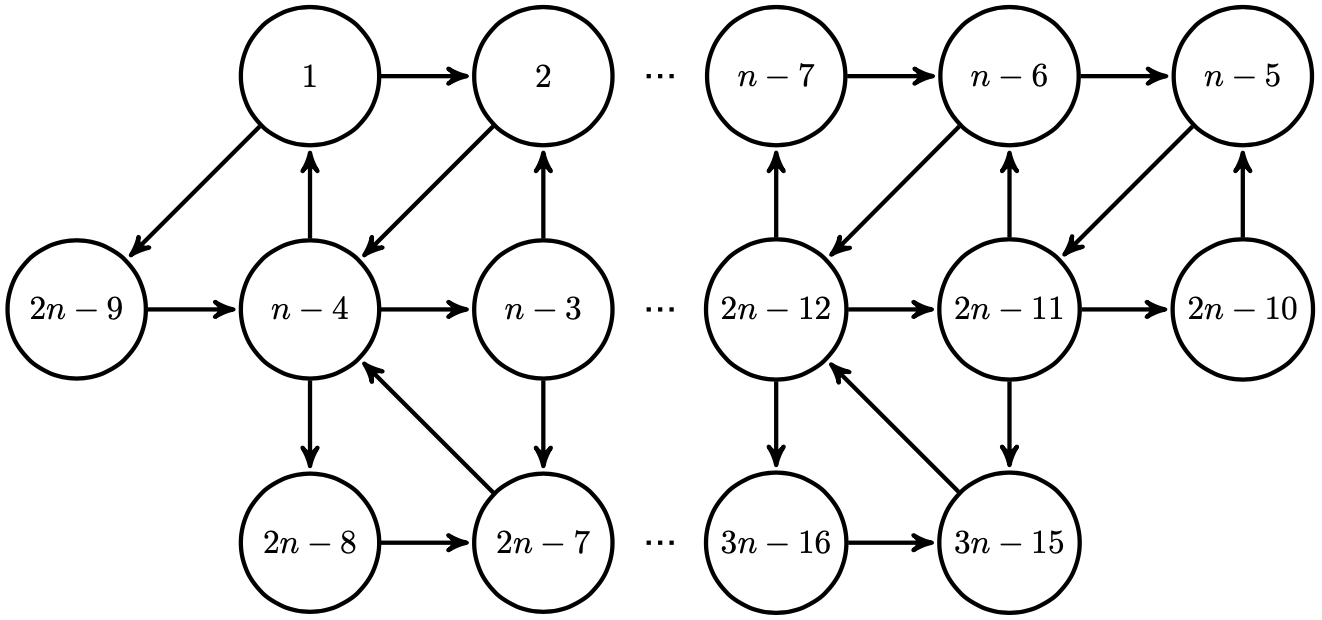
Figure 2: Left: Initial cluster of the ${\rm Gr}(4,n)$ cluster algebra, with respect to $\mathcal{X}$-coordinates. Right: Choice of cluster we begin mutating from so as to obtain all contiguous origin limits. The numbering of vertices is inherited from the initial cluster, where it starts at the top left, and increases first as we change columns, and then as we change rows.

Appendix A Tilted Cusp Anomalous Dimension

The tilted cusp anomalous dimension was introduced in ref. [10] using a one-parameter deformation of the BES equation [11]:

$$\Gamma_{\alpha}(g)=\Gamma(\alpha,g)=4g^{2}\left[1+\mathbb{K}(\alpha,g)\right]^{-1}_{11}\,,$$ (30)

where $\mathbb{K}(\alpha,g)$ is a semi-infinite matrix [50] with elements

$$\mathbb{K}(\alpha,g)_{ij} =4j(-1)^{ij+j}\cos{\alpha}\int\limits_{0}^{\infty}\frac{dt}{t}\frac{J_{i}(2gt)J_{j}(2gt)}{e^{t}-1}$$ (31)

$$\qquad\times\begin{cases}\cos{\alpha}\,,&\text{for}\ |i-j|\ \textrm{even}\\ \sin{\alpha}\,,&\text{otherwise}\end{cases}\,,$$

with $i,j\in\mathbb{N}$, and $J_{i}$ is the $i$-th Bessel function of the first kind. The ‘11’ subscript in eq. (30) refers to the 1,1 entry of the inverse of the matrix.

The deformation parameter $\alpha$ only enters the kernel in the cosine prefactors. The usual, undeformed BES equation is recovered when $\alpha=\pi/4$, $\Gamma_{\textrm{cusp}}(g)=\Gamma(\pi/4,g)$. The first few terms in the weak coupling expansion of $\Gamma_{\alpha}(g)$ are

$$\Gamma_{\alpha}(g) = 4g^{2}\Bigl{\{}1-4\zeta_{2}c^{2}g^{2}+8c^{2}(3+5c^{2})\zeta_{4}g^{4}$$ (32)

$$\hskip-11.38092pt\hbox{}-8c^{2}\Bigl{[}(25+42c^{2}+35c^{4})\zeta_{6}+4s^{2}(\zeta_{3})^{2}\Bigr{]}g^{6}$$

$$\hskip-11.38092pt\hbox{}+8c^{2}\Bigl{[}\Bigl{(}245+\tfrac{1273}{3}c^{2}+420c^{4}+\tfrac{700}{3}c^{6}\Bigr{)}\zeta_{8}$$

$$\hskip-2.84544pt\hbox{}+16\zeta_{3}(5\zeta_{5}+2\zeta_{2}\zeta_{3}c^{2})s^{2}\Bigr{]}g^{8}+{\cal O}(g^{10})\Bigr{\}}\,,~{}~{}~{}~{}$$

where $c=\cos\alpha$, $s=\sin\alpha$. We provide the values of $\Gamma_{\alpha}(g)$ through eight loops in the ancillary file Gamma_alpha.txt.

We remark that, despite the generically irrational trigonometric factors of $\cos\alpha$ and $\sin\alpha$ in the weak coupling expansion of an individual $\Gamma_{\alpha}$, in the full sum over angles, given by eq. (24), there are trigonometric identities that result in only rational coefficients multiplying the zeta values in the $c_{i}$, $d_{i}$ and $f_{i}$. The rationality of the coefficients can be made manifest to any loop order by an alternate evaluation of the contour integral in eq. (21), as we now explain. To any order in perturbation theory, $\mathcal{G}(z,g)$ has poles only at $z=0,\infty$. Therefore, the contour $C_{n}$ can be deformed away from the unit-circle poles of $\mathcal{S}_{n}(z)$, so that it encircles $z=0$ and $z=\infty$ instead. A symmetry under $z\leftrightarrow 1/z$ ensures that the $z=\infty$ residue equals the one at $z=0$, resulting in

$$R_{n}\overset{\textrm{PT}}{=}\oint\frac{dz}{2\pi iz}(z-1/z)\tilde{\mathcal{G}}(z,g)\mathcal{S}_{n}(z)\,,$$ (33)

with the contour going about $z=0$. From the perturbative expansion of $\mathcal{G}(z,g)$, which follows from eq. (32) by letting $c^{2}=-\tfrac{1}{4}(z+z^{-1}-2)$, $s^{2}=\tfrac{1}{4}(z+z^{-1}+2)$, it is clear that only rational coefficents will appear in the residue at $z=0$. The $z=0$ residue evaluation is also the simplest way to compare the master formula with perturbative data.

Appendix B Gram Determinant Constraints

At seven points, the seven cross ratios $u_{i}\equiv u_{i+1,i+4}$ (with all indices mod 7) obey a single Gram determinant constraint [35],

$$0 = 1+\biggl{[}-u_{1}+u_{1}u_{3}+u_{1}u_{4}+u_{1}u_{2}u_{5}-u_{1}u_{3}u_{5}-u_{1}^{2}u_{4}u_{5}-2u_{1}u_{2}u_{4}u_{5}+u_{1}u_{2}u_{3}u_{5}u_{6}+u_{1}^{2}u_{2}u_{4}u_{5}^{2}\ +\ \text{cyclic}\biggr{]}$$ (34)

$$+u_{1}u_{2}u_{3}u_{4}u_{5}u_{6}u_{7}\,.$$

At eight points, there are 12 cross ratios, eight $u_{i}\equiv u_{i+1,i+4}$ and four $v_{i}\equiv u_{i+1,i+5}$. They obey three independent Gram determinant constraints, which are provided in the ancillary file octagon_Gram.txt.

Appendix C Cluster Origins

After briefly reviewing the positive region and its cluster algebra structure, in this appendix we provide further details on how the latter can be used in order to classify origin limits.

The space of dual conformal $n$-particle kinematics of $\mathcal{N}=4$ SYM amplitudes is most conveniently described in terms of $n$ cyclically ordered momentum twistors $Z_{i}\in\mathbb{CP}^{3}$ [51], which can be assembled in a $4\times n$ matrix. The conventional Mandelstam invariants of eq. (1), for example, may be expressed in terms of certain maximal minors of this matrix,

$$x^{2}_{ij}\propto\langle i\!-\!1\,i\,j\!-\!1\,j\rangle\,,$$ (35)

$$\langle ijkl\rangle\equiv\langle Z_{i}Z_{j}Z_{k}Z_{l}\rangle=\det(Z_{i}Z_{j}Z_{k}Z_{l})\,,$$ (36)

up to proportionality factors that drop out from conformally invariant quantities. The positive region of this space [15, 16], which closely resembles the ${\rm Gr}(4,n)$ Grassmannian, is defined as the subspace where

$$\langle ijkl\rangle>0\qquad\forall\,\,i<j<k<l\,,$$ (37)

and it is naturally endowed with a cluster algebra structure, as is reviewed for example in ref. [24].

The building blocks of cluster algebras are cluster variables, which are grouped into overlapping subsets (the clusters) of the same size (the rank of the cluster algebra). Starting from an initial cluster, cluster algebras may be constructed recursively by a mutation operation on the cluster variables.

The cluster variable content and mutation rule of each cluster may be encoded in the vertices of a quiver, and the arrows connecting them, respectively. The initial quiver of the ${\rm Gr}(4,n)$ cluster algebra is depicted at the left of figure 2, where it is evident that the rank coincides with the dimension of the kinematic space, $3n-15$. While the original definition of cluster algebras by Fomin and Zelevinsky is with respect to so-called cluster $\mathcal{A}$-coordinates [12, 13], for the purposes of this paper we will be exclusively using the closely related cluster $\mathcal{X}$-coordinates introduced by Fock and Goncharov [14]. The reason is that for each cluster, these variables $\mathcal{X}_{i}$ correspond to the coordinates of a chart describing a compactification of the positive region (whose interior maps to $0<\mathcal{X}_{i}<\infty$). They are thus ideally suited for locating origin limits at its boundary.

The arrows between vertices $i$ and $j$ of the quiver define an antisymmetric exchange matrix $B$ with components

$$b_{ij}=(\#\ \text{arrows}\,\,i\to j)-(\#\ \text{arrows}\,\,j\to i)\,.$$ (38)

Upon mutation of the $k$-th vertex of the quiver, the $\mathcal{X}$-coordinates transform as

$$\mathcal{X}_{i}^{\prime}=\begin{cases}1/\mathcal{X}_{i}&k=i\,,\\ \mathcal{X}_{i}\bigl{(}1+\mathcal{X}_{k}^{{-\rm sgn}(b_{ki})}\bigr{)}^{-b_{ki}}&k\neq i\,,\end{cases}$$ (39)

whereas the components of the exchange matrix in the new cluster, $B^{\prime}$, are given by

$$b^{\prime}_{ij}=\begin{cases}-b_{ij}\quad&\text{for}\,i=k\,\text{or}\,j=k\\ b_{ij}+\left[-b_{ik}\right]_{+}b_{kj}+b_{ik}\left[b_{kj}\right]_{+}\quad&\text{otherwise}\end{cases}\,,$$ (40)

where $\left[x\right]_{+}=\max\left(0,x\right)$.

A (‘web’-)parametrization of the momentum twistor matrix in terms of the $\mathcal{X}$-coordinates of the initial cluster can be constructed algorithmically for any $n$ [29], see also [26, 28] for a simplified reformulation, and by virtue of the mutation rule (39) also for any other cluster. With the help of eqs. (1) and (35)–(36) we may then express all cross ratios in terms of them, and evaluate them at the vertex of the boundary polytope corresponding to each cluster, i.e. we let all its $\mathcal{X}$-coordinates $\mathcal{X}_{i}\to 0$. To illustrate this process with a particular example, the web-parametrization of the $4\times 6$ matrix of momentum twistors of the six-particle amplitude is

$$\left(\begin{array}[]{cccccc}1&0&0&0&-1&-1-\mathcal{X}_{1}-\mathcal{X}_{1}\mathcal{X}_{2}-\mathcal{X}_{1}\mathcal{X}_{2}\mathcal{X}_{3}\\ 0&1&0&0&1&1+\mathcal{X}_{1}+\mathcal{X}_{1}\mathcal{X}_{2}\\ 0&0&1&0&-1&-1-\mathcal{X}_{1}\\ 0&0&0&1&1&1\\ \end{array}\right)\,,$$ (41)

such that the cross ratios may be expressed in terms of the $\mathcal{X}$-coordinates of the initial cluster as

$$u_{1} =\frac{1}{1+\mathcal{X}_{2}+\mathcal{X}_{2}\mathcal{X}_{3}}\,,\quad u_{3}=\frac{\mathcal{X}_{1}\mathcal{X}_{2}}{1+\mathcal{X}_{1}+\mathcal{X}_{1}\mathcal{X}_{2}}\,,$$ (42)

$$u_{2} =\frac{\mathcal{X}_{2}\mathcal{X}_{3}}{\left(1+\mathcal{X}_{1}+\mathcal{X}_{1}\mathcal{X}_{2}\right)\left(1+\mathcal{X}_{2}+\mathcal{X}_{2}\mathcal{X}_{3}\right)}\,.$$

As is evident in this $n=6$ example, the initial cluster of figure 2 does not yield an origin point limit when $\mathcal{X}_{i}\to 0$. (We have defined these limits to have at least $3(n-5)$ cross ratios approaching zero, whereas this cluster is a corner of a multi-soft limit [52] with only $2(n-5)$ vanishing cross ratios.) Nevertheless, it is easy to show that $(n-5)!$ different origin limits may be obtained from it by mutating all the $\mathcal{X}$-coordinates of its middle row in all possible orders. In other words, these particular origins are $(n-5)$ mutations away from the initial cluster. This simple pattern has been inferred from the $n=6,7$ cases, and additionally checked up to $n=10$. A particularly simple choice of ordering is from left to right, which leads to the quiver at the right of figure 2 for any $n$.

Figure 3: Web of octagon origin clusters, color coded according to the origin classes 1, 2, 3, 4, 5, 6, 7, 8, 9 in table 1. It may be viewed as a half-sphere with two ${\color[rgb]{1,0,0}\rm O_{1}}$ at the north pole and with $\rm O_{9}$’s at the equator. The missing half-sphere is the parity image, which has been omitted for simplicity. Lines correspond to mutations between clusters, and same-colored vertices of different shape denote different directions of approach within each origin class. The lines between $\rm{\color[rgb]{1,0,0}O_{1}}$ and $\rm{\color[rgb]{1,.5,0}O_{2}}$ are not solid to indicate that the remainder function is not QL on them. They are dashed or dotted to distinguish which of the two overlapping $\rm{\color[rgb]{1,0,0}O_{1}}$ vertices they start from. The (super)line between the two $\rm{\color[rgb]{1,0,0}O_{1}}$’s is not visible.

Starting from this cluster, by further mutating we obtain all other contiguous clusters also corresponding to origin limits, as described in the main text. The exchange graph of a cluster algebra is a graph where its clusters are represented by vertices, and the mutations among them by edges. Restricting ourselves just to origin limit clusters and the mutations among them, this partial exchange graph for $n=8$ is depicted in figure 3. The edges of mutations between clusters of the same origin class sometimes amount to a change of a cross ratio by finite amount from 0 to 1 or vice versa, and sometimes by an infinitesimal amount. Namely they may connect different dihedral images among the same class, or two different directions of approach to the same strict limit. When approaching origin limits from the interior of the positive region, such that the amplitudes only exhibit QL behavior with respect to the cross ratios as described in the main text, the latter lines play no role, because they become points in the relevant cross ratio space. (Note that “direction of approach” is related to “speed of approach”, the behavior can depend on the Riemann sheet, and here we are on a Euclidean sheet. For example, on a physical scattering sheet, the limit $\mathcal{X}_{i}\to 0$ in eq. (42) corresponds to the multi-Regge limit, where the remainder function is definitely not QL, although it is QL there on the Euclidean sheet.) We may therefore coarsen the exchange graph by identifying clusters connected by such mutations. Further omitting dihedrally related vertices such that the higher-dimensional limits of table 2 appear only once, we finally arrive at the simplified graph of figure 1.

The complete data for the 1188 clusters of ${\rm Gr}(4,8)$ corresponding to origin limits of the eight-particle amplitude, including their exchange matrix and $\mathcal{X}$-coordinates, momentum twistor parametrization and values of the cross ratios in terms of these coordinates, as well as the adjacency matrix recording the mutation connectivity shown in figure 3, may be found in the attached ancillary file OctOriginClusterData.m.

Appendix D Octagon Cube 6789

On Cube 6789, five independent QL polynomials are allowed by continuity, dihedral symmetry, and FE conditions. Two of them are given in eqs. (12) and (13). The other three are lengthier and are given here:

$$P_{3}^{({\sc C})} =\sum_{i=1,2,4,5,6,8}l_{i}l_{i+1}-\sum_{i=2,3,6,7}l_{i}l_{i+2}$$

$$+(l_{2}-l_{3}+l_{6}-l_{7})\ell_{1}+(l_{3}+l_{7})\ell_{2}+(l_{4}+l_{8})\ell_{4}$$

$$-(\ell_{1}-\ell_{4})(\ell_{3}-\ell_{2})+\ell_{2}\ell_{3}\,,$$

$$P_{4}^{({\sc C})} =\sum_{i=1}^{8}l_{i}l_{i+2}+\sum_{i=1}^{4}(l_{i+2}+l_{i+3}+l_{i+6}+l_{i+7})\ell_{i}$$

$$-(l_{2}+l_{6})\ell_{1}-(l_{3}+l_{7})\ell_{2}-(l_{4}+l_{8})\ell_{4}$$

$$+2(\ell_{1}\ell_{3}+\ell_{2}\ell_{4})\,,$$

$$P_{5}^{({\sc C})} =\sum_{i=1,2,3,5,6,7}l_{i}l_{i+3}+\sum_{i=2,3,6,7}l_{i}l_{i+2}$$

$$+\sum_{i=1}^{4}(l_{i-1}+l_{i+3})\ell_{i}+\sum_{i=2}^{4}(l_{i+2}+l_{i+6})\ell_{i}$$

$$+\ell_{1}\ell_{3}+\ell_{2}\ell_{4}+\ell_{1}\ell_{2}+\ell_{2}\ell_{3}+\ell_{3}\ell_{4}\,.$$ (43)

We also give the coefficients $d_{i}$ appearing in eq. (11) through four loops,

$$d_{1} =d_{2}=-\tfrac{5}{2}g^{6}\zeta_{4}+g^{8}\left(\tfrac{413}{8}-2\zeta_{3}^{2}\zeta_{6}\right)+O(g^{10})\,,$$

$$d_{3} =g^{4}\zeta_{2}-\tfrac{37}{2}g^{6}\zeta_{4}+g^{8}\left(\tfrac{1975}{8}\zeta_{6}-2\zeta_{3}^{2}\right)+O(g^{10})\,,$$

$$d_{4} =d_{3}-\tfrac{35}{8}g^{8}\zeta_{6}+O(g^{10})\,,$$

$$d_{5} =O(g^{10})\,.$$ (44)

We give the values of the $d_{i}$ through eight loops in the ancillary file octagon_QL_coefs.txt.

Appendix E TBA Analysis

To construct the remainder function at the $n$-point origins, we need the TBA equations for the charged particles that trigger the QL behavior. Defining

$$f_{\pm,s}(z)=\int\frac{d\theta}{2\pi\cosh{(2\theta)}}z^{2i\theta/\pi}\ln{Y_{\pm 1,s}(\theta)}\,,$$ (45)

$$g_{\pm,s}(z)=\int\frac{d\theta}{2\pi\cosh{(2\theta)}}z^{2i\theta/\pi}\ln{\left[1+Y_{\pm 1,s}(\theta)\right]}\,,$$

and omitting the charge zero particles, eq. (14) becomes, in Fourier space,

$$f_{\pm,s}=\hat{I}_{\pm,s} +\frac{z}{1+z^{2}}(g_{+,s}+g_{-,s})$$ (46)

$$+\frac{z^{3}}{(1+z)(1+z^{2})}(g_{\pm,s+1}+g_{\pm,s-1})$$

$$-\frac{z}{(1+z)(1+z^{2})}(g_{\mp,s+1}+g_{\mp,s-1})\,,$$

for $s$ odd. The same equations hold for $s$ even, after replacing $z\rightarrow 1/z$ in each $z$-dependent coefficient. The driving terms are known functions of the OPE parameters, given by

$$\hat{I}_{\pm,s}=\frac{\sqrt{z}e_{\pm,s}(z)}{2(1+z)(1+z^{2})}\,,$$ (47)

with, for $s$ odd,

$$e_{\pm,s}=(\pm\varphi_{s}-\tau_{s}-\sigma_{s})-2\tau_{s}z+(\pm\varphi_{s}-\tau_{s}+\sigma_{s})z^{2}\,,$$ (48)

and similarly for $s$ even, with $\sigma_{s}\rightarrow-\sigma_{s}$.

When the chemical potentials and inverse temperatures are large, $|\varphi_{s}|,\tau_{s}\gg 1$, we set $g_{a,s}\rightarrow f_{a,s}$ in eq. (46) if the particles $(a,s)$ condense, and $g_{a,s}\rightarrow 0$ otherwise. The equations are then linear in $f$’s and are controlled by a matrix whose $z$-dependent coefficients may be read off from eq. (46). To be more concrete, for the choice $\Sigma_{n}=(h_{1},\ldots,h_{n-5})$, with $h_{s}$ the charge of the condensed particles in the $s$-th OPE channel, the TBA kernels can be packed into a tridiagonal $(n-5)\times(n-5)$ matrix,

$$1-K_{n}=\frac{1}{(1+z)(1+z^{2})}\left[\begin{array}[]{cccc}a_{1}&b_{1}&&\\ c_{1}&\ddots&\ddots&\\ &\ddots&\ddots&b_{n-6}\\ &&c_{n-6}&a_{n-5}\end{array}\right]\,,$$ (49)

with $a_{s}(z)=1+z^{3}$, $c_{s}(z)=z^{3}b_{s}(1/z)$, for $s\in\{1,\ldots,n-5\}$, and $b_{s}=\frac{1}{2}(1-h_{s}h_{s+1})z-\frac{1}{2}(1+h_{s}h_{s+1})z^{3}$, for $s$ odd, and similarly for $s$ even with $b_{s}\rightarrow c_{s}$.

The string integrand $\mathcal{S}_{n}(z)$ is a quadratic form in the OPE parameters, defined by contracting the inverse of $1-K_{n}(z)$ with the TBA sources,

$$\mathcal{S}_{n}(z)=\hat{I}(1/z)\cdot\left[1-K_{n}(z)\right]^{-1}\cdot\hat{I}(z)^{T}\,,$$ (50)

with $\hat{I}(z)\equiv(\hat{I}_{h_{1},1}(z),\ldots,\hat{I}_{h_{n-5},n-5}(z))$ and $T$ the transpose. Straightforward algebra with the matrix (49) allows us to cast $\mathcal{S}_{n}(z)$ into the canonical form (20) with $\mathcal{P}_{n}^{\Sigma}(z)$ encoding all the kinematic dependence. One may achieve further simplifications by factorizing $\mathcal{P}_{n}^{\Sigma}(z)$ on the support of the poles of $\mathcal{S}_{n}(z)$. Namely, one may show that

$$\mathcal{P}^{\Sigma}_{n}(z)\approx-\frac{1}{8z}(1+z^{3(n-4)})Q_{n}^{\Sigma}(z)Q_{n}^{\Sigma}(1/z)\,,$$ (51)

up to terms integrating to zero in the contour integral (21), with

$$Q_{n}^{\Sigma}(z)=\sum_{s=1}^{n-5}(-1)^{s+1}\frac{1-z^{3(n-4-s)}}{1-z^{3}}e_{s}(z)\prod_{i=1}^{s-1}b_{i}(z)\,,$$ (52)

and $e_{s}=e_{h_{s},s}$. The above function defines a polynomial in $z$, with coefficients depending linearly on $\{\sigma_{s},\tau_{s},\varphi_{s}\}_{s=1,\ldots,n-5}$. (The rhs of eq. (51) is a Laurent polynomial in $z$, unlike $\mathcal{P}_{n}^{\Sigma}(z)$ which is polynomial in $z$. Both polynomials obey $\mathcal{P}^{\Sigma}_{n}(z)=z^{3n-14}\mathcal{P}^{\Sigma}_{n}(1/z)$, which ensures the symmetry under $z\rightarrow 1/z$ of the string integrand (20).)

For illustration, when $n=6$,

$$\mathcal{S}_{6}(z)=\frac{\hat{I}(1/z)\hat{I}(z)}{1-K_{6}(z)}=\frac{z\mathcal{P}_{6}(z)}{(1+z)(1+z^{2})(1+z^{3})}\,,$$ (53)

with

$$\mathcal{P}_{6}(z) =\frac{z^{2}}{4}e_{1}(1/z)e_{1}(z)$$ (54)

$$=-\frac{(1+z^{6})}{8z}e_{1}(1/z)e_{1}(z)+\frac{(1+z^{3})^{2}}{8z}e_{1}(1/z)e_{1}(z)\,.$$

and $e_{1}(z)=-l_{1}+zl_{2}-z^{2}l_{3}$. We may discard the second term because it vanishes on the relevant poles, when $1+z^{3}=0$. (Poles at $z\pm i$ are cancelled by the vanishing of $\tilde{\Gamma}_{\pi/4}$.)

The polynomial $P^{\Sigma_{n}}_{\alpha}$ in $R_{n}=\sum_{\alpha}\tilde{\Gamma}_{\alpha}P_{\alpha}^{\Sigma_{n}}$ (eq. (24)) follows straightforwardly by evaluating the contour integral (21) around the unit-circle poles of the string integrand. Using eqs. (20) and (51), one finds

$$P^{\Sigma_{n}}_{\alpha}=-\frac{\cos{\alpha}\cos{(3\alpha)}}{12(n-4)\cos{(2\alpha)}}|Q^{\Sigma}_{n}(-e^{2i\alpha})|^{2}\,,$$ (55)

with $\alpha$ as in eq. (25). Simplifying further the expressions for $n=6,7$, using trigonometric identities, eqs. (26) and (28), one finds

$$P^{n=6}_{\alpha}=-\frac{1}{24}\bigg{|}\sum_{j=1}^{3}e^{2ij\alpha}l_{j}\bigg{|}^{2}\,,$$ (56)

with $\alpha=\{0,\pm\pi/3\}$, for the hexagon origin (2), and

$$P^{n=7}_{\alpha}=-\frac{\cos{\alpha}\cos{(3\alpha)}}{36\cos{(2\alpha)}}\bigg{|}\sum_{j=1}^{7}e^{2ij\alpha}l_{j}\bigg{|}^{2}\,,$$ (57)

with $\alpha=\{\pm\pi/18,\pm 5\pi/18,\pm 7\pi/18\}$, for Line 71 (4). One verifies the agreement with the general formulae reported earlier for these two cases.

Note that both the polynomial (55) and the tilted cusp anomalous dimension are symmetric under $\alpha\rightarrow-\alpha$. Hence, one may restrict the sum over angles to $0\leqslant\alpha\leqslant\pi/2$, including a factor of $2$ for all $\alpha\neq\{0,\pi/2\}$.

Notice also that $P_{\alpha}^{\Sigma_{n}}$ has a pole at $\alpha=\pi/4$, due to the cosine in the numerator in eq. (55). Still, the limit $\alpha\rightarrow\pi/4$ is well-defined at the level of the remainder function, since $\tilde{\Gamma}_{\alpha}=\Gamma_{\alpha}-\Gamma_{\pi/4}$ vanishes at this point. Namely,

$$\lim_{\alpha\rightarrow\pi/4}\frac{\tilde{\Gamma}_{\alpha}\cos{\alpha}\cos{(3\alpha)}}{\cos{(2\alpha)}}=\frac{\Gamma^{\prime}_{\pi/4}}{4}\,,$$ (58)

where $\Gamma^{\prime}_{\pi/4}\equiv\partial_{\alpha}\Gamma_{\alpha}|_{\alpha=\pi/4}=16\zeta_{2}g^{4}-256\zeta_{4}g^{6}+\ldots\,$. This limiting procedure is relevant whenever $n$ is a multiple of $4$, as one can see from the general expressions for the roots $\alpha$, see eq. (25). In particular, $\Gamma^{\prime}_{\pi/4}$ enters the description of the QL behavior of the octagon amplitude.

To get rid of the OPE parameters, one needs their mapping to the cross ratios in the limits of interest. The results for $n=6$ and $7$ are given in eqs. (26) and (28). Here we provide the missing information for $n=8$. One finds, when $|\varphi_{s}|\gg\tau_{s}\gg 1$, with $\sigma_{s}$ fixed,

$$u_{3}\approx e^{\tau_{3}-\sigma_{3}-|\varphi_{3}|}\,,\,\,\,u_{2}\approx e^{-2\tau_{3}}\,,\,\,\,u_{1}u_{4}v_{4}\approx e^{\tau_{3}+\sigma_{3}-|\varphi_{3}|}\,,$$ (59)

$$v_{1}\approx e^{\tau_{2}-\sigma_{2}-|\varphi_{2}|}\,,\,\,\,\,v_{2}\approx e^{-2\tau_{2}}\,,\,\,\,u_{4}u_{8}v_{3}v_{4}\approx e^{\tau_{2}+\sigma_{2}-|\varphi_{2}|}\,,$$

$$u_{7}\approx e^{\tau_{1}-\sigma_{1}-|\varphi_{1}|}\,,\,\,\,u_{6}\approx e^{-2\tau_{1}}\,,\,\,\,u_{5}u_{8}v_{4}\approx e^{\tau_{1}+\sigma_{1}-|\varphi_{1}|}\,,$$

with $u_{4}=u_{8}=v_{4}=1$ for $\Sigma_{8}=(+,+,+)$, $u_{8}=v_{4}=u_{1}+v_{3}=1$ for $\Sigma_{8}=(+,+,-)$, and $v_{3}=u_{4}+u_{5}=u_{1}+u_{8}=1$ for $\Sigma_{8}=(+,-,+)$. As alluded to before, these relations correspond, respectively, to the origin $\rm O_{9}$, a line between (images of) $\rm O_{3}$ and $\rm O_{4}$, and a square connecting (images of) $\rm O_{9},\rm O_{8}$ and two $\rm O_{7}$.

We may then compare the TBA prediction for $\Sigma_{8}=(+,+,+)$ with the perturbative ansatz (11) for ${\rm O_{9}}$, by taking the limit $u_{4},u_{8},v_{4}\rightarrow 1$ of Cube 6789 in table 2. The two expressions are seen to match perfectly. The associated coefficients $d_{i}$ are given to all loops by

$$d_{1} =-\frac{1}{96}(\Gamma^{\prime}_{\pi/4}+2\tilde{\Gamma}_{0}+4\tilde{\Gamma}_{\pi/3}+2\tilde{\Gamma}_{-})\,,$$ (60)

$$d_{2} =-\frac{1}{48}(\Gamma^{\prime}_{\pi/4}+2\tilde{\Gamma}_{-})\,,$$

$$d_{3} =-\frac{1}{48}(2\tilde{\Gamma}_{0}-2\tilde{\Gamma}_{\pi/3}+\tilde{\Gamma}_{+})\,,$$

$$d_{4} =-\frac{1}{48}(2\tilde{\Gamma}_{0}-\Gamma^{\prime}_{\pi/4}-2\tilde{\Gamma}_{\pi/3}+\tilde{\Gamma}_{-})\,,$$

$$d_{5} =-\frac{1}{48}(2\tilde{\Gamma}_{\pi/3}-2\tilde{\Gamma}_{0}+\tilde{\Gamma}_{+})\,,$$

where to save space we defined

$$\tilde{\Gamma}_{\pm}=(1+3^{\pm 1/2})\tilde{\Gamma}_{\pi/12}+(1-3^{\pm 1/2})\tilde{\Gamma}_{5\pi/12}\,.$$ (61)

As a cross check, one may verify that the exact same coefficients are obtained by matching the TBA predictions for $\Sigma_{8}=(+,+,-)$ and $\Sigma_{8}=(+,-,+)$ onto their corresponding line and surface. The $(+,+,-)$ result may be compared with the expressions for Pentagon 234 and Pentagon 345 in table 2, in the limit $u_{8},v_{4}\rightarrow 1$, using the ancillary file octagon_QL_formula.txt. The $(+,-,+)$ result may be matched with the formula for Cube 6789, after flipping $u_{i}\leftrightarrow u_{8-i},v_{1}\leftrightarrow v_{2},v_{3}\leftrightarrow v_{4}$ and taking the limit $v_{3}\rightarrow 1$.

Appendix F Superline

At $n=8$, we need an extra solution to the TBA equations to describe the super-origin $\rm O_{1}$, or, better yet, the Superline 1 connecting the two dihedral images of $\rm O_{1}$,

$$u_{1,\ldots,8}\rightarrow 0\,,\qquad v_{1}=1-v_{2}=v_{3}=1-v_{4}\,,$$ (62)

with $v_{1}\in[0,1]$. In terms of the OPE parameters, the line corresponds to

$$\tau_{1,3}\sim-\sigma_{1,3}\sim-\tfrac{1}{2}\sigma_{2}\sim\tfrac{1}{4}\varphi_{1}\sim-\tfrac{1}{4}\varphi_{3}\rightarrow+\infty\,,$$ (63)

with $\varphi_{2}$ and $\tau_{2}$ kept fixed. Here, the numerical coefficients indicate how the parameters scale with respect to one another, with e.g. $|\varphi_{1,3}|$ going to infinity 4 times faster than $\tau_{1,3}$. At first sight, one may think that this scaling is described by two large $Y$ functions, $Y_{1,1}$ and $Y_{-1,3}$, for the two large chemical potentials in eq. (63). This naive reasoning is not entirely correct however, because of the large $\sigma_{s}$ limit.

In order to find the right TBA description, one may draw inspiration from the analysis of the regular octagons [19]. The latter refers to a continuous family of cyclic-symmetric kinematics,

$$u_{1},\ldots,u_{8}=u\,,\qquad v_{1},\ldots,v_{4}=1/2\,,$$ (64)

labelled by the cross ratio $u\in(0,\infty)$. It intersects Superline 1 at its midpoint ($v_{1}=v_{2}$) when $u\rightarrow 0$. In the TBA setup, the cyclic kinematics is associated to a 1-parameter family of constant $Y$-function solutions, which can be constructed exactly for any $u$. The solution reads, in our notation,

$$Y_{0,1}=\frac{\sqrt{2Y_{-1,1}}}{1+Y_{-1,1}}=\frac{u}{1-u}\,,$$ (65)

with $Y_{a,s}=Y_{-a,4-s}$ and $Y_{1,1}Y_{-1,1}=Y_{1,2}Y_{0,1}=Y_{0,2}=1$. One concludes from it that four $Y$ functions are sent to infinity in the limit $u\rightarrow 0$, namely,

$$Y_{1,1}\,,Y_{1,2}\,,Y_{-1,2}\,,Y_{-1,3}\,,$$ (66)

assuming $Y_{1,1}>1$ for definiteness. Our working assumption is that the same system of four large $Y$ functions drives the QL behavior of the amplitude away from the cyclic point, all along Superline 1.

Allowing for a dependence on $\theta$ in the $Y$ functions (66) and going to Fourier space, one finds that the problem is controlled by the 4-dimensional square matrix

$$1-K_{8}(z)=\frac{1}{(1+z)(1+z^{2})}$$ (67)

$$\times\left[\begin{array}[]{cccc}1+z^{3}&-z^{3}&z&0\\ -1&1+z^{3}&-z(1+z)&z^{2}\\ z^{2}&-z(1+z)&1+z^{3}&-1\\ 0&z&-z^{3}&1+z^{3}\end{array}\right]\,,$$

with coefficients following directly from eq. (46). The string integrand $\mathcal{S}_{8}(z)$ is defined as usual,

$$\mathcal{S}_{8}(z)=\hat{I}(1/z)\cdot\left[1-K_{8}(z)\right]^{-1}\cdot\hat{I}(z)^{T}\,,$$ (68)

with $\hat{I}=(\hat{I}_{+,1},\hat{I}_{+,2},\hat{I}_{-,2},\hat{I}_{-,3})$. Straightforward algebra yields

$$\mathcal{S}_{8}(z)=\frac{z\mathcal{P}_{8}^{{\rm super}}(z)}{(1-z^{4})(1-z^{8})}\,,$$ (69)

where $\mathcal{P}_{8}^{{\rm super}}(z)=z^{10}\mathcal{P}_{8}^{{\rm super}}(1/z)$ is a polynomial of degree 10 in $z$ and is quadratic in the OPE parameters. One concludes that the singularities of $\mathcal{S}_{8}(z)$ lie on the unit circle, at the eight roots of unity, $1-z^{8}=0$, corresponding to $\alpha=\{0,\pm\pi/8,\pm\pi/4,\pm 3\pi/8,\pi/2\}$.

To eliminate the OPE parameters in the limit (63), one may use

$$u_{3}v_{1}\approx e^{\tau_{3}-\sigma_{3}+\varphi_{3}}\,,\,\,\,u_{2}\approx e^{-2\tau_{3}}\,,\,\,\,u_{1}u_{4}v_{2}\approx e^{\tau_{3}+\sigma_{3}+\varphi_{3}}\,,$$ (70)

$$u_{4}\approx e^{\tau_{2}+\sigma_{2}-\varphi_{2}}\,,\,\,\,\,\,\,v_{2}/v_{1}=e^{-2\tau_{2}}\,,\,\,\,\,\,\,u_{8}\approx e^{\tau_{2}+\sigma_{2}+\varphi_{2}}\,,$$

$$u_{7}v_{1}\approx e^{\tau_{1}-\sigma_{1}-\varphi_{1}}\,,\,\,\,u_{6}\approx e^{-2\tau_{1}}\,,\,\,\,u_{5}u_{8}v_{2}\approx e^{\tau_{1}+\sigma_{1}-\varphi_{1}}\,,$$

where all quantities are small, except $v_{2}/v_{1}=O(1)$. Plugging these relations inside $\mathcal{S}_{8}(z)$ and evaluating the master integral by residues around the unit-circle poles, one obtains the all-order remainder function on Superline 1 as a finite sum over angles. It reads,

$$R_{8}= -\sum_{\alpha}\frac{\tilde{\Gamma}_{\alpha}\cos{\alpha}\cos{(3\alpha)}}{16\cos{(2\alpha)}}\bigg{|}\sum_{j=1}^{8}e^{2ij\alpha}l_{j}\bigg{|}^{2}$$ (71)

$$-\frac{\tilde{\Gamma}_{0}}{32}(\sum_{j=1}^{8}l_{j}+2\ell_{1}+2\ell_{2})^{2}-\frac{\tilde{\Gamma}_{\pi/2}}{8}(\ell_{1}-\ell_{2})^{2}\,,$$

with the sum running over $\alpha=\{\pi/8,\pi/4,3\pi/8\}$ and with $l_{i}=\ln{u_{i}},\ell_{i}=\ln{v_{i}}$. Notice that only one term remains in the cyclic limit (64), namely, the one scaling with $\tilde{\Gamma}_{0}=\Gamma_{\textrm{oct}}-\Gamma_{\textrm{cusp}}$. The same happens at $n=6$, $R_{6}\sim-\tilde{\Gamma}_{0}\ln^{2}{(u_{1}u_{2}u_{3})}/24$, when approaching the origin along the diagonal $u_{1}=u_{2}=u_{3}$. It can be traced back to the fact that these limits are controlled by constant $Y$-function solutions.

Alternatively, we may expand the result over the basis of QL polynomials constructed with the baby amplitude bootstrap. The results match perfectly, with the coefficients

$$f_{1} =-\frac{1}{64}(\Gamma^{\prime}_{\pi/4}+2\tilde{\Gamma}_{0}+2\tilde{\Gamma}_{\pi/8}+2\tilde{\Gamma}_{3\pi/8})\,,\qquad f_{2} =-\frac{1}{8}(\tilde{\Gamma}_{0}+\tilde{\Gamma}_{\pi/2})\,,$$ (72)

$$f_{3} =-\frac{1}{32}(2\tilde{\Gamma}_{0}+\sqrt{2}\tilde{\Gamma}_{\pi/8}-\sqrt{2}\tilde{\Gamma}_{3\pi/8})\,,\qquad f_{4} =-\frac{1}{32}(2\tilde{\Gamma}_{0}-\Gamma^{\prime}_{\pi/4})\,,$$

$$f_{5} =-\frac{1}{32}(2\tilde{\Gamma}_{0}-\sqrt{2}\tilde{\Gamma}_{\pi/8}+\sqrt{2}\tilde{\Gamma}_{3\pi/8})\,.$$

We provide their explicit expressions at weak coupling through 8 loops in the ancillary file octagon_QL_coefs.txt.

References

- Alday and Maldacena [2007a] L. F. Alday and J. M. Maldacena, Gluon scattering amplitudes at strong coupling, JHEP 06, 064, arXiv:0705.0303 [hep-th] .
- Drummond et al. [2008] J. M. Drummond, G. P. Korchemsky, and E. Sokatchev, Conformal properties of four-gluon planar amplitudes and Wilson loops, Nucl. Phys. B795, 385 (2008), arXiv:0707.0243 [hep-th] .
- Brandhuber et al. [2008] A. Brandhuber, P. Heslop, and G. Travaglini, MHV amplitudes in N=4 super Yang-Mills and Wilson loops, Nucl. Phys. B794, 231 (2008), arXiv:0707.1153 [hep-th] .
- Drummond et al. [2010] J. M. Drummond, J. Henn, G. P. Korchemsky, and E. Sokatchev, Conformal Ward identities for Wilson loops and a test of the duality with gluon amplitudes, Nucl. Phys. B826, 337 (2010), arXiv:0712.1223 [hep-th] .
- Alday et al. [2011a] L. F. Alday, D. Gaiotto, J. Maldacena, A. Sever, and P. Vieira, An Operator Product Expansion for Polygonal null Wilson Loops, JHEP 04, 088, arXiv:1006.2788 [hep-th] .
- Basso et al. [2013] B. Basso, A. Sever, and P. Vieira, Spacetime and Flux Tube S-Matrices at Finite Coupling for N=4 Supersymmetric Yang-Mills Theory, Phys. Rev. Lett. 111, 091602 (2013), arXiv:1303.1396 [hep-th] .
- Gubser et al. [2002] S. S. Gubser, I. R. Klebanov, and A. M. Polyakov, A Semiclassical limit of the gauge / string correspondence, Nucl. Phys. B636, 99 (2002), arXiv:hep-th/0204051 [hep-th] .
- Alday and Maldacena [2007b] L. F. Alday and J. M. Maldacena, Comments on operators with large spin, JHEP 11, 019, arXiv:0708.0672 [hep-th] .
- Caron-Huot et al. [2019] S. Caron-Huot, L. J. Dixon, F. Dulat, M. von Hippel, A. J. McLeod, and G. Papathanasiou, Six-Gluon amplitudes in planar = 4 super-Yang-Mills theory at six and seven loops, JHEP 08, 016, arXiv:1903.10890 [hep-th] .
- Basso et al. [2020] B. Basso, L. J. Dixon, and G. Papathanasiou, Origin of the Six-Gluon Amplitude in Planar Supersymmetric Yang-Mills Theory, Phys. Rev. Lett. 124, 161603 (2020), arXiv:2001.05460 [hep-th] .
- Beisert et al. [2007] N. Beisert, B. Eden, and M. Staudacher, Transcendentality and Crossing, J. Stat. Mech. 0701, P01021 (2007), arXiv:hep-th/0610251 [hep-th] .
- Fomin and Zelevinsky [2002] S. Fomin and A. Zelevinsky, Cluster Algebras I: Foundations, Journal of the American Mathematical Society 15, 497 (2002), arXiv:math/0104151 [math.RT] .
- Fomin and Zelevinsky [2003] S. Fomin and A. Zelevinsky, Cluster algebras II: Finite type classification, Inventiones mathematicae 154, 63 (2003), arXiv:math/0208229 [math.RA] .
- Fock and Goncharov [2009] V. V. Fock and A. B. Goncharov, Cluster ensembles, quantization and the dilogarithm, Ann. Sci. Éc. Norm. Supér. (4) 42, 865 (2009), arXiv:math/0311245 [math.AG] .
- Arkani-Hamed et al. [2016] N. Arkani-Hamed, J. L. Bourjaily, F. Cachazo, A. B. Goncharov, A. Postnikov, and J. Trnka, Grassmannian Geometry of Scattering Amplitudes (Cambridge University Press, 2016) arXiv:1212.5605 [hep-th] .
- Golden et al. [2014] J. Golden, A. B. Goncharov, M. Spradlin, C. Vergu, and A. Volovich, Motivic Amplitudes and Cluster Coordinates, JHEP 01, 091, arXiv:1305.1617 [hep-th] .
- Fock and Goncharov [2016] V. V. Fock and A. B. Goncharov, Cluster poisson varieties at infinity, Selecta Mathematica 22, 2569 (2016).
- Alday et al. [2011b] L. F. Alday, D. Gaiotto, and J. Maldacena, Thermodynamic Bubble Ansatz, JHEP 09, 032, arXiv:0911.4708 [hep-th] .
- Alday et al. [2010] L. F. Alday, J. Maldacena, A. Sever, and P. Vieira, Y-system for Scattering Amplitudes, J. Phys. A 43, 485401 (2010), arXiv:1002.2459 [hep-th] .
- Bonini et al. [2016] A. Bonini, D. Fioravanti, S. Piscaglia, and M. Rossi, Strong Wilson polygons from the lodge of free and bound mesons, JHEP 04, 029, arXiv:1511.05851 [hep-th] .
- Drummond et al. [2007] J. Drummond, J. Henn, V. Smirnov, and E. Sokatchev, Magic identities for conformal four-point integrals, JHEP 01, 064, arXiv:hep-th/0607160 .
- Arkani-Hamed et al. [2021a] N. Arkani-Hamed, T. Lam, and M. Spradlin, Non-perturbative geometries for planar = 4 SYM amplitudes, JHEP 03, 065, arXiv:1912.08222 [hep-th] .
- Scott [2003] J. S. Scott, Grassmannians and Cluster Algebras, arXiv Mathematics e-prints , math/0311148 (2003), arXiv:math/0311148 [math.CO] .
- Papathanasiou [2022] G. Papathanasiou, The SAGEX Review on Scattering Amplitudes, Chapter 5: Analytic Bootstraps for Scattering Amplitudes and Beyond, (2022), arXiv:2203.13016 [hep-th] .
- Drummond et al. [2020] J. Drummond, J. Foster, Ö. Gürdoğan, and C. Kalousios, Tropical Grassmannians, cluster algebras and scattering amplitudes, JHEP 04, 146, arXiv:1907.01053 [hep-th] .
- Drummond et al. [2021] J. Drummond, J. Foster, Ö. Gürdoğan, and C. Kalousios, Algebraic singularities of scattering amplitudes from tropical geometry, JHEP 04, 002, arXiv:1912.08217 [hep-th] .
- Henke and Papathanasiou [2020] N. Henke and G. Papathanasiou, How tropical are seven- and eight-particle amplitudes?, JHEP 08, 005, arXiv:1912.08254 [hep-th] .
- Henke and Papathanasiou [2021] N. Henke and G. Papathanasiou, Singularities of eight- and nine-particle amplitudes from cluster algebras and tropical geometry, JHEP 10, 007, arXiv:2106.01392 [hep-th] .
- Speyer and Williams [2005] D. Speyer and L. Williams, The Tropical Totally Positive Grassmannian, Journal of Algebraic Combinatorics 22, 189 (2005), arXiv:math/0312297 [math.CO] .
- Arkani-Hamed et al. [2021b] N. Arkani-Hamed, S. He, and T. Lam, Stringy canonical forms, JHEP 02, 069, arXiv:1912.08707 [hep-th] .
- Note [1] The polytope is a truncated triangular bipyramid, but if we collapse its vertices that correspond to the same points in cross-ratio space, we get a cube in both cases.
- Bern et al. [2005] Z. Bern, L. J. Dixon, and V. A. Smirnov, Iteration of planar amplitudes in maximally supersymmetric Yang-Mills theory at three loops and beyond, Phys. Rev. D72, 085001 (2005), arXiv:hep-th/0505205 [hep-th] .
- Bern et al. [2008] Z. Bern, L. J. Dixon, D. A. Kosower, R. Roiban, M. Spradlin, C. Vergu, and A. Volovich, The Two-Loop Six-Gluon MHV Amplitude in Maximally Supersymmetric Yang-Mills Theory, Phys. Rev. D78, 045007 (2008), arXiv:0803.1465 [hep-th] .
- Drummond et al. [2009] J. M. Drummond, J. Henn, G. P. Korchemsky, and E. Sokatchev, Hexagon Wilson loop = six-gluon MHV amplitude, Nucl. Phys. B815, 142 (2009), arXiv:0803.1466 [hep-th] .
- Dixon and Liu [2020] L. J. Dixon and Y.-T. Liu, Lifting Heptagon Symbols to Functions, JHEP 10, 031, arXiv:2007.12966 [hep-th] .
- Caron-Huot and He [2012] S. Caron-Huot and S. He, Jumpstarting the All-Loop S-Matrix of Planar N=4 Super Yang-Mills, JHEP 07, 174, arXiv:1112.1060 [hep-th] .
- Goncharov et al. [2010] A. B. Goncharov, M. Spradlin, C. Vergu, and A. Volovich, Classical Polylogarithms for Amplitudes and Wilson Loops, Phys. Rev. Lett. 105, 151605 (2010), arXiv:1006.5703 [hep-th] .
- Drummond et al. [2015] J. M. Drummond, G. Papathanasiou, and M. Spradlin, A Symbol of Uniqueness: The Cluster Bootstrap for the 3-Loop MHV Heptagon, JHEP 03, 072, arXiv:1412.3763 [hep-th] .
- Caron-Huot [2011] S. Caron-Huot, Superconformal symmetry and two-loop amplitudes in planar N=4 super Yang-Mills, JHEP 12, 066, arXiv:1105.5606 [hep-th] .
- Li and Zhang [2021] Z. Li and C. Zhang, The three-loop MHV octagon from equations, JHEP 12, 113, arXiv:2110.00350 [hep-th] .
- Note [2] We thank A. McLeod for confirming one of these limits using results in ref. [53].
- Note [3] We have checked that the full one-loop amplitude, including all non-dual-conformal terms associated with infrared divergences, is QL for all origins. This suffices to show that the logarithm of the full amplitude is QL. The nontrivial statement is that the dilogarithms of generic arguments cancel out, which requires the use of the five-term dilog identity for Pentagons 234 and 345.
- Bena et al. [2004] I. Bena, J. Polchinski, and R. Roiban, Hidden symmetries of the AdS(5) x S**5 superstring, Phys. Rev. D 69, 046002 (2004), arXiv:hep-th/0305116 .
- Ito et al. [2018] K. Ito, Y. Satoh, and J. Suzuki, MHV amplitudes at strong coupling and linearized TBA equations, JHEP 08, 002, arXiv:1805.07556 [hep-th] .
- Basso et al. [2014] B. Basso, A. Sever, and P. Vieira, Space-time S-matrix and Flux tube S-matrix II. Extracting and Matching Data, JHEP 01, 008, arXiv:1306.2058 [hep-th] .
- Coronado [2018] F. Coronado, Bootstrapping the simplest correlator in planar SYM at all loops, (2018), arXiv:1811.03282 [hep-th] .
- Kostov et al. [2019] I. Kostov, V. B. Petkova, and D. Serban, The Octagon as a Determinant, JHEP 11, 178, arXiv:1905.11467 [hep-th] .
- Belitsky and Korchemsky [2019] A. V. Belitsky and G. P. Korchemsky, Exact null octagon, (2019), arXiv:1907.13131 [hep-th] .
- Bercini et al. [2021] C. Bercini, V. Gonçalves, and P. Vieira, Light-Cone Bootstrap of Higher Point Functions and Wilson Loop Duality, Phys. Rev. Lett. 126, 121603 (2021), arXiv:2008.10407 [hep-th] .
- Benna et al. [2007] M. K. Benna, S. Benvenuti, I. R. Klebanov, and A. Scardicchio, A Test of the AdS/CFT correspondence using high-spin operators, Phys. Rev. Lett. 98, 131603 (2007), arXiv:hep-th/0611135 [hep-th] .
- Hodges [2013] A. Hodges, Eliminating spurious poles from gauge-theoretic amplitudes, JHEP 05, 135, arXiv:0905.1473 [hep-th] .
- Del Duca et al. [2016] V. Del Duca, S. Druc, J. Drummond, C. Duhr, F. Dulat, R. Marzucca, G. Papathanasiou, and B. Verbeek, Multi-Regge kinematics and the moduli space of Riemann spheres with marked points, JHEP 08, 152, arXiv:1606.08807 [hep-th] .
- Golden and McLeod [2021] J. Golden and A. J. McLeod, The two-loop remainder function for eight and nine particles, JHEP 06, 142, arXiv:2104.14194 [hep-th] .