DOLCE: A Model-Based Probabilistic Diffusion Framework
for Limited-Angle CT Reconstruction

Abstract

Limited-Angle Computed Tomography (LACT) is a non-destructive evaluation technique used in a variety of applications ranging from security to medicine. The limited angle coverage in LACT is often a dominant source of severe artifacts in the reconstructed images, making it a challenging inverse problem. We present DOLCE, a new deep model-based framework for LACT that uses a conditional diffusion model as an image prior. Diffusion models are a recent class of deep generative models that are relatively easy to train due to their implementation as image denoisers. DOLCE can form high-quality images from severely under-sampled data by integrating data-consistency updates with the sampling updates of a diffusion model, which is conditioned on the transformed limited-angle data. We show through extensive experimentation on several challenging real LACT datasets that, the same pre-trained DOLCE model achieves the SOTA performance on drastically different types of images. Additionally, we show that, unlike standard LACT reconstruction methods, DOLCE naturally enables the quantification of the reconstruction uncertainty by generating multiple samples consistent with the measured data.

1 Introduction

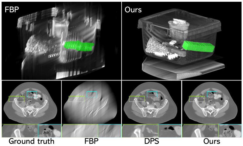
Figure 1: We show that the same pre-trained DOLCE model can reconstruct distinct CT images such as checked-in luggage [57] and human body [52]. Top: 3D rendering of a luggage from its 2D slices reconstructed using DOLCE on the limited-angle data containing just one-third of the views (0-60^∘). Note how our method preserves the 3D edges, enabling a successful recovery of the object geometries. Bottom: Comparison of DOLCE on a medical dataset with DPS, which is a SOTA method for solving imaging inverse problems using unconditional diffusion models [13]. See Section 5 for the complete set of experimental results.

Computed Tomography (CT) is one of the most widely-used imaging modalities with applications in medical diagnosis, industrial non-destructive testing, and security [77, 18, 78, 81]. In a typical parallel-beam CT imaging system, the x-ray measurements obtained from all viewing angles are combined to reconstruct a cross-sectional image of a 3D object [41]. Conventional reconstruction methods such as Filtered Back Projection (FBP) can produce high-quality CT images given a complete set of projection data, but completely fail under more ill-posed scenarios such as Limited-Angle CT (LACT), where projections from only a limited range of angles can be acquired (i.e., $0\leq\theta\leq\theta_{\text{max}}$ with $\theta_{\text{max}}<\pi$) [3, 58, 39, 11, 54]. A typical solution to this inverse problem is model-based optimization that integrates a forward model characterizing the imaging system and a regularizer imposing priors on the unknown image. While there has been significant progress in algorithms that leverage sophisticated image priors (e.g., transform-domain sparsity, self-similarity, and learned dictionaries) [21, 20, 45, 17], the focus in the area has recently shifted to deep learning (DL).

Deep Learning for CT: A traditional DL reconstruction involves training a convolutional neural network (CNN) architecture, such as U-Net [60], to directly perform a regularized inversion of the forward model by exploiting redundancies in the training data [40, 37, 27, 29, 88, 2, 92, 91]. Model-based DL (MBDL) is another popular reconstruction strategy that seeks to explicitly use the knowledge of the forward model by integrating a CNN into a model-based algorithm. Popular MBDL frameworks include Plug-and-Play Priors (PnP) [74, 59], which use pre-trained deep denoisers as image priors [69, 53, 90], and Deep Unfolding [25, 1, 48, 24, 94, 35], which interpret the iterations of a model-based algorithm as layers of a CNN to perform end-to-end supervised training. Other DL strategies used in CT reconstruction include dual-domain learning [72, 93], deep internal learning [89, 61, 73], and measurement synthesis learning [46, 47, 71]. Despite the rich literature on tomographic imaging, the reconstruction of high-quality images with sharp edges remains a well-known challenge, particularly when the acquired data is missing a large-range of angles (i.e., $\theta_{\text{max}}\leq 90^{\circ}$). Furthermore, most prior work in the area has focused on methods that can only produce point estimates without any quantification of the reconstruction uncertainty, which can be essential in critical applications such as healthcare or security.

Proposed Work: We present Diffusion Probabilistic Limited-Angle CT Reconstruction (DOLCE), a conditional generative model for LACT, which can generate multiple diverse, yet high-quality, reconstructions from a given limited-angle data. Inspired by the recent successes of Denoising Diffusion Probabilistic Models (DDPM) [63, 19] and denoising score matching [65, 66], we design DOLCE as a “repeated-refinement” conditional diffusion model. Specifically, DOLCE trains a stochastic sampler conditioned on noisy seed reconstructions obtained using transformed limited-angle sinograms. To boost the imaging quality further, DOLCE imposes an additional data-consistency step at every iteration after the sampling-update step. DOLCE can thus be viewed as a method for transforming a standard normal distribution into an empirical data distribution through a sequence of refinement steps, while integrating physical forward models and learned stochastic samplers (see Fig. 2).

We demonstrate several unique features of DOLCE compared to the prior work through extensive experimentation on two real-world LACT datasets. We first show that, on both applications, DOLCE achieves the state-of-the-art (SOTA) performance by directly producing high-resolution $512\times 512$ images across a range of limited-angle scenarios ($\theta_{\text{max}}\in\{60^{\circ},90^{\circ},120^{\circ}\}$). Next, we make an interesting finding that the same pre-trained DOLCE model can be effective on LACT from significantly different data distributions, such as images of human body and of checked-in luggage, enabling highly generalizable CT reconstruction networks for the first time. Finally, we show how the diverse realizations produced by DOLCE (from a given sinogram) can enable meaningful uncertainty quantification [43]. Notably, we find the variances estimated by DOLCE to be well calibrated, i.e., consistent with the true reconstruction errors. In short, DOLCE is the first model-based probabilistic diffusion framework for LACT that achieves SOTA performance and enables systematic uncertainty characterization.

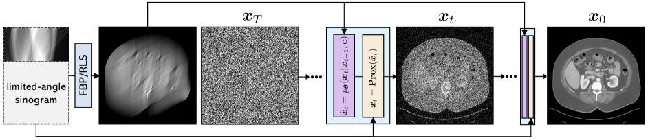
Figure 2: Overview of the proposed approach. Starting from the Gaussian noise ${\bm{x}}_{T}$, we sample an image ${\bm{x}}_{0}$ from the posterior by solving the reverse process of conditional denoising diffusion model, alternating between the denoising-update step and the data-consistency step.

Our main contributions can be summarized as follows:

1. We propose DOLCE as the first conditional diffusion model for the recovery of high-quality CT images from limited-angle sinograms.

2. We show that DOLCE is effective across two real-world datasets: checked-in luggage and medical-image datasets. DOLCE achieves a PSNR improvement of at least 3 dB over ILVR [12] and DPS [13], two SOTA diffusion models for inverse problems.

3. We use DOLCE to provide uncertainty maps for the reconstructed LACT images. The uncertainty estimates are reflective of the true reconstruction errors.

4. Using a 3D segmentation experiment, we show the effectiveness of DOLCE in recovering the geometric structure and sharp edges in high-resolution images, even in severely ill-posed settings.

2 Related Work

Tomographic Image Reconstruction. Traditional analytic algorithms such as FBP are commonly used for CT reconstruction. However, FBP produces inaccurate reconstructions with noise and artifacts when the imaging conditions are highly ill-posed such as in limited angle or sparse-views scenarios. Iterative methods are a popular alternative for tomographic reconstruction. Earlier works such as Algebraic Reconstruction Techniques (ART) [26], solve a discrete formulation of the reconstruction problem. These approaches can be combined with regularizers in an optimization framework, resulting in model-based iterative reconstruction (MBIR) algorithms [54, 38, 87, 76, 6, 75]. MBIR optimizes the reconstruction solution such that it best fits to the forward model, which captures the measurement physics and noise statistics, and a prior model for the object.

Recent DL-based methods adopt an end-to-end approach where a deep network architecture is trained in a supervised fashion to directly produce a point estimate [40, 37, 2, 22, 91, 34, 8, 92, 24]. For example,  [24, 10, 94, 48, 35] propose to unfold an iterative algorithm and train it end-to-end as a deep neural network. This enables integration of the physical information into the architecture in the form of data-consistency blocks that are combined with trainable CNN regularizers. Deep internal learning methods are alternates for tomographic reconstruction that explore the internal information of the test signal for learning a neural network prior without using any external data [23, 89, 61, 4, 84]. A related family of denoising-driven approaches known as PnP algorithms represents alternative to traditional DL methods by combining iterative model-based algorithms with deep denoisers as priors and have been shown to be effective in various forms of tomographic imaging [51, 80, 70, 49].

Diffusion Models in Imaging. Denoising diffusion models [32, 19, 44] and score-based models [65, 66, 68] are two related classes of generative models that were shown to achieve the SOTA performance in unconditional image generation. Despite being discovered independently, both classes are often referred to as diffusion models due to their similarity [36, 44]. Diffusion models are trained to model the Markov transition from a simple distribution to the data distribution, enabling the generation of samples through sequential stochastic transitions. Apart from unconditional image generation, diffusion models have recently been applied to conditional image generation, including super-resolution [12, 63, 14], sparse-CT reconstruction [67, 14], MRI reconstruction [14, 16, 86], and phase-retrieval [13]. For example, one line of work has focused on designing diffusion models suitable for specific image reconstruction tasks [63, 85, 16]. Another line of work has focused on keeping the training of a diffusion model intact, and only modify the inference procedure to enable sampling from a conditional distribution [12, 42, 13, 67, 14, 15, 50]. These methods can be thought of as solving different image reconstruction tasks by leveraging the learned score function as a generative prior of the data distribution. However, for the severely ill-posed LACT reconstruction, the current SOTA diffusion models often fail to generate images with desired semantics and accurate details (see Section 5). The proposed DOLCE method addresses this issue by integrating conditional learning and model-based inference for SOTA reconstruction in LACT.

3 Preliminaries

Inverse Problems. The problem of LACT reconstruction can be formulated as a linear inverse problem involving the recovery of an image ${\bm{x}}\in\mathbb{R}^{n}$ from incomplete measurements ${\bm{y}}={\bm{A}}{\bm{x}}$, where ${\bm{A}}\in\mathbb{R}^{m\times n}$ is the measurement operator modeling the observation process. Recovering ${\bm{x}}$ from ${\bm{y}}$ in LACT is highly ill-posed, often requiring addition assumptions on the unknown ${\bm{x}}$. From the Bayesian statistical perspective, the estimation can be viewed as sampling from the posterior distribution $p({\bm{x}}|{\bm{y}})$. One can also compute point estimates of ${\bm{x}}$ using the maximum-a-posteriori probability (MAP) $\mathop{\mathrm{arg\,max}}{p({\bm{x}}|{\bm{y}})}$ or minimum mean square error (MMSE) $\mathbb{E}[{\bm{x}}|{\bm{y}}]$ estimators.

Denoising Diffusion Probabilistic Models. DDPM refers to generative models that learn a target data distribution from samples [32, 64]. DDPM consists of two Markov processes: the fixed forward process and the learning-based reverse process. The forward process starts from a sample of a clean image ${\bm{x}}_{0}\sim q({\bm{x}}_{0})$ and gradually adds Gaussian noise according to the following transition probability:

$$q({\bm{x}}_{t}|{\bm{x}}_{t-1}):={\mathcal{N}}({\bm{x}}_{t};\sqrt{1-\beta_{t}}{\bm{x}}_{t-1},\beta_{t}{\mathbf{I}}),$$ (1)

where ${\mathcal{N}}(\cdot)$ denotes the Gaussian pdf, $\beta_{1:T}$ refers to a variance schedule subject to $\beta_{t}\in(0,1)$ for all $t=1,\cdots,T$. The latent variables ${\bm{x}}_{1:T}$ have the same dimensionality as the original image sample ${\bm{x}}_{0}\in\mathbb{R}^{n}$, and latent ${\bm{x}}_{T}$ is nearly an isotropic Gaussian distribution for large enough $T$ and a properly selected $\beta_{t}$ schedule. By parameter change of $\alpha_{t}:=1-\beta_{t}$ and $\bar{\alpha}_{t}=\Pi_{s=1}^{t}\alpha_{s}$, we can write ${\bm{x}}_{t}$ as a linear combination of noise ${\bm{\epsilon}}$ and ${\bm{x}}_{0}$

$${\bm{x}}_{t}=\sqrt{\bar{\alpha}_{t}}{\bm{x}}_{0}+\sqrt{1-\bar{\alpha}_{t}}{\bm{\epsilon}},$$ (2)

where ${\bm{\epsilon}}\sim{\mathcal{N}}(0,{\mathbf{I}})$. This allows a closed-form expression for the marginal distribution for sampling ${\bm{x}}_{t}$ given ${\bm{x}}_{0}$

$$q({\bm{x}}_{t}|{\bm{x}}_{0}):={\mathcal{N}}({\bm{x}}_{t};\sqrt{\bar{\alpha}_{t}}{\bm{x}}_{0},(1-\bar{\alpha}_{t}){\mathbf{I}}).$$ (3)

Improved Reverse Process. Since the reverse process $q({\bm{x}}_{t-1}|{\bm{x}}_{t})$ depends on the entire data distribution and is not tractable, we can learn the parameterized Gaussian transitions $p_{{\bm{\theta}}}({\bm{x}}_{t-1}|{\bm{x}}_{t})$ using a neural network as follows:

$$p_{{\bm{\theta}}}({\bm{x}}_{t-1}|{\bm{x}}_{t})={\mathcal{N}}({\bm{x}}_{t-1};\mu_{{\bm{\theta}}}({\bm{x}}_{t},t),\sigma_{t}^{2}{\mathbf{I}}),$$ (4)

where $\mu_{{\bm{\theta}}}({\bm{x}}_{t},t)$ refers to the learned mean. It is worth noting that originally Ho et al. [32] set the variance $\sigma_{t}$ to a fixed constant value. However, subsequent works [56, 19] proved the improved generation efficiency by using learned variance $\sigma_{t}^{2}\,\coloneqq\,\sigma^{2}_{{\bm{\theta}}}({\bm{x}}_{t},t)$, which we also adopt. In particular, the variances $\sigma_{{\bm{\theta}}}({\bm{x}}_{t},t)\,\coloneqq\,\exp(v\log\beta_{t}+(1-v)\log\tilde{\beta}_{t})$, correspond to the output of the neural network and $\tilde{\beta}_{t}$ refers to the lower bounds for the reverse process variances [32]. We use a single neural network with two separate output heads to estimate the mean and variance of this Gaussian distribution jointly. Practically, one can relate ${\bm{x}}_{t}$ and ${\bm{x}}_{0}$ via Equation (2) and (3) by decomposing $\mu_{{\bm{\theta}}}$ into a linear combination of ${\bm{x}}_{t}$ and the noise approximation $\epsilon_{{\bm{\theta}}}$. More specifically, we have ${\bm{x}}_{t}=\sqrt{\bar{\alpha}}{\bm{x}}_{0}+\sqrt{(1-\bar{\alpha})}{\bm{\epsilon}}$ for ${\bm{\epsilon}}\sim{\mathcal{N}}(0,{\mathbf{I}})$ and can train the network $\epsilon_{{\bm{\theta}}}$ as a denoiser to predict ${\bm{\epsilon}}$. During sampling, we can use simple substitution to derive $\mu_{{\bm{\theta}}}({\bm{x}}_{t},t)$ from network prediction $\epsilon_{{\bm{\theta}}}({\bm{x}}_{t},t)$

$${\bm{x}}_{t-1}=\frac{1}{\sqrt{\alpha_{t}}}\bigg{(}{\bm{x}}_{t}-\frac{1-\alpha_{t}}{\sqrt{1-\bar{\alpha}_{t}}}\epsilon_{{\bm{\theta}}}({\bm{x}}_{t},t)\bigg{)}+\sigma_{t}{\bm{z}},$$ (5)

where ${\bm{z}}\sim{\mathcal{N}}(0,{\mathbf{I}})$. Since the model learns the reverse Markov Chain running backward in time from ${\bm{x}}_{T}$ to ${\bm{x}}_{0}$, estimating clean image ${\bm{x}}_{0}$ from partially noisy image ${\bm{x}}_{t}$, we refer to this as the  reverse process.

4 Proposed Approach: DOLCE

In this section, we present our proposed approach for LACT, and describe the training and testing strategies. An overview of DOLCE is provided in Fig. 2. Our goal here is to reconstruct full-view images sampled from the conditional distribution $p({\bm{x}}_{0}|{\bm{c}})$, where the condition ${\bm{c}}$ is obtained from a limited angle sinogram. Specifically, we make the neural network accept ${\bm{c}}$ as the conditioning input. Note that while related ideas have been considered in other applications, such as image blurring [82] and super-resolution [63], our work is the first to adopt conditional sampling for CT reconstruction. This way, the iterative denoising procedure becomes dependent on ${\bm{c}}$ and the conditional diffusion model can generate a target image ${\bm{x}}_{0}$ in $T$ refinement steps. Starting from step $T$, each Markov transition under the condition ${\bm{c}}$ is approximated as follows:

$$\quad\quad p_{{\bm{\theta}}}({\bm{x}}_{0:T}|{\bm{c}})=p({\bm{x}}_{T})\prod_{t=1}^{T}p_{{\bm{\theta}}}({\bm{x}}_{t-1}|{\bm{x}}_{t},{\bm{c}}),$$ (6)

$$p_{{\bm{\theta}}}({\bm{x}}_{t-1}|{\bm{x}}_{t},{\bm{c}})={\mathcal{N}}({\bm{x}}_{t-1};\mu_{{\bm{\theta}}}({\bm{x}}_{t},{\bm{c}},t),\,\textbf{diag}(\bm{\sigma}_{t}^{2})),$$

where ${\bm{x}}_{T}$ is sampled from the normal distribution $p({\bm{x}}_{T})\sim{\mathcal{N}}(0,{\mathbf{I}})$, and we use $\bm{\sigma}_{t}^{2}\,\coloneqq\,\sigma^{2}_{{\bm{\theta}}}({\bm{x}}_{t},{\bm{c}},t)$ to denote the learned variances. Similar to the reverse process of unconditional model, the inference process $p_{{\bm{\theta}}}({\bm{x}}_{t-1}|{\bm{x}}_{t},{\bm{c}})$ is learned using a neural network that takes the conditional data ${\bm{c}}$ as an additional input.

Algorithm 1 DOLCE Iterative Refinement

1:Input: $\tilde{\epsilon}_{{\bm{\theta}}}$: Adjusted denoiser network, ${\bm{c}}$: Conditional inputs image (FBP or RLS), $g$: Data-fidelity; $\gamma_{t}>0$;

2:Output: Restored image ${\bm{x}}_{0}$

3:Sample ${\bm{x}}_{T}\sim{\mathcal{N}}({\bm{0},{\mathbf{I}}})$ $\triangleright$ Run diffusion sampling

4:for $t=T,\dots,1$ do

5:     ${\bm{z}}\sim{\mathcal{N}}(0,{\mathbf{I}})$

6:     ${\widetilde{\bm{x}}}_{t-1}=\frac{1}{\sqrt{\alpha_{t}}}({\bm{x}}_{t}-\frac{1-\alpha_{t}}{\sqrt{1-\bar{\alpha}_{t}}}\tilde{\epsilon}_{{\bm{\theta}}}({\bm{x}}_{t},{\bm{c}},t))+\bm{\sigma}_{t}\cdot{\bm{z}},$

7:     ${\bm{x}}_{t-1}=\mathrm{\bf Prox}_{\gamma_{t}g}{({\widetilde{\bm{x}}}_{t-1})}$ $\triangleright$ Proximal operator

8:end for

9:return: ${\bm{x}}_{0}$

4.1 Optimizing the Conditional Denoising Network

While it would be possible to impose the condition ${\bm{c}}$ directly from the measurement domain, we find that using a low-fidelity reconstruction, from any standard inversion technique, to define ${\bm{c}}$ greatly simplifies the learning. Similar approaches are routinely used in traditional full-view CT reconstruction [40, 29, 48]. Popular choices for standard inversion include FBP and the regularized least squares (RLS). Note that our approach is generic enough to support the use of other condition specifications as well. In practice, the choice is made based on both the inversion quality and computational efficiency. For example, RLS inversion is known to be time-efficient, due to efficient GPU implementations, and can produce better quality reconstructions. Hence, we concatenate ${\bm{x}}_{t}$ with reconstruction from RLS along the channel dimension to condition the model, leading to the training objective:

$$L_{\text{base}}=\mathbb{E}_{{\bm{x}}_{0},{\bm{c}},{\bm{\epsilon}},t\sim[1,T]}\left[\|{\bm{\epsilon}}-\epsilon_{{\bm{\theta}}}({\bm{x}}_{t},{\bm{c}},t)\|^{2}\right],$$ (7)

where ${\bm{c}}\in\mathbb{R}^{n}$ has the same dimension as latent variables ${\bm{x}}_{1:T}$. Similar to [56], we did not apply any training constraints on $\sigma_{{\bm{\theta}}}({\bm{x}}_{t},{\bm{c}},t)$, and we did not observe any noticeable performance drop, suggesting that the bounds for $\sigma_{{\bm{\theta}}}({\bm{x}}_{t},{\bm{c}},t)$ are expressive enough.

In order to improve the generation flexibility, we jointly train a single diffusion model on conditional and unconditional objectives by randomly dropping ${\bm{c}}$ during training (e.g., $p_{\text{uncond}}=0.2$), similar to the classifier free guidance [33, 62]. Hence, the sampling is performed using the adjusted noise prediction:

$$\tilde{\epsilon}_{{\bm{\theta}}}({\bm{x}}_{t},{\bm{c}},t)=\lambda\epsilon_{{\bm{\theta}}}({\bm{x}}_{t},{\bm{c}},t)+(1-\lambda)\epsilon_{{\bm{\theta}}}({\bm{x}}_{t},t),$$ (8)

where $\lambda>0$ is the trade-off parameter, and $\epsilon_{{\bm{\theta}}}({\bm{x}}_{t},t)$ is the unconditional ${\bm{\epsilon}}$-prediction. For example, setting $\lambda=1$ disables the unconditional guidance, while increasing $\lambda>1$ strengthens the effect of conditional ${\bm{\epsilon}}$-prediction.

4.2 Model Based Iterative Refinement

It is well known that sinograms have certain consistency conditions that are hard to enforce entirely within the neural network. As such, given the trained conditional diffusion model, we propose to directly enforce consistency with the limited-angle sinogram ${\bm{y}}$. This is done during inference by including an additional step to the denoising iteration update conditioned on the FBP or RLS. Similar to the reverse process (5) of the unconditional diffusion model, each iteration of iterative refinement under our adjusted denoising model takes the form:

$${\widetilde{\bm{x}}}_{t-1}=\frac{1}{\sqrt{\alpha_{t}}}\bigg{(}{\bm{x}}_{t}-\frac{1-\alpha_{t}}{\sqrt{1-\bar{\alpha}_{t}}}\tilde{\epsilon}_{{\bm{\theta}}}({\bm{x}}_{t},{\bm{c}},t)\bigg{)}+\bm{\sigma}_{t}\cdot{\bm{z}},$$ (9)

where ${\bm{z}}\sim{\mathcal{N}}(0,{\mathbf{I}})$. This resembles one step of Langevin dynamics with $\tilde{\epsilon}_{{\bm{\theta}}}$ providing an estimate of the gradient of the data log-density. Then, the data consistency mapping under $\ell_{2}$-norm loss is promoted by solving a proximal optimization [55] step:

$${\bm{x}}_{t-1}=\mathop{\mathrm{arg\,min}}_{{\bm{z}}\in\mathbb{R}^{n}}\left\{\|{\bm{z}}-{\widetilde{\bm{x}}}_{t-1}\|_{2}^{2}+\gamma_{t}\|{\bm{A}}{\bm{z}}-{\bm{y}}\|_{2}^{2}\right\},$$ (10)

where the parameter $\gamma_{t}>0$ at each step balances the importance of the data consistency $\|{\bm{A}}{\bm{z}}-{\bm{y}}\|_{2}^{2}$. Since our implementation of the forward and backward projection uses GPU accelerated backend , the sub-problem (10) can be efficiently solved with any gradient-based method, e.g., conjugate-gradient [31] or accelerated-gradient methods [5].

Sample Average. Similar to [82], since our model is designed to sample from the target posterior $p({\bm{x}}|{\bm{y}})$, we can average multiple samples from our method to approximate the conditional mean $\mathbb{E}[{\bm{x}}|{\bm{y}}]$. Hence, we also report results averaged over multiple samples, denoted as “DOLCE-SA”.

4.3 Model Architecture and Sampling Schedules

The network architecture within DOLCE is similar to the U-Net in guided diffusion [19], with self-attention and modifications adapted from [68], where the original DDPM residual blocks are replaced with residual blocks from BigGAN [7], and the skip connections are re-scaled with $1/\sqrt{2}$ for faster training convergence. In addition, we add time-embedding into the attention bottle block, and we increase the number of residual blocks at lower-resolution in order to increase the model capacity through more model parameters.

For our training noise schedule we set $T=2000$, and the variance $\beta_{t}$’s are uniformly spaced. We also experimented with a cosine noise schedule proposed in IDDPM [19] during training, but observed similar image reconstruction quality. At inference time, early diffusion models [32, 68] require the same number of diffusion steps ($T$) as training, making generation slow, especially for high-resolution images. For a more efficient generation (inference), we use $K\in[1,T)$ evenly spaced real numbers, and then round each resulting number to the nearest integer following [19]. In addition, we run a grid search over the hyperparameters of the proximal step and the rescheduling time step $K$ for the best peak signal-to-noise-ratio score (PSNR). This inference-time hyperparameter tuning is cheap as it does not involve retraining or fine-tuning the model itself.

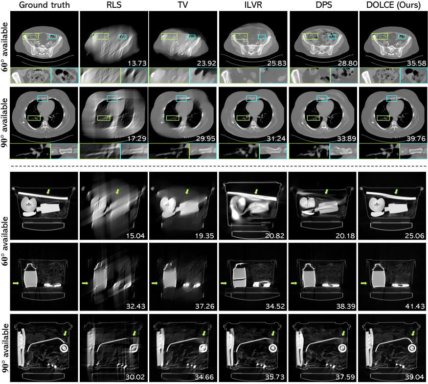
Figure 3: Visual evaluation of limited angle tomographic reconstruction in body CT scan (top) and checked-in luggage (bottom), where the input measurements are captured respectively from an angular coverage of 60^∘ and 90^∘, respectively. PSNR (dB) is indicated at bottom for each reconstruction, measured against the ground truth. Note the remarkable accuracy of DOLCE reconstructions that preserve fine image details. See Table 1 and Table 2 for quantitative comparisons with additional baselines. Images are normalized for better visualization.

5 Experiments

5.1 Datasets

Checked-in Luggage Dataset. The luggage dataset is collected using an Imatron electron-beam medical scanner – a device similar to those found in transportation security systems, provided by the DHS ALERT Center of Excellence at Northeastern University [57] for the development and testing of Automatic Threat Recognition (ATR) systems. The dataset is comprised of $190$ bags, with roughly $300$ slices per bag on an average. In total, the dataset consists of $50$K full view sinograms along with their corresponding FBP reconstructions. The image matrix is resampled to be $512\times 512$, and correspondingly the sinograms are subsampled to be of size 720×512. This corresponds to views obtained at every $0.25^{\circ}$ uniformly sampled from $180^{\circ}$. We repurpose this dataset for generating CT reconstructions from sinograms. We split the bags into a training set of $165$ bags and a test set with the rest, corresponding to about $40$K for training and $10$K for testing. The bags contain a variety of everyday objects, including clothes, food, electronics etc., that are arranged in random configurations.

Metric	PSNR $\,\uparrow$			SSIM $\,\uparrow$
Angle	60∘	90∘	120∘	60∘	90∘	120∘
FBP	15.17	17.51	21.20	0.464	0.540	0.601
RLS	22.75	26.26	30.47	0.698	0.832	0.887
TV [5]	25.60	30.27	36.33	0.791	0.907	0.956
U-Net [40]	26.86	31.31	38.61	0.852	0.932	0.966
DPIR [90]	26.22	31.25	37.60	0.849	0.930	0.951
ILVR [12]	28.63	33.34	37.68	0.861	0.931	0.955
DPS [13]	28.97	33.45	37.92	0.897	0.937	0.959
DOLCE
DOLCE-SA

Table 1: Average PSNR and SSIM results for several methods on human body CT dataset.  and  for each metric are color-coded.

Body CT Scan Datasets. We additionally use Kidney CT scans of 210 patients from the publicly available dataset 2019 Kidney and Kidney Tumor Segmentation Challenge (C4KC-KiTS) [30]. The collection contains 406 scans, where each patient has 1-3 scans. Each 3D scan consists of about $92\sim 812$ 2D slices covering a range of anatomical regions from chest to pelvis, resulted in about $70$K slices in total. We choose $60$K 2D slices of size $512\times 512$ corresponding to 190 patients to train the models. The test images correspond to $10$K slices randomly selected from the remaining patients.

5.2 Training details and parameters

We train and evaluate the models with Pytorch using Tesla V100 GPUs with 16GB memory. To show the effectiveness of our conditional diffusion model, we train a single DOLCE model on the luggage and body CT dataset jointly, by minimizing the loss in Eq. (7). We rescale each dataset globally to make them have the same intensity range, but we do not perform any normalization on those images. As baselines for comparison, we also train individual models on luggage and body CT dataset. For both two datasets, FBP and RLS reconstructions are obtained using publicly available CT reconstruction tools such as LTT [9] and TomoPy [28]. During training, we randomly select FBP or RLS reconstructed using $\theta_{\text{max}}\in\{60^{\circ},90^{\circ},120^{\circ}\}$ as the conditional input, so that the models can handle multiple scenarios. The FBP or RLS is normalized to intensity range of $[0,1]$ for better performance and stable training. We also train two unconditional diffusion models on each dataset and one on the joint dataset as additional baselines. Due to GPU memory constraints, we train all diffusion models in half precision (float16) with a batch-size of $256$. We use the Adam optimizer with a fixed learning rate of $1.5\times 10^{-4}$ and a dropout rate of $0.2$ for each model. We do not perform any checkpoint selection on our models and simply select the latest checkpoint. It takes about two days to obtain a DOLCE model.

5.3 Quantitative and Qualitative Results

Table 1 and Table 2 show average PSNR and SSIM [79] results of several methods for 150 randomly chosen slices from each test set, respectively. The compared methods include FBP, RLS, TV [5], U-Net [40], CTNet [2], DPIR [90], ILVR [12], and DPS [13]. Note that CTNet is a method specifically designed for luggage dataset to reconstruct directly from sinograms. We observed that making CTNet perform well on other datasets requires dedicated fine-tuning so we omit its results on medical dataset for fair comparison. U-Net corresponds to our own implementation of the architecture used in the FBPConvNet [40], and we use the same RLS reconstruction instead of FBP to train the U-Net models. DPIR refers to an iterative deterministic method that uses deep Gaussian denoiser as prior for solving various imaging inverse problems. The denoisers used in DPIR are retrained on our CT datasets. ILVR and DPS are two sampling algorithms that use unconditionally trained diffusion models for solving inverse problems. It is worth noting that to the best of our knowledge there is no existing work that uses diffusion models for LACT reconstruction. We run a grid search over the noise schedule and data-consistency hyper-parameters for both ILVR and DPS, and we observe that both ILVR and DPS perform better in terms of PSNR/SSIM when using models trained separately on each dataset. Accordingly, we report the results that have the best PSNR (dB) values. From Table 1 and Table 2, it is evident that DOLCE is significantly better than existing approaches and significantly outperforms recent methods using unconditionally trained diffusion models.

Metric	PSNR $\,\uparrow$			SSIM $\,\uparrow$
Angle	60∘	90∘	120∘	60∘	90∘	120∘
FBP	25.70	27.87	31.75	0.673	0.694	0.739
RLS	27.45	30.69	34.91	0.756	0.852	0.909
TV [5]	29.13	33.01	39.06	0.811	0.902	0.963
CTNet [2]	29.72	33.39	37.95	0.824	0.895	0.952
U-Net [40]	29.47	33.45	39.22	0.851	0.910	0.972
DPIR [90]	30.40	34.35	38.92	0.845	0.916	0.970
ILVR [12]	29.64	33.06	38.97	0.846	0.911	0.968
DPS [13]	30.96	34.84	38.75	0.885	0.923	0.968
DOLCE
DOLCE-SA

Table 2: Average PSNR and SSIM results comparing test slices with the ground truth from checked-in luggage dataset.

Visual Evaluation. We compare the visual results of DOLCE to RLS, TV, ILVR, and DPS for $\theta_{\text{max}}\in\{60^{\circ},90^{\circ}\}$ in Fig. 3. In general, we observe that RLS is dominated by the artifacts due to missing angles, while TV reduces those artifacts, but blurs the fine structures by producing cartoon-like features. Although ILVR and DPS show better reconstruction with sharper edges than TV, DOLCE produces more accurate reconstructions with fine details. This highlights the SOTA performance of DOLCE using our conditionally trained denoising diffusion model.

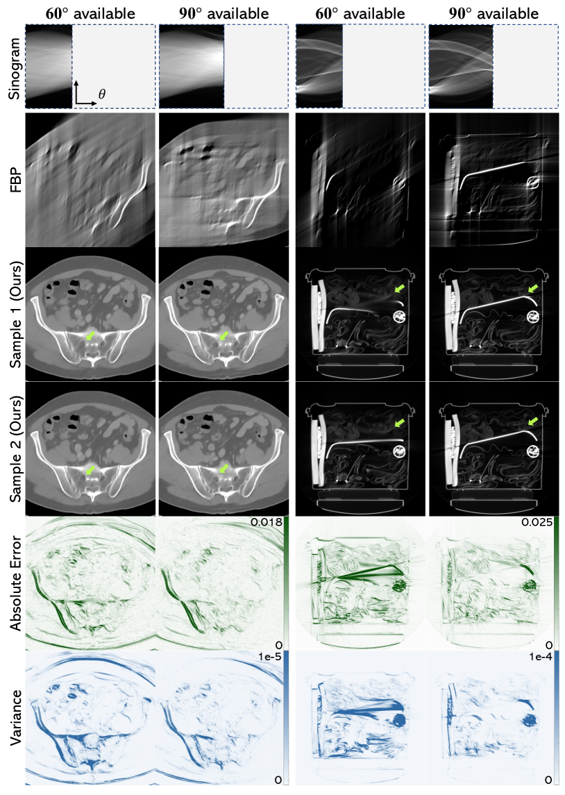
Figure 4: Visual results on two different CT images. The error to the ground truth is computed using the conditional mean $\mathbb{E}[{\bm{x}}|{\bm{y}}]$, and the variance corresponds to per-pixel standard deviation. It is evident that the ill-posed nature of the reconstruction task has a direct impact on the diversity of the generated samples, and the variances are highly correlated with the reconstruction errors.

Angle	Dataset	Lug.	Med.	Lug.+Med.
60∘	Lug.	33.59 / 0.935	26.78 / 0.701	33.98 / 0.935
	Med.	22.56 / 0.726	34.95 / 0.949	35.15 / 0.945
90∘	Lug.	39.19 / 0.966	31.36 / 0.853	39.28 / 0.967
	Med.	29.96 / 0.732	39.28 / 0.969	39.27 / 0.963
120∘	Lug.	45.43 / 0.988	34.71 / 0.933	45.18 / 0.987
	Med.	33.97 / 0.927	43.05 / 0.976	42.52 / 0.974

Table 3: Average PSNR/SSIM results of DOLCE on luggage and medical images, where DOLCE uses two models separately trained on luggage and medical and one trained on the combined dataset.

5.4 Ablation Studies

Capacity for Multiple Data Distributions. We extract additional 150 slices randomly selected from luggage and body CT datasets, respectively, in order to evaluate the effectiveness of our DOLCE using model jointly trained on two distinct datasets (denoted as  “Lug.+Med.”) versus models trained separately. The average PSNR/SSIM values for different limited angles are presented in Table 3. We find that DOLCE is remarkably consistent in matching the performance of the individually trained models across both domains, which highlights the potential of using a single diffusion-based CT reconstruction model to work effectively across a variety of applications.

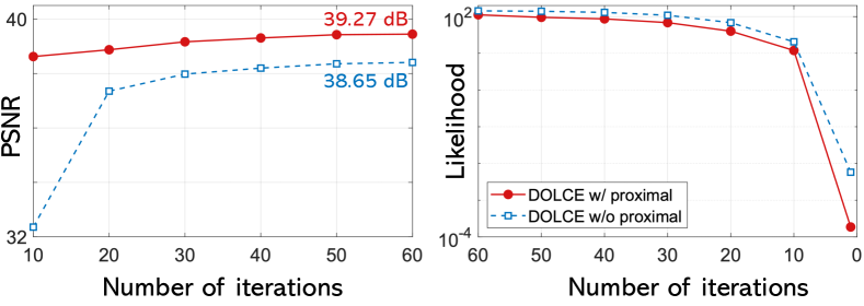
Figure 5: Comparison of average PSNR (left) and likelihood (right) of DOLCE w/ and w/o data-consistency mapping in Eq. (10) on medical CT dataset with $\theta_{\textbf{max}}=$90^∘. Both methods use re-scheduling strategy of IDDPM [56] starting from $K=10$. The likelihood is plotted using $K=60$. Note the improved reconstruction quality by imposing data-consistency during inference.

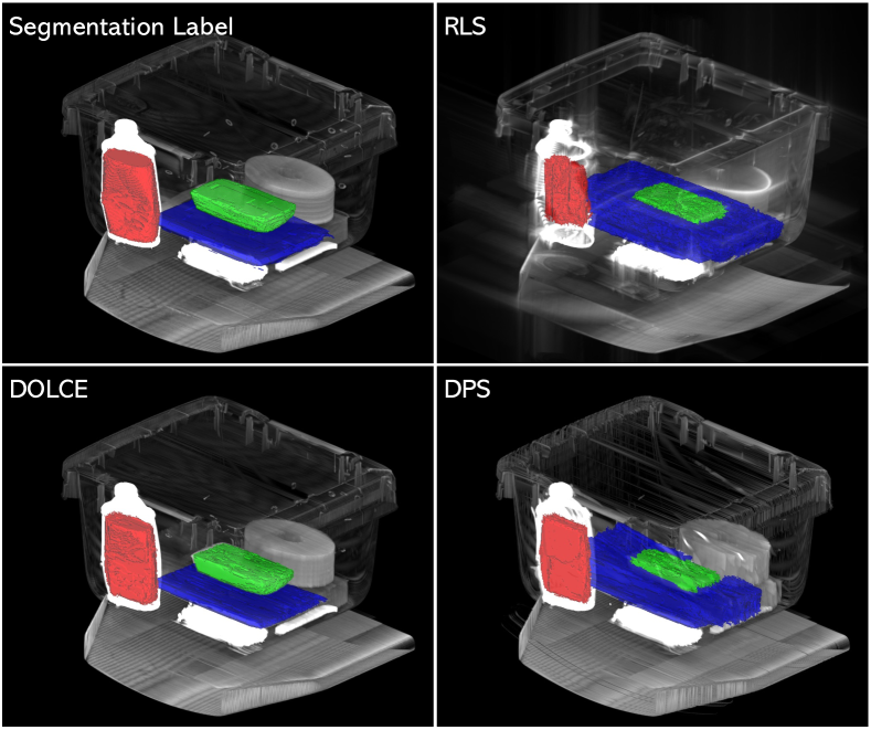
Figure 6: We use a region growing 3D segmentation in all cases and the resulting segmentations are highlighted in color, against a 3D rendering of the reconstructed 2D slices using $\theta_{\text{max}}=$90^∘. Note that our method performs very similar to ground truth in determining the object boundaries compared to RLS and DPS.

Uncertainty Quantification. Fig. 4 shows that DOLCE is able to quantify uncertainty by estimating the variances directly. Since a well-calibrated model indicates larger variance in areas of larger absolute error, variance can be used as a proxy for reconstruction error in the absence of ground truth. It is evident in Fig 4, that the variance images are highly correlated to the absolute error images, reflecting higher uncertainty in the corresponding regions. As expected, we also observe that the level of detail produced by our method is adaptive to the ill-posed nature of the reconstruction task, since more ill-posed input generally leads to higher variance in the resulting samples.

Incorporation of Data-Consistency. Visualizing the trend of PSNR in Fig. 5 (left), we see that the quality of the image improves as we use more number of iterations and remains steady after $K=50$. More importantly, DOLCE using the data-consistency provided in Eq. (10) boosts the reconstruction quality with less sampling steps. Additionally, both DOLCE w/ and w/o proximal mapping are reducing the likelihood during inference as illustrated in Fig. 5 (right), whereas enforcing proximal mapping leads to a lower likelihood as expected, which highlights the potential of enforcing data-consistency within sampling.

5.5 3D Segmentation from CT Reconstructions

Since CT images are primarily used to study 3D objects, we evaluate the quality of the DOLCE reconstructions in 3D segmentation to demonstrate its usefulness in practice. To this end, we use the popular region-growing based segmentation proposed in [83] to identify high intensity objects in the bags from their reconstructions with limited angular range. We show in Fig. 6 an example of a bag (from the test set) with 274 image slices that has been rendered in 3D using the 2D slices reconstructed with the proposed DOLCE. We compare the segmentations obtained using our method to the segmentation labels as reference, and those obtained using RLS and DPS, respectively. Specifically, both RLS and DPS preserves 3D edges poorly resulting in spurious segments, whereas our DOLCE reconstruction is significantly better, resembling the ground truth. Additional segmentation results can be found in the supplementary material.

6 Conclusion

We consider the recovery of high-quality images from the LACT data in the settings where the viewing angles can be as small as 60^∘. Building on the recent work on conditional diffusion models, we present the first model-based probabilistic diffusion framework for LACT called DOLCE. Our framework enables the recovery of high-quality CT images that preserve the geometric structure and sharp edges by using an image prior in the form of a diffusion model conditioned on the transformed limited-angle sinograms. DOLCE can use FBP or RLS images as the conditional input to its diffusion model. During inference, DOLCE enforces the forward model using the data-consistency update implemented as a proximal mapping. As a result, DOLCE imposes both forward-model and prior constraints on the solution. Extensive experimental results demonstrate the SOTA performance of DOLCE on widely different data distributions, such as images of human body and of checked-in luggage, thus enabling highly generalizable LACT reconstruction networks for the first time. Additionally, we show how the diverse realizations produced by DOLCE from a given sinogram can enable meaningful uncertainty quantification. In summary, our work presents a new SOTA method for LACT that enables systematic uncertainty characterization, thus opening a new exciting avenue for future research on diffusion models for severely ill-posed imaging problems such as LACT.

Supplementary Material

Appendix A CT Reconstruction Formulation

In our experiments, the object to be imaged is placed in between a source of parallel beam x-rays and a planar detector array. The x-rays get attenuated as they propagate through the object and the intensity of attenuated x-rays exiting the object is measured by the detector. To perform tomographic imaging, the object is rotated along an axis and repeatedly imaged at regular angular intervals of rotation. Assume that the object is stationary in the Cartesian coordinate system represented by the axes $(x,y,z)$, at each rotation angle $\theta$ of the object, we are interested in reconstructing 2D slice images, denoted as $\rho(x,y,z)$ of object linear attenuation coefficient (LAC) values along the propagation path. The projection at a distance of $r$ on the detector is given by

$$S_{\theta}(r,z)=\int\int\rho(x,y,z)\delta(x\cos(\theta)+y\sin(\theta)-r)\,dxdy,$$ (11)

where $\delta$ is the indicator function and $S_{\theta}(r,z)$ is known as sinogram. Note that equation (LABEL:eq:radon) is separable in the $z$ coordinate. Hence, the projection relation is essentially a 2D function in the $x-y$ plane that is repeatedly applied along the $z$-axis. The reconstruction of $\rho(x,y,z)$ from incomplete sinogram can be formulated as image inverse problem described in the main paper (See [41, 95] for more references).

FBP Reconstruction Filtered back-projection (FBP) is an analytic algorithm for reconstructing the sample $\rho(x,y,z)$ for the projections $S_{\theta}(r,z)$ at all the rotation angles $\theta$. In FBP, we first compute the filtered projection measurement of each slice $\widehat{S}_{\theta}(r)=\int{\mathcal{F}}[S_{\theta}](\omega)|\omega|e^{j2\pi\omega r}d\omega$, where ${\mathcal{F}}$ denotes the Fourier transform and $|\omega|$ is the frequency response of the filter. The filtered back projection reconstruction is then given by [41]

$$f_{\text{FBP}}(x,y)=\int_{0}^{\pi}\widehat{S}_{\theta}(x\cos(\theta)+y\sin(\theta))d\theta.$$ (12)

According to equation (LABEL:eq:fbp), we know that a filtered version of $S_{\theta}$ is smeared back on the $x-y$ plane along the direction ($\pi/2-\theta$). The FBP reconstruction thus consists of the cumulative sum of the smeared contributions from all the projections ranging in $0<\theta<\pi$.

LACT Reconstruction Artifacts by FBP. If the projections are acquired over a limited angular range, then the integration in (LABEL:eq:fbp) will be incomplete in the angular space. Since each projection $S_{\theta}(r)$ contains the cumulative sum of the LAC values at a rotation angle of $\theta$, it also contains information about the edges that are oriented along the angular direction ($\pi/2-\theta$) as shown in Fig. 7. Now, suppose data acquisition starts at $\theta=\text{0}$ and stops at an angle of $\theta=\theta_{\text{max}}<\pi$. Then, the edge information contained in the projections at the angles $\theta\in[\theta_{\text{max}},\pi]$ will be missing in the final reconstruction. This is the reason behind the edge blur in the FBP reconstructions shown in this paper.

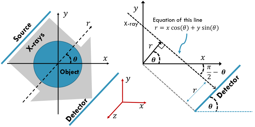
Figure 7: Implementation of x-ray CT. An object is rotated along an axis and exposed to a parallel beam of x-rays. The intensity of attenuated x-rays exiting the object is measured by the detector at regular angular intervals. The projection at an angle of $\theta$ measured at a distance of $r$ on the detector is the line integral of LAC values along the line perpendicular to the detector.

Appendix B Additional Implementation Details

Metric		PSNR $\,\uparrow$			SSIM $\,\uparrow$
Angle		60∘	90∘	120∘	60∘	90∘	120∘
FBP		14.95	17.28	20.97	0.464	0.543	0.603
RLS		22.72	26.19	30.42	0.699	0.833	0.888
DOLCE (FBP, w/o prox)		33.72	38.00	40.63	0.927	0.945	0.954
DOLCE (FBP, w/ prox)		34.05	38.73	42.00	0.938	0.960	0.972
DOLCE (RLS, w/o prox)		34.91	38.65	41.25	0.936	0.951	0.959
DOLCE (RLS, w/ prox)		35.15	39.27	42.52	0.945	0.963	0.974
DOLCE-SA (FBP, w/o prox)		34.31	38.75	41.49	0.936	0.952	0.961
DOLCE-SA (FBP, w/ prox)		34.58	39.28	42.55	0.943	0.963	0.975
DOLCE-SA (RLS, w/o prox)		35.55	39.31	42.12	0.944	0.954	0.965
DOLCE-SA (RLS, w/ prox)		35.78	39.75	43.11	0.949	0.969	0.977

Table 4: Average PSNR and SSIM results comparing test slices with the ground truth from medical body CT dataset.

Metric		PSNR $\,\uparrow$			SSIM $\,\uparrow$
Angle		60∘	90∘	120∘	60∘	90∘	120∘
FBP		26.08	28.34	32.18	0.668	0.713	0.752
RLS		28.05	31.01	35.61	0.775	0.860	0.914
DOLCE (FBP, w/o prox)		33.13	37.43	42.83	0.928	0.953	0.974
DOLCE (FBP, w/ prox)		33.44	38.17	44.12	0.928	0.959	0.983
DOLCE (RLS, w/o prox)		33.70	38.64	43.76	0.933	0.959	0.978
DOLCE (RLS, w/ prox)		33.98	39.28	45.18	0.935	0.967	0.987
DOLCE-SA (FBP, w/o prox)		33.85	38.26	43.74	0.932	0.959	0.978
DOLCE-SA (FBP, w/ prox)		34.11	38.91	44.87	0.931	0.963	0.985
DOLCE-SA (RLS, w/o prox)		34.41	39.40	44.52	0.941	0.966	0.981
DOLCE-SA (RLS, w/ prox)		34.68	39.88	45.68	0.941	0.971	0.988

Table 5: Average PSNR and SSIM results comparing test slices with the ground truth from checked-in luggage dataset.

CTNet [2] is an end-to-end DL method, designed to predict the invisible sinogram data by incorporating a GAN into the neural network architecture. Note that the original CTNet was developed on $128\times 128$ images. To make it work on $512\times 512$ images, given the pre-trained CTNet on $128\times 128$ images, we additionally train a super-resolution diffusion model presented in [63] to super-resolve the low-resolution outputs of CTNet to the same $512\times 512$ dimension as other methods.

DPIR [90] refers to the SOTA PnP methods using deep denoiser as prior for solving various ill-posed image inverse problems. We modify the publicly available implementation to train the deep denoiser  on each dataset separately and follow the similar implementation settings  at inference. Since our CT images are naturally in smaller intensity range, we train the DPIR denoiser for the AWGN removal within noise level of $\sigma\in[0,5]$.

ILVR [12] and DPS [13] refer to recently developed conditioning methods based on unconditionally trained DDPM for solving versatile ill-posed inverse problems. We modify the publicly available implementation of ILVR  and DPS  in order to incorporate our LACT forward-model. We use the similar grid search as DOLCE for fine-tuning the hyper-parameters within ILVR and DPS, respectively.

We train all the diffusion models used in this paper, modified based on the publicly available PyTorch implementation . To indicate the high quality of our pre-trained diffusion models used within ILVR and DPS, we present the random samples from our two unconditionally trained denoising diffusion $512\times 512$ models in Fig. 8 for luggage and medical dataset, respectively.

Appendix C Additional Numerical and Visual Results

Metric		PSNR $\,\uparrow$			SSIM $\,\uparrow$
Angle		45∘	50∘	55∘	45∘	50∘	55∘
FBP		14.49	14.65	14.83	0.321	0.397	0.441
RLS		19.01	19.98	20.95	0.559	0.596	0.632
ILVR [12]		23.85	24.94	26.75	0.815	0.839	0.872
DPS [13]		24.50	25.84	26.71	0.833	0.848	0.870
DOLCE		24.97	27.47	31.02	0.838	0.884	0.934
DOLCE-SA		25.68	27.88	31.51	0.841	0.889	0.939

Table 6: Average PSNR and SSIM results for several methods on body CT dataset. Best values for each metric are highlighted.

Metric		PSNR $\,\uparrow$			SSIM $\,\uparrow$
Angle		45∘	50∘	55∘	45∘	50∘	55∘
FBP		24.59	24.77	25.64	0.653	0.658	0.661
RLS		26.62	26.95	27.31	0.723	0.748	0.758
ILVR [12]		28.99	29.15	29.85	0.856	0.867	0.871
DPS [13]		29.42	29.85	30.40	0.862	0.871	0.878
DOLCE		30.46	31.45	32.39	0.884	0.899	0.921
DOLCE-SA		30.98	31.79	32.98	0.890	0.906	0.925

Table 7: Average PSNR and SSIM results on luggage dataset.

Comparison of RLS and FBP as Conditional Input. In Table 4 and Table 5, we present additional numerical evaluations for FBP and RLS as conditional input of our DOLCE models cross various angular ranges (e.g., $\theta_{\text{max}}\in\{60^{\circ},90^{\circ},120^{\circ}\}$). We use the same random selected 300 images from test luggage and medical dataset as in the main paper, respectively. While DOLCE using FBP as conditional input provides substantial improvements, using RLS input further boost the overall performance.

Incorporation of Data-Consistency. We also report additional numerical validations on the incorporation of forward-model at inference stage in Table 4 and Table 5. We observer that DOLCE using the data-consistency provided by the proximal-mapping produces better quality reconstruction samples, which highlights the potential of enforcing forward-model within sampling step.

Behavior of DOLCE to Model Mismatch. In Table 6 and Table 7, we demonstrate the behavior of our proposed approach for varying number of views during testing. Specifically, we consider the DOLCE for forward-model mismatch scenarios, where the pre-trained DOLCE models in the main paper are tested for $\theta_{\text{max}}\in\{45^{\circ},50^{\circ},55^{\circ}\}$ limited-angle data. For references, we compare DOLCE and DOLCE-SA (sample average) to FBP, RLS, ILVR, and DPS. We can see that our DOLCE consistently outperforms baseline methods even under model mismatch cases.

Additional Visual Evaluation. In Fig. 9, we compare the visual results of DOLCE on medical CT test images to FBP, U-Net, ILVR, and DPS for $\theta_{\max}=60^{\circ}$. Fig. 10-12 present additional visual comparison for several methods on the luggage dataset. In Fig. 13, we compare DOLCE and DOLCE-SA to DPIR and U-Net on each test dataset, respectively. We also provide  video comparisons of our DOLCE reconstruction results in the supplement material.

More Results for Uncertainty Quantification. Fig. 14-16 shows additional numerical validation that DOLCE is able to quantify uncertainty by estimating the variances directly. Since a well-calibrated model indicates larger variance in areas of larger absolute error, variance can be used as a proxy for reconstruction error in the absence of ground truth.

Appendix D 3D Segmentation Results

We presents additional segmentation results on the reconstruction 2D slices obtained from our DOLCE in Fig 17- 21. The purpose of these experiments are to evaluate how quality affects object segmentation. In specific, we use a popular region growing segmentation similar to the method used in [96], which is a simplified version of the method in [83], with a randomly chosen starting position and a fixed kernel size. The luggage dataset contains segmentation labels of objects of interest, and the evaluation focuses on how well each segmentation extracts the labeled object. We reconstruct all slices of each bag through the proposed method and combine them into a single bag in 3D. Then we run the region growing in 3D at multiple, hand-tuned parameter settings (intensity threshold ranging from $0.0001$ to $0.02$), and reported the results from the best performing setting. This is done as some reconstruction results are in poor quality and sensitive to the threshold. We compare the segmentations obtained using our method to the segmentation labels as reference, and those obtained using full-view ground truth, FBP, TV and DPS, respectively. It is evident to observe that our proposed reconstruction segments the objects of interest very similar to the ground truth images, than compared to using baseline methods for reconstruction.

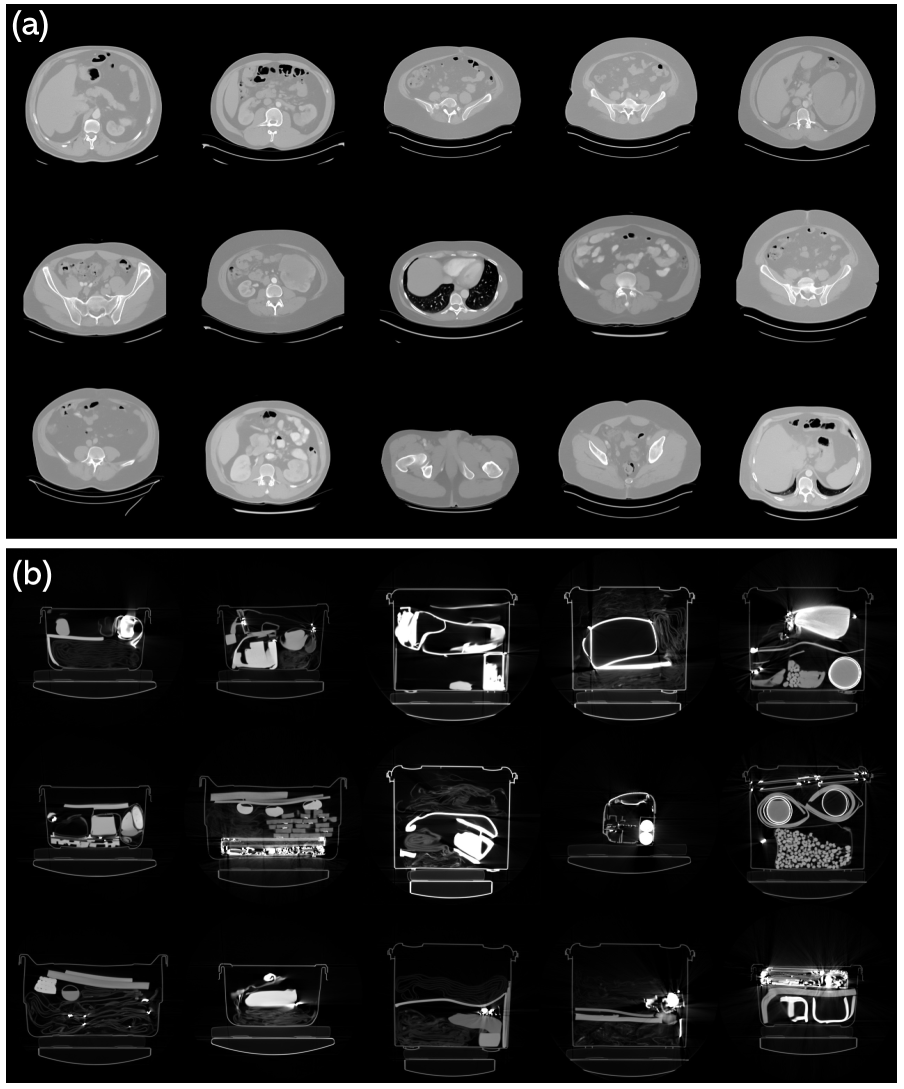
Figure 8: Random samples from our two unconditionally trained denoising diffusion $512\times 512$ models, respectively. (a): diffusion model trained on human body CT images; (b): diffusion model trained on checked-in luggage dataset. These models are used in ILVR [12] and DPS [13] as baseline methods. Images are normalized for better visualization.

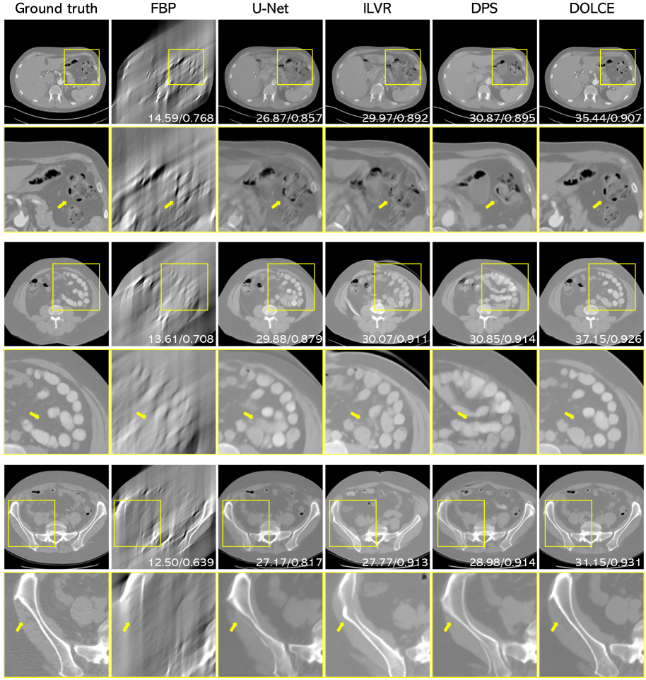
Figure 9: Visual evaluation of limited angle tomographic reconstruction in body CT images, where the input measurements are captured respectively from an angular coverage of 60^∘. Images are normalized for better visualization.

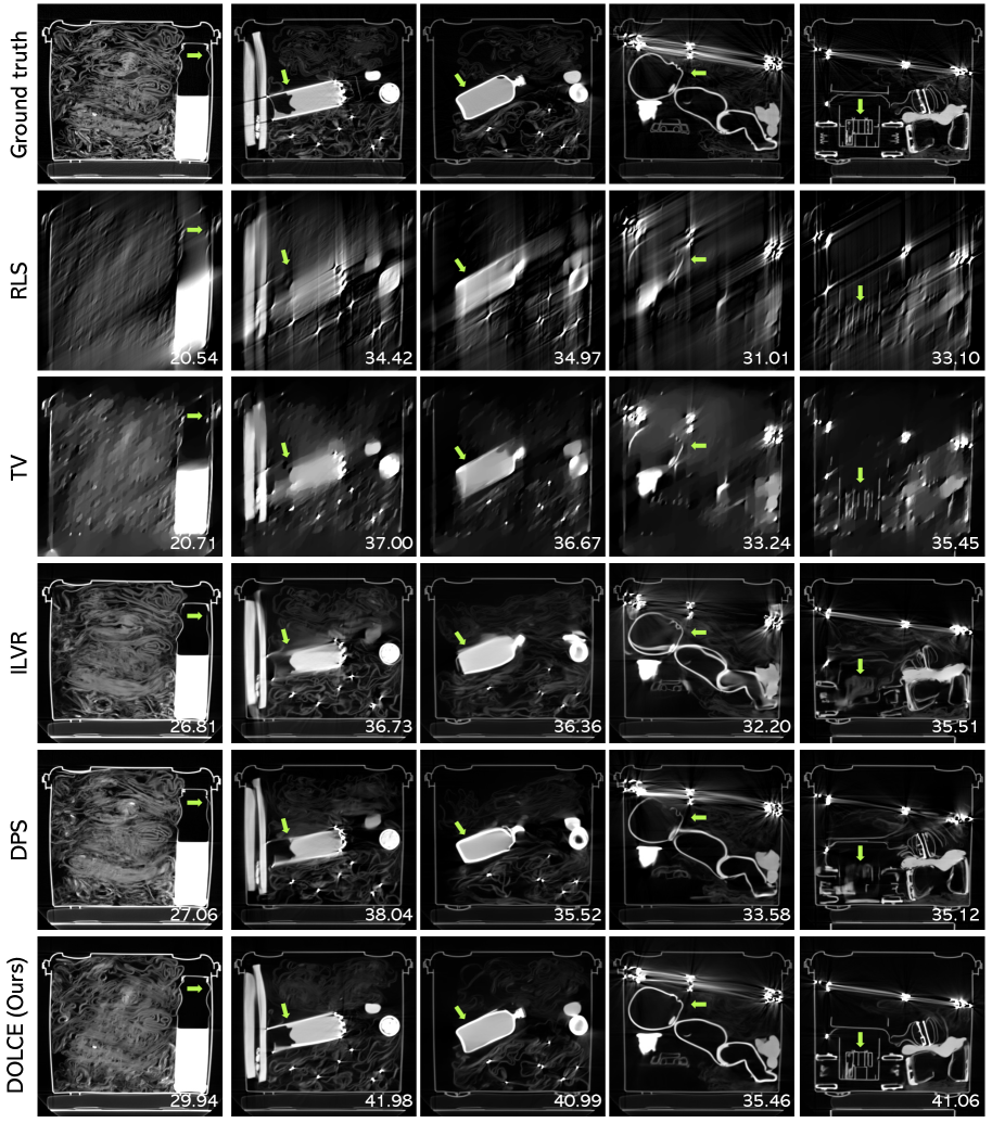
Figure 10: Visual evaluation of limited angle tomographic reconstruction in checked-in luggage, where the input measurements are captured respectively from an angular coverage of 60^∘. Images are normalized for better visualization.

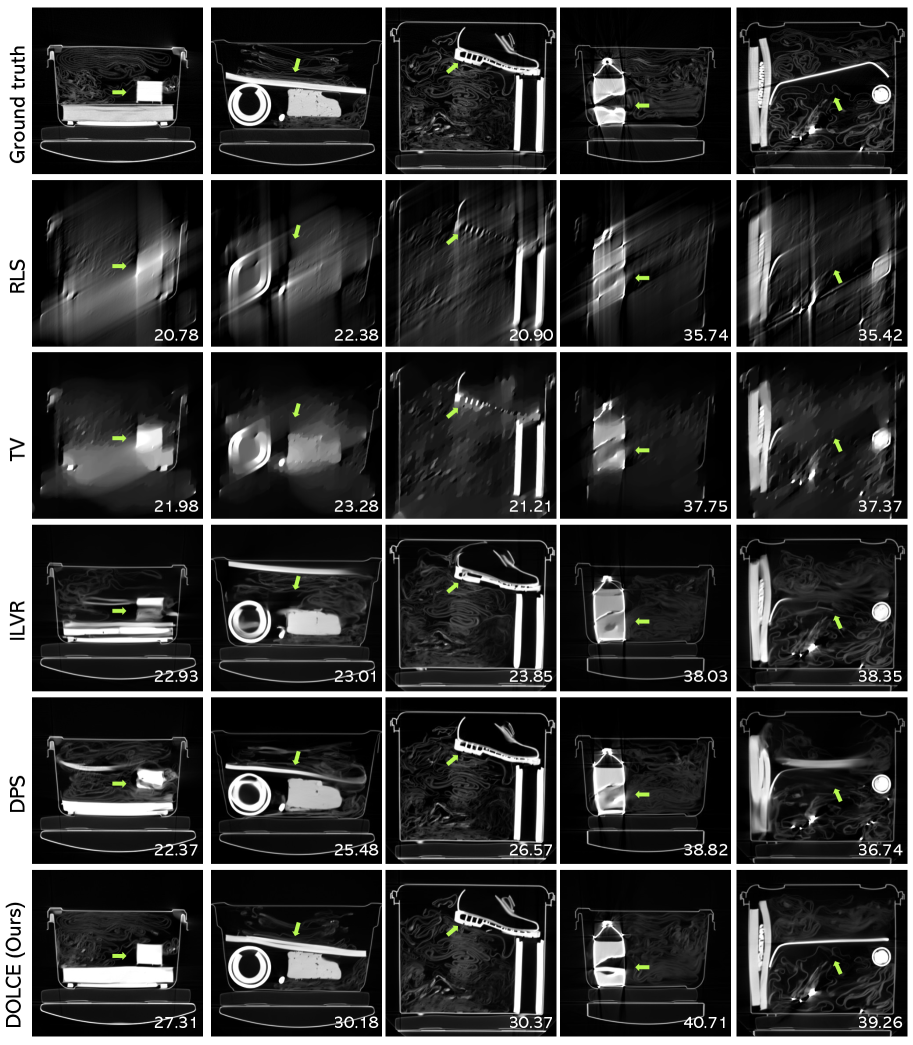
Figure 11: Visual evaluation of limited angle tomographic reconstruction in checked-in luggage, where the input measurements are captured respectively from an angular coverage of 60^∘. Images are normalized for better visualization.

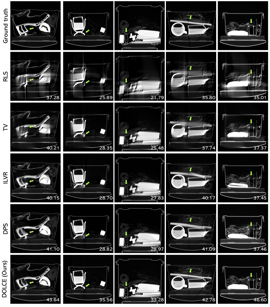
Figure 12: Visual evaluation of limited angle tomographic reconstruction in checked-in luggage, where the input measurements are captured respectively from an angular coverage of 90^∘. Images are normalized for better visualization.

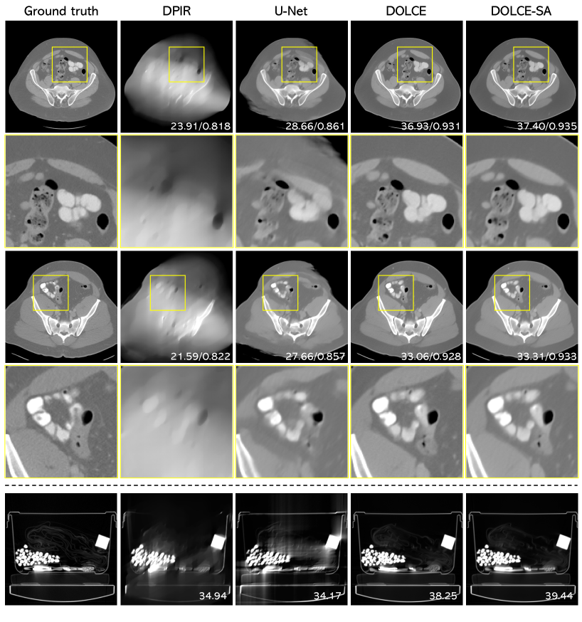
Figure 13: Additional visual evaluation of limited angle tomographic reconstruction in body CT scan (top) and checked-in luggage (bottom), where the input measurements are captured respectively from an angular coverage of 60^∘. Images are normalized for better visualization.

Figure 14: More visual results on body CT images. The error to the ground truth is computed using the conditional mean $\mathbb{E}[{\bm{x}}|{\bm{y}}]$, and the variance corresponds to per-pixel standard deviation. It is evident that the ill-posed nature of the reconstruction task has a direct impact on the diversity of the generated samples, and the variances are highly correlated with the reconstruction errors.

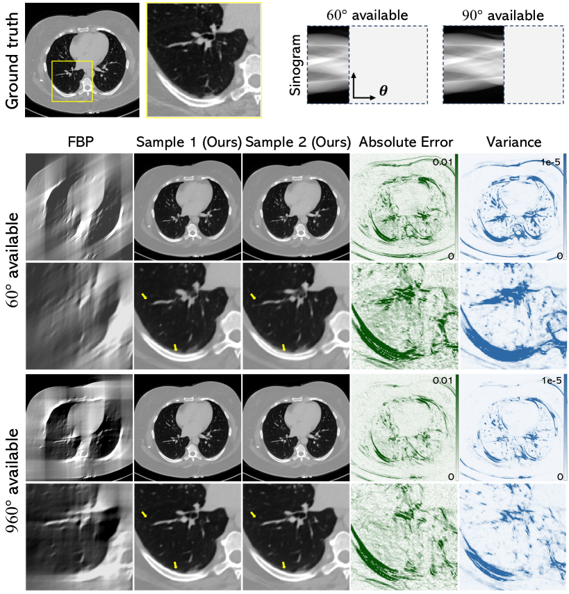
Figure 15: More visual results on body CT images. The error to the ground truth is computed using the conditional mean $\mathbb{E}[{\bm{x}}|{\bm{y}}]$, and the variance corresponds to per-pixel standard deviation. It is evident that the ill-posed nature of the reconstruction task has a direct impact on the diversity of the generated samples, and the variances are highly correlated with the reconstruction errors.

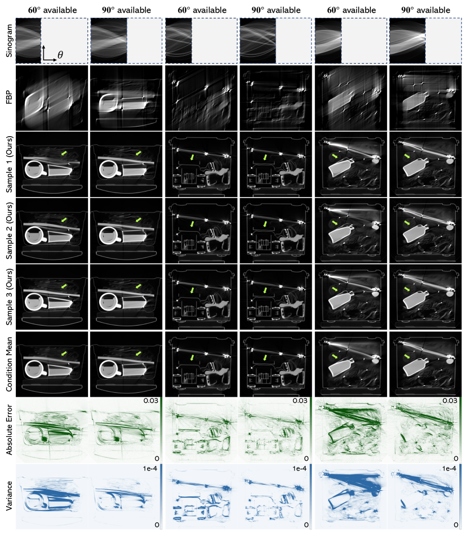
Figure 16: More visual results on luggage images. The error to the ground truth is computed using the conditional mean $\mathbb{E}[{\bm{x}}|{\bm{y}}]$, and the variance corresponds to per-pixel standard deviation. It is evident that the ill-posed nature of the reconstruction task has a direct impact on the diversity of the generated samples, and the variances are highly correlated with the reconstruction errors.

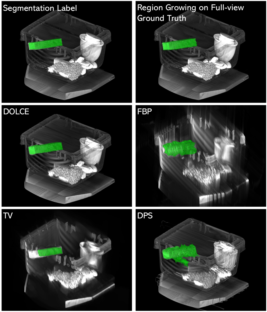
Figure 17: More 3D Segmentation Results on Test Bag 2: We use a region growing 3D segmentation in all cases and the resulting segmentations are highlighted in color, against a 3D rendering of the 274 reconstructed 2D slices using $\theta_{\text{max}}=$60^∘.

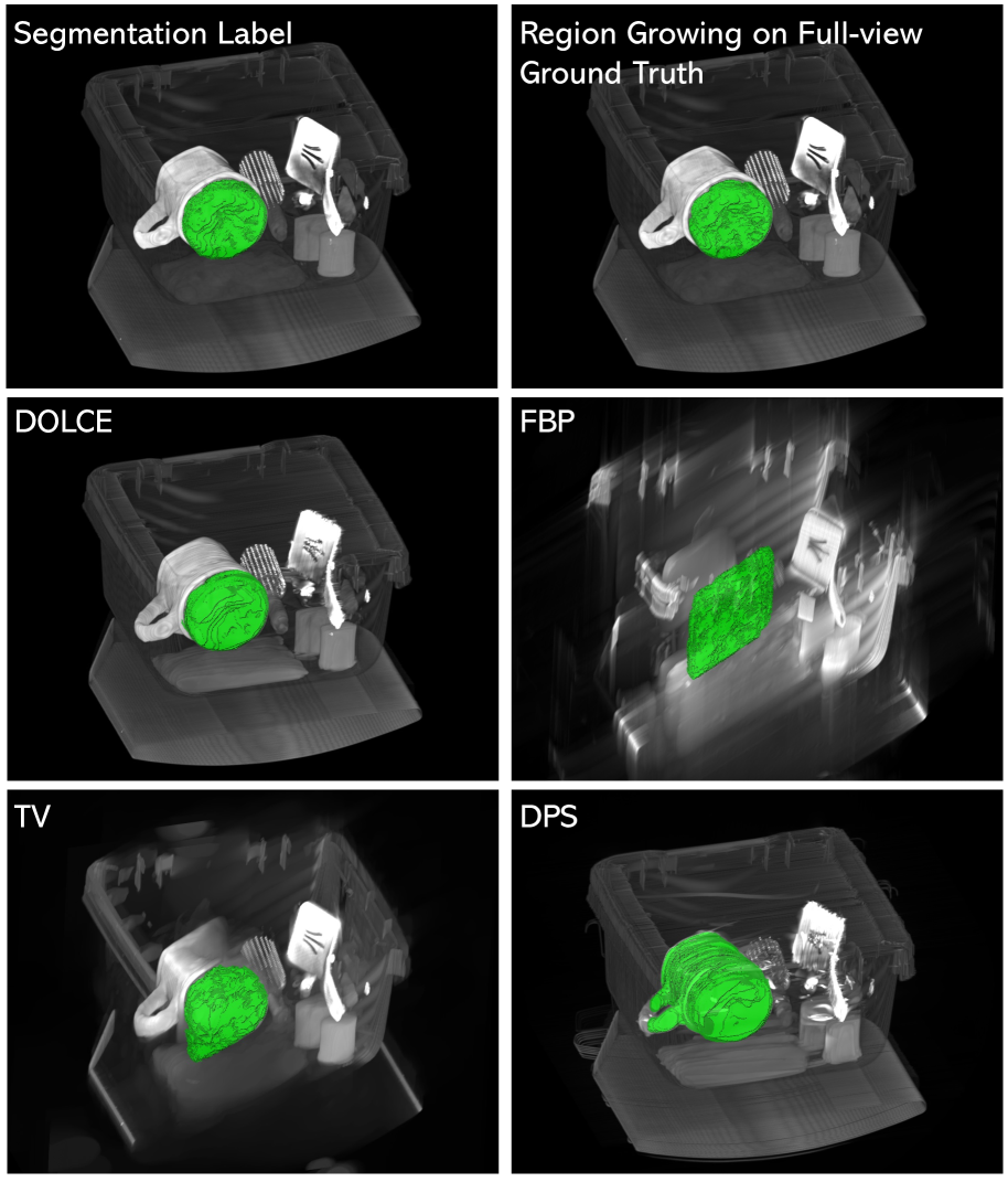
Figure 18: More 3D Segmentation Results on Test Bag 3: We use a region growing 3D segmentation in all cases and the resulting segmentations are highlighted in color, against a 3D rendering of the 274 reconstructed 2D slices using $\theta_{\text{max}}=$60^∘.

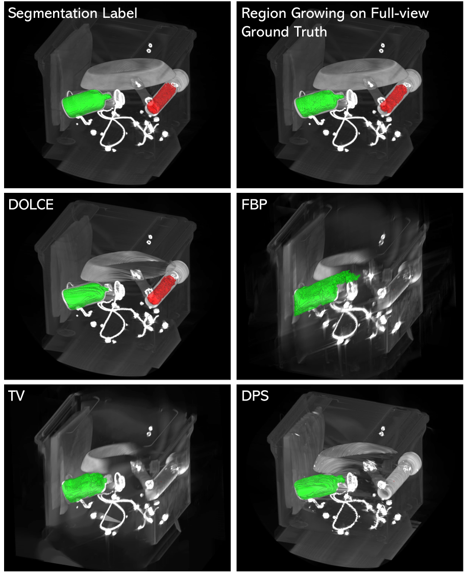
Figure 19: More 3D Segmentation Results on Test Bag 4: We use a region growing 3D segmentation in all cases and the resulting segmentations are highlighted in color, against a 3D rendering of the 268 reconstructed 2D slices using $\theta_{\text{max}}=$60^∘.

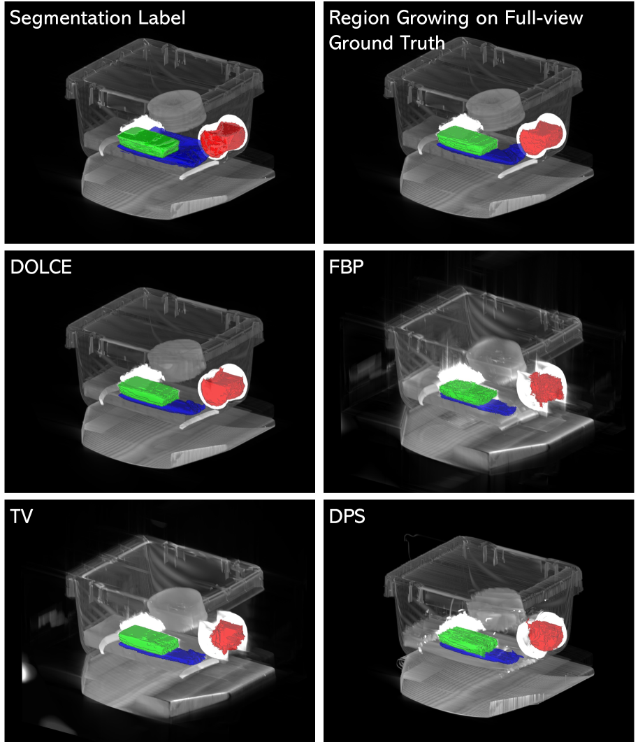
Figure 20: More 3D Segmentation Results on Test Bag 5: We use a region growing 3D segmentation in all cases and the resulting segmentations are highlighted in color, against a 3D rendering of the 274 reconstructed 2D slices using $\theta_{\text{max}}=$90^∘.

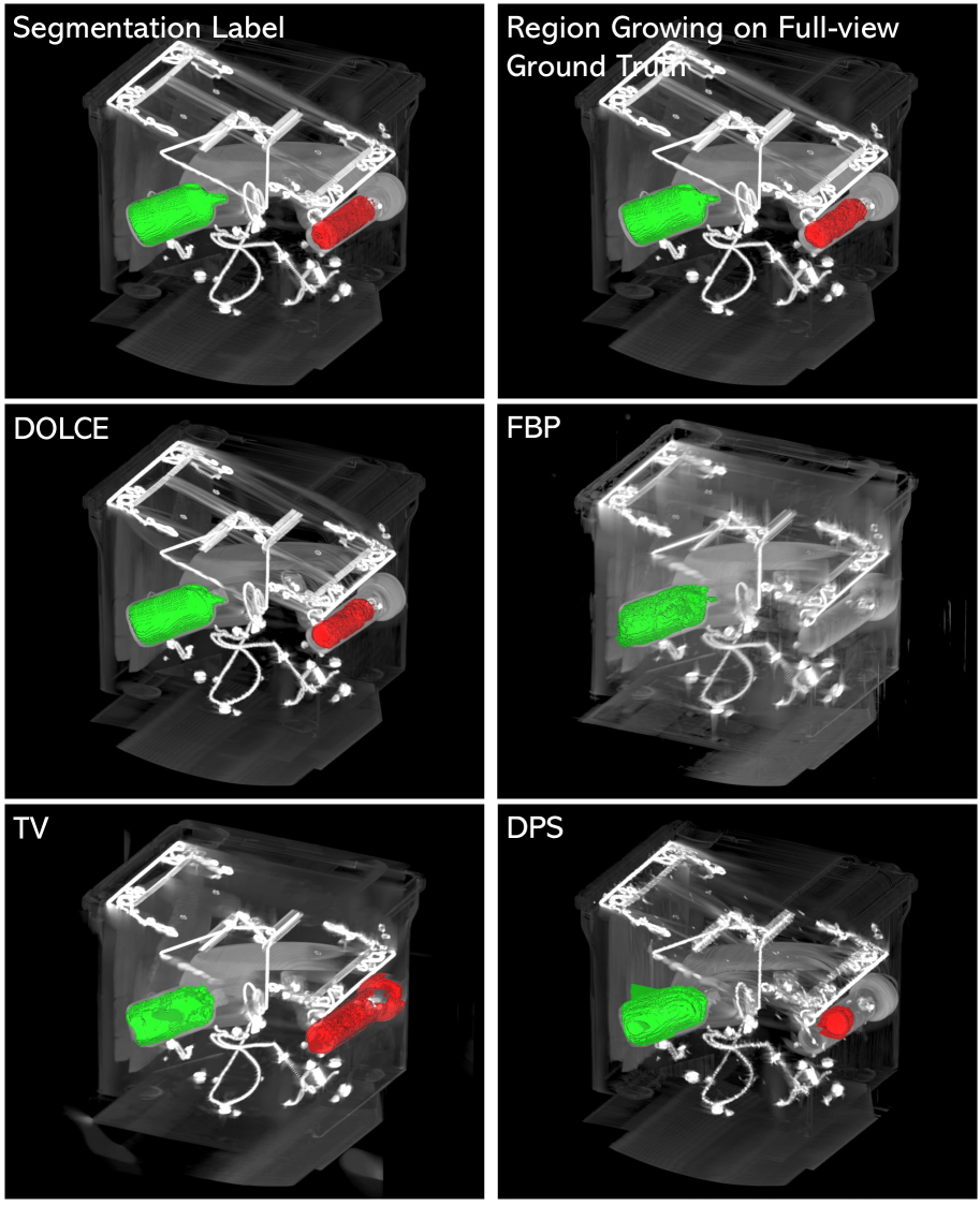
Figure 21: More 3D Segmentation Results on Test Bag 6: We use a region growing 3D segmentation in all cases and the resulting segmentations are highlighted in color, against a 3D rendering of the 268 reconstructed 2D slices using $\theta_{\text{max}}=$90^∘.

References

- [1] J. Adler and O. Öktem. Learned primal-dual reconstruction. IEEE Trans. Med. Imag., 37(6):1322–1332, June 2018.
- [2] R. Anirudh, H. Kim, J. J Thiagarajan, K. A. Mohan, K. Champley, and T. Bremer. Lose the views: Limited angle ct reconstruction via implicit sinogram completion. In Proc. CVPR, pages 6343–6352, 2018.
- [3] G. Bachar, J.H. Siewerdsen, M.J. Daly, D.A. Jaffray, and J.C. Irish. Image quality and localization accuracy in c-arm tomosynthesis-guided head and neck surgery. Medical physics, 34(12):4664–4677, 2007.
- [4] D. O. Baguer, J. Leuschner, and M. Schmidt. Computed tomography reconstruction using deep image prior and learned reconstruction methods. Inverse Problems, 36(9):094004, 2020.
- [5] A. Beck and M. Teboulle. A fast iterative shrinkage-thresholding algorithm for linear inverse problems. SIAM J. Imaging Sciences, 2(1):183–202, 2009.
- [6] C. A. Bouman. Foundations of computational imaging: A model-based approach, 2022.
- [7] A. Brock, J. Donahue, and K. Simonyan. Large scale GAN training for high fidelity natural image synthesis. In Proc. ICLR, 2019.
- [8] T. A. Bubba, M. Galinier, M. Lassas, M. Prato, L. Ratti, and S. Siltanen. Deep neural networks for inverse problems with pseudodifferential operators: An application to limited-angle tomography. 2021.
- [9] K. M. Champley, T. M. Willey, H. Kim, K. Bond, S. M. Glenn, J. A. Smith, J. S. Kallman, W. D. Brown, and et al. Seetho, I. M. Livermore tomography tools: Accurate, fast, and flexible software for tomographic science. NDT & E International, 126:102595, 2022.
- [10] W. Cheng, Y. Wang, H. Li, and Y. Duan. Learned full-sampling reconstruction from incomplete data. IEEE Trans. Comput. Imag, 6:945–957, 2020.
- [11] J. H. Cho and J. A. Fessler. Motion-compensated image reconstruction for cardiac ct with sinogram-based motion estimation. In 2013 IEEE Nuclear Science Symposium and Medical Imaging Conference (2013 NSS/MIC), pages 1–5, 2013.
- [12] J. Choi, S. Kim, Y. Jeong, Y. Gwon, and S. Yoon. Ilvr: Conditioning method for denoising diffusion probabilistic models. In Proc. ICCV, pages 14347–14356, 2021.
- [13] H. Chung, J. Kim, M. T. Mccann, M. L. Klasky, and J. C. Ye. Diffusion posterior sampling for general noisy inverse problems. arXiv preprint arXiv:2209.14687, 2022.
- [14] H. Chung, B. Sim, D. Ryu, and J. C. Ye. Improving diffusion models for inverse problems using manifold constraints. arXiv preprint arXiv:2206.00941, 2022.
- [15] H. Chung, B. Sim, and J. C. Ye. Come-closer-diffuse-faster: Accelerating conditional diffusion models for inverse problems through stochastic contraction. In Proc. CVPR, pages 12413–12422, 2022.
- [16] H. Chung and J. C. Ye. Score-based diffusion models for accelerated mri. Med. Image Anal., page 102479, 2022.
- [17] A. Danielyan, V. Katkovnik, and K. Egiazarian. BM3D frames and variational image deblurring. IEEE Trans. Image Process., 21(4):1715–1728, Apr. 2012.
- [18] L. De Chiffre, S. Carmignato, J.-P. Kruth, R. Schmitt, and A. Weckenmann. Industrial applications of computed tomography. CIRP annals, 63(2):655–677, 2014.
- [19] P. Dhariwal and A. Nichol. Diffusion models beat gans on image synthesis. In Proc. NeurIPS, volume 34, pages 8780–8794, 2021.
- [20] M. Elad and M. Aharon. Image denoising via sparse and redundant representations over learned dictionaries. IEEE Trans. Image Process., 15(12):3736–3745, Dec. 2006.
- [21] M. A. T. Figueiredo and R. D. Nowak. Wavelet-based image estimation: An empirical Bayes approach using Jeffreys’ noninformative prior. IEEE Trans. Image Process., 10(9):1322–1331, Sep. 2001.
- [22] J. Fu, J. Dong, and F. Zhao. A deep learning reconstruction framework for differential phase-contrast computed tomography with incomplete data. IEEE Trans. Imag. Process., 29:2190–2202, 2019.
- [23] M. Gadelha, R. Wang, and S. Maji. Shape reconstruction using differentiable projections and deep priors. In Proc. ICCV, pages 22–30, 2019.
- [24] Q. Gao, R. Ding, L. Wang, B. Xue, and Y. Duan. Lrip-net: low-resolution image prior based network for limited-angle ct reconstruction. IEEE Trans. Radiat. Plasma Med. Sci., 2022.
- [25] D. Gilton, G. Ongie, and R. Willett. Neumann networks for linear inverse problems in imaging. IEEE Trans. on Comput. Imag., 6:328–343, 2020.
- [26] R. Gordon, R. Bender, and G. T. Herman. Algebraic reconstruction techniques (art) for three-dimensional electron microscopy and x-ray photography. Journal of theoretical Biology, 29(3):471–481, 1970.
- [27] H. Gupta, K. H. Jin, H. Q. Nguyen, M. T. McCann, and M. Unser. CNN-based projected gradient descent for consistent ct image reconstruction. IEEE Trans. Med. Imag., 37(6):1440–1453, Jun. 2018.
- [28] D. Gürsoy, F. De Carlo, X. Xiao, and C. Jacobsen. Tomopy: a framework for the analysis of synchrotron tomographic data. Journal of synchrotron radiation, 21(5):1188–1193, 2014.
- [29] Y. Han and J. C. Ye. Framing U-Net via deep convolutional framelets: Application to sparse-view CT. IEEE Trans. Med. Imag., 37(6):1418–1429, 2018.
- [30] N. Heller, N. Sathianathen, A. Kalapara, E. Walczak, K. Moore, H. Kaluzniak, J. Rosenberg, P. Blake, Z. Rengel, M. Oestreich, J. Dean, M. Tradewell, A. Shah, R. Tejpaul, Z. Edgerton, M. Peterson, S. Raza, S. Regmi, N. Papanikolopoulos, and C. Weight. Data from c4kc-kits [data set]. The Cancer Imaging Archive, 2019.
- [31] Ma. R. Hestenes and E. Stiefel. Methods of conjugate gradients for solving linear systems. J. Res. Natl. Bur. Stand., 49(6):409, 1952.
- [32] J. Ho, A. Jain, and P. Abbeel. Denoising diffusion probabilistic models. In Proc. NeurIPS, volume 33, pages 6840–6851, 2020.
- [33] J. Ho and T. Salimans. Classifier-free diffusion guidance. In NeurIPS 2021 Workshop on Deep Generative Models and Downstream Applications, 2021.
- [34] D. Hu, Y. Zhang, J. Liu, C. Du, J. Zhang, S. Luo, G. Quan, Q. Liu, Y. Chen, and L. Luo. Special: single-shot projection error correction integrated adversarial learning for limited-angle ct. IEEE Trans. on Comput. Imag., 7:734–746, 2021.
- [35] D. Hu, Y. Zhang, J. Liu, S. Luo, and Y. Chen. Dior: deep iterative optimization-based residual-learning for limited-angle ct reconstruction. IEEE Trans. on Med. Imag., 41(7):1778–1790, 2022.
- [36] C. Huang, J. H. Lim, and A. C. Courville. A variational perspective on diffusion-based generative models and score matching. In Proc. NeurIPS, volume 34, pages 22863–22876, 2021.
- [37] Y. Huang, X. Huang, O. Taubmann, Y. Xia, V. Haase, J. Hornegger, G. Lauritsch, and A. Maier. Restoration of missing data in limited angle tomography based on helgason–ludwig consistency conditions. Biomed. Phys. Eng. Express., 3(3):035015, 2017.
- [38] Y. Huang, O. Taubmann, X. Huang, V. Haase, G. Lauritsch, and A. Maier. Scale-space anisotropic total variation for limited angle tomography. IEEE Trans. Radiat. Plasma Med. Sci., 2(4):307–314, 2018.
- [39] N. Hyvönen, M. Kalke, M. Lassas, H. Setälä, and S. Siltanen. Three-dimensional dental x-ray imaging by combination of panoramic and projection data. Inverse Problems & Imaging, 4(2):257, 2010.
- [40] K. H. Jin, M. T. McCann, E. Froustey, and M. Unser. Deep convolutional neural network for inverse problems in imaging. IEEE Trans. Image Process., 26(9):4509–4522, Sep. 2017.
- [41] A. C. Kak and M. Slaney. Principles of computerized tomographic imaging. SIAM, 2001.
- [42] B. Kawar, M. Elad, S. Ermon, and J. Song. Denoising diffusion restoration models. In Proc. NeurIPS, 2022.
- [43] A. Kendall and Y. Gal. What uncertainties do we need in bayesian deep learning for computer vision? In Proc. NeurIPS, volume 30, 2017.
- [44] D. P. Kingma, T. Salimans, B. Poole, and J. Ho. Variational diffusion models. In Proc. NeurIPS, volume 34, pages 21696–21707, 2021.
- [45] H. Kudo, T. Suzuki, and E. A. Rashed. Image reconstruction for sparse-view ct and interior ct—introduction to compressed sensing and differentiated backprojection. Quant. Imaging. Med. Surg., 3(3):147, 2013.
- [46] Hoyeon Lee, Jongha Lee, and Suengryong Cho. View-interpolation of sparsely sampled sinogram using convolutional neural network. In Medical Imaging 2017: Image Processing, volume 10133, pages 617–624. SPIE, 2017.
- [47] H. Lee, J. Lee, H. Kim, B. Cho, and S. Cho. Deep neural network based sinogram synthesis for sparse-view ct image reconstruction. IEEE Trans. Radiat. Plasma Med. Sciences, 3(2):109–119, 2019.
- [48] J. Liu, Y. Sun, W. Gan, B. Wohlberg, and U. S. Kamilov. Sgd-net: Efficient model-based deep learning with theoretical guarantees. IEEE Trans. Comput. Imag., 7:598–610, 2021.
- [49] J. Liu, X. Xu, W. Gan, S. Shoushtari, and U. S. Kamilov. Online deep equilibrium learning for regularization by denoising. In Proc. NeruIPS, 2022.
- [50] A. Lugmayr, M. Danelljan, A. Romero, F. Yu, R. Timofte, and L. Van Gool. Repaint: Inpainting using denoising diffusion probabilistic models. In Proc. CVPR, pages 11461–11471, 2022.
- [51] S. Majee, T. Balke, C. A.J. Kemp, G. T. Buzzard, and C. A. Bouman. Multi-slice fusion for sparse-view and limited-angle 4d ct reconstruction. IEEE Trans. Comput. Imag., 7:448–462, 2021.
- [52] C. McCollough. TU-FG-207A-04: Overview of the low dose CT grand challenge. Med. Phys, 43(6Part35):3759–3760, 2016.
- [53] C. Metzler, P. Schniter, A. Veeraraghavan, and R. Baraniuk. prDeep: Robust phase retrieval with a flexible deep network. In Proc ICML, pages 3501–3510, Jul. 10–15 2018.
- [54] K. A. Mohan, S. V. Venkatakrishnan, J. W. Gibbs, E. B. Gulsoy, X. Xiao, M. De Graef, P. W. Voorhees, and C. A. Bouman. TIMBIR: A method for time-space reconstruction from interlaced views. IEEE Trans. Comput. Imag., 1(2):96–111, 2015.
- [55] J. J. Moreau. Proximité et dualité dans un espace Hilbertien. Bull. Soc. Math. France, 93:273–299, 1965.
- [56] A. Q. Nichol and P. Dhariwal. Improved denoising diffusion probabilistic models. In Proc. ICML, pages 8162–8171, 2021.
- [57] D. Center of Excellence at Northeastern University. Alert to4 datasets for automated threat recognition. available at http://www.northeastern.edu/alert. 2014.
- [58] E. T. Quinto and O. Öktem. Local tomography in electron microscopy. SIAM Journal on Applied Mathematics, 68(5):1282–1303, 2008.
- [59] Y. Romano, M. Elad, and P. Milanfar. The little engine that could: Regularization by denoising (RED). SIAM J. Imaging Sci., 10(4):1804–1844, 2017.
- [60] O. Ronneberger, P. Fischer, and T. Brox. U-Net: Convolutional networks for biomedical image segmentation. In Proc. Med. Image. Comput. Comput. Assist. Intervent., pages 234–241, 2015.
- [61] D. Rückert, Y. Wang, R. Li, R. Idoughi, and W. Heidrich. Neat: Neural adaptive tomography. arXiv preprint arXiv:2202.02171, 2022.
- [62] C. Saharia, W. Chan, S. Saxena, L. Li, J. Whang, E. Denton, S. K. S. Ghasemipour, B. K. Ayan, S. S. Mahdavi, R. G. Lopes, et al. Photorealistic text-to-image diffusion models with deep language understanding. In Proc. NeurIPS, 2022.
- [63] C. Saharia, J. Ho, W. Chan, T. Salimans, D. J. Fleet, and M. Norouzi. Image super-resolution via iterative refinement. IEEE Trans. Pattern Anal. Mach. Intell., 2022.
- [64] J. Sohl-Dickstein, E. Weiss, N. Maheswaranathan, and S. Ganguli. Deep unsupervised learning using nonequilibrium thermodynamics. In Proc. ICML, pages 2256–2265, 2015.
- [65] Y. Song and S. Ermon. Generative modeling by estimating gradients of the data distribution. In Proc. NeurIPS, volume 32, 2019.
- [66] Y. Song and S. Ermon. Improved techniques for training score-based generative models. In Proc. NeurIPS, volume 33, pages 12438–12448, 2020.
- [67] Y Song, L. Shen, L. Xing, and S. Ermon. Solving inverse problems in medical imaging with score-based generative models. In Proc. ICLR, 2022.
- [68] Y. Song, J. Sohl-Dickstein, D. P. Kingma, A. Kumar, S. Ermon, and B. Poole. Score-based generative modeling through stochastic differential equations. arXiv preprint arXiv:2011.13456, 2020.
- [69] S. Sreehari, S. V. Venkatakrishnan, B. Wohlberg, G. T. Buzzard, L. F. Drummy, J. P. Simmons, and C. A. Bouman. Plug-and-play priors for bright field electron tomography and sparse interpolation. IEEE Trans. Comput. Imaging, 2(4):408–423, Dec. 2016.
- [70] Y. Sun, J. Liu, and U. S. Kamilov. Block coordinate regularization by denoising. In Proc. NeurIPS, Dec. 2019.
- [71] Y. Sun, J. Liu, M. Xie, B. Wohlberg, and U. S. Kamilov. Coil: Coordinate-based internal learning for tomographic imaging. IEEE Trans. Comput. Imag., 7:1400–1412, 2021.
- [72] M. Usman Ghani and W. Clem Karl. Integrating data and image domain deep learning for limited angle tomography using consensus equilibrium. In Proc. ICCV Workshops, pages 0–0, 2019.
- [73] F. Vasconcelos, B. He, N. Singh, and Y. W. Teh. Uncertainr: Uncertainty quantification of end-to-end implicit neural representations for computed tomography. arXiv preprint arXiv:2202.10847, 2022.
- [74] S. V. Venkatakrishnan, C. A. Bouman, and B. Wohlberg. Plug-and-play priors for model based reconstruction. In Proc. IEEE Global Conf. Signal Process. and Inf. Process., pages 945–948, Austin, TX, USA, Dec. 3-5, 2013.
- [75] S. V. Venkatakrishnan, L. F. Drummy, M. A. Jackson, M. De Graef, J. Simmons, and C. A. Bouman. A model based iterative reconstruction algorithm for high angle annular dark field-scanning transmission electron microscope (haadf-stem) tomography. IEEE Trans. Imag. Process., 22(11):4532–4544, 2013.
- [76] S. V. Venkatakrishnan, K. A. Mohan, A. K. Ziabari, and C. A. Bouman. Algorithm-driven advances for scientific ct instruments: from model-based to deep learning-based approaches. IEEE Signal Process. Mag., 39(1):32–43, 2021.
- [77] G. Wang, J. C. Ye, K. Mueller, and J. A. Fessler. Image reconstruction is a new frontier of machine learning. IEEE Trans. Med. Imag., 37(6):1289–1296, 2018.
- [78] G. Wang, H. Yu, and B. De Man. An outlook on x-ray ct research and development. Medical physics, 35(3):1051–1064, 2008.
- [79] Z. Wang, A. C. Bovik, H. R. Sheikh, and E. P. Simoncelli. Image quality assessment: from error visibility to structural similarity. IEEE Trans. Image Process., 13(4):600–612, Apr 2004.
- [80] K. Wei, A. I. Avilés-Rivero, J. Liang, Y. Fu, H. Huang, and C. B. Schönlieb. Tfpnp: Tuning-free plug-and-play proximal algorithms with applications to inverse imaging problems. J. Mach. Learn. Res.(JMLR), 23(16):1–48, 2022.
- [81] K. Wells and D.A. Bradley. A review of x-ray explosives detection techniques for checked baggage. Applied Radiation and Isotopes, 70(8):1729–1746, 2012.
- [82] J. Whang, M. Delbracio, H. Talebi, C. Saharia, A. G. Dimakis, and P. Milanfar. Deblurring via stochastic refinement. In Proc. CVPR, pages 16293–16303, 2022.
- [83] D. F. Wiley, D. Ghosh, and C. Woodhouse. Automatic segmentation of ct scans of checked baggage. In Proceedings of the 2nd International Meeting on Image Formation in X-ray CT, pages 310–313, 2012.
- [84] Q. Wu, R. Feng, H. Wei, J. Yu, and Y. Zhang. Self-supervised coordinate projection network for sparse-view computed tomography. arXiv preprint arXiv:2209.05483, 2022.
- [85] W. Xia, Q. Lyu, and G. Wang. Low-dose ct using denoising diffusion probabilistic model for 20 speedup. arXiv preprint arXiv:2209.15136, 2022.
- [86] Y. Xie and Q. Li. Measurement-conditioned denoising diffusion probabilistic model for under-sampled medical image reconstruction. arXiv preprint arXiv:2203.03623, 2022.
- [87] M. Xu, D. Hu, F. Luo, F. Liu, S. Wang, and W. Wu. Limited-angle x-ray ct reconstruction using image gradient -norm with dictionary learning. IEEE Trans. Radiat. Plasma Med. Sci., 5(1):78–87, 2020.
- [88] J. C. Ye, Y. Han, and E. Cha. Deep convolutional framelets: A general deep learning framework for inverse problems. SIAM J. Imag. Sci., 11(2):991–1048, 2018.
- [89] G. Zang, R. Idoughi, R. Li, P. Wonka, and W. Heidrich. Intratomo: Self-supervised learning-based tomography via sinogram synthesis and prediction. In Proc. ICCV, pages 1960–1970, 2021.
- [90] K. Zhang, Y. Li, W. Zuo, L. Zhang, L. Van Gool, and R. Timofte. Plug-and-play image restoration with deep denoiser prior. IEEE Trans. Patt. Anal. and Machine Intell., pages 1–1, 2021.
- [91] Q. Zhang, Z. Hu, C. Jiang, H. Zheng, Y. Ge, and D. Liang. Artifact removal using a hybrid-domain convolutional neural network for limited-angle computed tomography imaging. Phys. Med. Biol., 65(15):155010, 2020.
- [92] Y. Zhang, T. Lv, R. Ge, Q. Zhao, D. Hu, L. Zhang, J. Liu, Y. Zhang, Q. Liu, W. Zhao, and Y. Chen. Cd-net: Comprehensive domain network with spectral complementary for dect sparse-view reconstruction. IEEE Trans. Comput. Imag., 7:436–447, 2021.
- [93] B. Zhou, X. Chen, S. K. Zhou, J. S. Duncan, and C. Liu. Dudodr-net: Dual-domain data consistent recurrent network for simultaneous sparse view and metal artifact reduction in computed tomography. Medical Image Analysis, 75:102289, 2022.
- [94] B. Zhou, S. K. Zhou, J. S. Duncan, and C. Liu. Limited view tomographic reconstruction using a cascaded residual dense spatial-channel attention network with projection data fidelity layer. IEEE Trans. Med. Imag., 40(7):1792–1804, 2021.
- [95] Radon, J. On the determination of functions from their integral values along certain manifolds. IEEE transactions on medical imaging, 5(4):170–176, 1986.
- [96] Kim, H. and Thiagarajan, J. J. and Bremer, P.T. On the determination of functions from their integral values along certain manifolds. Proc. ICCV, pages 1707-1715, 2015.