Neural Dependencies Emerging from Learning Massive Categories

Abstract

This work presents two astonishing findings on neural networks learned for large-scale image classification. 1) Given a well-trained model, the logits predicted for some category can be directly obtained by linearly combining the predictions of a few other categories, which we call neural dependency. 2) Neural dependencies exist not only within a single model, but even between two independently learned models, regardless of their architectures. Towards a theoretical analysis of such phenomena, we demonstrate that identifying neural dependencies is equivalent to solving the Covariance Lasso (CovLasso) regression problem proposed in this paper. Through investigating the properties of the problem solution, we confirm that neural dependency is guaranteed by a redundant logit covariance matrix, which condition is easily met given massive categories, and that neural dependency is highly sparse, implying that one category correlates to only a few others. We further empirically show the potential of neural dependencies in understanding internal data correlations, generalizing models to unseen categories, and improving model robustness with a dependency-derived regularizer. Code for this work will be made publicly available.

1 Introduction

Despite the tremendous success of deep neural networks in recognizing massive categories of objects [7, 13, 10, 8, 14, 12, 26, 24, 6, 21], how they manage to organize and relate different categories remains less explored. A proper analysis of such a problem is beneficial to understanding the network behavior, which further facilitates a better utilization of this powerful tool.

In this work, we reveal that a deep model tends to make its own way of data exploration, which sometimes contrasts sharply with human consciousness. We reveal some underlying connections between the predictions from a well-learned image classification model, which appears as one category highly depending on a few others. In the example given in Fig. 1a, we can directly replace the logits predicted for “macaw” with a linear combination of the logits for “ostrich”, “bittern”, etc. (without tuning the network parameters) and achieve similar performance. We call this phenomenon as neural dependency, which automatically emerges from learning massive categories. A more surprising finding is that neural dependencies exist not only within a single model, but also between two independently learned models, as shown in Fig. 1b. It is noteworthy that these two models can even have different architectures (e.g., one with convolutional neural network [10] and the other with transformer [8, 14]) and different training strategies.

Towards figuring out what brings neural dependencies and whether they happen accidentally, we make a theoretical investigation and confirm that identifying neural dependencies is equivalent to solving a carefully designed convex optimization—the Covariance Lasso (CovLasso) regression problem proposed in this paper. Such a problem owns a smooth solution path when varying its hyper-parameters [20], which has two appealing properties. First, the solution is guaranteed by a redundant covariance matrix of the category-wise logits. This condition is easily met when the model is trained on a sufficiently large number of categories [9]. Second, the solution admits elegant sparsity. It implies that a category involved in neural dependencies only relates to several instead of numerous other categories.

We further study the potential utilities of neural dependencies, as a support to our theoretical contributions. One straightforward application is to help interpret the internal data correlations, such as what categories are more likely to link to each other (Sec. 3.1). Another application is to investigate how we can generalize a well-learned model to unseen categories with the help of neural dependencies (Sec. 3.2). We also propose a regularizer to test whether discouraging the neural dependencies could assist the model in learning a more robust representation (Sec. 3.3). We believe the findings in this paper would deepen our understandings on the working mechanism of deep neural networks, and also shed light on some common rules in knowledge learning with visual intelligence systems.

2 Neural Dependencies

We consider the $n$-category classification neural network $f:\mathbb{R}^{m}\rightarrow\mathbb{R}^{n}$, which takes an input image ${\bm{x}}\in\mathbb{R}^{m}$ and outputs the logits vector of ${\bm{x}}$ being any of the $n$-categories of the task. We assume the network is well-trained and produce meaningful outputs for each category. Naively, each element of the logits vector reports the confidence of the network predicting ${\bm{x}}$ belonging to the corresponding category. We are curious about whether those confidences can be used to predict each other. Before we start, we formally introduce the key concept of neural dependency in this work.

Definition 1

We say the target category $c_{i}$ and categories $\{c_{i_{j}}\}_{j=1}^{k}$ have neural dependency, if and only if for almost every ${\bm{x}}\sim p_{\rm{data}}$, there are $0<\epsilon,\delta\ll 1$ and a few constant non-zero coefficients $\{{\bm{\theta}}_{i_{j}}\}_{j=1}^{k}$, $i\neq i_{j}\in[n],k\ll n$, such that

$$\Pr(|f({\bm{x}})_{i}-\sum_{j=1}^{k}{\bm{\theta}}_{i_{j}}f({\bm{x}})_{i_{j}}|<\epsilon)>1-\delta.$$ (1)

Remark 1

We do not normalize nor centralize the logits output $f({\bm{x}})$ so that no information is added or removed for logits of each category. Different from usual linear dependency system (where ${\bm{y}}={\bm{A}}{\bm{x}}+{\bm{b}}$), we omit bias in the neural dependency, i.e., we require $b=0$ if $f({\bm{x}})_{i}\approx\sum_{j=1}^{k}{\bm{\theta}}_{i_{j}}f({\bm{x}})_{i_{j}}+b$. Thus the existence of neural dependencies suggests that the network believes category $c_{i}$ is nearly purely decided by categories $c_{i_{1}},\cdots,c_{i_{k}}$ without its own unique information.

What Means When We Have Neural Dependencies?

The neural dependency means that a linear combination of a few categories is in fact another category. It is natural to believe that those categories should admit certain intrinsic correlations. However, for an idea classifier, each category should hold a unique piece of information thus they should not be purely decided by other categories. What’s more, we will find that some neural dependencies are also not that understandable for humans. Overall, the neural dependencies reveal a rather strong intrinsic connection of hidden units of neural networks, and are potentially interesting for understanding the generality and robustness of networks.

Between Network Dependencies.

We can also solve and analyze the between network neural dependencies through the above methodology for two different neural networks $f,g$ trained on the same dataset independently. Here we want to find a few constant non-zero coefficients $\{{\bm{\theta}}_{i_{j}}\}_{j=1}^{k}$ such that $\Pr(|g({\bm{x}})_{i}-\sum_{j=1}^{k}{\bm{\theta}}_{i_{j}}f({\bm{x}})_{i_{j}}|<\epsilon)>1-\delta$. To find those coefficients, we only need to use the $i$-th row of $g({\bm{x}})$ to replace $f({\bm{x}})_{i}$ in Eq. 2. The concepts of within and between network dependencies are also illustrated in Fig. 1.

Notations.

We use bold characters to denote vectors and matrix, under-subscript to denote their rows and upper-subscript to denote their columns. For example, for a matrix ${\bm{\mu}}$, ${\bm{\mu}}_{A}^{B}$ denote the sub-matrix of ${\bm{\mu}}$ consists of the elements with row indexes in set $A$ and column indexes in set $B$; for a vector ${\bm{\theta}}$, we use ${\bm{\theta}}_{i}$ to denote its $i$-th row which is a scalar. For a function $f:\mathbb{R}^{m}\rightarrow\mathbb{R}^{n}$, $f({\bm{x}})_{i}$ denote the $i$-th row of vector $f({\bm{x}})$, while $f_{i}({\bm{x}})$ is some other function that connected with sub-script $i$. For an integer $n\in\mathbb{N}$, we use $[n]$ to denote the set $\{1,\cdots,n\}$. We always assume that matrices have full rank unless specifically mentioned; low-rank matrices are represented as full rank matrices with many tiny singular values (or eigenvalues for symmetry low-rank matrices).

Experiments Setup in This Section.

In this section we reveal the neural dependencies empirically among some most popular neural networks, i.e., ResNet-18, ResNet-50 [10], Swin-Transformer [14], and Vision-Transformer [8]. As a benchmark for massive category classification, we use ImageNet-1k [7], which includes examples ranging from 1,000 diverse categories, as the default dataset. Training details of those networks, and other necessary hyper-parameters to reproduce the results in this paper can be found in the appendix.

2.1 Identifying Neural Dependencies through Covariance Lasso

We propose the Covariance Lasso (CovLasso) problem which will help us identify the neural dependencies in the network and play an essential role in this paper:

$$\min_{{\bm{\theta}}\in\mathbb{R}^{n},{\bm{\theta}}_{i}=-1}\mathbb{E}_{{\bm{x}}\sim p_{\rm{data}}}[\|{\bm{\theta}}^{T}f({\bm{x}})\|_{2}^{2}]+\lambda\|{\bm{\theta}}\|_{1}.$$ (2)

Let ${\bm{\theta}}^{*}(\lambda)$ be the solution of Eq. 2 given hyper-parameter $\lambda>0$, we can have the following observations

1. ${\bm{\theta}}^{*}(\lambda)$ will be a sparse $n$-dimensional vector, meaning many of its elements will be zero, due to the property of $\ell_{1}$ penalty [19];

2. the prediction error $|f_{i}({\bm{x}})-\sum_{k=1}^{s}{\bm{\theta}}^{*}(\lambda)_{i_{k}}f_{i_{k}}({\bm{x}})|=\|{\bm{\theta}}^{*T}(\lambda)f({\bm{x}})\|_{2}^{2}$ will be very small for most ${\bm{x}}\sim p_{\rm{data}}$, due to the property of minimization of expectation.

Combining these two observations, it is easy to find out the solution of Eq. 2 naturally induces the linear neural dependencies in Definition 1. Rigorously, by Markov inequality, if $\mathbb{E}_{{\bm{x}}\sim p_{\rm{data}}}[\|{\bm{\theta}}^{T}f({\bm{x}})\|_{2}^{2}]\leq\epsilon\delta$, we have

$$\Pr(|f({\bm{x}})_{i}-\sum_{j\neq i}{\bm{\theta}}_{j}f({\bm{x}})_{j}|<\epsilon)$$ (3)

$$= 1-\Pr(|f({\bm{x}})_{i}-\sum_{j\neq i}{\bm{\theta}}_{j}f({\bm{x}})_{j}|\geq\epsilon)$$

$$\geq 1-\frac{\mathbb{E}_{{\bm{x}}\sim p_{\rm{data}}}[\|{\bm{\theta}}^{T}f({\bm{x}})\|_{2}^{2}]}{\epsilon}\geq 1-\delta,$$

so we can have the following theorem.

Theorem 1

The solution to Eq. 2 satisfies Definition 1 for some small $\epsilon$ and $\delta$ and appropriate $\lambda$.

The CovLasso problem is a convex problem; we can efficiently solve it by various methods like coordinate descent or subgradient descent [3]. Finding the neural dependencies for some category $c_{i}$ is now transferring into solving the CovLasso problem under the constraint ${\bm{\theta}}_{i}=-1$.

Results.

Fig. 2 reports some results of both within and between network neural dependencies acquired by solving Eq. 2. In the center we report the target category and in the surroundings we enumerate those categories that emerge neural dependencies with it. We show more results in the appendix. For the cases in Fig. 2, Tab. 1 further reports the absolute and relative errors of predicting the logits of target categories using formula $f({\bm{x}})_{i}\approx\sum_{k=1}^{s}{\bm{\theta}}_{i_{k}}f({\bm{x}})_{i_{k}}$, and the corresponding classification accuracy on this category (using the replaced logits $(f({\bm{x}})_{1},\cdots,f({\bm{x}})_{i-1},\sum_{j\neq i}{\bm{\theta}}_{j}f({\bm{x}})_{j},f({\bm{x}})_{i+1},\cdots,f({\bm{x}})_{n})^{T}$ instead of $f({\bm{x}})$), tested both on positive samples only and the full validation set of ImageNet. We can find that, as claimed by Definition 1, a small number of other categories (3 or 4 in the illustrated cases) are enough to accurately predict the network output for the target category. Moreover, the predictions are all linear combinations: for example, Fig. 2 (f) tells that for almost every image ${\bm{x}}\sim p_{\rm{data}}$, we have

$${\rm R50} ({\bm{x}})_{\rm hamster}\approx 3.395\times{\rm S}({\bm{x}})_{\rm broccoli}$$ (4)

$$+3.395\times{\rm S}({\bm{x}})_{\rm guineapig}+3.395\times{\rm S}({\bm{x}})_{\rm corn},$$

where ${\rm R50}$ denotes the ResNet-50 and ${\rm S}$ denotes the Swin-Transformer. We can achieve comparable classification performance if using the above linear combination to replace the logits output for category ‘hamster’ of ResNet-50. For both single models and two independently trained models with different architectures, we can observe clear neural dependencies. Future work may further investigate connections and differences in neural dependencies from different networks.

Peculiar Neural Dependencies.

As we have mentioned before, the solved neural dependencies are not all that understandable for humans. Fig. 2 actually picks up a few peculiar neural dependencies for both within and between network dependencies. For example, the dependencies between ‘jellyfish’ and ‘spot’ in Fig. 2a, ‘egretta albus’ and ‘ostrich’ in Fig. 2b, ‘basketball’ and ‘unicycle’ in Fig. 2c, ‘komondor’ and ‘swab’ in Fig. 2d, ‘bustard’ and ‘bittern’ in Fig. 2e, and ‘hamster’ and ‘brocoli’ in Fig. 2f. This reveals the unique way of understanding image data of neural networks compared with human intelligence that has been unclear in the past [18, 27]. Further investigating those cases can be of general interests to future works in AI interpretability and learning theory, and potentially provide a new way to dig intrinsic information in image data.

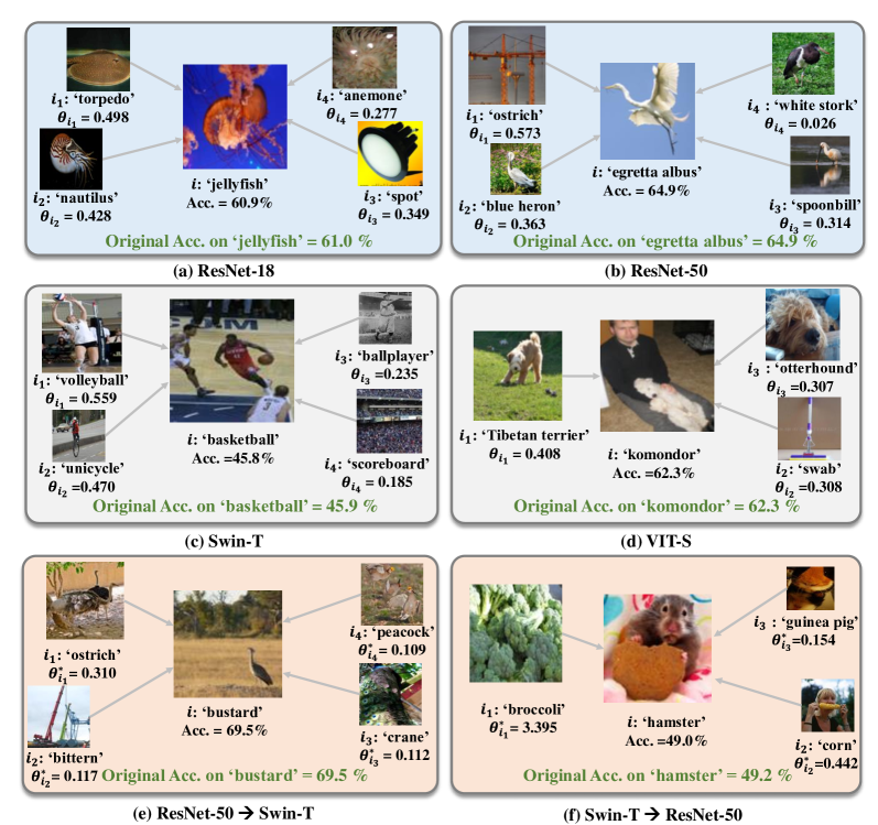
Figure 2: Neural dependencies in popular multi-class classification networks. (a;b;c) Within-network neural dependencies in ResNet18, ResNet50, Swin-Transformer and VIT-Transformer; (e;f) Between-network neural dependencies between ResNet50 and Swin-Transformer. Much more results can be found in appendix.

Table 1: Prediction error and classification accuracy of neural dependencies in cases in Fig. 2. Both the error of logits prediction and the loss in classification accuracy are tiny. Much more results can be found in appendix.

Metrics	ResNet-18	ResNet-50	Swin-T	VIT-S	R-50 $\to$ Swin-T	Swin-T $\to$ R-50
Abs Err	0.187	0.068	0.104	0.297	0.207	0.211
Rel Err (%)	2.568	1.063	0.926	4.276	1.776	3.939
Acc (Ori. Acc)	60.9 (61.0)	64.9 (64.9)	40.1 (40.1)	45.9 (45.9)	69.5 (69.5)	49.0 (49.2)
Pos Acc (Ori. Pos Acc)	72.0 (84.0)	92.0 (92.0)	94.0 (92.0)	96.0 (100.0)	94.0 (96.0)	94.0 (100.0)

2.2 What Brings Dependencies

After identifying the neural dependencies in deep networks, we are curious about why this intriguing phenomenon can broadly exist in different architectures. So we need a further understanding of the sources of it, which can be discovered through a careful analysis on Eq. 2. This section will reveal how a redundant covariance matrix for the terminal representations induces the neural dependencies.

Observe that $\mathbb{E}_{{\bm{x}}\sim p_{\rm{data}}}[\|{\bm{\theta}}^{T}f({\bm{x}})\|_{2}^{2}]={\bm{\theta}}^{T}\mathrm{Cov}{\bm{\theta}}$, where $\mathrm{Cov}=\mathbb{E}_{{\bm{x}}\sim p_{\rm{data}}}[f({\bm{x}})f({\bm{x}})^{T}]$ is the (uncerntralized and unnormalized) covariance matrix of the terminal representations. Let $\bm{err}_{i}({\bm{\theta}})={\bm{\theta}}^{T}\mathrm{Cov}{\bm{\theta}}$ be the predicting error of using coefficient ${\bm{\theta}}$ for category $c_{i}$, the property of Lasso regression indicates that (see proof in appendix) $\bm{err}_{i}({\bm{\theta}}^{*}(\lambda))$ is continuous about $\lambda$ and

$$\frac{\det[\mathrm{Cov}]}{\det[\mathrm{Cov}_{[n]\setminus i}^{[n]\setminus i}]} =\bm{err}_{i}({\bm{\theta}}^{*}(0)$$ (5)

$$\leq\bm{err}_{i}({\bm{\theta}}^{*}(\lambda))\leq\bm{err}_{i}({\bm{\theta}}^{*}(\lambda^{\prime}))$$

$$\leq\bm{err}_{i}({\bm{\theta}}^{*}(\lambda_{\rm{max}}))=\mathrm{Cov}_{i}^{i},$$

where $\lambda\leq\lambda^{\prime}$, and $\lambda_{max}=2\|\mathrm{Cov}_{[n]\setminus i}^{i}\|_{\infty}$ is the supremum of valid hyper-parameter $\lambda$, i.e., ${\bm{\theta}}^{*}(\lambda)=-{\bm{e}}_{i}=(\underbrace{0,\cdots,0}_{i-1},-1,0,\cdots,0),\forall\lambda\geq\lambda_{\rm{max}}$, and ${\bm{\theta}}^{*}(\lambda)\neq-{\bm{e}}_{i},\forall 0\leq\lambda<\lambda_{\rm{max}}$.

Regardless of the sparsity, to yield neural dependency for the target category $c_{i}$, we expect a very small $\bm{err}_{i}({\bm{\theta}}^{*}(\lambda))$. So if the lower bound $\bm{err}_{i}({\bm{\theta}}^{*}(0))$ is already far larger than $\epsilon\delta$, the predicting error can be too large to yield neural dependencies. Reversely, using the continuity of $\bm{err}_{i}({\bm{\theta}}^{*}(\lambda))$ about $\lambda$, we can know that if the lower bound $\bm{err}_{i}({\bm{\theta}}^{*}(0))$ is very small, then there should be a small $\lambda$ such that $\bm{err}_{i}({\bm{\theta}}^{*}(\lambda))$ is also very small. Eq. 2 can then bring neural dependencies to category $c_{i}$. (This need to exclude a trivial case where the predicting error upper bound $\mathrm{Cov}_{i}^{i}=\mathbb{E}_{{\bm{x}}\sim p_{\rm{data}}}[f({\bm{x}})_{i}^{2}]$ is already very small as it does not reveal any meaningful dependencies but that the network may be very unconfident about category $c_{i}$. While this is rare for well-trained networks, we leave the discussion of this case in appendix.)

So to have neural dependencies, we require the term $\bm{err}_{i}({\bm{\theta}}^{*}(0))$ to be as small as possible. For term $\bm{err}_{i}({\bm{\theta}}^{*}(0))$ we can have the following observations from two different perspectives (see appendix for deduction):

1. Information Volume: $\bm{err}_{i}({\bm{\theta}}^{*}(0))=\frac{\det[\mathrm{Cov}]}{\det[\mathrm{Cov}_{[n]\setminus i}^{[n]\setminus i}]}=\frac{{\rm Vol}(\mathrm{Cov})}{{\rm Vol}(\mathrm{Cov}_{[n]\setminus i}^{[n]\setminus i})}$ measures the ratio between the $n$-dimensional volumes of the parallelotope $\mathrm{Cov}$ and the $n-1$ dimensional volumes of $\mathrm{Cov}$ removing the $i$-th row and $i$-th column; if assume Gaussian distributions of random variable $f({\bm{x}}),{\bm{x}}\sim p_{\rm{data}}$, they are also the normalizing constants of the probability density of the terminal representations with and without the $i$-th category; this term measures the information loss while removing the $i$-th category and is small if the $i$-th row and $i$-th column of $\mathrm{Cov}$ carry little information and are redundant;

2. Geometry: $\bm{err}_{i}({\bm{\theta}}^{*}(0))=\frac{\det[\mathrm{Cov}]}{\det[\mathrm{Cov}_{[n]\setminus i}^{[n]\setminus i}]}=(\sum_{j=1}^{n}\frac{{\bm{\alpha}}_{j}^{2}}{\sigma_{j}^{2}})^{-1}$ which will be small if some ${\bm{\alpha}}_{j}$ corresponding to tiny $\sigma_{j}^{2}$ is large, where $\sigma_{1}^{2}\geq\cdots\geq\sigma_{n}^{2}$ are the eigenvalues of $\mathrm{Cov}$ and ${\bm{q}}_{1},\cdots,{\bm{q}}_{n}$ are the corresponding eigenvectors, ${\bm{\alpha}}_{j}=\langle{\bm{e}}_{i},{\bm{q}}_{j}\rangle,j\in[n]$; this further means that the $i$-th coordinate axis is close to the null space (linear subspace spanned by eigenvectors corresponding to tiny eigenvalues) of the covariance matrix $\mathrm{Cov}$, which suggests the $i$-th category is redundant geometrically.

Let $\frac{\det[\mathrm{Cov}]}{\det[\mathrm{Cov}_{[n]\setminus i}^{[n]\setminus i}]}$ be the metric for redundancy of category $c_{i}$, both perspectives lead to the same conclusion that:

Redundancy of the target category $c_{i}$ in the terminal representations brings it neural dependencies.

Remark 2

Unfortunately, though it can help us understand the intrinsic mechanism that brings neural dependencies, this principle is only intuitive in practice—we can not accurately calculate the value $\frac{\det[\mathrm{Cov}]}{\det[\mathrm{Cov}_{[n]\setminus i}^{[n]\setminus i}]}$ in most cases due to numerical instability. $\det[\mathrm{Cov}_{[n]\setminus i}^{[n]\setminus i}]$ tends to have some tiny singular values (smaller than ${\rm 1e-3}$), making the quotient operation extremely sensitive to minor numerical errors in computation, and thus often induces ${\rm NaN}$ results.

2.3 What Brings Sparsity

The last section omits the discussion of sparsity, which we want to study carefully in this section. We want to find a value that estimates whether two categories have neural dependencies, which we will show later is the (uncerntralized) covariance between the logits for two different categories.

The sparsity property, i.e., whether category $c_{j}$ is involved in the neural dependencies with $c_{i}$, can be identified by the KKT condition of Eq. 2. Let $\hat{\mathrm{Cov}}=\mathrm{Cov}_{[n]\setminus i}^{[n]\setminus i}$, $\hat{{\bm{\theta}}}={\bm{\theta}}_{[n]\setminus i}$, $\hat{{\bm{b}}}=\mathrm{Cov}_{[n]\setminus i}^{i}$, and $\hat{j}=j+{\bm{1}}_{(j>i)}$ such that $\hat{{\bm{\theta}}}_{j}={\bm{\theta}}_{\hat{j}}$, Eq. 2 then transfer into

$$\min_{\hat{{\bm{\theta}}}\in\mathbb{R}^{n-1}}\hat{{\bm{\theta}}}^{T}\hat{\mathrm{Cov}}\hat{{\bm{\theta}}}-2\hat{{\bm{b}}}^{T}\hat{{\bm{\theta}}}+\lambda\|\hat{{\bm{\theta}}}\|_{1}.$$ (6)

By KKT conditions, the optimal value is attained only if

$${\bm{0}}\in\hat{\mathrm{Cov}}\hat{{\bm{\theta}}}^{*}(\lambda)-\hat{{\bm{b}}}+\frac{\lambda}{2}\partial\|\hat{{\bm{\theta}}}\|_{1}.$$ (7)

and the sparsity can be estimated by the following proposition (see detailed deduction in appendix)

$$|\hat{\mathrm{Cov}}_{j}\hat{{\bm{\theta}}}^{*}(\lambda)-\hat{{\bm{b}}}_{j}|<\frac{\lambda}{2}\Rightarrow\hat{{\bm{\theta}}}^{*}(\lambda)_{j}=0,j\in[n-1].$$ (8)

This means that we can know whether two categories admit neural dependencies by estimating $|\hat{\mathrm{Cov}}_{j}\hat{{\bm{\theta}}}^{*}(\lambda)-\hat{{\bm{b}}}_{j}|$. A surprising fact is that the term $|\hat{\mathrm{Cov}}_{j}\hat{{\bm{\theta}}}^{*}(\lambda)-\hat{{\bm{b}}}_{j}|$ can actually be estimated without solving Eq. 2, but using the slope of the solution path of the Lasso problem. By convexity of Eq. 2, the slope of Eq. 2 admits the following bound.

Theorem 2

Let $\hat{\mathrm{Cov}}={\bm{Q}}{\bm{\Sigma}}{\bm{Q}}^{T}$ be the eigenvalue decomposition of $\hat{\mathrm{Cov}}$, and ${\bm{A}}={\bm{Q}}{\bm{\Sigma}}^{1/2}{\bm{Q}}^{T}$, then we have for $\lambda^{\prime},\lambda^{\prime\prime}\in[0,\lambda_{\rm{max}}]$,

$$|\frac{\hat{\mathrm{Cov}}_{j}\hat{{\bm{\theta}}}^{*}(\lambda^{\prime})-\hat{{\bm{b}}}_{j}}{\lambda^{\prime}}-\frac{\hat{\mathrm{Cov}}_{j}\hat{{\bm{\theta}}}^{*}(\lambda^{\prime\prime})-\hat{{\bm{b}}}_{j}}{\lambda^{\prime\prime}}|$$ (9)

$$\leq \|{\bm{A}}_{j}\|_{2}\|{\bm{A}}^{-T}\hat{{\bm{b}}}\|_{2}|\frac{1}{\lambda^{\prime}}-\frac{1}{\lambda^{\prime\prime}}|,j\in[n-1].$$

Remark 3

Using this theorem we can also get a finer estimation of the value of $\bm{err}_{i}(\hat{{\bm{\theta}}}^{*}(\lambda))$ than Eq. 5, see appendix for detail.

Using triangular inequality and the closed-form solution for $\lambda_{\rm{max}}$ ($\hat{{\bm{\theta}}}^{*}(\lambda_{\rm{}_{max}})={\bm{0}}$), we have for $j\in[n-1]$,

$$|\hat{\mathrm{Cov}}_{j}\hat{{\bm{\theta}}}^{*}(\lambda)-\hat{{\bm{b}}}_{j}|\leq\lambda|\frac{\hat{\mathrm{Cov}}_{j}\hat{{\bm{\theta}}}^{*}(\lambda_{\rm{max}})-\hat{{\bm{b}}}_{j}}{\lambda_{\rm{max}}}|$$ (10)

$$+ \lambda|\frac{\hat{\mathrm{Cov}}_{j}\hat{{\bm{\theta}}}^{*}(\lambda)-\hat{{\bm{b}}}_{j}}{\lambda}-\frac{\hat{\mathrm{Cov}}_{j}\hat{{\bm{\theta}}}^{*}(\lambda_{\rm{max}})-\hat{{\bm{b}}}_{j}}{\lambda_{\rm{max}}}|$$ (11)

$$\leq \lambda|\frac{\hat{{\bm{b}}}_{j}}{\lambda_{\rm{max}}}|+\lambda\|{\bm{A}}_{j}\|_{2}\|{\bm{A}}^{-T}\hat{{\bm{b}}}\|_{2}|\frac{1}{\lambda}-\frac{1}{2\|\hat{{\bm{b}}}\|_{\infty}}|.$$ (12)

Thus if $\lambda|\frac{\hat{{\bm{b}}}_{j}}{\lambda_{\rm{max}}}|+\lambda\|{\bm{A}}_{j}\|_{2}\|{\bm{A}}^{-T}\hat{{\bm{b}}}\|_{2}|\frac{1}{\lambda}-\frac{1}{2\|\hat{{\bm{b}}}\|_{\infty}}|<\frac{\lambda}{2}\Leftrightarrow|\frac{\hat{{\bm{b}}}_{j}}{\|\hat{{\bm{b}}}\|_{\infty}}|<1-2\|{\bm{A}}_{j}\|_{2}\|{\bm{A}}^{-T}\hat{{\bm{b}}}\|_{2}|\frac{1}{\lambda}-\frac{1}{2\|\hat{{\bm{b}}}\|_{\infty}}|$, we know that $\hat{{\bm{\theta}}}^{*}(\lambda)_{j}=0$ and category $c_{\hat{j}}$ is independent (meaning not involved in the neural dependencies) with $c_{i}$.

Theorem 3

When $0<\lambda<\lambda_{\rm{max}}$ and $\hat{j}\neq i$, if

$$\frac{|\mathbb{E}_{{\bm{x}}\sim p_{\rm{data}}}[f({\bm{x}})_{i}f({\bm{x}})_{\hat{j}}]|}{\max_{s\neq i}|\mathbb{E}_{{\bm{x}}\sim p_{\rm{data}}}[f({\bm{x}})_{i}f({\bm{x}})_{s}]|}$$ (13)

$$< 1-2\|{\bm{A}}_{j}\|_{2}\|{\bm{A}}^{-T}\hat{{\bm{b}}}\|_{2}|\frac{1}{\lambda}-\frac{1}{2\|\hat{{\bm{b}}}\|_{\infty}}|,$$

then ${\bm{\theta}}^{*}(\lambda)_{\hat{j}}=0$ and category $c_{\hat{j}}$ is independent with $c_{i}$.

High dimensional vectors are known to tend to be orthogonal to each other [4], thus if we assume ${\bm{A}}_{j}$ is nearly orthogonal to ${\bm{A}}^{-T}\hat{{\bm{b}}}$, then $\|{\bm{A}}_{j}\|_{2}\|{\bm{A}}^{-T}\hat{{\bm{b}}}\|_{2}\approx|\hat{{\bm{b}}}_{j}|$ and we can further simplify the above sparsity criterion as

Conjecture 1

When $0<\lambda<\lambda_{\rm{max}}$ and $j\neq i$, if

$$|\mathbb{E}_{{\bm{x}}\sim p_{\rm{data}}}[f({\bm{x}})_{i}f({\bm{x}})_{j}]|<\frac{\lambda}{2}(\text{equivalent to }$$ (14)

$$\frac{|\mathbb{E}_{{\bm{x}}\sim p_{\rm{data}}}[f({\bm{x}})_{i}f({\bm{x}})_{j}]}{\max_{s\neq i}|\mathbb{E}_{{\bm{x}}\sim p_{\rm{data}}}[f({\bm{x}})_{i}f({\bm{x}})_{s}]|}|<\frac{\lambda}{\lambda_{\rm{max}}}),$$

then ${\bm{\theta}}^{*}(\lambda)_{j}=0$ and category $c_{j}$ is independent with $c_{i}$.

In practice we find that this conjecture is seldom wrong. Combining with Theorem 3, they together tell us that the covariance of terminal representations has an important role in assigning neural dependencies: more correlated categories tend to have neural dependencies, while weakly correlated categories will not have neural dependencies. They also describe the role of the hyper-parameter $\lambda$ in Eq. 2: it screens out less correlated categories when searching neural dependencies, and larger $\lambda$ corresponds to higher sparsity of dependencies. In conclusion, let $|\mathbb{E}_{{\bm{x}}\sim p_{\rm{data}}}[f({\bm{x}})_{i}f({\bm{x}})_{j}]|$ be the metric for correlations between category $c_{i}$ and $c_{j}$, we can say that

Low covariance between categories in the terminal representations brings sparsity of dependencies.

Numerical Validation.

We validate the above principle, i.e., Conject. 1 in Fig. 3. Each subfigure picks up one target category $c_{i}$ and solves Eq. 2 to calculate the corresponding coefficients ${\bm{\theta}}_{j}^{*},j\neq i$ for all the remaining 999 categories of the ImageNet. ${\bm{\theta}}^{*}_{j}=0$ implies no neural dependency between category $c_{i}$ and $c_{j}$, and vice versa. We plot the relation between the covariance of $c_{i},c_{j}$, $|\mathbb{E}_{{\bm{x}}\sim p_{\rm{data}}}[f({\bm{x}})_{i}f({\bm{x}})_{j}]|$, and the corresponding dependency coefficient ${\bm{\theta}}_{j}^{*}$. We can clearly find out that a small correlation corresponds to no neural dependency. Specifically, when the correlation between $c_{i},c_{j}$ is smaller than $\frac{\lambda}{2}$, $c_{i}$ and $c_{j}$ admit no neural dependency. In most cases, the bar $\frac{\lambda}{2}$ does exclude a considerable amount of zero dependency categories, which makes it a good indicator for the existence of neural dependency. This validates our principle for the source of sparsity.

Controlling Neural Dependencies.

Conject. 1 also points out that we can disentangle neural dependencies by regularizing the covariance term, as tiny covariance of $|\mathbb{E}_{{\bm{x}}\sim p_{\rm{data}}}[f({\bm{x}})_{i}f({\bm{x}})_{j}]|$ indicates no neural dependency between category $c_{i}$ and $c_{j}$. We will discuss this later in Sec. 3.3.

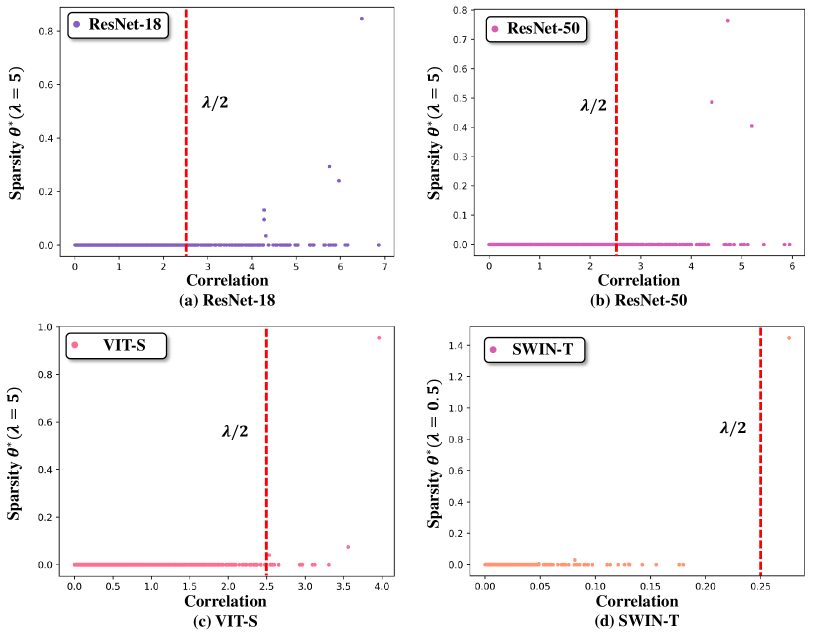
Figure 3: Relation between correlations and dependency coefficients.

2.4 Between Network Neural Dependencies

The general math property of the between network neural dependencies shows no essential difference from the within network ones. Let $f,g$ be two different classification neural networks trained on $p_{\rm{data}}$ independently. We want to use the logits of $f$ to predict the logits of the $c_{i}$ category of $g$. Let $\tilde{f}({\bm{x}})=(f({\bm{x}})_{1},\cdots,f({\bm{x}})_{i-1},g({\bm{x}})_{i},f({\bm{x}})_{i+1},\cdots,f({\bm{x}})_{n})^{T}$, and $\tilde{\mathrm{Cov}}=\mathbb{E}_{{\bm{x}}\sim p_{\rm{data}}}[\tilde{f}({\bm{x}})\tilde{f}({\bm{x}})^{T}]$, then we know that

• if $\frac{\det[\tilde{\mathrm{Cov}}]}{\det[\tilde{\mathrm{Cov}}]_{[n]\setminus i}^{[n]\setminus i}}=\frac{\det[\tilde{\mathrm{Cov}}]}{\det[\mathrm{Cov}_{[n]\setminus i}^{[n]\setminus i}]}$ is small, then category $c_{i}$ of network $g$ have neural dependencies with some other categories of network $f$;

• if $|\mathbb{E}_{{\bm{x}}\sim p_{\rm{data}}}[f({\bm{x}})_{j}g({\bm{x}})_{i}]|$ ($j\neq i$) is small, then the $c_{j}$ category of $f$ is independent with the $c_{i}$ category of $g$.

3 Potentials of Neural Dependencies

In this section, we discuss some interesting potentials and inspirations of neural dependencies in general scenarios of modern machine learning.

3.1 Visualization Neural Dependencies

We are curious about the intrinsic data relations revealed by neural dependencies. Specifically, if we have some base classes in the coordinate space, can we plot the position of the target classes that can be linearly decided by (have neural dependencies with) those classes? Fig. 4 gives such an example for ResNet-50 in ImageNet. In the surroundings are 88 base categories and in the center are 10 target categories that can be linearly predicted by them using neural dependencies. The length of the arc between two categories gives their dependency coefficient. This result illustrates the relative relationship of different categories acknowledged by the neural network. It may be of potential interests to multiple domains like data relation mining, visualization, and interpretability of deep networks.

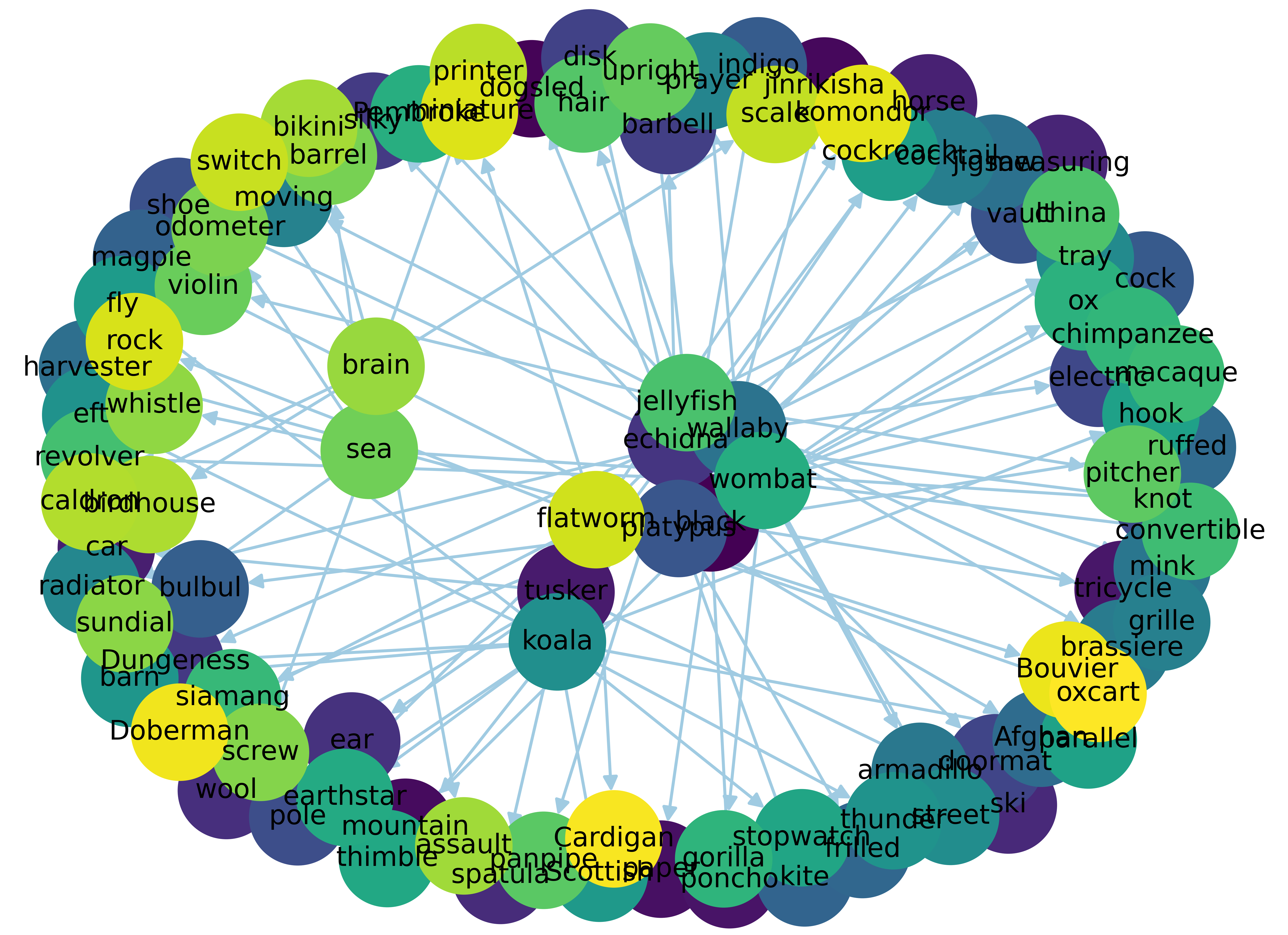
Figure 4: The graph visualization of neural dependencies in a pretrained ResNet-50. Please refer to Sec. 3.1 for detail.

Table 2: Classification accuracy of baselines and learning new categories through neural dependencies (ours). While much simpler, learning new categories through neural dependencies barely looses accuracy. All figures are the mean of five independent runs.

	$900\to 100$			$950\to 50$			$999\to 1$			$999\to 1(pos\&neg)$
Backbone	Baseline	Ours	Impro	Baseline	Ours	Impro	Baseline	Ours	Impro	Baseline	Ours	Impro
ResNet50	68.47	68.03	-0.44	68.47	68.45	-0.02	68.47	68.46	-0.01	60.70	61.50	+0.80
Swin-T	71.49	71.486	-0.004	71.49	71.578	+0.088	71.49	71.56	+0.07	76.20	78.00	+1.80

Table 3: Metrics of using (ours) and not using (baselines) the dependency regularization. All figures are mean of five independent runs.

	ImageNet Acc. $(\uparrow)$			Dependency Coefficients $(\downarrow)$			ImageNet-O AUPR $(\uparrow)$
Backbone	Baseline	Ours	Impro	Baseline	Ours	Impro	Baseline	Ours	Impro
ResNet18	69.83	70.12	+0.29	0.70	0.02	+0.68	15.15	15.48	+0.33
ResNet50	76.37	76.66	+0.29	1.10	$4.5e^{-4}$	+1.10	13.98	14.07	+0.09
Vit-S	80.67	81.52	+0.85	0.1	$3.1e^{-3}$	+0.1	28.54	31.14	+2.60
Swin-T	82.16	82.18	+0.02	0.39	0.01	+0.38	27.66	28.13	+0.47

Table 4: Classification accuracy in base (900) and new (100) categories separately. While much simpler, learning new categories through neural dependencies outperform baselines if only consider the performance in the new categories. All figures are mean of five independent runs.

	ResNet-50		Swin-T
Method	900	100	900	100
Baseline	72.54	36.94	71.42	72.04
Ours	72.89	48.90	71.36	74.63

3.2 Generalizability

Now that the logits of one category can be well predicted by the logits of some others, we are curious about whether we can learn a cluster of base categories, and then predict new classes purely using linear combinations of the logits of those base categories. Especially, can the overall performance of this setting be comparable to training the baseline model on the whole dataset? This problem is of general interest to many machine learning scenarios. 1) Incremental Learning. In incremental learning [25, 15, 5] we need to learn to predict novel categories using a pretrained network on old categories. Typical methods will finetune the pretrained network in the new categories to achieve this goal, which then arouses concerns of damaging the knowledge of the old categories. Using our setting we can explore the potential of keeping the pretrained network unchanged and learning merely a small weight matrix to handle novel categories, which is cheap and efficient to train and deploy in various devices and realistic scenarios. 2) Transfer Learning. A similar but different occasion is transfer learning [16, 23, 22], where we seek to take advantage of knowledge of old domains to improve performance in new data domains. While categories are also instances of domains, our setting also explores a new way of knowledge transfer among domains. 3) Representation Learning. Our setting can partially reveal how representations [1] of base knowledge help classifications in out-of-distribution data (new categories). Future studying of this setting may reveal the source of the generalizability of neural networks from the perspective of neural dependencies.

To implement our setting, we may first train a deep classification network $f_{\rm base}:{\mathbb{R}}^{m}\rightarrow{\mathbb{R}}^{n_{1}}$ on the $n_{1}$ base categories. Then we learn a coefficient matrix $\bm{\Theta}\in{\mathbb{R}}^{n_{1}\times n_{2}}$ by fixing the parameters of $f_{\rm base}$ and minimizing the training loss of $f_{\rm new}=f_{\rm base}\bm{\Theta}$ on the training set of the new categories. We then concatenate $f_{\rm all}=[f_{\rm base},f_{\rm base}\bm{\Theta}]^{T}$ to form a new classifier for all the categories. We sample 500 samples per category from the trainset of ImageNet-1k as our training data; the remains are used for constructing a balanced binary testing set we will use later. We evaluate the following three settings: 1) from 900 base classes to 100 new classes ($900\to 100$), 2) from 950 base classes to 50 new classes ($950\to 50$), and 3) from 999 base classes to 1 new class ($999\to 1$) within a dataset. To approach a binary classification scenario, for $999\to 1$ case we additionally test on 500 positive and negative sample pairs from the remained trainset of ImageNet as the $999\to 1(pos\&neg)$ setting. The baselines $f_{\rm baseline}$ are backbone models trained on the whole 1,000 category training data. Other details can be found in appendix.

Experimental Results. We report the performance of $f_{\rm all}$ and $f_{\rm baseline}$ in Tab. 2, where we can find both settings (ours v.s. baselines) achieve comparable performance. While our setting requires training on only a small coefficient matrix, it consumes much less computation and time resources (less than 60% time consumption of the baseline in each epoch, see appendix for detail) compared with the baselines. We further investigate how our setting performs in the new categories. Tab. 4 reports classification accuracy in the old 900 and new 100 categories of our setting and baselines (here we choose the class with maximum logits in the 900/100 categories as the prediction results). We can find that our setting significantly outperforms the baselines in the new classes. Both results reveal the power of neural dependencies in the generalizability of deep networks.

3.3 Robustness

As we have mentioned before, some neural dependencies are not that sensible for humans. We are therefore curious about whether cutting off those dependencies can help the network and improve robustness. Here we compare two cases, the baselines and baselines finetuned by adding the regularization term $|\mathbb{E}_{{\bm{x}}\sim p_{\rm{data}}}[f({\bm{x}})_{i}f({\bm{x}})_{j}]|$ where $c_{i},c_{j}$ are the two categories that emerge irrational neural dependencies to cut off. We use two benchmarks, ImageNet-1k and ImageNet-O [11]. ImageNet-O consists of images from 200 classes that are unseen in ImageNet-1k, and is used to test the robustness of networks to out-of-distribution samples. This ability is usually measured by the AUPR (i.e., area under the precision-recall curve) metric [2]. This metric requires anomaly scores, which is the negative of the maximum softmax probabilities from a model that can classify the 200 classes. We train the baseline models for 90 epochs and our settings for 60 epochs of regular training followed by 30 epochs of finetuning using the regularization term $|\mathbb{E}_{{\bm{x}}\sim p_{\rm{data}}}[f({\bm{x}})_{i}f({\bm{x}})_{j}]|$. We manually choose one dependency to cut off for each case. Details can be found in appendix.

Experimental Results. Tab. 3 reports the results. The regularization term does cut off the neural dependencies as the dependency coefficients are approaching zero after regularization. This then results in some improvements of performance in both ImageNet and ImageNet-O for all the backbones. While here we only cut-off one dependency for each case, we believe a thorough consideration of reasonable dependencies to maintain may benefit the network more. This reveals the connection between neural dependencies and the robustness of networks.

4 Conclusion

This paper reveals an astonishing neural dependency phenomenon emerging from learning massive categories. Given a well-trained model, the logits predicted for some category can be directly obtained by linearly combining the predictions of a few others. Theoretical investments demonstrate how to find those neural dependencies precisely, when they happen, and why the dependency is usually sparse, i.e. only a few instead of numerous of other categories related to one target category. Further empirical studies reveal multiple attractive potentials of neural dependencies from the aspects of visualization, generalization, and robustness of deep classification networks.

Appendix A Proof

A.1 Proof to Theorem 1

This is the natural results of Eq. 3.

A.2 Property of Function $\bm{err}_{i}({\bm{\theta}}^{*}(\lambda))$

The continuity of the solution path and the existence of $\lambda_{\rm{max}}=2\|\mathrm{Cov}_{[n]\setminus i}^{i}\|_{\infty}$ are natural results of the property of general Lasso regressions [19, 20]. Here we prove that

$$\bm{err}_{i}({\bm{\theta}}^{*}(0)=\frac{\det[\mathrm{Cov}]}{\det[\mathrm{Cov}_{[n]\setminus i}^{[n]\setminus i}]},$$ (A15)

$$\bm{err}_{i}({\bm{\theta}}^{*}(\lambda_{\rm{max}}))=\mathrm{Cov}_{i}^{i}.$$ (A16)

In fact, the second equality Eq. A16 is easy to verify directly, so we only need to prove the first one, Eq. A15. Let

$$\mathrm{Cov}=\bm{U}\bm{\Gamma}\bm{U}^{T},$$ (A17)

$$\bm{U}\bm{U}^{T}=\bm{I},$$ (A18)

$$\bm{\Gamma}={\rm{diag}}\{\gamma_{1}^{2},\cdots,\gamma_{n}^{2}\},$$ (A19)

$${\bm{\theta}}=\sum_{j=1}^{n}\bm{\alpha}_{j}\bm{U}^{j},$$ (A20)

$${\bm{\theta}}_{i}=\sum_{j=1}^{n}\bm{\alpha}_{j}\bm{U}^{j}_{i}=\bm{U}_{i}\bm{\alpha}=-1,$$ (A21)

and $\bm{U}^{1},\cdots,\bm{U}^{n}$ be the eigenvectors of $\mathrm{Cov}$. The original problem Eq. 2 (when $\lambda=0$) now becomes

$$\min_{\bm{\alpha}}\sum_{j=1}^{n}\bm{\alpha}_{j}^{2}\gamma_{j}^{2},$$ (A22)

$$~{}\text{subject to }\sum_{j=1}^{n}\bm{\alpha}_{j}\bm{U}^{j}_{i}=-1.$$

Using Lagrange multiplier, the following problem will attain extreme value together with the above problem

$$\min_{\bm{\alpha},\eta}H(\bm{\alpha},\eta)=\sum_{j=1}^{n}\bm{\alpha}_{j}^{2}\gamma_{j}^{2}+\eta(\sum_{j=1}^{n}\bm{\alpha}_{j}\bm{U}^{j}_{i}+1).$$ (A23)

Thus we have

$$\frac{\partial H}{\partial\bm{\alpha}_{j}}=2\bm{\alpha}_{j}\gamma_{j}^{2}+\eta\bm{U}_{i}^{j}=0\Leftrightarrow\bm{\alpha}_{j}=-\frac{\eta\bm{U}_{i}^{j}}{2\gamma_{j}^{2}},j=1,\cdots,n,$$ (A24)

$$\Leftrightarrow\bm{\alpha}=-\frac{\eta}{2}\bm{\Gamma}^{-1}\bm{U}_{i}^{T}=-\frac{\eta}{2}\bm{\Gamma}^{-1}\bm{U}^{T}\bm{e}_{i}$$ (A25)

$$\frac{\partial H}{\partial\eta}=\sum_{j=1}^{n}\bm{\alpha}_{j}\bm{U}^{j}_{i}+1=0\Leftrightarrow\sum_{j=1}^{n}-\frac{\eta\bm{U}_{i}^{j}}{2\gamma_{j}^{2}}\bm{U}_{i}^{j}=-1\Leftrightarrow\frac{\eta}{2}\sum_{j=1}^{n}\frac{(\bm{U}_{i}^{j})^{2}}{\gamma_{j}^{2}}=1$$ (A26)

$$\Leftrightarrow\eta=2(\bm{U}_{i}\bm{\Gamma}^{-1}\bm{U}_{i}^{T})^{-1}=2(\bm{e}_{i}^{T}\bm{U}\bm{\Gamma}^{-1}\bm{U}^{T}\bm{e}_{i})^{-1}=2/(\mathrm{Cov}^{-1})_{i}^{i}.$$ (A27)

Combining the above derivation, we have

$${\bm{\theta}}^{*}(0)=\bm{U}\bm{\alpha}^{*}=-\frac{\eta}{2}\bm{U}\bm{\Gamma}^{-1}\bm{U}^{T}\bm{e}_{i}=-\frac{\eta}{2}\mathrm{Cov}^{-1}\bm{e}_{i},$$ (A28)

$$({\bm{\theta}}^{*}(0)^{T}\mathrm{Cov}{\bm{\theta}}^{*}(0))=\frac{\eta^{2}}{4}\bm{e}_{i}^{T}\mathrm{Cov}^{-T}\mathrm{Cov}\mathrm{Cov}^{-1}\bm{e}_{i}=\frac{\eta^{2}}{4}\bm{e}_{i}^{T}\mathrm{Cov}^{-1}\bm{e}_{i}$$ (A29)

$$=\frac{\eta^{2}}{4}(\mathrm{Cov}^{-1})_{i}^{i}=1/(\mathrm{Cov}^{-1})_{i}^{i}=\frac{\det[\mathrm{Cov}]}{\det[\mathrm{Cov}_{[n]\setminus i}^{[n]\setminus i}]}.$$ (A30)

A.3 Case of Small $\mathrm{Cov}_{i}^{i}$

Here we may want the ratio

$${\mathcal{R}}(\mathrm{Cov},i)=\frac{\det[\mathrm{Cov}]}{\mathrm{Cov}_{i}^{i}\det[\mathrm{Cov}_{[n]\setminus i}^{[n]\setminus i}]}=\frac{1}{\sum_{j=1}^{n}\frac{{\bm{\alpha}}_{j}^{2}}{\sigma_{j}^{2}}\sum_{j=1}^{n}{\bm{\alpha}}_{j}^{2}\sigma_{j}^{2}}$$ (A31)

to be as small as possible, where $\sigma_{1}^{2}\geq\cdots\geq\sigma_{n}^{2}$ are the eigenvalues of $\mathrm{Cov}$ and ${\bm{q}}_{1},\cdots,{\bm{q}}_{n}$ are the corresponding eigenvectors, $\alpha_{j}=\langle{\bm{e}}_{i},{\bm{q}}_{j}\rangle,j\in[n]$ (refer to deduction in Appendix). This is also the minimum relative prediction error, i.e.,

$$\inf_{\lambda\geq 0}\frac{\mathbb{E}_{{\bm{x}}\sim p_{\rm{data}}}[|f({\bm{x}})_{i}-\sum_{j\neq i}{\bm{\theta}}^{*}(\lambda)_{j}f({\bm{x}})_{j}|^{2}]}{\mathbb{E}_{{\bm{x}}\sim p_{\rm{data}}}[|f({\bm{x}})_{i}|^{2}]}={\mathcal{R}}(\mathrm{Cov},i),\forall\lambda\in[0,\lambda_{\rm{max}}].$$ (A32)

Geometrically, this means that the $i$-th coordinate axis admits valid components in the eigenvectors of both non-tiny and tiny eigenvalues.

A.4 Property of the Lower Bound $\bm{err}_{i}({\bm{\theta}}^{*}(0))$

Here we prove that

$$\bm{err}_{i}({\bm{\theta}}^{*}(0))=\frac{\det[\mathrm{Cov}]}{\det[\mathrm{Cov}_{[n]\setminus i}^{[n]\setminus i}]}=\left(\sum_{j=1}^{n}\frac{{\bm{\alpha}}_{j}^{2}}{\sigma_{j}^{2}}\right)^{-1}.$$ (A33)

This is the natural result of Eqs. A26 and A27, as

$$1/(\mathrm{Cov}^{-1})_{i}^{i}=\frac{\det[\mathrm{Cov}]}{\det[\mathrm{Cov}_{[n]\setminus i}^{[n]\setminus i}]}=1/(\mathrm{Cov}^{-1})_{i}^{i}=\frac{\eta}{2}=\left(\sum_{j=1}^{n}\frac{(\bm{U}_{i}^{j})^{2}}{\gamma_{j}^{2}}\right)^{-1}.$$ (A34)

Let ${\bm{U}}^{j}={\bm{q}}_{j}$ and $\sigma_{j}^{2}=\gamma_{j}^{2}$. Then we obtain the result.

A.5 Sparsity Condition of the Solution

By KKT conditions, the optimal value of Eq. 6 is attained only if

$${\bm{0}}\in\hat{\mathrm{Cov}}\hat{{\bm{\theta}}}^{*}(\lambda)-\hat{{\bm{b}}}+\frac{\lambda}{2}\partial\|\hat{{\bm{\theta}}}\|_{1}$$ (A35)

where $\partial\|\hat{{\bm{\theta}}}\|_{1}=\{{\bm{v}}:\|{\bm{v}}\|_{\infty}\leq 1,{\bm{v}}^{T}\hat{{\bm{\theta}}}=\|\hat{{\bm{\theta}}}\|_{1}\}$ is the subgradient of $\|\cdot\|_{1}$. By Cauchy inequality,

$$\|\hat{{\bm{\theta}}}\|_{1}={\bm{v}}^{T}\hat{{\bm{\theta}}}\leq\|{\bm{v}}\|_{\infty}\|\hat{{\bm{\theta}}}\|_{1}=\|\hat{{\bm{\theta}}}\|_{1}.$$ (A36)

The equality holds if and only if

$$|{\bm{v}}_{i}|<1\Rightarrow\hat{{\bm{\theta}}}_{i}=0.$$ (A37)

Thus we have the sparsity condition of the solution.

A.6 Proof to Eq. 9

To start, we deduce the dual problem of Eq. 2. For standard Lasso problem

$$\min_{\bm{\beta}}\frac{1}{2}\|\bm{y}-\bm{X}\bm{\beta}\|_{2}^{2}+\lambda\|\bm{\beta}\|_{1},$$ (A38)

where ${\bm{y}}$ are labels and ${\bm{X}}$ are observations, its dual problem is [20]

$$\max_{\bm{\xi}}\frac{1}{2}\|\bm{y}\|_{2}^{2}-\frac{\lambda^{2}}{2}\|\bm{\xi}-\frac{\bm{y}}{\lambda}\|_{2},$$ (A39)

$$\text{ subject to }|(\bm{X}^{j})^{T}\bm{\xi}|\leq 1,j=1,\cdots,n.$$

Let

$$\hat{\mathrm{Cov}}=\bm{Q}\bm{\Sigma}\bm{Q}^{T},$$ (A40)

$$\bm{A}=\bm{Q}\bm{\Sigma}^{1/2}\bm{Q}^{T},$$ (A41)

$$\hat{{\bm{b}}}=\mathrm{Cov}_{[n]\setminus i}^{i},$$ (A42)

$$\bm{y}=\sqrt{2}\bm{A}^{-T}\hat{{\bm{b}}},$$ (A43)

$$\text{and}~{}\bm{X}=\sqrt{2}\bm{A}.$$ (A44)

We then get the dual problem of Eqs. 2 and 6 as

$$\max_{\bm{\xi}}\|\bm{A}^{-1}\hat{{\bm{b}}}\|_{2}^{2}-\frac{\lambda^{2}}{2}\|\bm{\xi}-\frac{\sqrt{2}\bm{A}^{-T}\hat{{\bm{b}}}}{\lambda}\|_{2}^{2},$$ (A45)

$$\text{ subject to }\|\bm{A}\bm{\xi}\|_{\infty}\leq\frac{\sqrt{2}}{2}.$$

By the KKT condition, we further have

$$\sqrt{2}\bm{A}^{-T}\hat{{\bm{b}}}=\sqrt{2}\bm{A}\hat{{\bm{\theta}}}^{*}(\lambda)+\lambda\bm{\xi}^{*}(\lambda),$$ (A46)

$$\text{when }\lambda\geq\lambda_{\rm{max}}=\|\sqrt{2}\bm{A}\sqrt{2}\bm{A}^{-T}\hat{{\bm{b}}}\|_{\infty}=2\|\hat{{\bm{b}}}\|_{\infty},\hat{{\bm{\theta}}}^{*}=\bm{0}.$$ (A47)

The dual problem Eq. A45 can be further transferred into

$$\min_{\bm{\xi}}\|\bm{\xi}-\frac{\sqrt{2}\bm{A}^{-T}\hat{{\bm{b}}}}{\lambda}\|_{2}^{2},$$ (A48)

$$\text{ subject to }\|\bm{A}\bm{\xi}\|_{\infty}\leq\frac{\sqrt{2}}{2}.$$

This problem solves the projection of point $\frac{\sqrt{2}\bm{A}^{-T}\hat{{\bm{b}}}}{\lambda}$ onto the convex set $\{\bm{\xi}:\|\bm{A}\bm{\xi}\|_{\infty}\leq\frac{\sqrt{2}}{2}\}$. Denote its solution as $\bm{\xi}^{*}(\lambda)$ for parameter $\lambda$. It is then easy to verify

$$\|\frac{\sqrt{2}{\bm{A}}^{-T}\hat{{\bm{b}}}}{\lambda^{\prime\prime}}-\frac{\sqrt{2}{\bm{A}}^{-T}\hat{{\bm{b}}}}{\lambda^{\prime}}\|_{2}^{2}=\|\bm{\xi^{*}}(\lambda^{\prime\prime})-\bm{\xi^{*}}(\lambda^{\prime})-\bm{\xi}^{*}(\lambda^{\prime\prime})+\frac{\sqrt{2}{\bm{A}}^{-T}\hat{{\bm{b}}}}{\lambda^{\prime\prime}}+\bm{\xi}^{*}(\lambda^{\prime})-\frac{\sqrt{2}{\bm{A}}^{-T}\hat{{\bm{b}}}}{\lambda^{\prime}}\|_{2}^{2}$$ (A49)

$$=\|\bm{\xi^{*}}(\lambda^{\prime\prime})-\bm{\xi^{*}}(\lambda^{\prime})\|_{2}^{2}+\|\bm{\xi}^{*}(\lambda^{\prime\prime})-\frac{\sqrt{2}{\bm{A}}^{-T}\hat{{\bm{b}}}}{\lambda^{\prime\prime}}\|_{2}^{2}+\|\bm{\xi}^{*}(\lambda^{\prime})-\frac{\sqrt{2}{\bm{A}}^{-T}\hat{{\bm{b}}}}{\lambda^{\prime}}\|_{2}^{2}$$ (A50)

$$+2\langle\bm{\xi}^{*}(\lambda^{\prime\prime})-\bm{\xi}^{*}(\lambda^{\prime}),\frac{\sqrt{2}{\bm{A}}^{-T}\hat{{\bm{b}}}}{\lambda^{\prime\prime}}-\bm{\xi}^{*}(\lambda^{\prime\prime})\rangle+2\langle\bm{\xi}^{*}(\lambda^{\prime\prime})-\bm{\xi}^{*}(\lambda^{\prime}),\bm{\xi}^{*}(\lambda^{\prime})-\frac{\sqrt{2}{\bm{A}}^{-T}\hat{{\bm{b}}}}{\lambda^{\prime}}\rangle$$ (A51)

$$+2\langle\frac{\sqrt{2}{\bm{A}}^{-T}\hat{{\bm{b}}}}{\lambda^{\prime\prime}}-\bm{\xi}^{*}(\lambda^{\prime\prime}),\bm{\xi}^{*}(\lambda^{\prime})-\frac{\sqrt{2}{\bm{A}}^{-T}\hat{{\bm{b}}}}{\lambda^{\prime}}\rangle$$ (A52)

$$=\|\bm{\xi^{*}}(\lambda^{\prime\prime})-\bm{\xi^{*}}(\lambda^{\prime})\|_{2}^{2}+\|\bm{\xi}^{*}(\lambda^{\prime\prime})-\frac{\sqrt{2}{\bm{A}}^{-T}\hat{{\bm{b}}}}{\lambda^{\prime\prime}}-\bm{\xi}^{*}(\lambda^{\prime})-\frac{\sqrt{2}{\bm{A}}^{-T}\hat{{\bm{b}}}}{\lambda^{\prime}}\|_{2}^{2}$$ (A53)

$$+2\langle\bm{\xi}^{*}(\lambda^{\prime\prime})-\bm{\xi}^{*}(\lambda^{\prime}),\frac{\sqrt{2}{\bm{A}}^{-T}\hat{{\bm{b}}}}{\lambda^{\prime\prime}}-\bm{\xi}^{*}(\lambda^{\prime\prime})\rangle+2\langle\bm{\xi}^{*}(\lambda^{\prime\prime})-\bm{\xi}^{*}(\lambda^{\prime}),\bm{\xi}^{*}(\lambda^{\prime})-\frac{\sqrt{2}{\bm{A}}^{-T}\hat{{\bm{b}}}}{\lambda^{\prime}}\rangle$$ (A54)

$$\geq\|\bm{\xi^{*}}(\lambda^{\prime\prime})-\bm{\xi^{*}}(\lambda^{\prime})\|_{2}^{2}.$$ (A55)

The last inequality uses the fact that

$$2\langle\bm{\xi}^{*}(\lambda^{\prime\prime})-\bm{\xi}^{*}(\lambda^{\prime}),\frac{\sqrt{2}{\bm{A}}^{-T}\hat{{\bm{b}}}}{\lambda^{\prime\prime}}-\bm{\xi}^{*}(\lambda^{\prime\prime})\rangle\geq 0,$$ (A56)

$$2\langle\bm{\xi}^{*}(\lambda^{\prime\prime})-\bm{\xi}^{*}(\lambda^{\prime}),\bm{\xi}^{*}(\lambda^{\prime})-\frac{\sqrt{2}{\bm{A}}^{-T}\hat{{\bm{b}}}}{\lambda^{\prime}}\rangle\geq 0,$$ (A57)

for convex set $\{\bm{\xi}:\|\bm{A}\bm{\xi}\|_{\infty}\leq\frac{\sqrt{2}}{2}\}$ and the projections $\bm{\xi}^{*}(\lambda^{\prime}),\bm{\xi}^{*}(\lambda^{\prime\prime})$ on it. Thus we have

$$\|\bm{\xi^{*}}(\lambda^{\prime\prime})-\bm{\xi^{*}}(\lambda^{\prime})\|_{2}\leq\|\frac{\sqrt{2}{\bm{A}}^{-T}\hat{{\bm{b}}}}{\lambda^{\prime\prime}}-\frac{\sqrt{2}{\bm{A}}^{-T}\hat{{\bm{b}}}}{\lambda^{\prime}}\|_{2}.$$ (A58)

Combining Eq. A46, we then get the result of this theorem.

A.7 Finer Estimation of the Value of $\bm{err}_{i}({\bm{\theta}}^{*}(\lambda))$

We have

$$|{\bm{\theta}}^{*}(\lambda^{\prime\prime})^{T}\mathrm{Cov}{\bm{\theta}}^{*}(\lambda^{\prime\prime})-{\bm{\theta}}^{*}(\lambda^{\prime})^{T}\mathrm{Cov}{\bm{\theta}}^{*}(\lambda^{\prime})|$$ (A59)

$$=|\hat{{\bm{\theta}}}^{*}(\lambda^{\prime\prime})^{T}\hat{\mathrm{Cov}}\hat{{\bm{\theta}}}^{*}(\lambda^{\prime\prime})-\hat{{\bm{\theta}}}^{*}(\lambda^{\prime})^{T}\hat{\mathrm{Cov}}\hat{{\bm{\theta}}}^{*}(\lambda^{\prime})-2\hat{{\bm{b}}}^{T}(\hat{{\bm{\theta}}}^{*}(\lambda^{\prime\prime})-\hat{{\bm{\theta}}}^{*}(\lambda^{\prime}))|$$ (A60)

$$=|\|\bm{A}\hat{{\bm{\theta}}}^{*}(\lambda^{\prime\prime})-\bm{A}^{-T}\hat{{\bm{b}}}\|_{2}^{2}-\|\bm{A}\hat{{\bm{\theta}}}^{*}(\lambda^{\prime})-\bm{A}^{-T}\hat{{\bm{b}}}\|_{2}^{2}|$$ (A61)

$$=|\frac{\lambda^{\prime\prime 2}}{2}\|\bm{\xi}^{*}(\lambda^{\prime\prime})\|_{2}^{2}-\frac{\lambda^{\prime 2}}{2}\|\bm{\xi}^{*}(\lambda^{\prime})\|_{2}^{2}|.$$ (A62)

Setting $\lambda^{\prime}=\lambda_{\rm{max}},\lambda^{\prime\prime}=\lambda$, we can have

$$0\leq\mathrm{Cov}_{i}^{i}-{\bm{\theta}}^{*}(\lambda)^{T}\mathrm{Cov}{\bm{\theta}}^{*}(\lambda)=\|\bm{A}^{-T}\hat{{\bm{b}}}\|_{2}^{2}-\frac{\lambda^{2}}{2}\|\bm{\xi}^{*}(\lambda)\|_{2}^{2}$$ (A63)

$$\leq\|\bm{A}^{-T}\hat{{\bm{b}}}\|_{2}^{2}-\frac{\lambda^{2}}{2}(\|\frac{\sqrt{2}}{2\|\hat{{\bm{b}}}\|_{\infty}}\bm{A}^{-T}\hat{{\bm{b}}}\|_{2}+\|\bm{\xi}^{*}(\lambda)-\bm{\xi}^{*}(\lambda_{\rm{max}})\|_{2})^{2}$$ (A64)

$$\leq\|\bm{A}^{-T}\hat{{\bm{b}}}\|_{2}^{2}-\frac{\lambda^{2}}{2}(\|\frac{\sqrt{2}}{2\|\hat{{\bm{b}}}\|_{\infty}}\bm{A}^{-T}\hat{{\bm{b}}}\|_{2}+\|\bm{\xi}^{*}(\lambda)-\bm{\xi}^{*}(\lambda_{\rm{max}})\|_{2})^{2}.$$ (A65)

Taking Eq. A58 into the above result yields finer estimation to the value of $\bm{err}_{i}({\bm{\theta}}^{*}(\lambda))={\bm{\theta}}^{*}(\lambda)^{T}\mathrm{Cov}{\bm{\theta}}^{*}(\lambda)$.

A.8 Proof to Theorem 3

This is the natural result of Eq. 10.

Appendix B Experiment Setting

Experiment Setup in Sec. 2. We use the official pretrained models for all the experiments in this section. For ResNets, we use the official Pytorch pretrained models. For VIT, we use the official checkpoints provided by Google Research. For Swin-T, we use the official pretrained model provided by Microsoft.

Lasso Solver. We use the ${\rm sklearn.linear\_model.Lasso}$ of sklearn [17] package to solve the CovLasso regression in this paper. ${\rm max\_iter}$ is set to 50,000, ${\rm alpha}$ is set to 0.25 for Swin-T and 2.5 for the remaining algorithms. All the other hyper-parameters are set as default.

Training settings of Sec. 3.2. For both ResNet-50 and Swin-T, following the conventional setting, we first perform intermediate pre-training of a ResNet $f_{\rm base}:{\mathbb{R}}^{m}\rightarrow{\mathbb{R}}^{n_{1}}$ on the $n_{1}$ base categories of ImageNet1K for 90 epochs with image resolution 224$\times 224$. Then we learn a coefficient matrix $\bm{\Theta}\in{\mathbb{R}}^{n_{1}\times n_{2}}$ by fixing the parameters of $f_{\rm base}$ and training on the training set of the new categories for 60 epochs. For ResNet-50, we use SGD with mini-batch size 256 on 8 Nvidia-A100 GPUs. The learning rate starts from 0.1 and is divided by 10 on the 30-th and 60-th epoch, and we use a weight decay of 0.0001 and a momentum of 0.9. For Swin-T, we use AdamW with a mini-batch size of 256 on 8 A100 GPUs. The learning rate starts from 0.002 and is divided by 10 on the 60-th and 80-th epochs, and we use a weight decay of 0.05.

Training settings of Sec. 3.3. During the fine-tuning process of all backbones, we use an SGD optimizer, in which the initial learning rate is set to 0.01 for 30 epochs. We use a weight decay of 0.0005 and a momentum of 0.9. The batch size is set to 256. The loss weight for the regularization term is set to 0.2, and eight NVIDIA Tesla A100 GPUs are used for all experiments. All datasets adopted in this paper are open to the public.

Appendix C More Results

We provide more examples of neural dependencies, which show that the logits predicted for some categories can be directly obtained by linearly combining the predictions of a few other categories. The results obtained by a single network (i.e., ResNet-18, ResNet-50, ViT-S, and Swin-T) are reported in Fig. A5 - Fig. A8, respectively. The results obtained between two independently-learned networks (i.e., ResNet-18$\to$ResNet-50, ResNet-50$\to$ResNet-18, ResNet-18$\to$Swin-T, Swin-T$\to$ResNet-18, ResNet-18$\to$ViT-S, ViT-S$\to$ResNet-18, ResNet-50$\to$Swin-T, Swin-T$\to$ResNet-50, ResNet-50$\to$ViT-S, ViT-S$\to$ResNet-50, ViT-S$\to$Swin-T and ViT-S$\to$Swin-T) are reported in Fig. A9 - Fig. A20, respectively. All the results are obtained by solving the Lasso problem. In each figure, we report the classification accuracy for category ‘$i$’: the accuracy by calculating logits is reported as ‘acc.’; the original model accuracy is reported as ‘ori. acc.’. Both metrics are measured in the whole ImageNet validation set. We further report the classification accuracy on positive samples only for both metrics as ‘pos’ following ‘acc.’ and ‘ori. acc.’ correspondingly. The results show a neural independence phenomenon for broad categories in all those deep networks.

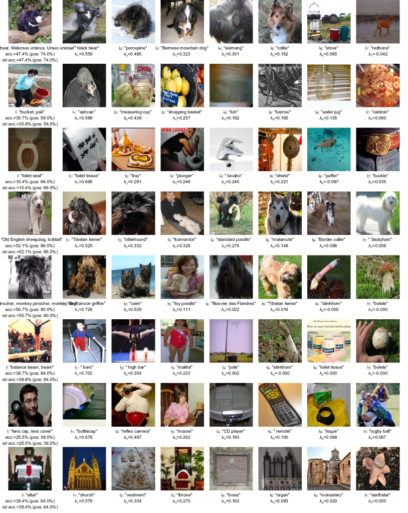
Figure A5: Results from ResNet-18, where ‘acc.’ and ‘ori acc.’ denote the classification accuracies on the ImageNet validation set, while ‘pos: xx%’ is the accuracy on positive samples only.

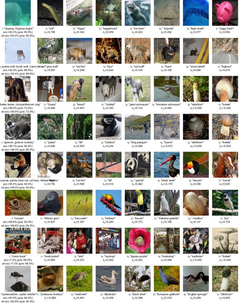
Figure A6: Results from ResNet-50, where ‘acc.’ and ‘ori acc.’ denote the classification accuracies on the ImageNet validation set, while ‘pos: xx%’ is the accuracy on positive samples only.

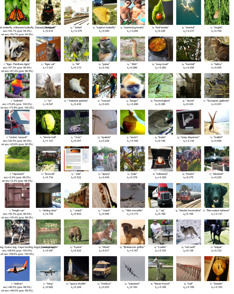
Figure A7: Results from ViT-S, where ‘acc.’ and ‘ori acc.’ denote the classification accuracies on the ImageNet validation set, while ‘pos: xx%’ is the accuracy on positive samples only.

n

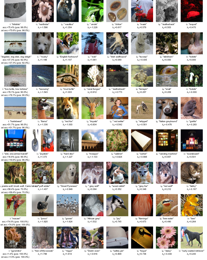
Figure A8: Results from Swin-T, where ‘acc.’ and ‘ori acc.’ denote the classification accuracies on the ImageNet validation set, while ‘pos: xx%’ is the accuracy on positive samples only.

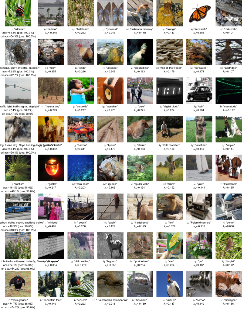
Figure A9: Results from ResNet-50$\to$Swin-T, where ‘acc.’ and ‘ori acc.’ denote the classification accuracies on the ImageNet validation set, while ‘pos: xx%’ is the accuracy on positive samples only.

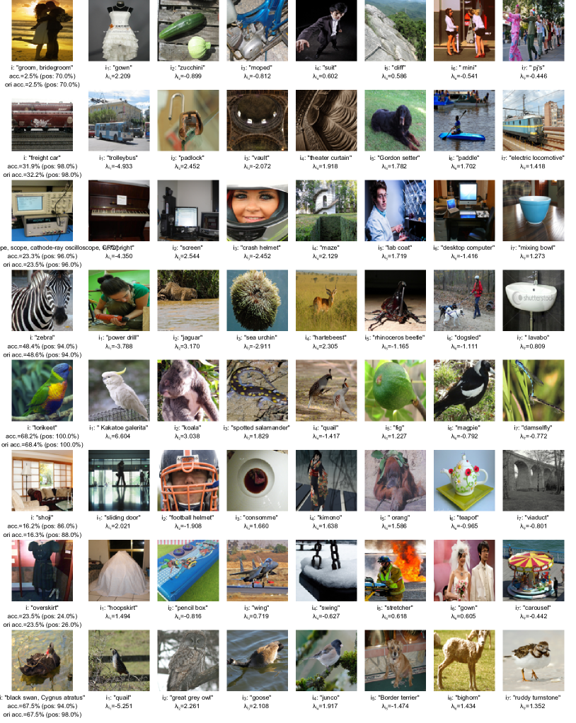
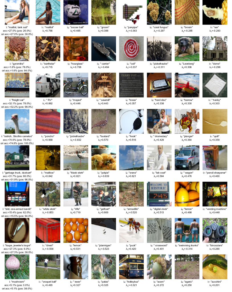
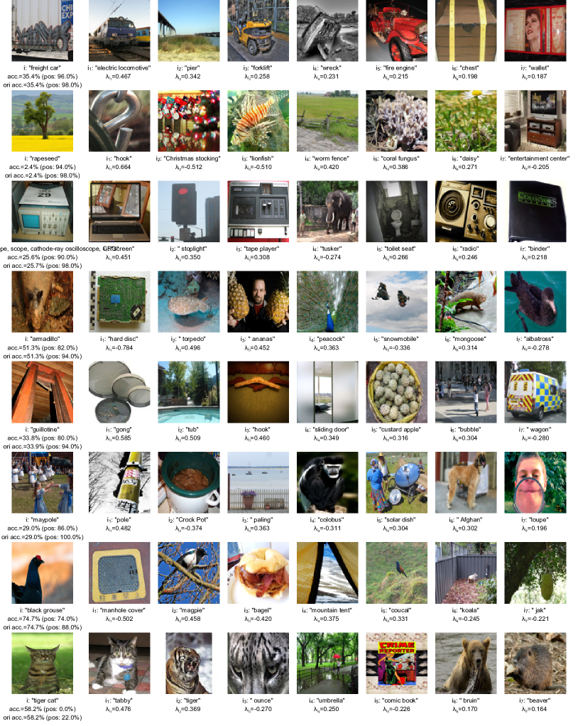
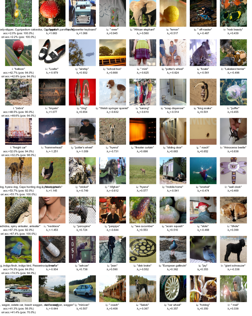
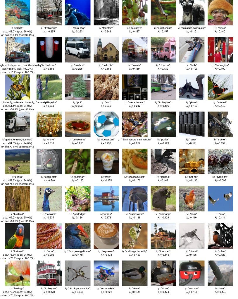
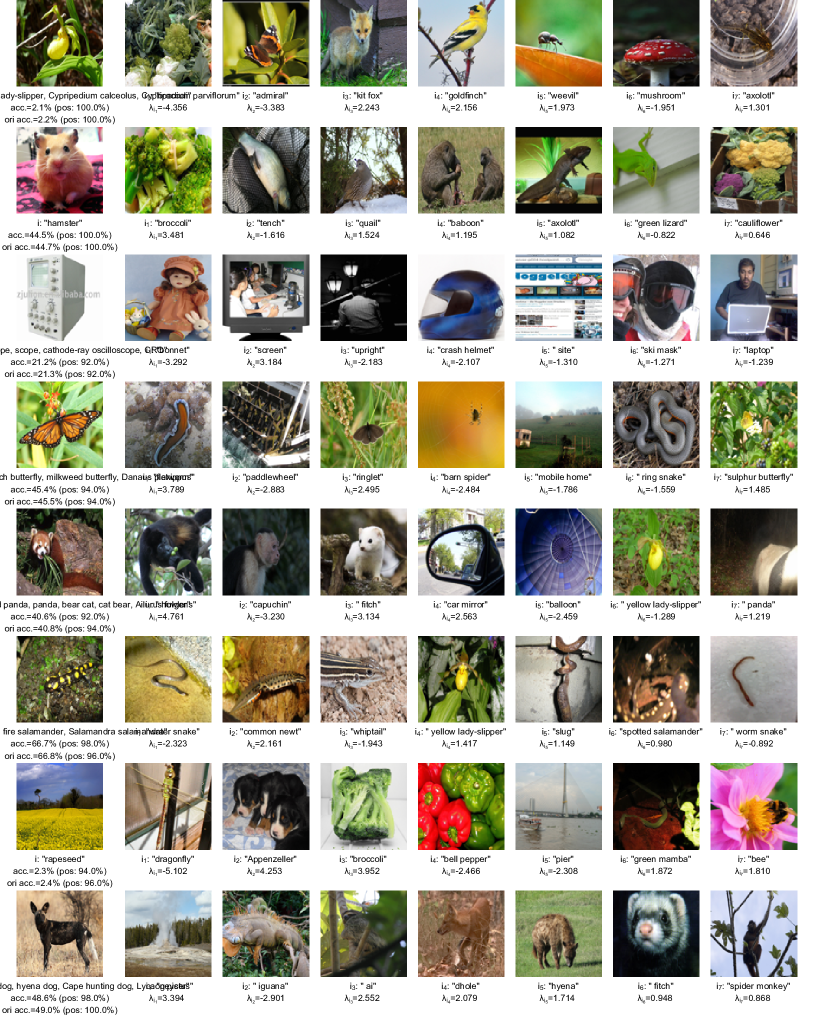
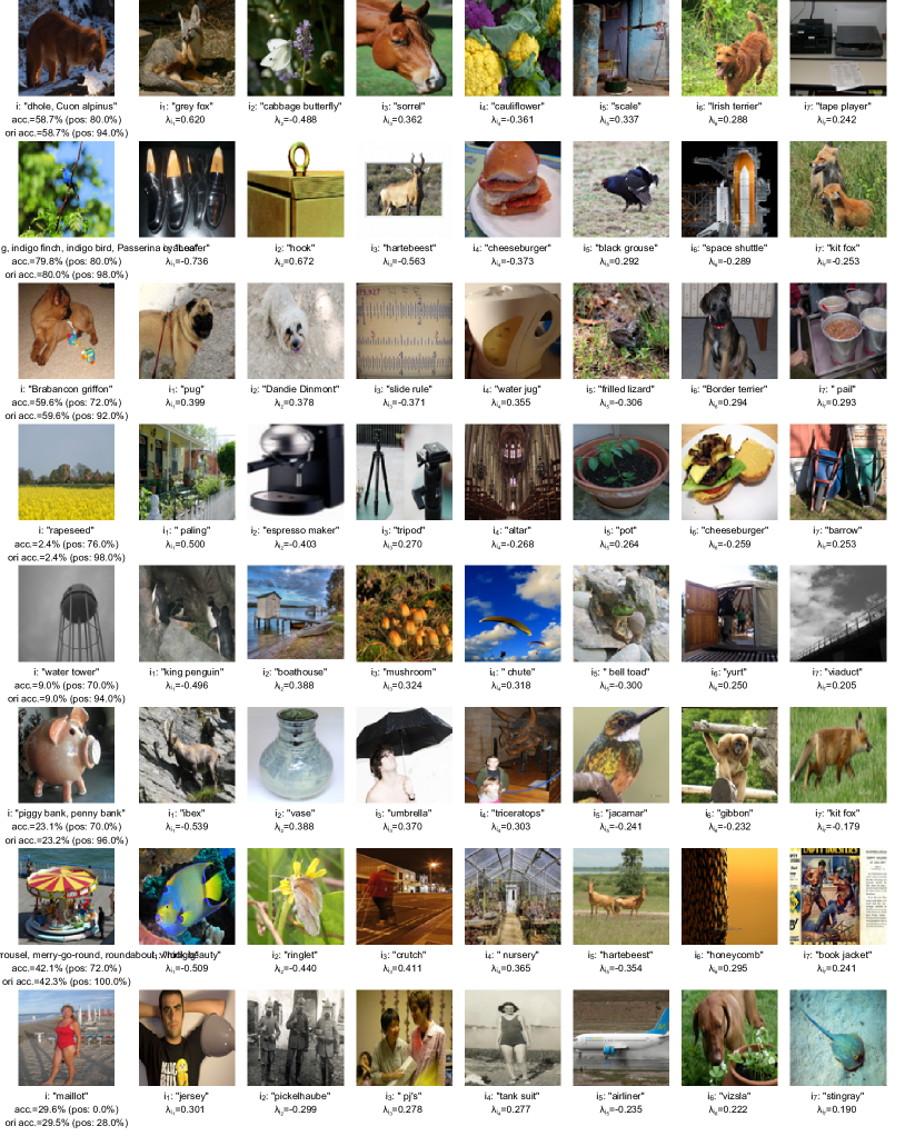
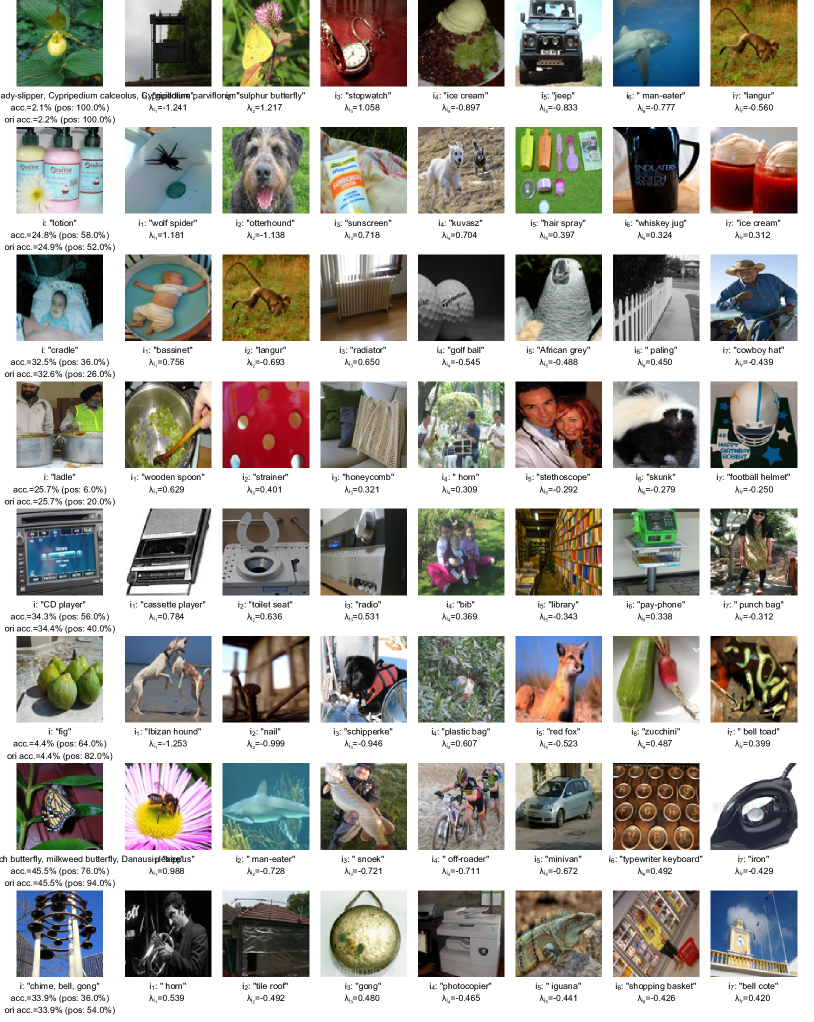
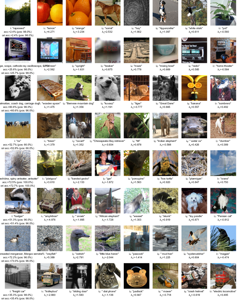
Figure A10: Results from Swin-T$\to$ResNet-50, where ‘acc.’ and ‘ori acc.’ denote the classification accuracies on the ImageNet validation set, while ‘pos: xx%’ is the accuracy on positive samples only.

Figure A11: Results from ResNet-50$\to$ResNet-18, where ‘acc.’ and ‘ori acc.’ denote the classification accuracies on the ImageNet validation set, while ‘pos: xx%’ is the accuracy on positive samples only.

Figure A12: Results from ResNet-18$\to$ResNet-50, where ‘acc.’ and ‘ori acc.’ denote the classification accuracies on the ImageNet validation set, while ‘pos: xx%’ is the accuracy on positive samples only.

Figure A13: Results from ResNet-50$\to$ViT-S, where ‘acc.’ and ‘ori acc.’ denote the classification accuracies on the ImageNet validation set, while ‘pos: xx%’ is the accuracy on positive samples only.

Figure A14: Results from ViT-S$\to$ResNet-50, where ‘acc.’ and ‘ori acc.’ denote the classification accuracies on the ImageNet validation set, while ‘pos: xx%’ is the accuracy on positive samples only.

Figure A15: Results from ResNet-18$\to$Swin-T, where ‘acc.’ and ‘ori acc.’ denote the classification accuracies on the ImageNet validation set, while ‘pos: xx%’ is the accuracy on positive samples only.

Figure A16: Results from Swin-T$\to$ResNet-18, where ‘acc.’ and ‘ori acc.’ denote the classification accuracies on the ImageNet validation set, while ‘pos: xx%’ is the accuracy on positive samples only.

Figure A17: Results from ResNet-50$\to$ViT-S, where ‘acc.’ and ‘ori acc.’ denote the classification accuracies on the ImageNet validation set, while ‘pos: xx%’ is the accuracy on positive samples only.

Figure A18: Results from ViT-S$\to$ResNet-18, where ‘acc.’ and ‘ori acc.’ denote the classification accuracies on the ImageNet validation set, while ‘pos: xx%’ is the accuracy on positive samples only.

Figure A19: Results from Swin-T$\to$ViT-S, where ‘acc.’ and ‘ori acc.’ denote the classification accuracies on the ImageNet validation set, while ‘pos: xx%’ is the accuracy on positive samples only.

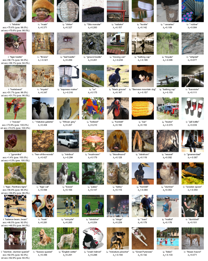
Figure A20: Results from ViT-S$\to$Swin-T, where ‘acc.’ and ‘ori acc.’ denote the classification accuracies on the ImageNet validation set, while ‘pos: xx%’ is the accuracy on positive samples only.

References

[1]
Yoshua Bengio, Aaron Courville, and Pascal Vincent.
Representation learning: A review and new perspectives.
IEEE Transactions on Pattern Analysis and Machine Intelligence
(TPAMI), 35(8):1798–1828, 2013.
[2]
Kendrick Boyd, Kevin H Eng, and C David Page.
Area under the precision-recall curve: point estimates and confidence
intervals.
In Joint European Conference on Machine Learning and Knowledge
Discovery in Databases, pages 451–466, 2013.
[3]
Stephen Boyd, Stephen P Boyd, and Lieven Vandenberghe.
Convex optimization.
Cambridge university press, 2004.
[4]
Peter Bühlmann and Sara Van De Geer.
Statistics for high-dimensional data: methods, theory and
applications.
Springer Science & Business Media, 2011.
[5]
Francisco M Castro, Manuel J Marín-Jiménez, Nicolás Guil, Cordelia
Schmid, and Karteek Alahari.
End-to-end incremental learning.
In Proceedings of the European Conference on Computer Vision
(ECCV), pages 233–248, 2018.
[6]
Xi Chen, Xiao Wang, Soravit Changpinyo, AJ Piergiovanni, Piotr Padlewski,
Daniel Salz, Sebastian Goodman, Adam Grycner, Basil Mustafa, Lucas Beyer,
et al.
Pali: A jointly-scaled multilingual language-image model.
arXiv preprint arXiv:2209.06794, 2022.
[7]
Jia Deng, Wei Dong, Richard Socher, Li-Jia Li, Kai Li, and Li Fei-Fei.
Imagenet: A large-scale hierarchical image database.
In Proceedings of the IEEE/CVF Conference on Computer Vision and
Pattern Recognition (CVPR), pages 248–255, 2009.
[8]
Alexey Dosovitskiy, Lucas Beyer, Alexander Kolesnikov, Dirk Weissenborn,
Xiaohua Zhai, Thomas Unterthiner, Mostafa Dehghani, Matthias Minderer, Georg
Heigold, Sylvain Gelly, et al.
An image is worth 16x16 words: Transformers for image recognition at
scale.
arXiv preprint arXiv:2010.11929, 2020.
[9]
Ruili Feng, Kecheng Zheng, Yukun Huang, Deli Zhao, Michael Jordan, and
Zheng-Jun Zha.
Rank diminishing in deep neural networks.
arXiv preprint arXiv:2206.06072, 2022.
[10]
Kaiming He, Xiangyu Zhang, Shaoqing Ren, and Jian Sun.
Deep residual learning for image recognition.
In Proceedings of the IEEE/CVF Conference on Computer Vision and
Pattern Recognition (CVPR), pages 770–778, 2016.
[11]
Dan Hendrycks, Kevin Zhao, Steven Basart, Jacob Steinhardt, and Dawn Song.
Natural adversarial examples.
In Proceedings of the IEEE/CVF Conference on Computer Vision and
Pattern Recognition (CVPR), pages 15262–15271, 2021.
[12]
Alex Krizhevsky, Geoffrey Hinton, et al.
Learning multiple layers of features from tiny images.
2009.
[13]
Alex Krizhevsky, Ilya Sutskever, and Geoffrey E Hinton.
Imagenet classification with deep convolutional neural networks.
Communications of the ACM, 60(6):84–90, 2017.
[14]
Ze Liu, Yutong Lin, Yue Cao, Han Hu, Yixuan Wei, Zheng Zhang, Stephen Lin, and
Baining Guo.
Swin transformer: Hierarchical vision transformer using shifted
windows.
In Proceedings of the IEEE/CVF International Conference on
Computer Vision (ICCV), pages 10012–10022, 2021.
[15]
Sudhanshu Mittal, Silvio Galesso, and Thomas Brox.
Essentials for class incremental learning.
In Proceedings of the IEEE/CVF Conference on Computer Vision and
Pattern Recognition (CVPR), pages 3513–3522, 2021.
[16]
Sinno Jialin Pan and Qiang Yang.
A survey on transfer learning.
IEEE Transactions on Knowledge and Data Engineering (TKDE),
22(10):1345–1359, 2009.
[17]
F. Pedregosa, G. Varoquaux, A. Gramfort, V. Michel, B. Thirion, O. Grisel, M.
Blondel, P. Prettenhofer, R. Weiss, V. Dubourg, J. Vanderplas, A. Passos, D.
Cournapeau, M. Brucher, M. Perrot, and E. Duchesnay.
Scikit-learn: Machine learning in Python.
Journal of Machine Learning Research, 12:2825–2830, 2011.
[18]
Ramprasaath R Selvaraju, Michael Cogswell, Abhishek Das, Ramakrishna Vedantam,
Devi Parikh, and Dhruv Batra.
Grad-cam: Visual explanations from deep networks via gradient-based
localization.
In Proceedings of the IEEE/CVF International Conference on
Computer Vision (ICCV), pages 618–626, 2017.
[19]
Robert Tibshirani.
Regression shrinkage and selection via the lasso.
Journal of the Royal Statistical Society: Series B
(Methodological), 58(1):267–288, 1996.
[20]
Ryan J Tibshirani and Jonathan Taylor.
The solution path of the generalized lasso.
The Annals of Statistics, 39(3):1335–1371, 2011.
[21]
Zhengzhong Tu, Hossein Talebi, Han Zhang, Feng Yang, Peyman Milanfar, Alan
Bovik, and Yinxiao Li.
Maxvit: Multi-axis vision transformer.
arXiv preprint arXiv:2204.01697, 2022.
[22]
Mei Wang and Weihong Deng.
Deep visual domain adaptation: A survey.
Neurocomputing, 312:135–153, 2018.
[23]
Karl Weiss, Taghi M Khoshgoftaar, and DingDing Wang.
A survey of transfer learning.
Journal of Big Data, 3(1):1–40, 2016.
[24]
Mitchell Wortsman, Gabriel Ilharco, Samir Ya Gadre, Rebecca Roelofs, Raphael
Gontijo-Lopes, Ari S Morcos, Hongseok Namkoong, Ali Farhadi, Yair Carmon,
Simon Kornblith, et al.
Model soups: averaging weights of multiple fine-tuned models improves
accuracy without increasing inference time.
In Proceedings of the International Conference on Machine
Learning (ICML), pages 23965–23998, 2022.
[25]
Yue Wu, Yinpeng Chen, Lijuan Wang, Yuancheng Ye, Zicheng Liu, Yandong Guo, and
Yun Fu.
Large scale incremental learning.
In Proceedings of the IEEE/CVF Conference on Computer Vision and
Pattern Recognition (CVPR), pages 374–382, 2019.
[26]
Jiahui Yu, Zirui Wang, Vijay Vasudevan, Legg Yeung, Mojtaba Seyedhosseini, and
Yonghui Wu.
Coca: Contrastive captioners are image-text foundation models.
arXiv preprint arXiv:2205.01917, 2022.
[27]
Bolei Zhou, Aditya Khosla, Agata Lapedriza, Aude Oliva, and Antonio Torralba.
Learning deep features for discriminative localization.
In Proceedings of the IEEE/CVF Conference on Computer Vision and
Pattern Recognition (CVPR), pages 2921–2929, 2016.