Compact object mergers: exploring uncertainties from stellar and binary evolution with sevn

Abstract

Population-synthesis codes are an unique tool to explore the parameter space of massive binary star evolution and binary compact object (BCO) formation. Most population-synthesis codes are based on the same stellar evolution model, limiting our ability to explore the main uncertainties. Here, we present the new version of the code sevn, which overcomes this issue by interpolating the main stellar properties from a set of pre-computed evolutionary tracks. We describe the new interpolation and adaptive time-step algorithms of sevn, and the main upgrades on single and binary evolution. With sevn, we evolved $1.2\times 10^{9}$ binaries in the metallicity range $0.0001\leq Z\leq 0.03$, exploring a number of models for electron-capture, core-collapse and pair-instability supernovae, different assumptions for common envelope, stability of mass transfer, quasi-homogeneous evolution and stellar tides. We find that stellar evolution has a dramatic impact on the formation of single and binary compact objects. Just by slightly changing the overshooting parameter ($\lambda_{\rm ov}=0.4$, 0.5) and the pair-instability model, the maximum mass of a black hole can vary from $\approx{60}$ to $\approx{100}\ \mbox{M${}_{\odot}$}$. Furthermore, the formation channels of BCOs and the merger efficiency we obtain with sevn show significant differences with respect to the results of other population-synthesis codes, even when the same binary-evolution parameters are used. For example, the main traditional formation channel of BCOs is strongly suppressed in our models: at high metallicity ($Z\gtrsim{0.01}$) only $<20$% of the merging binary black holes and binary neutron stars form via this channel, while other authors found fractions $>70$%.

1 Introduction

Since the first detection in September 2015, the LIGO–Virgo–KAGRA collaboration (LVK) has reported 90 binary compact object (BCO) merger candidates, most of them binary black holes (BBHs, Abbott et al. 2016b, a, c, 2019a, 2019b, 2021c, 2021d, 2021a, 2021b). The LVK data have confirmed that BBHs exist, and probed a mass spectrum of black holes (BHs) ranging from a few to $\sim{200}$ M_⊙ (Abbott et al., 2016c, 2019b, 2021d, 2023). This result has revolutionised our knowledge of stellar-sized BHs, complementing electromagnetic (e.g., Özel et al., 2010; Farr et al., 2011) and microlensing data (e.g., Wyrzykowski et al., 2016). Some peculiar LVK events even challenge current evolutionary models, indicating the existence of compact objects inside the claimed lower (e.g., Abbott et al., 2020c) and upper mass gap (e.g., Abbott et al., 2020a, d, 2021a). Finally, the first and so far only multi-messenger detection of a binary neutron star (BNS) merger (e.g., Abbott et al., 2017a, b) has confirmed the association of kilonovae and short gamma-ray bursts with mergers of neutron stars (NSs), paving the ground for a novel synergy between gravitational-wave (GW) scientists and astronomers.

This wealth of new data triggered an intense debate on the formation channels of BCOs (see, e.g., Mandel & Farmer 2022 and Mapelli 2021 for two recent reviews on this topic). One of the main problems of the models is the size of the parameter space: even if we restrict our attention to BCO formation via binary evolution, countless assumptions about the evolution of massive binary stars can have a sizeable impact on the final BCO properties. Hence, numerical models used to probe BCO populations need to be computationally fast, while achieving the highest possible level of accuracy and flexibility. Binary population synthesis codes are certainly the fastest approach to model binary star evolution, from the zero-age main sequence (ZAMS) to the final fate. For example, the famous bse code (Hurley et al., 2000, 2002), which is the common ancestor of most binary population synthesis codes, evolves $\mathcal{O}(10^{6})$ binary stars in a couple of hours on a single CPU core. For comparison, a modern stellar evolution code requires $\mathcal{O}(10-100)$ CPU hours to integrate the evolution of an individual binary star. The speed of binary population synthesis codes is essential not only to model the parameter space of massive binary star evolution, but also to guarantee that they can be interfaced with dynamical codes to study the dynamical formation of BCOs in dense stellar clusters (e.g., Banerjee et al., 2010; Tanikawa, 2013; Mapelli et al., 2013; Ziosi et al., 2014; Rodriguez et al., 2015, 2016; Mapelli, 2016; Banerjee, 2017, 2018; Rastello et al., 2019; Banerjee et al., 2020; Banerjee, 2021; Di Carlo et al., 2019; Di Carlo et al., 2020b, 2021; Kremer et al., 2020b, a; Rastello et al., 2020; Ye et al., 2022; Wang, 2020; Rastello et al., 2021; Wang et al., 2022).

A large number of binary population synthesis codes have been developed across the years and most of them have been used to study the formation of BCOs, e.g., binary_c (Izzard et al., 2004, 2006, 2009, 2018), bpass (Eldridge et al., 2017), the Brussels code (Vanbeveren et al., 1998; De Donder & Vanbeveren, 2004; Mennekens & Vanbeveren, 2014), bse-LevelC (Kamlah et al., 2022), combine (Kruckow et al., 2018), compas (Riley et al., 2022), cosmic (Breivik et al., 2020), IBis (Tutukov & Yungelson, 1996), metisse (Agrawal et al., 2020), mobse (Mapelli et al., 2017; Giacobbo et al., 2018), posydon (Fragos et al., 2023), the Scenario Machine (Lipunov et al., 1996, 2009), SeBa (Portegies Zwart & Verbunt, 1996; Toonen et al., 2012), sevn (Spera et al., 2019; Mapelli et al., 2020), and startrack (Belczynski et al., 2002; Belczynski et al., 2008).

While all of them are independent codes, most of them rely on the same model of stellar evolution: the accurate and computationally efficient fitting formulas developed by Hurley et al. (2000), based on the stellar tracks by Pols et al. (1998). These fitting formulas express the main stellar evolution properties (e.g., photospheric radius, core mass, core radius, luminosity) as a function of stellar age, mass ($M$), and metallicity ($Z$, mass fraction of elements heavier than helium). The results of binary population synthesis codes adopting such fitting formulas can differ by the way they model stellar winds, compact-remnant formation and binary evolution, but rely on the same stellar evolution model. This implies that they can probe only a small portion of the parameter space, which is the physics encoded in the original tracks by Pols et al. (1998). Stellar evolution models have dramatically changed since 1998, including, e.g., new calibrations for core overshooting (e.g., Claret & Torres, 2018; Costa et al., 2019), updated networks of nuclear reactions (e.g., Cyburt et al., 2010; Sallaska et al., 2013), updated opacity tables (e.g., Marigo & Aringer, 2009; Poutanen, 2017), and new sets of stellar tracks with rotation (e.g., Brott et al., 2011; Chieffi & Limongi, 2013; Georgy et al., 2013; Choi et al., 2016; Nguyen et al., 2022). Moreover, the newest stellar evolution models probe a much wider mass and metallicity range (e.g., Spera & Mapelli, 2017) than the range encompassed by Hurley et al. (2000) fitting formulas ($0.5\leq{}M/{\rm M}_{\odot}\leq{}50$, $0.0001\leq{}Z\leq{}0.03$).

Driven by the need to include up-to-date stellar evolution and a wider range of masses and metallicities, several binary population synthesis codes adopt an alternative strategy with respect to Hurley et al. (2000) fitting formulas. bpass (Eldridge et al., 2008; Eldridge & Stanway, 2016; Eldridge et al., 2017) integrates stellar evolution on-the-fly with a custom version of the Cambridge stars stellar evolution code (Eggleton, 1971; Pols et al., 1995; Eldridge & Tout, 2004). To limit the computational time, the primary star (i.e., the most massive star in the binary system) is first evolved with stars, while the secondary is evolved with the fitting formulas by Hurley et al. (2000). After the evolution of the primary star is complete, the evolution of the secondary is re-integrated with stars.

combine (Kruckow et al., 2018), metisse (Agrawal et al., 2020), posydon (Fragos et al., 2023) and sevn (Spera et al., 2015; Spera & Mapelli, 2017; Spera et al., 2019; Mapelli et al., 2020) share the same approach to stellar evolution: they include an algorithm that interpolates the main stellar-evolution properties (mass, radius, core mass and radius, luminosity, etc as a function of time and metallicity) from a number of pre-computed tables. The main advantage is that the interpolation algorithm is more flexible than the fitting formulas: it is sufficient to generate new tables, in order to update the stellar-evolution model. Furthermore, this approach allows to easily compare different stellar-evolution models encoding different physics (e.g., different stellar-evolution codes, different overshooting models, different convection criteria). Among the aforementioned codes, posydon is the only one that includes tables of binary star evolution, run with the code mesa (Paxton et al., 2011; Paxton et al., 2013, 2015, 2018), while the others are based on single star evolution tables. Including binary-evolution in the look-up tables has the advantage of encoding the response of each star to interactions between binary components. This level of model sophistication comes with increased data size: the look-up tables for a given metallicity weigh $\mathcal{O}(100)$ MB for single star evolution, and $\mathcal{O}(10)$ GB for binary evolution, respectively. Overall, binary population synthesis codes based on look-up tables are a powerful tool to probe the parameter space of BCO formation with up-to-date stellar evolution.

Here, we present a new version of our binary population synthesis code sevn, and use it to explore some of the main uncertainties in BCO formation springing from stellar and binary evolution. This paper is organised as follows. Section 2 describes the main features of sevn. In Section 3, we describe the stellar evolution models used in this work, our initial conditions, and the main parameters/assumptions tested with our simulations. Section 4 shows the properties of BCOs formed in our simulations, their mass spectrum, merger efficiency, and local merger rate density. In Section 5, we discuss our results and their possible caveats. Finally, Section 6 is a summary of our main results.

2 Description of sevn

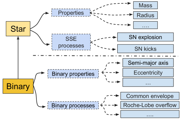
Figure 1: In sevn, single stars, binary systems, properties and processes are represented with C++ classes. Single stars are characterised by their properties (mass, radius,…) and single stellar evolution processes (supernova explosion type and natal kicks). Binary stars are characterised by their properties (semi-major axis, eccentricity,..), binary-evolution processes (mass transfer by winds, Roche-lobe overflow, CE, tides,..), and by the two stars component of the binary system.

sevn (Stellar EVolution for $N$-body) is a rapid binary population synthesis code, which calculates stellar evolution by interpolating pre-computed sets of stellar tracks (Spera et al., 2015; Spera & Mapelli, 2017; Spera et al., 2019; Mapelli et al., 2020). Binary evolution is implemented by means of analytic and semi-analytic prescriptions. The main advantage of this strategy is that it makes the implementation more general and flexible: the stellar evolution models adopted in sevn can easily be changed or updated just by loading a new set of look-up tables. sevn allows to choose the stellar tables at runtime, without modifying the internal structure of the code or even recompiling it.

The current version of sevn is grounded on the same basic concepts developed for the previous versions (see, e.g., Spera & Mapelli, 2017; Spera et al., 2019), but the code has been completely refactored, improved in many aspects (e.g. time step, modularity), extended with new functionalities/options, and updated with the latest parsec stellar evolution tracks (Bressan et al., 2012; Chen et al., 2015; Costa et al., 2021; Nguyen et al., 2022). sevn is written entirely in C++ (without external dependencies) following the object-oriented programming paradigm. sevn exploits the CPU-parallelisation through OpenMP. Figure 1 shows a schematic representation of the basic sevn components and their relations.

In the following sections, we describe the main features and options of sevn focusing on the new prescriptions used in this work. Additional information about sevn can be found in Appendix A. sevn is publicly available at this link; the version used in this work is the release Iorio22.

2.1 Single star evolution

In the following sections, we describe the main ingredients used in sevn to integrate stellar evolution from the ZAMS to the formation of the compact remnant. Additional information can be found in Appendix A.

2.1.1 Stellar evolution tables

sevn tables
Table	Units	Type	Interpolation
Time	Myr	M	R
Phase$\dagger$	Myr$\dagger$	M	R
Mass	M⊙	M	LIN
Luminosity	L⊙	M	LOG
Radius	R⊙	M	LOG
He-core mass	M⊙	M	LIN
CO-core mass	M⊙	M	LIN
He-core Radius	R⊙	O	LIN
CO-core Radius	R⊙	O	LIN
Stellar inertia$\ddagger$	$\mbox{M${}_{\odot}$}{}\mbox{R${}_{\odot}$}^{2}$	O	LOG
Envelope binding energy$\ddagger$	$\mbox{M${}_{\odot}$}{}^{2}\mbox{R${}_{\odot}$}^{-1}(G^{-1})*$	O	LOG
Surface abundances $\ddagger$	mass fraction	O	LIN
(H,He,C,N,O)
Convective envelope
mass	normalised to star mass	O	LIN
depth	normalised to star radius	O	LIN
turnover time	yr	O	LIN

Table 1: Summary of the stellar evolution tables used in sevn. The first column reports the property stored in the table, the second column its units and the third column specifies if a table is mandatory (M) or optional (O). sevn includes analytic recipes to replace the optional tables if they are not available (Appendix A.1). The fourth column indicates the type of weights used by sevn during the property interpolation: rational (R), linear (LIN), log (LOG), see Section 2.1.4. $\dagger$ The phase table reports the starting time of each sevn phase (Table 2). $\ddagger$Not included in the stellar tracks used in this work (Section 3.1). The envelope binding energy is normalised over the gravitational constant $G$ (assumed in solar units and years).

The sevn stellar-evolution tables contain the evolution of the properties of a set of stellar tracks defined by their initial mass $M_{\mathrm{ZAMS}}$ and metallicity $Z$. sevn requires, as input, two sets of tables: one for stars that start their life from the hydrogen main sequence (MS; hereafter, H stars), the other for stars that are H depleted (hereafter, pure-He stars). Unlike bse, sevn assumes that the stellar models already include wind mass loss.

Table 1 summarises the tables available in sevn. Each stellar-evolution model comprises (at least) seven tables grouped by metallicity. The tables for each metallicity are stored in different directories. Each table refers to a given stellar property. There are seven mandatory tables corresponding to the main stellar properties: time, total stellar mass, He-core mass, CO-core mass, stellar radius, bolometric luminosity, and the stellar phase (Section 2.1.3). Each row in the tables refers to a star with a given $M_{\mathrm{ZAMS}}$ and $Z$, each column stores the value of the property at the time correspondent to the same row and column in the time table. The first column of each row in the mass table identifies the $M_{\mathrm{ZAMS}}$ of the star. The stellar-phase table contains the starting time for the stellar phases (Section 2.1.3). The end of the evolution (i.e., the stellar lifetime) is not reported in the phase table, rather sevn implicitly assumes it is equal to the last value reported in the time tables.

Additional properties such as the radii of the He and CO cores, the envelope binding energy, and the properties of the convective envelope (mass, extension, eddy turnover timescale) are optional. If such tables are not provided (or disabled by the user), sevn estimates these properties using alternative analytic approximations (Appendix A.1). These tables are not mandatory because they contain information that is not available in most stellar-evolution tracks, but they are essential to properly model several evolution processes. For example, the properties of the convective envelope allow a more physical identification of the evolutionary phase and can be used to estimate the stability of mass transfer (Section 2.3.2), in addition they also play an important role in setting the efficiency of stellar tides (Section 2.3.2). The modular structure of sevn makes it possible to easily introduce new tables to follow the evolution of additional stellar properties. sevn does not assume a specific definition for the mass and radius of the He and CO cores. The estimate of such properties depends on the adopted stellar evolution models and/or on the user choice in the production of the sevn tables (Section 3.1).

2.1.2 TrackCruncher

The most important requirement of the tables is that they must capture all the main features of the stellar tracks they are generated from, but at the same time they must be as small as possible (up to a few MB each), to make the interpolation fast and to reduce the memory cost. In order to satisfy these requirements, we developed the code TrackCruncher, which we use to efficiently generate the tables for sevn. This code extracts the properties to store in the sevn tables from a set of stellar tracks, while estimating the starting time of the sevn phases (see Section 2.1.3 and Appendix B). In addition, TrackCruncher decides which time-steps of the original tracks can be omitted in the final tables, in order to reduce the table size. In particular, we store in the final tables only the time-steps of the original tracks that guarantee errors smaller than 2% when we perform a linear interpolation to model the evolution of the stellar properties (Section 2.1.4). This track under-sampling reduces significantly the size of the tables, from $\mathcal{O}$(1 GB) to $\mathcal{O}$(10 MB). For example, the complete set of tables for H stars (pure-He stars) used in this work (see Section 3.1) occupies only ${\sim}30$ MB (${\sim}10$ MB), while the original tracks consume ${\sim}5$ GB (${\sim}6$ GB) of disc space. This procedure significantly reduces both the storage and runtime memory footprint of sevn; moreover it speeds up single stellar evolution computation (see Section 2.4.1).

TrackCruncher is publicly available at this link. It is optimized to process the outputs of parsec (Bressan et al., 2012), franec (Limongi & Chieffi, 2018), and the mist stellar tracks (Choi et al., 2016), but can easily be extended to process the output of other stellar evolution codes. TrackCruncher can also be used as a tool to compress and reduce the memory size of stellar tracks.

The specific description of the stellar tables used in this work can be found in Section 3.1 and Appendix B.

2.1.3 Stellar phases

sevn Phase	Phase ID	sevn Remnant subphase	Remnant ID	bse stellar-type equivalent
Pre-main sequence (PMS)	0	–	0	not available
Main sequence (MS)	1	–	0	1 if $f_{\mathrm{conv}}^{\dagger}<0.8$, else 0
Terminal-age main sequence (TAMS)	2	–	0	$2$ if $f_{\mathrm{conv}}^{\dagger}<0.33$, else $3$
Shell H burning (SHB)	3	–	0
Core He burning (CHeB)	4	–	0	7 if WR‡, else 4
Terminal-age core He burning (TCHeB)	5	–	0	7 if WR‡, else: 4 if $f_{\mathrm{conv}}^{\dagger}<0.33$, else 5
Shell He burning (SHeB)	6	–	0	8 if WR‡, else: 4 if $f_{\mathrm{conv}}^{\dagger}<0.33$ else 5
Remnant	7	He white dwarf (HeWD)	1	10
		CO white dwarf (COWD)	2	11
		ONe white dwarf (ONeWD)	3	12
		neutron star formed via electron capture (ECNS)	4	13
		neutron star formed via core collapse (CCNS)	5	13
		black hole (BH)	6	14
		no compact remnant (Empty)	-1	15

Table 2: sevn stellar evolutionary phases (Column 0), identifiers (Column 1) and remnant types (Column 2). Column 3 shows the correspondence to Hurley et al. (2000, 2002) stellar types: 0, low-mass main sequence (MS); 1, main sequence (MS); 2, Hertzsprung-gap (HG); 3, first giant branch (GB); 4, core-helium burning (CHeB); 5, early asymptotic giant branch (EAGB); 7, naked-helium MS (HeMS); 8, naked-helium HG (HeHG). The bse stellar types 6 (thermally pulsating AGB) and 9 (naked-helium giant branch) do not have a correspondent sevn phase. ECNS and CCNS are NSs produced by electron capture and core collapse supernovae, respectively (Section 2.2). $\dagger$ $f_{\mathrm{conv}}$ is the mass fraction of the convective envelope over the total envelope mass (total mass in case of MS stars), $\ddagger$ WR indicates Wolf-Rayet (WR) stars, i.e., stars which have a He core mass larger than 97.9% of the total mass. See Section 2.1.3 for additional details.

Spera et al. (2019) found that the interpolation of stellar evolution properties significantly improves if we use the percentage of life of a star instead of the absolute value of the time (Section 2.1.4). In order to further refine the interpolation, they estimate the percentage of life in three stellar macro-phases: i) the H phase, in which the star has not developed a He core yet; ii) the He phase, when the star has a He core but not a CO core; iii) the CO phase, when the star has a CO core.

In the current version of sevn, we refine the definition of macro-phases in Spera et al. (2019) by dividing stellar evolution in seven physically motivated phases. The phase from time 0 to the ignition of hydrogen burning in the core is the pre-main sequence (PMS, phase id $=0$). During core-hydrogen burning, the star is in the main sequence (MS, phase id $=1$) phase until its He core starts to grow (He-core mass $>0$) and the star enters the terminal-age MS (TAMS, phase id $=2$). The next phase, shell H burning (SHB, phase id $=3$), starts when the hydrogen in the core has been completely exhausted and the star is burning hydrogen in a thin shell around the He core. At the ignition of core helium burning, the star enters the core He burning phase (CHeB, phase id $=4$), which is followed by the terminal-age core He burning (TCHeB, phase id $=5$, CO-core mass $>0$) and the shell He burning (SHeB, phase id $=6$). This last phase starts when helium has been completely exhausted in the core. The remnant phase (id $=7$) begins when the evolution time exceeds the star’s lifetime (see Section 2.1.1), and the star becomes a compact remnant (Section 2.2).

During its evolution, a star can be stripped of its hydrogen envelope either because of effective stellar winds or due to binary interactions. If the He-core mass is larger than 97.9% of the total stellar mass, sevn classifies the star as a Wolf-Rayet (WR) star (e.g., Bressan et al., 2012; Chen et al., 2015) and the star jumps to a new interpolating track on the pure-He tables (Section 2.4.3). In sevn, we do not use special phases for pure-He stars. The only difference with respect to hydrogen-rich stars is that a pure-He star does not go through phases 0–3, but rather starts its life from phase 4 (CHeB). Pure-He stars in sevn are equivalent to the stars defined as naked-He stars in other population synthesis codes derived from bse (Hurley et al., 2002).

During binary evolution, an evolved pure-He star can lose its He envelope leaving a naked-CO star. sevn does not have a dedicated phase for such objects, but they are considered compact remnant-like objects and evolve accordingly (Section 2.4.2). The conversion between sevn stellar phases and bse stellar types (Hurley et al., 2000) is summarised in Table 2.

2.1.4 Interpolation

We estimate the properties of each star at a given time via interpolation. The method implemented in this version of sevn is an improved version with respect to Spera et al. (2019). When a star is initialised, sevn assigns to it four interpolating tracks from the hydrogen or pure-He look-up tables. These four tracks have two different metallicities ($Z_{1}$, $Z_{2}$) and four different ZAMS masses ($M_{\rm ZAMS,1}$, $M_{\rm ZAMS,2}$, $M_{\rm ZAMS,3}$, $M_{\rm ZAMS,4}$, two per metallicity), chosen as $M_{\rm ZAMS,1/3}\leq M_{\rm ZAMS}<M_{\rm ZAMS,2/4}$ and $Z_{1}\leq Z<Z_{2}$ where $M_{\rm ZAMS}$ and $Z$ are the ZAMS mass and the metallicity of the star we want to calculate. In case $M_{\rm ZAMS}$ and/or $Z$ are equal to the maximum values in the tables, we use $M_{\rm ZAMS,1/3}<M_{\rm ZAMS}\leq M_{\rm ZAMS,2/4}$ and $Z_{1}<Z\leq Z_{2}$. A given interpolated property $W$ (e.g. the stellar mass) is estimated as follows.

$$W=\frac{Z_{2}-Z}{Z_{2}-Z_{1}}W_{\mathrm{Z,1}}+\frac{Z-Z_{1}}{Z_{2}-Z_{1}}W_{\mathrm{Z,2}},$$ (1)

where

$$\begin{split}W_{\mathrm{Z,1}}&=\beta_{1}W_{\mathrm{ZAMS,1}}+\beta_{2}W_{\mathrm{ZAMS,2}}\\ W_{\mathrm{Z,2}}&=\beta_{3}W_{\mathrm{ZAMS,3}}+\beta_{4}W_{\mathrm{ZAMS,4}}.\end{split}$$ (2)

In Eq. 2, $W_{\mathrm{ZAMS,i}}$ indicates the value of the property $W$ in the interpolating tracks with $M_{\mathrm{ZAMS,i}}$, and $\beta$ are interpolation weights. sevn includes three different interpolation weights:

• linear,

  $$\begin{split}\beta_{1/3}&=\frac{M_{\mathrm{ZAMS,2/4}}-M_{\mathrm{ZAMS}}}{M_{\mathrm{ZAMS,2/4}}-M_{\mathrm{ZAMS,1/3}}},\\ \ \beta_{2/4}&=\frac{M_{\mathrm{ZAMS}}-M_{\mathrm{ZAMS,1/3}}}{M_{\mathrm{ZAMS,2/4}}-M_{\mathrm{ZAMS,1/3}}};\end{split}$$ (3)

• logarithmic,

  $$\begin{split}\beta_{1/3}&=\frac{\log M_{\mathrm{ZAMS,2/4}}-\log M_{\mathrm{ZAMS}}}{\log M_{\mathrm{ZAMS,2/4}}-\log M_{\mathrm{ZAMS,1/3}}},\\ \ \beta_{2/4}&=\frac{\log M_{\mathrm{ZAMS}}-\log M_{\mathrm{ZAMS,1/3}}}{\log M_{\mathrm{ZAMS,2/4}}-\log M_{\mathrm{ZAMS,1/3}}};\end{split}$$ (4)

• rational,

  $$\begin{split}\beta_{1/3}&=\frac{M_{\mathrm{ZAMS,1/3}}\left(M_{\mathrm{ZAMS,2/4}}-M_{\mathrm{ZAMS}}\right)}{M_{\mathrm{ZAMS}}\left(M_{\mathrm{ZAMS,2/4}}-M_{\mathrm{ZAMS,1/3}}\right)},\\ \ \beta_{2/4}&=\frac{M_{\mathrm{ZAMS,2/4}}\left(M_{\mathrm{ZAMS}}-M_{\mathrm{ZAMS,1/3}}\right)}{M_{\mathrm{ZAMS}}\left(M_{\mathrm{ZAMS,2/4}}-M_{\mathrm{ZAMS,1/3}}\right)}.\end{split}$$ (5)

sevn uses logarithmic weights for the properties that are internally stored and interpolated in logarithmic scale, i.e., radius and luminosity. Spera et al. (2019) introduced the rational weights to improve the interpolation. In particular, we found that they drastically improve the estimate of the starting time of the stellar phases and the estimate of the star lifetime. For all the other properties, sevn uses linear weights (Table 1). Figure 2 clearly shows that the combination of different weights gives a much more reliable interpolation compared to using only linear weights.

When a star is initialised, sevn uses Eqs. 1 and 2 to set the starting times of the stellar phases, $t_{\mathrm{start,p}}$ (see, e.g., Section 2.1.3), where $W_{\mathrm{ZAMS,i}}$ represents the phase times from the phase table (Section 2.1.1). We interpolate the stellar lifetime in the same way, assuming that the last element in the sevn time table sets the stellar lifetime. For all the other properties, $W$ has to be estimated at a given time $t$. The corresponding $W_{\mathrm{ZAMS,i}}$ in the tables is not estimated at the same absolute time $t$, rather at the same percentage of life in the phase of the interpolated star (Section 2.1.3):

$$\Theta_{\mathrm{p}}=\frac{t-t_{\mathrm{start,p}}}{t_{\mathrm{start,p_{next}}}-t_{\mathrm{start,p}}},$$ (6)

where $t_{\mathrm{start,p}}$ indicates the starting time of the current phase $p$, and $t_{\mathrm{start,p_{\mathrm{next}}}}$ the starting time of next phase $p_{\mathrm{next}}$ (Table 2). Hence, sevn evaluates $W_{\mathrm{ZAMS,i}}$ at time

$$t_{\mathrm{i}}=t_{\mathrm{start,p,i}}+\Theta_{\mathrm{p}}\Delta_{\mathrm{p,i}},$$ (7)

where $t_{\mathrm{start,p,i}}$ and $\Delta_{\mathrm{p,i}}$ are the starting time and the time duration of the current phase for the interpolating track. In practice, sevn uses Eq. 6 to evaluate the times for each of the fourth interpolating tracks. Then, it estimates $W_{\mathrm{ZAMS,i}}$ in Eq. 2 by interpolating (linearly along the time) the values stored in the tables.

The division into phases guarantees that all the interpolating stars have the same internal structure (e.g., the presence or not of the core) improving significantly the interpolation method and reducing the interpolation errors to a few percent (Spera et al., 2019).

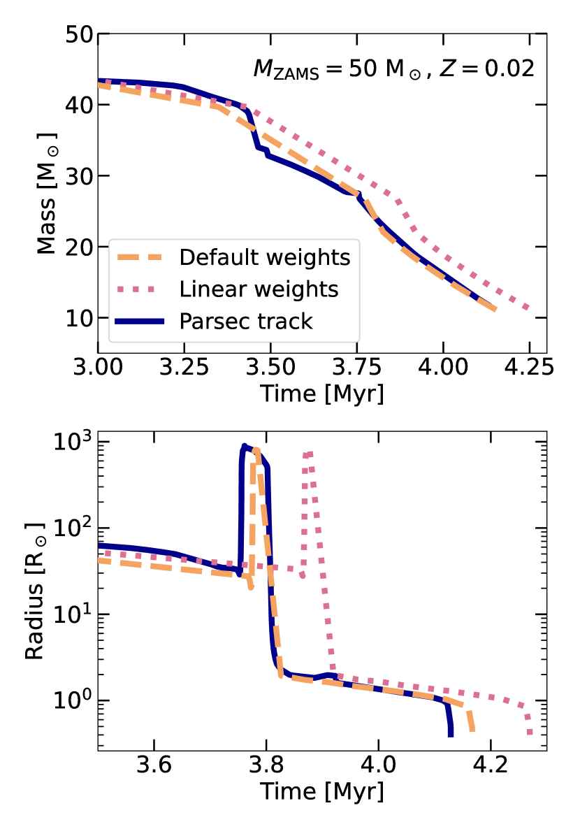
Figure 2: Time evolution of the mass (top) and radius (bottom) of a star with $M_{\mathrm{ZAMS}}=50\ \mbox{M${}_{\odot}$}$ and $Z=0.02$. The blue solid lines refer to a stellar track obtained with the code parsec  (Section 3.1), while the other lines show the sevn interpolation using pre-evolved tracks of two stars with $M_{\mathrm{ZAMS,1}}=40\ \mbox{M${}_{\odot}$}$, $M_{\mathrm{ZAMS,2}}=60\ \mbox{M${}_{\odot}$}$, and $Z=0.02$. We obtain the orange dashed line interpolation using the default weights: linear weights for the mass (Eq. 3), logarithmic weights for the radius (Eq. 4), and rational weights for the phase and time (Eq. 5). In contrast, we obtain the pink dotted curve using linear weights for all the properties.

2.1.5 Spin evolution

We model the evolution of stellar rotation through three properties: the fundamental quantity evolved in sevn is the spin angular momentum $J_{\mathrm{spin}}$, then we derive the angular velocity as $\Omega_{\mathrm{spin}}=J_{\mathrm{spin}}\,{}I^{-1}$ (where $I$ is the inertia), and estimate the spin $\omega_{\mathrm{spin}}$ as the ratio between $\Omega_{\mathrm{spin}}$ and the critical angular velocity $\Omega_{\mathrm{crit}}=\sqrt{G\,{}M\,{}(1.5\,{}R)^{-3}}$, where $G$ is the gravity constant, $M$ and $R$ are the stellar mass and radius. In this work, we estimate stellar inertia following Hurley et al. (2002):

$$I=0.1(M-M_{\mathrm{c}})R^{2}+0.21M_{\mathrm{c}}R^{2}_{\mathrm{c}}\;,$$ (8)

where $M_{\mathrm{c}}$ is the core mass and $R_{\mathrm{c}}$ the core radius. The initial rotation of the star is set by the input value of $\omega_{\mathrm{spin}}$.

During the evolution, part of stellar angular momentum is removed through stellar winds and part through the so-called magnetic braking (Rappaport et al., 1983). Following Hurley et al. (2002), we model stellar winds as

$${}\dot{J}_{\mathrm{spin,wind}}=\frac{2}{3}\,{}\dot{M}_{\mathrm{wind}}\,{}R^{2},$$ (9)

where $\dot{M}_{\mathrm{wind}}$ is the wind mass loss rate, and the magnetic braking as

$$\dot{J}_{\mathrm{spin,mb}}=-5.83\times 10^{-16}\,{}\frac{M_{\mathrm{env}}}{M}\,{}\left(\Omega_{\mathrm{spin}}\,{}R^{3}\right)\,{}\mbox{M${}_{\odot}$}\,{}{\rm R}_{\odot}^{2}\,{}\mathrm{yr}^{-2},$$ (10)

where $M_{\mathrm{env}}$ is the envelope mass of the star (the magnetic braking is not active if the star has no core). In a given time-step, the spin angular momentum is reduced by Eqs. 9 and 10. We impose that $J_{\rm spin}$ cannot become negative.

After angular momentum, sevn updates angular velocity and spin. If the spin is larger than one (over-critical rotation), the angular momentum is reset to the value for which $\Omega_{\mathrm{spin}}=\Omega_{\mathrm{crit}}$. In this work, we do not consider the enhancement of mass loss in stars close to the critical rotation, and we do not stop mass accretion on critically rotating stars.

The stellar tracks used in this work have been calculated for non-rotating stars. Although inconsistent, this approach is necessary to include spin-dependent binary evolution processes (e.g., stellar tides, Section 2.3.4). Given the flexibility of sevn, it will be easy to include rotating stellar tracks (e.g., Nguyen et al. 2022) to investigate the effect of stellar rotation on stellar and binary evolution, and compact object formation (e.g., Mapelli et al. 2020; Marchant & Moriya 2020).

2.2 Compact remnant formation

A compact remnant forms when the evolution time exceeds the stellar lifetime. Depending on the final mass of the CO core ($M_{\mathrm{CO,f}}$) sevn can trigger the formation of a white dwarf (WD, if the final CO mass is $M_{\mathrm{CO,f}}<1.38\ \mbox{M${}_{\odot}$}$), the explosion of an electron capture supernova (ECSN, $1.38\ \mbox{M${}_{\odot}$}\leq M_{\mathrm{CO,f}}<1.44\ \mbox{M${}_{\odot}$}$) producing an NS (see Giacobbo & Mapelli 2019, and references therein), or a core-collapse supernova (CCSN, $M_{\mathrm{CO,f}}\geq 1.44\ \mbox{M${}_{\odot}$}$) leaving a NS or a BH.

When a WD is formed, its final mass and sub-type are set as follows. If the $M_{\mathrm{ZAMS}}$ of the current interpolating track is lower than the He-flash threshold mass ($\approx 2\ \mbox{M${}_{\odot}$}$, Eq. 2 in Hurley et al. 2000), the WD is an helium WD (HeWD) and its mass is equal to the final helium mass of the progenitor star, $M_{\mathrm{He,f}}$. Otherwise, the final mass of the WD is equal to $M_{\mathrm{CO,f}}$ and the compact remnant is a carbon-oxygen WD (COWD) if $M_{\mathrm{He,f}}<1.6\ \mbox{M${}_{\odot}$}$, an oxygen-neon WD (ONeWD) otherwise (see Section 6 in Hurley et al. 2000). The radius and luminosity of the WD are set using Eqs. 90 and 91 of Hurley et al. (2000) (setting the radius of the NS $R_{\mathrm{NS}}=11$ km). When an ECSN takes place (e.g., Kitaura et al., 2006; van den Heuvel, 2007), the star leaves a NS (ECNS, see Table 2). The mass of the NS depends on the adopted supernova model.

2.2.1 Core-collapse supernova

In this work, we use two core-collapse supernova models, based on the delayed and rapid model by Fryer et al. (2012). These two models differ only by the time at which the shock is revived: $<250$ ms and $>500$ ms for the rapid and delayed model, respectively. The star directly collapses to a BH if the final carbon-oxygen core mass $M_{\mathrm{CO,f}}\geq 11\ \mbox{M${}_{\odot}$}$ (both models), or if $6\ \mbox{M${}_{\odot}$}\leq M_{\mathrm{CO,f}}<7\ \mbox{M${}_{\odot}$}$ (rapid model only). In this case, the mass of the compact remnant is equal to the pre-supernova mass of the progenitor, $M_{\mathrm{f}}$, apart from the neutrino mass loss (Section 2.2.3). In the other cases, the core-collapse supernova explosion is successful and includes a certain amount of fallback. Thus, the final remnant mass depends on $M_{\mathrm{CO,f}}$ (which sets the fallback fraction) and $M_{\mathrm{f}}$ (Fryer et al., 2012). Finally, the compact remnant is classified as NS (CCNS, Table 2) if the final mass is lower than 3 M_⊙, BH otherwise.

The only difference of our default model between our implementation of the rapid and delayed models and the original models presented by Fryer et al. (2012) consists in the mass function of NSs. In fact, the models by Fryer et al. (2012) fail to reproduce the mass distribution of Galactic BNSs (e.g., Giacobbo & Mapelli, 2018; Vigna-Gómez et al., 2018). In absence of a successful astrophysical model for NS masses, we decided to use a toy model as our default choice: we draw the masses of all the NSs (born via ECSNe or CCSNe) from a Gaussian distribution centred at 1.33 M_⊙ with standard deviation 0.09 M_⊙. This model comes from a fit to the Galactic BNS masses (Özel et al., 2012; Kiziltan et al., 2013; Özel & Freire, 2016). We impose that the final compact remnant mass cannot be larger than the pre-SN mass of the progenitor star. Hence, the NS mass of an ultra-stripped ECSN is always lower than or equal to its pre-SN CO mass. With this toy model, NSs with mass $>1.6$ M_⊙ are rare, which is critical to produce the primary masses of both GW170817 (Abbott et al., 2017a) and GW190425 (Abbott et al., 2020b). We set the minimum NS mass to 1.1 M_⊙. sevn also includes other core-collapse supernova models, which are described in Appendix A.2.

The default NS radius is set to $R_{\rm NS}=11$ km (Capano et al., 2020), while the bolometric NS luminosity is set using Eq. 93 in Hurley et al. (2000). The BH radius is equal to the Schwarzschild radius, $R_{\mathrm{BH}}=R_{\mathrm{S}}=2\,{}GM_{\mathrm{BH}}/c^{2}$, where $c$ is the speed of light, while the BH luminosity is set to an arbitrary small value ($10^{-10}\ {\rm L}_{\odot}$, see Eqs. 95 and 96 in Hurley et al. 2000).

2.2.2 Pair instability and pulsational pair instability

Massive stars ($M_{\rm He,f}\gtrsim 32\ \mbox{M${}_{\odot}$}$, at the end of carbon burning) effectively produce electron-positron pairs in their core. Pair creation lowers the central pressure and causes an hydro-dynamical instability leading to the contraction of the core and explosive ignition of oxygen or even silicon. This triggers a number of pulses that enhance mass loss (pulsational pair instability, PPI, Woosley et al. 2007; Yoshida et al. 2016; Woosley 2017). After the pulses, the star re-gains its hydro-static equilibrium and continues its evolution until the final iron core collapse (e.g., Woosley, 2017, 2019, and references therein). At even higher core masses ($64\lesssim{}M_{\rm He,f}/\mbox{M${}_{\odot}$}\lesssim 135$, at the end of carbon burning), a powerful single pulse destroys the whole star, leaving no compact remnant (pair instability supernova, PISN, Barkat et al. 1967; Ober et al. 1983; Bond et al. 1984; Heger et al. 2003). In very high-mass cores ($M_{\rm He,f}\gtrsim 135\ \mbox{M${}_{\odot}$}$), pair instability triggers the direct collapse of the star.

The new version of sevn includes two models for PPIs and PISNe: M20 and F19. M20 is the same model we implemented in the previous version of sevn (Mapelli et al., 2020). This model is based on the fit by Spera & Mapelli (2017) to the BH mass obtained with 1D hydrodynamical simulations by Woosley (2017). A star undergoes PPI if the pre-supernova He-core mass, $M_{\mathrm{He,f}}$, is within 32 and 64 M_⊙, while a PISN is triggered for $64\leq M_{\mathrm{He,f}}/\mbox{M${}_{\odot}$}\leq 135$. Above $M_{\mathrm{He,f}}=135\ \mbox{M${}_{\odot}$}$, the star directly collapses to a BH, leaving an intermediate-mass BH.

PISNe leave no compact remnant, while the final mass of the compact remnant after PPI ($M_{\rm PPI}$) is obtained by applying a correction to the BH mass predicted by the adopted core-collapse supernova model ($M_{\rm CCSN}$, Section 2.2.1):

$$M_{\mathrm{PPI}}=\begin{cases}\alpha_{\mathrm{P}}\,{}M_{\mathrm{CCSN}}&\mathrm{if}\,{}\alpha_{\mathrm{P}}\,{}M_{\mathrm{CCSN}}\geq{}4.5\,{}\mathrm{M}_{\odot}.\\ 0&\mathrm{if}\,{}\alpha_{\mathrm{P}}\,{}M_{\mathrm{CCSN}}<4.5\,{}\mathrm{M}_{\odot}.\end{cases}$$ (11)

The correction factor $\alpha_{\mathrm{P}}$ depends on $M_{\mathrm{He,f}}$ and the pre-supernova mass ratio between the mass of the He core and the total stellar mass (see Eqs. 4 and 5 in the Appendix of Mapelli et al. 2020). The correction factor $\alpha_{\mathrm{P}}$ can take any values from 1 to 0 (a value of 0 corresponds to a PISN). This definition of $\alpha_{\mathrm{P}}$ allows us to obtain the best fit to the models by Woosley (2017). If $(\alpha_{\mathrm{P}}\,{}M_{\mathrm{CCSN}})<4.5\,{}\mathrm{M}_{\odot}$, we assume that a PISN is triggered and set the mass of the compact remnant to zero. The limit at 4.5  M_⊙ is based on the least massive BH formed in the simulations by Woosley (2017).

The model F19 is based on mesa simulations of pure-He stars by Farmer et al. (2019). They found that the pre-supernova mass of the CO core, $M_{\mathrm{CO,f}}$, is a robust proxy for the activation of PISNe and PPIs. In this model, the star undergoes PPI if $38\leq M_{\mathrm{CO,f}}/\mbox{M${}_{\odot}$}\leq 60$, while the PISN regime begins at $M_{\mathrm{CO,f}}>60\ \mbox{M${}_{\odot}$}$. The He-mass threshold at which pair instability leads to the direct collapse of a very massive star reported in Farmer et al. (2020) is $M_{\mathrm{He}}\approx{130-135}\ \mbox{M${}_{\odot}$}$ for their fiducial value of the ${}^{12}{\rm C}(\alpha,\gamma)^{16}$O reaction rate, similar to Woosley (2017). Hence, we use a threshold $M_{\mathrm{He,f}}={135}\ \mbox{M${}_{\odot}$}$ for the transition between PISN and direct collapse, for both models F19 and M20.

In both models, we assume that a PISN explosion leaves no compact remnant. The compact remnant mass in the PPI regime for the model F19 is estimated as

$$M_{\mathrm{PPI}}=\min(M_{\mathrm{f}},M_{\mathrm{F19}}),$$ (12)

where $M_{\mathrm{f}}$ is the pre-supernova mass of the exploding star and $M_{\mathrm{F19}}$ is the mass of the BH according to Eq. A1 of Farmer et al. (2019), and depends on $M_{\mathrm{CO,f}}$ and metallicity. Farmer et al. (2019) simulated only pure-He stars; therefore, here we are implicitly assuming that the first pulse completely removes any hydrogen layer still present in the star. This is a fair assumption, because the binding energy of the envelope in the late evolutionary stages ($\lesssim 10^{48}-10^{49}$ erg, Appendix A.1.4) is lower than the energy liberated during a pulse ($\gtrsim 10^{49}$ erg, e.g.,  Woosley 2017). In all our PPI/PISN models, if the correction for pair instability produces a zero-mass compact remnant, the remnant is classified as Empty (Table 2).

2.2.3 Neutrino mass loss

Regardless of the supernova mechanism, the final mass of the compact remnant needs to be corrected to account for neutrino mass loss. We apply the correction proposed by Lattimer & Yahil (1989), in the version discussed by Zevin et al. (2020):

$$M_{\mathrm{rem}}=\max{\left[\frac{\sqrt{1+0.3\,{}M_{\mathrm{rem,\,{}bar}}}-1}{0.15},\,{}(M_{\mathrm{rem,\,{}bar}}-0.5\,{}\mathrm{M}_{\odot})\right]},$$ (13)

where $M_{\mathrm{rem}}$ and $M_{\mathrm{rem,\,{}bar}}$ are the gravitational and baryonic mass of the compact remnant, respectively.

Note that this correction does not apply to the default model for NS masses. In our default model, NS masses are drawn from a Gaussian function that is already a fit to Galactic BNS masses (Özel & Freire, 2016), hence we do not need to further account for neutrino loss.

2.2.4 Supernova kicks

After a supernova (ECSN, CCSN), the compact remnant receives a natal kick. sevn includes several formalisms for the natal kick, as described in Appendix A.3. In this work, we use the three following models.

In the first model (K$\sigma{}265$), the kick magnitude $V_{\mathrm{kick}}$ is drawn from a Maxwellian curve with 1D root-mean-square (rms) $\sigma_{\mathrm{kick}}$ and the kick direction is drawn from an isotropic distribution. We draw the kick assuming an arbitrary Cartesian frame of reference in which the compact remnant is at rest. The default 1D rms, $\sigma_{\mathrm{kick}}=265\ \mathrm{km}\,{}\mathrm{s}^{-1}$, is based on the proper motions of young Galactic pulsars (Hobbs et al., 2005). In the second model, we test the effect of reducing the kick dispersion by setting $\sigma_{\mathrm{kick}}=150\ \mathrm{km}\,{}\mathrm{s}^{-1}$ (K$\sigma{}150$, e.g., Atri et al., 2019; Broekgaarden et al., 2021, see Section 3.2).

In the third model (KGM20), the kick magnitude is estimated as

$$V_{\rm kick}=f_{\rm H05}\,{}\frac{\langle{}M_{\rm NS}\rangle{}}{M_{\rm rem}}\,{}\frac{M_{\rm ej}}{\langle{}M_{\rm ej}\rangle},$$ (14)

where $f_{\rm H05}$ is a random number drawn from a Maxwellian distribution with $\sigma_{\mathrm{kick}}=265\ \mathrm{km}\,{}\mathrm{s}^{-1}$; $\langle{}M_{\rm NS}\rangle{}$ and $\langle{}M_{\rm ej}\rangle$ are the average NS mass and ejecta mass from single stellar evolution, respectively, while $M_{\rm rem}$ and $M_{\rm ej}$ are the compact object mass and the ejecta mass (Giacobbo & Mapelli, 2020). We calibrate the values of $\langle M_{\mathrm{ej}}\rangle$ using single stellar sevn simulations at $Z=0.02$ and assuming a Kroupa initial mass function (Section 3.3). In this model, ECSNe and stripped (pure-He pre-supernova stars)/ultra-stripped (naked-CO pre-supernova stars) supernovae naturally result in smaller kicks with respect to non-stripped CCSNe, due to the lower amount of ejected mass (Tauris et al., 2015; Tauris et al., 2017). BHs originating from a direct collapse receive zero natal kicks from this mechanism.

In a binary system, natal kicks change the orbital properties, the relative orbital velocity and the centre of mass of the binary as described in Appendix A1 of Hurley et al. (2002). After the kick, we update the orbital properties of the binary considering the new relative orbital velocity and the new total mass in the binary. If the semi-major axis is smaller than 0 and/or the eccentricity larger than 1, the binary does not survive the kick. The centre-of-mass velocity and the orbital properties of the binary system change even without natal kicks (i.e., after WD formation or direct collapse) because of the mass lost by the system at the formation of the compact remnant (the so-called Blaauw kick, Blaauw, 1961).

2.3 Binary evolution

sevn includes the following binary evolution processes: wind mass transfer, Roche-lobe overflow (RLO), common envelope (CE), stellar tides, circularisation at the RLO onset, collision at periastron, orbit decay by GW emission, and stellar mergers. In the next sections, we describe the formalism used in this work.

2.3.1 Wind mass transfer

sevn assumes that the stellar tracks stored in the tables already include wind mass loss, therefore wind mass loss is taken into account self-consistently in single stellar evolution. In sevn, we also take into account the possibility that some mass and angular momentum lost from a star (the donor) can be accreted by the stellar companion (the accretor). We follow the implementation by Hurley et al. (2002), in which the orbit-averaged accretion rate is estimated according to the Bondi & Hoyle (1944) mechanism and fast wind approximation (wind velocity larger than orbital velocity). Under such assumptions, the mass accretion rate $\dot{M}_{\rm a}$ is

$$\dot{M}_{\mathrm{a}}=-\frac{\alpha_{\mathrm{wind}}}{\sqrt{1-e^{2}}}\left(\frac{GM_{\mathrm{a}}}{V^{2}_{\mathrm{wind}}}\right)^{2}\frac{\dot{M}_{\mathrm{d}}}{2a^{2}\left(1+V^{2}_{\mathrm{f}}\right)^{3/2}},$$ (15)

where $\dot{M}_{\mathrm{d}}$ is the wind mass loss rate of the donor star, $a$ the semi-major axis of the binary system,

$$V^{2}_{\mathrm{wind}}=2\,{}\beta_{\mathrm{wind}}\,{}\frac{G\,{}M_{\mathrm{d}}}{R_{\mathrm{eff}}}$$ (16)

is the wind velocity, $V^{2}_{\mathrm{f}}=G\,{}(M_{\mathrm{d}}+M_{\mathrm{a}})\,{}a^{-1}\,{}V^{-2}_{\mathrm{wind}}$ is the ratio between the characteristic orbital velocity and the wind velocity, and $R_{\mathrm{eff}}$ is the stellar effective radius, i.e. the minimum between the radius of the star and its Roche lobe (RL) radius (see Section 2.3.2). In the aforementioned equations, $M_{\rm d}$ and $M_{\rm a}$ are the mass of the donor and accretor, respectively. In this work, we set the two dimensionless wind parameters $\alpha_{\rm wind}$ and $\beta_{\rm wind}$ to their default values: $\alpha_{\mathrm{wind}}=1.5$, appropriate for Bondi-Hoyle accretion (Hurley et al., 2002), and $\beta_{\mathrm{wind}}=0.125$, based on observations of cool super-giant stars (Kučinskas, 1998; Hurley et al., 2002).

In eccentric orbits, Eq. 15 can predict an amount of accreted mass larger than the actual wind mass loss from the donor. Following Hurley et al. (2002), we set $0.8|\dot{M}_{\mathrm{d,wind}}|$ as an upper limit for wind mass accretion.

If the accretor is a compact object (BH, NS, or WD), the mass accretion rate is limited by the Eddington limit

$$\dot{M}_{\mathrm{Edd}}=2.08\times 10^{-3}\,{}{\rm M}_{\odot}\,{}{\rm yr}^{-1}\,{}\eta_{\mathrm{Edd}}\,{}(1+X)^{-1}\,{}\frac{R_{\mathrm{a}}}{\mathrm{R_{\odot}}},$$ (17)

where $R_{\mathrm{a}}$ is the radius of the accretor (in this case, the compact object), and $X=0.760-3.0\,{}Z$ is the hydrogen mass fraction of the accreted material. In this work, we set $\eta_{\rm Edd}=1.0$, enforcing the Eddington limit (see, e.g., Briel et al. 2023 for a study of super-Eddington accretion). Following Spera et al. (2019), we assume that pure-He and naked-CO stars do not accrete any mass since the winds of these stars are expected to eject a thin envelope on a very short time scale.

The accreted mass brings additional angular momentum to the accretor increasing its spin:

$$\dot{J}_{\mathrm{accreted}}=\frac{2}{3}R^{2}_{\mathrm{eff}}\,{}\dot{M}_{\mathrm{a}}\,{}\Omega_{\mathrm{spin,d}},$$ (18)

where $\Omega_{\mathrm{spin,d}}$ is the angular velocity of the donor star. Eq. 18 is derived assuming that the winds remove a thin shell of matter from the donor star (see Section 2.1.5).

Mass exchange by stellar winds causes a variation of the orbital angular momentum; the orbital parameters change accordingly (Hurley et al., 2002):

$$\frac{\dot{a}}{a}=-\frac{\dot{M}_{\mathrm{d}}}{M_{\mathrm{a}}+M_{\mathrm{d}}}-\left(\frac{2-e^{2}}{M_{\mathrm{a}}}+\frac{1+e^{2}}{M_{\mathrm{a}}+M_{\mathrm{d}}}\right)\frac{\dot{M}_{\mathrm{a}}}{1-e^{2}}$$ (19)

and

$$\frac{\dot{e}}{e}=-\dot{M}_{\mathrm{a}}\left[(M_{\mathrm{a}}+M_{\mathrm{d}})^{-1}+0.5M_{\mathrm{a}}^{-1}\right].$$ (20)

The wind mass loss produces a widening of the orbit; however, the mass accreted onto the companion star mitigates the magnitude of this effect, returning some of the lost angular momentum back to the system (Eq. 19). In addition, the wind mass accretion reduces the eccentricity, circularising the orbit (Eq. 20). These eccentricity variations are negligible compared to those caused by stellar tides (Section 2.3.4), even during the most intense phases of wind mass loss (Hurley et al., 2002).

2.3.2 Roche-lobe overflow

Assuming circular and synchronous orbits, Eggleton (1983) derived an approximation for the Roche lobe (RL) radius:

$$R_{\mathrm{L}}=a\frac{0.49q^{2/3}}{0.6q^{2/3}+\ln\left(1+q^{1/3}\right)},$$ (21)

where $q$ is the mass ratio between the star and its companion.

In sevn, a Roche lobe overflow (RLO) begins whenever the radius of one of the two stars becomes equal to (or larger than) $R_{\mathrm{L}}$, and stops when this condition is not satisfied anymore, or if the mass transfer leads to a merger or a CE. sevn checks for this condition at every time-step. The RLO implementation used in this work is based on Hurley et al. (2002), Spera et al. (2019) and Bouffanais et al. (2021a). sevn makes use of the bse stellar types (Table 2) for the implementation of RLO, mass transfer stability, and CE.

Stability criterion

	sevn $q_{\mathrm{c}}$ option
bse type of the donor star	QCBSE	QCRS	QCBB
0 (low mass MS)	0.695	0.695	0.695
1 (MS)	3.0	stable	stable
2 (HG)	4.0	stable	stable
3/5 (GB/EAGB)	Eq. 22	Eq. 22	Eq. 22
4 (CHeB)	3.0	3.0	3.0
7 (HeMS)	3.0	3.0	stable
8 (HeHG)	0.784	0.784	stable
>10 (WD)	0.628	0.628	0.628

Table 3: Critical mass ratios as a function of the donor bse stellar type for different sevn options. See Table 2 for the further details bse types and their correspondance to sevn phases. The word stable indicates that the mass transfer is always stable.

The RLO changes the mass ratio, the masses and semi-major axis of the binary system. As a consequence, the RL shrinks or expands (Eq. 21). If the RL shrinks faster than the donor’s radius (or if the RL expands more slowly than the donor’s radius) because of the adiabatic response of the star to mass loss, the mass transfer becomes unstable on a dynamical timescale, leading to a stellar merger or a CE configuration.

The stability of mass transfer can be evaluated by comparing the (adiabatic or thermal) response of the donor to mass loss, as expressed by $\zeta=\frac{d\log R}{d\log M}$, to the variation of the RL, $\zeta_{\rm L}=\frac{d\log R_{\rm L}}{d\log M}$ (Webbink, 1985). Stars with radiative envelopes tend to shrink in response to mass loss, while deep convective envelopes tends to maintain the same radius or slightly expand (e.g., Ge et al., 2010b; Ge et al., 2015, 2020b, 2020a; Klencki et al., 2021; Temmink et al., 2023). In practice, population synthesis codes usually implement a simplified formalism in which the mass transfer stability is evaluated by comparing the mass ratio $q=M_{\mathrm{d}}/M_{\mathrm{a}}$ (where $M_{\rm d}$ and $M_{\rm a}$ are the mass of the donor and accretor star, respectively), with some critical value $q_{\mathrm{c}}$. If the mass ratio is larger than $q_{\mathrm{c}}$, the mass transfer is considered unstable on a dynamical time scale. The critical mass ratio is usually assumed to be large ($>2$) for stars with radiative envelopes (e.g., MS stars, stars in the Hertzsprung-gap phase, and pure-He stars), while it is smaller for stars with deep convective envelopes (but see Ge et al., 2020b, a, for a significantly different result).

In this work, we use three stability options in which the critical mass ratio depends on the stellar type of the donor: QCBSE, QCRS, and QCBB (Table 2). The corresponding $q_{\mathrm{c}}$ values are summarised in Table 3. The option QCBSE is the same as the stability criterion used in bse (Hurley et al., 2002), mobse (Giacobbo & Mapelli, 2018, 2019, 2020) and Spera et al. (2019) (see their Appendix C2). In particular for giant stars with deep convective envelopes (bse phases 3, 5),

$$q_{\mathrm{c}}=0.362+\frac{1}{3\left(1-\frac{M_{\mathrm{He,d}}}{M_{\mathrm{d}}}\right)},$$ (22)

where $M_{\mathrm{He,d}}$ is the core helium mass of the donor star. Eq. 22 is based on models of condensed polytropes (Webbink, 1988) and is widely used in population synthesis codes (e.g. bse, mobse).

Our fiducial option QCRS uses the same $q_{\mathrm{c}}$ as Hurley et al. (2002), but mass transfer is assumed to always be stable for donor stars with radiative envelopes, i.e., stars in the MS or Hertzsprung-gap (HG) phase (bse phases 1 and 2).

The option QCBB assumes that not only MS and HG donor stars (bse phases 1 and 2), but also donor pure-He stars (bse phases 7, 8) always undergo stable mass transfer (Vigna-Gómez et al. 2018 used a similar assumption for pure-He stars). These differences with respect to the QBSE formalism mainly spring from the stellar evolution models used in this work, and will be discussed in Section 5.

Additional stability criteria implemented in sevn are described in Appendix A.4.1 and summarised in Table 7. In addition to the aforementioned mass transfer stability criterion, sevn considers some special cases. If the RL is smaller than the core radius of the donor star (He core in hydrogen stars and CO core for pure-He stars), the mass transfer is always considered unstable, ignoring the chosen stability criterion. If both the donor and accretor are helium-rich WDs (bse type 10) and the mass transfer is unstable, the accretor explodes as a SNIa, leaving a mass-less remnant. In all the other unstable mass transfer cases in WD binaries, the donor is completely swallowed leaving a mass-less compact remnant and no mass is accreted onto the companion. If both stars have radius $R\geq{}R_{\mathrm{L}}$, we assume that the evolution leads either to a CE (when at least one of the two stars has a clear core-envelope separation, corresponding to bse phases 3, 4, 5, 8), or to a stellar merger (for all the other bse phases). If the object filling the RL is a BH or a NS, the companion must also be a BH or NS. In this case, the system undergoes a compact binary coalescence.

Stable Mass transfer

In the new version of sevn, we describe the stable mass transfer with a slightly modified formalism with respect to both Hurley et al. (2002) and Spera et al. (2019). Here below, we describe the main differences. The mass loss rate depends on how much the donor overfills the RL (Hurley et al., 2002):

$$\dot{M}_{\mathrm{d}}=-F(M_{\mathrm{d}})\,{}\left(\ln\frac{R_{\mathrm{d}}}{R_{\mathrm{L}}}\right)^{3}\ \mbox{M${}_{\odot}$}\,{}\mathrm{yr}^{-1},$$ (23)

and the normalisation factor is

$$F\left(M_{\mathrm{d}}\right)=3\times 10^{-6}\left(\min\left[M_{\mathrm{d}},M_{\mathrm{max,SMT}}\right]\right)^{2}\times\\ \begin{cases}\max\left[\frac{M_{\mathrm{env,d}}}{M_{\mathrm{d}}},0.01\right]\quad{}&\text{for HG phase donors ({\sc bse}{} phase 2)}\\ 10^{3}M_{\mathrm{d}}\left(\ \max\left[R_{\mathrm{d}},10^{-4}\right]\right)^{-1}\quad{}&\text{for WD donors}\\ 1\quad{}&\text{all other cases},\end{cases}$$ (24)

where all the quantities are in solar units. In this work, $M_{\mathrm{max,SMT}}=5\ \mbox{M${}_{\odot}$}$, as originally reported in Hurley et al. (2002). For giant-like stars (i.e., all the stars that developed a core/envelope structure), we limit the mass transfer to the thermal rate (Eq. 60 in Hurley et al. 2002), while for all the other stellar types (MS stars and WR stars without a CO core) the limit is set by the dynamical rate (Eq. 62 in Hurley et al. 2002).

The mass accretion rate $\dot{M}_{\rm a}$ is simply parameterised as

$$\dot{M}_{\mathrm{a}}=\left\{\begin{array}[]{ll}\min{(\dot{M}_{\rm Edd},\,{}-f_{\mathrm{MT}}\,{}\dot{M}_{\mathrm{d}})}&\mathrm{if}\,{}{\rm the}\,{}\mathrm{accretor}\,{}\mathrm{is}\,{}\mathrm{a}\,{}\mathrm{compact}\,{}\mathrm{object}\\ -f_{\mathrm{MT}}\,{}\dot{M}_{\mathrm{d}}&\mathrm{otherwise},\end{array}\right.$$ (25)

where $\dot{M}_{\rm Edd}$ is the Eddington rate (Eq. 17) and $f_{\rm MT}\in[0,1]$ is the mass accretion efficiency; here, we use $f_{\rm MT}=0.5$. Eq. 25 contains an important difference with respect to Hurley et al. (2002) and Spera et al. (2019): both authors assume that the accretion efficiency depends on the thermal timescale of the accretor, thus it can vary from star to star (Eq. 26). The advantage of using the simplified approach in Eq. 25 is that the parameter $f_{\mathrm{MT}}$ has a straightforward physical meaning and can be included in parameter exploration (see, e.g., Bouffanais et al., 2021a).

If the accretor is a compact object (WD, NS, or BH), we enforce the Eddington limit (Eq. 17). Also, we assume that pure-He and naked-CO stars do not accrete mass during a RLO (Section 2.3.1). Finally, if the accretor is a WD and the accreted material is hydrogen-dominated (e.g., the donor star is not a WR star), a nova explosion is triggered and the actual accreted mass is reduced by multiplying it for a factor $\epsilon_{\mathrm{nova}}=0.001$.

We also test another formalism analogous to the treatment of RLO by Hurley et al. (2002) (Section 3.2): for stars in the bse phases 1, 2, and 4, Eq. 25 is replaced by

$$\dot{M}_{\mathrm{a}}=-\min\left(1.0,10\frac{\tau_{\mathrm{\dot{M}}}}{\tau_{\mathrm{KH,a}}}\right)\dot{M}_{\mathrm{d}},\ \mathrm{where}\ \tau_{\mathrm{\dot{M}}}=\frac{M_{\mathrm{a}}}{|\dot{M}_{\mathrm{d}}|}\\$$ (26)

and $\tau_{\mathrm{KH,a}}$ is the thermal timescale of the accretor (Eq. 61 in Hurley et al. 2002). For bse stellar types 3 and 5, this model assumes that the accretor can absorb any transferred material ($f_{\mathrm{MT}}=1$ in Eq. 25). In addition, in a pure-He-pure-He binary, the stars are allowed to accrete mass during RLO following the prescription in Eq. 26.

Orbital variations

During a non-conservative mass transfer ($f_{\mathrm{MT}}\neq 1$), some angular momentum is lost from the system. We parametrise the angular momentum loss as

$$\Delta J_{\mathrm{orb,lost}}=-|\Delta M_{\mathrm{loss}}|\,{}\gamma_{\mathrm{RLO}}\,{}a^{2}\,{}\sqrt{1-e^{2}}\,{}\frac{2\pi}{P},$$ (27)

where $P$ is the orbital period and $\Delta M_{\mathrm{loss}}$ is the actual mass lost from the system in a given evolution step, i.e. the difference between the mass lost by the donor and that accreted on the companion. In all our simulations, we assume that mass which is not accreted is isotropically lost from the donor, so that $\gamma_{\mathrm{RLO}}=M^{2}_{\mathrm{d}}/(M_{\rm a}+M_{\rm d})^{2}$. See Appendix A.4.2 for other available options.

Apart from the mass lost from the system, we assume that the total binary angular momentum (stellar spins plus orbital angular momentum) is conserved during RLO. Therefore, the spin angular momentum lost by the donor is added to the orbital angular momentum

$$\Delta J_{\mathrm{orb,d}}=-\Delta J_{\mathrm{spin,d}}=-\Delta M_{\mathrm{d}}\,{}R^{2}_{\mathrm{L}}\,{}\Omega_{\mathrm{spin,d}},$$ (28)

where $\Delta M_{\mathrm{d}}$ is the mass lost by the donor in an evolutionary step and $\Omega_{\mathrm{spin,d}}$ is the donor angular velocity. In contrast, the mass accreted onto the companion removes some orbital angular momentum and increases the accretor spin:

$$\Delta J_{\mathrm{orb,a}}=-\Delta J_{\mathrm{spin,a}}=-\Delta M_{\mathrm{a}}\,{}\sqrt{G\,{}M_{\mathrm{a}}\,{}R_{\mathrm{acc}}}.$$ (29)

The accretion radius, $R_{\mathrm{acc}}$ is estimated following Lubow & Shu (1975) and Ulrich & Burger (1976). The minimum radial distance of the mass stream to the secondary is estimated as (Lubow & Shu, 1975)

$$R_{\mathrm{min}}=0.0425\left(q^{-1}+q^{-2}\right)^{0.25}a.$$ (30)

If $R_{\mathrm{min}}>R_{\mathrm{a}}$ (where $R_{\rm a}$ is the radius of the accretor), we assume that the mass is accreted from the inner edge of an accretion disc and $R_{\mathrm{acc}}=R_{\mathrm{a}}$. Otherwise, the accretion disc is not formed and the material from the donor hits the accretor in a direct stream. In the latter case, the angular momentum of the transferred material is estimated using the radius at which the disc would have formed if allowed, i.e. $R_{\mathrm{acc}}=1.7\,{}R_{\mathrm{min}}$ (Ulrich & Burger, 1976).

Finally, the variation on the semi-major axis due to the RLO is estimated as

$$\Delta a=\frac{(J_{\mathrm{orb}}+\Delta J_{\mathrm{orb,lost}}+\Delta J_{\mathrm{orb,d}}+\Delta J_{\mathrm{orb,a}})^{2}\,{}(M_{\mathrm{a}}+M_{\mathrm{d}})}{G\,{}(1-e^{2})\,{}M^{2}_{\mathrm{d}}\,{}{}M^{2}_{\mathrm{a}}\,{}}-a,$$ (31)

where the masses are considered after the mass exchange in the current time-step. Accordingly, the stellar spins variations are updated considering Eqs. 28 and 29.

Unstable mass transfer

The outcome of an unstable mass transfer depends on the donor stellar type. During an unstable mass transfer, giant like-stars (bse types 3, 4, 5, 8) undergo a CE evolution (Section 2.3.3), while stars without a clear envelope/core separation (bse types 0, 1, 7) directly merge with their companion (Section 2.3.7). The stars in the HG phase (bse type 2) are peculiar objects in which the differentiation between He core and H envelope has not fully developed yet (Ivanova & Taam, 2004; Dominik et al., 2012). It is unclear whether an unstable mass transfer with a HG donor should lead to a CE evolution (optimistic scenario in Dominik et al. 2012, see also Vigna-Gómez et al. 2018) or to a direct merger (pessimistic scenario in Dominik et al. 2012, see also Giacobbo & Mapelli 2018). In this work, we adopt the pessimistic scenario as default, but we also test the optimistic assumption.

Quasi-Homogeneous evolution

We also test the impact of the quasi-homogeneous evolution (QHE) scenario on the properties of binary compact objects (Section 3.2). In the QHE scenario, a star acquires a significant spin rate due to the accretion of material during a stable RLO mass transfer. As a consequence, the star remains fully mixed during the MS, burning all the hydrogen into helium (Petrovic et al., 2005; Cantiello et al., 2007). sevn implements the QHE as described in Eldridge et al. (2011) ad Eldridge & Stanway (2012). If this option is enabled, sevn activates the QHE evolution for metal poor ($Z\leq 0.004$) MS stars that accrete at least 5% of their initial mass through stable RLO mass transfer and reach a post-accretion mass of at least 10 M_⊙. When a star fulfills the QHE condition, the evolution of the radius is frozen. Then, at the end of the MS, the star becomes a pure-He star and the evolutionary phase jumps directly to phase 4 (core He burning, see Table 2).

2.3.3 Common envelope (CE) evolution

The CE phase is a peculiar evolutionary stage of a binary system in which the binary is embedded in the expanded envelope of one or both binary components. The loss of corotation between the binary orbit and the envelope produces drag forces that shrink the orbit, while the CE gains energy and expands (Ivanova et al., 2013a, and reference therein). The CE evolution described in this section is based on the so-called energy formalism (van den Heuvel, 1976; Webbink, 1984; Livio & Soker, 1988; Iben & Livio, 1993) as described in Hurley et al. (2002). This formalism is based on the comparison between the energy needed to unbind the stellar envelope(s) and the orbital energy before and after the CE event. The evaluation of the two energy terms depends on two parameters: $\lambda_{\mathrm{CE}}$ and $\alpha_{\mathrm{CE}}$. The first parameter, $\lambda_{\mathrm{CE}}$, is a structural parameter that defines the binding energy of the stellar envelope (Hurley et al., 2002), therefore the binding energy of the CE is

$$E_{\rm bind,i}=-G\,{}\left(\frac{M_{1}\,{}M_{\rm env1}}{\lambda_{\mathrm{CE1}}R_{1}}+\frac{M_{2}\,{}M_{\rm env2}}{\lambda_{\mathrm{CE2}}R_{2}}\,{}\right),$$ (32)

where $M_{1}$ ($M_{2}$) is the mass of the primary (secondary) star, $M_{\rm env1}$ ($M_{\rm env2}$) is the mass of the envelope of the primary (secondary) star, $R_{1}$ ($R_{2}$) is the radius of the primary (secondary) star. If the accretor is a compact object or a star without envelope, we set $M_{\rm env2}=0$. If both stars have an envelope, they both lose it when the CE is ejected (Hurley et al., 2002).

In our fiducial model we use the same formalism for $\lambda_{\mathrm{CE}}$ as used in bse and described in Claeys et al. (2014). According to this formalism, $\lambda_{\mathrm{CE}}$ depends on the mass of the star, its evolutionary phase, the mass of the convective envelope and its radius. Since Claeys et al. (2014) do not report a fit for pure-He stars, for such stars we use a constant value of $\lambda_{\mathrm{CE}}=0.5$. In this work, we also test the $\lambda_{\mathrm{CE}}$ formalism by Xu & Li (2010a), the one by Klencki et al. (2021), and the constant value $\lambda_{\mathrm{CE}}=0.1$ as in Spera et al. (2019). More details on the choice of $\lambda_{\mathrm{CE}}$ can be found in Appendix A.1.4.

The parameter $\alpha_{\mathrm{CE}}$ represents the fraction of orbital energy converted into kinetic energy of the envelope during CE evolution. The orbital energy variation during CE is

$$\Delta E_{\mathrm{orb}}=\frac{GM_{\mathrm{c,1}}M_{\mathrm{c,2}}}{2}\left(a^{-1}_{\mathrm{f}}-a^{-1}_{\mathrm{i}}\right),$$ (33)

where $M_{\mathrm{c,1}}$ and $M_{\mathrm{c,2}}$ are the masses of the cores of the two stars, and $a_{\mathrm{f}}$ ($a_{\mathrm{i}}$) is the semi-major axis after (before) the CE phase. Adopting the same formalism as in bse, we set $E_{\mathrm{bind}}=0$ and $M_{\mathrm{c}}=M$ for MS stars, pure-He stars without a CO core, naked-CO stars, and compact remnants. We thus derive the post-CE separation by imposing $E_{\mathrm{bind,i}}=\alpha_{\mathrm{CE}}\,{}\Delta E_{\mathrm{orb}}$. If neither of the stars fills its RL in the post-CE configuration, we assume the CE is ejected. Otherwise, the two stars coalesce (Section 2.3.7).

Here, we follow the same formalism as Hurley et al. (2002), in which both stars lose their envelope (if they have one) during CE evolution. This assumption is still controversial: the envelope of the donor star loses co-rotation and then needs to be ejected to allow the survival of the binary system, but the fate of the envelope of the companion star is more uncertain, especially if the companion star is much less evolved than the donor star (Ivanova et al., 2013b). We will revise this assumption in future work.

For $\alpha_{\rm CE}$, we will adopt values ranging from 0.5 to 5. Values of $\alpha_{\rm CE}>1$ are at odds with the original definition of this parameter. We consider values of $\alpha_{\rm CE}>1$ to account for the fact that the orbital energy variation is not the only source of energy that contributes to unbind the envelope (e.g., Röpke & De Marco, 2023, and references therein).

2.3.4 Tides

Tidal forces between two stars in a binary system tend to synchronise the stellar and orbital rotation, and circularise the orbit (e.g., Hut, 1981; Meibom & Mathieu, 2005; Justesen & Albrecht, 2021). In sevn, we account for the effect of tides on the orbit and stellar rotation following the weak friction analytic models by Hut (1981), as implemented in Hurley et al. (2002). The model is based on the spin-orbit coupling caused by the misalignment of the tidal bulges in a star and the perturbing potential generated by the companion. The secular average equations implemented in sevn are:

$$\dot{a}=-6\,{}k_{\mathrm{tides}}q\,{}(q+1)\left(\frac{R_{\mathrm{eff}}}{a}\right)^{8}\frac{a}{(1-e^{2})^{7.5}}\times\\ \times\left[f_{1}-(1-e^{2})^{2/3}f_{1}\,{}\frac{\Omega_{\mathrm{spin}}}{\Omega_{\mathrm{orb}}}\right],$$ (34)

$$\dot{e}=-27\,{}k_{\mathrm{tides}}q\,{}(q+1)\left(\frac{R_{\mathrm{eff}}}{a}\right)^{8}\frac{e}{(1-e^{2})^{6.5}}\times\\ \times\left[f_{3}-\frac{11}{18}(1-e^{2})^{2/3}f_{4}\,{}\frac{\Omega_{\mathrm{spin}}}{\Omega_{\mathrm{orb}}}\right],$$ (35)

$$\dot{J}_{\mathrm{spin}}=3k_{\mathrm{tides}}\,{}q^{2}\,{}M\,{}R^{2}\,{}\left(\frac{R_{\mathrm{eff}}}{a}\right)^{6}\left(\frac{R_{\mathrm{eff}}}{R}\right)^{2}\frac{\Omega_{\mathrm{orb}}}{(1-e^{2})^{6}}\times\\ \times\left[f_{2}-(1-e^{2})^{2/3}f_{5}\,{}\frac{\Omega_{\mathrm{spin}}}{\Omega_{\mathrm{orb}}}\right],$$ (36)

where $q$ is the mass ratio between the perturbing star and the star affected by tides, $\Omega_{\mathrm{spin}}$ is the stellar angular velocity (see Sec. 2.1.5), $R$ is the stellar radius and $R_{\mathrm{eff}}=\min\left[R_{\mathrm{L}},R\right]$ is the effective radius, i.e. the minimum between the stellar radius and its RL radius (Eq. 21). The effective radius has been introduced to take into account that, during a stable RL mass transfer, the actual radius of the star remain close to its RL (Section 2.3.2). In all the other cases, the effective radius is coincident with the stellar radius. Eqs. 34–36 have been obtained under the assumption that $R<a$ (Hut, 1981). The effective radius ensures this condition since the (circular) RL is, by definition, always smaller than the semi-major axis (see Sec. 2.3.2). The factor $R^{2}_{\mathrm{eff}}R^{-2}$ in Eq. 36 is a re-scaling factor for the stellar inertia $I$ ($J_{\mathrm{spin}}=\Omega_{\mathrm{spin}}I$ and $I\propto R^{2}$).

In Eqs. 34, 35 and 36, $f_{1}$, $f_{2}$, $f_{3}$, $f_{4}$ and $f_{5}$ are polynomial functions of $e^{2}$, given by Hut (1981). The $k_{\mathrm{tides}}$ term is the inverse of the timescale of tidal evolution. It is estimated following Zahn (1975, 1977) and Hurley et al. (2002) for radiative envelopes, i.e.,

$$k_{\mathrm{tides}}=3.156\times 10^{-5}\left(\frac{M}{\mbox{M${}_{\odot}$}}\right)^{3.34}\left(\frac{R}{\mathrm{R}_{\odot}}\right)\left(\frac{a}{\mathrm{R}_{\odot}}\right)^{-2.5}\ \mathrm{yr}^{-1},$$ (37)

and Zahn (1977), Rasio et al. (1996), and Hurley et al. (2002) for convective envelopes:

$$k_{\mathrm{tides}}=\frac{2}{21}\left(\frac{\tau_{\mathrm{conv}}}{\mathrm{yr}}\right)^{-1}\frac{M_{\mathrm{conv}}}{M}\min\left\{1,\left(\frac{\pi}{(\Omega_{\mathrm{orb}}-\Omega_{\mathrm{spin}})\tau_{\mathrm{conv}}}\right)^{2}\right\}\ \mathrm{yr}^{-1},$$ (38)

where $M_{\mathrm{conv}}$ is the mass of the convective envelope, $\tau_{\mathrm{conv}}$ is the eddy turnover timescale, i.e. the turnover time of the largest convective cells. In this work, the values of $M_{\mathrm{conv}}$ and $\tau_{\mathrm{conv}}$ are directly interpolated from the tables (see Section 2.1.1 and Appendix A.1). The amount of variation of $a$, $e$ and $J_{\mathrm{spin}}$ is estimated by multiplying Eqs. 34–36 by the current time-step and adding together the effects of the two stars in the system. We assume that compact remnants (WDs, BHs, NSs) and naked-CO stars (stars stripped of both their hydrogen and helium envelopes) are not affected by tides and act just as a source of perturbation for the companion star.

There exists a peculiar stellar rotation, $\Omega_{\mathrm{eq}}$ ($=\Omega_{\mathrm{orb}}$ when $e=0$), for which Eq. 36 is 0, i.e. no more angular momentum can be exchanged between the star and the orbit. If necessary, we reduce the effective time-step for tidal process to ensure that both stars are not spun down (or up) past $\Omega_{\mathrm{eq}}$ (Hurley et al., 2002). Tides are particularly effective when there is a large mismatch between $\Omega_{\mathrm{eq}}$ and $\Omega_{\mathrm{spin}}$, in tight systems ($R\approx a$), and for large convective envelopes (Eq. 38 gives larger $k_{\mathrm{tides}}$ compared to Eq. 37).

2.3.5 Circularization during RLO and collision at periastron

Although tides strongly reduce the orbital eccentricity before the onset of a RLO, in some cases the RLO starts with a non-negligible residual eccentricity ($e\approx 0.2-0.5$). Since the RLO formalism described in Section 2.3.2 assumes circular orbits, sevn includes an option to completely circularise the orbit at the onset of the RLO. This option is the default and we used it for the results presented in this work.

sevn includes different options to handle orbit circularisation. In this work, we assume that the orbit is circularised at periastron, hence $a_{\mathrm{new}}=a_{\mathrm{old}}\,{}(1-e_{\mathrm{old}})$ and $e_{\mathrm{new}}=0$, where $a_{\mathrm{old}}$ and $e_{\mathrm{old}}$ are the semi-major axis and the eccentricity before circularisation (see e.g. Vigna-Gómez et al., 2018).

We also test an alternative formalism in which we circularise the system not only at the onset of RLO, but also whenever one of the two stars fills its RL at periastron, i.e, when $R\geq R_{\mathrm{L,per}}$ and $R_{\mathrm{L,per}}$ is estimated using Eq. 21 replacing the semi-major axis $a$ with the periastron radius $a\,{}(1-e)$. In this case, we circularise the orbit at periastron and the system starts a RLO episode.

Other available options in sevn, not used in this work, assume that circularisation preserves the orbital angular momentum, i.e. $a_{\mathrm{new}}=a_{\mathrm{old}}\,{}(1-e^{2}_{\mathrm{old}})$, or the semi-major axis, i.e. $a_{\mathrm{new}}=a_{\mathrm{old}}$. In the latter case, the orbital angular momentum increases after circularisation. Finally, it is possible to disable the circularisation, conserving any residual eccentricity during the RLO (this assumption is the default in bse). During RLO, the stellar tides, as well the other processes, are still active (Section 2.4.2). Therefore, the binary can still be circularised during an ongoing RLO.

During binary evolution, sevn checks if the two stars are in contact at periastron, e.g., if $R_{1}+R_{2}\leq a(1-e)$. If this condition is satisfied, sevn triggers a collision. By default we disable this check during an ongoing RLO. The outcome of the collision is similar to the results of an unstable mass transfer during a RLO (Section 2.3.2). If at least one of the two stars has a clear core-envelope separation (bse types $>3$, see Table 2) the collision triggers a CE, otherwise a direct stellar merger (Sections 2.3.3 and 2.3.7).

2.3.6 Gravitational waves (GWs)

sevn describes the impact of GW emission on the orbital elements by including the same formalism as bse (Hurley et al., 2002):

$$\dot{a}=-\frac{64G^{3}M_{1}M_{2}\left(M_{1}+M_{2}\right)}{5c^{5}a^{3}(1-e^{2})^{\frac{7}{2}}}\left(1+\frac{73}{24}e^{2}+\frac{37}{96}e^{4}\right)\\$$ (39)

$$\dot{e}=-\frac{304G^{3}M_{1}M_{2}\left(M_{1}+M_{2}\right)}{15c^{5}a^{4}(1-e^{2})^{\frac{5}{2}}}\left(1+\frac{121}{304}e^{2}\right)e.$$ (40)

The above equations, described in Peters (1964a), account for orbital decay and circularisation by GWs. Unlike bse (in which Eqs. 39 and 40 are active only when the semi-major axis is $<10$ AU), in sevn they are switched on whenever the GW merger timescale, $t_{\mathrm{merge}}$, is shorter than the Hubble time. The GW merger timescale is estimated using a high-precision approximation (Appendix D) of the solution of the systems of Eqs. 39 and 40 (errors <0.4%).

2.3.7 Stellar mergers

Compact object	Companion	Merger outcome
BH/NS/WD	H-star/pure-He star	BH/NS/WD (no mass accretion)
BH	BH/NS/WD	BH
NS	NS/WD	if $M_{\mathrm{f}}<3\ \mbox{M${}_{\odot}$}^{\dagger}$: NS, else: BH
HeWD	HeWD	SNIa
COWD	COWD/HeWD	if $M_{\mathrm{f}}<1.44\ \mbox{M${}_{\odot}$}^{\ddagger}$: COWD, else: SNIa
ONeWD	WD	if $M_{\mathrm{f}}<1.44\ \mbox{M${}_{\odot}$}^{\ddagger}$: ONeWD, else: NS

Table 4: This Table describe the outcome of a merger between a compact object and its companion, as implemented in sevn. A SNIa leaves no compact remnant. $\dagger$ Assumed Tolman-Oppenheimer-Volkoff mass limit for NSs, ${\ddagger}$ assumed Chandrasekhar mass limit for WDs.

When two stars merge, we simply sum their CO cores, He cores and total masses. Further details on merger due to post-CE coalescence can be found in Appendix A.5. The merger product inherits the phase and percentage of life of the most evolved progenitor star. The most evolved star is the one with the largest sevn phase ID (Table 2) or with the largest life percentage if the merging stars are in the same phase.

In sevn, we do not need to define a collision table for the merger between two stars (such as Table 2 of Hurley et al. 2002), because the interpolation algorithm finds the new post-merger track self-consistently, without the need to define a stellar type for the merger product. sevn makes use of a collision table (Table 4) only to describe outcome of mergers involving compact objects. In the case of a merger between a star and a compact object (BH, NS, or WD), we assume that the star is destroyed and no mass is accreted onto the compact object. Mergers between WDs can trigger a SNIa explosion leaving no compact object (Table 4). Post-merger ONeWDs exceeding the Chandrasekhar mass limit (1.44 M_⊙) become NSs. Similarly, post-merger NSs more massive than the Tolman-Oppenheimer-Volkoff mass limit (set by default to 3.0 M_⊙) become BHs (Section 2.4.2). Apart from the cases leading to a SNIa, the product of a merger between two compact objects is a compact object with the mass equal to the total mass of the pre-merger system. We do not remove the mass lost via GW emission, which is usually $\sim{5}$% of the total mass of the system (e.g., Jiménez-Forteza et al., 2017). We will add a formalism to take this into account in the future versions of sevn.

2.4 The evolution algorithm

2.4.1 Adaptive time-step

sevn uses a prediction-correction method to adapt the time-step accounting for the large physical range of timescales (from a few minutes to several Gyr) typical of stellar and binary evolution.

To decide the time-step, we look at a sub-set of stellar and binary properties (total mass, radius, mass of the He and CO core, semi-major axis, eccentricity, and amount of mass loss during a RLO): if any of them changes too much during a time-step, we reduce the time-step and repeat the calculation. In practice, we choose a maximum relative variation $\delta_{\rm max}$ (0.05 by default) and impose that

$$\max_{P\in\,{}\mathrm{properties}}|\delta P|\leq\delta_{\mathrm{max}},$$ (41)

where $|\delta P|$ is the absolute value of the relative property variation.

sevn predicts the next time-step (${\rm d}t_{\rm next}$) as

$${\rm d}t_{\mathrm{next}}=\min_{P\in\mathrm{properties}}\left(\delta_{\mathrm{max}}\frac{{\rm d}t_{\mathrm{last}}}{|\delta P_{\mathrm{last}}|}\right),$$ (42)

where ${\rm d}t_{\mathrm{last}}$ is the last time-step and $\delta P_{\mathrm{last}}$ is the relative variation of property $P$ during the last time-step, hence $|\delta P_{\mathrm{last}}|/{\rm d}t_{\mathrm{last}}$ represents the absolute value of the $\delta P_{\mathrm{last}}$ time derivative.

After the evolution step (Section 2.4.2), if the condition in Eq. 41 is not satisfied, a new (smaller) time step is predicted using Eq. 42 and the updated values of $\delta P_{\mathrm{last}}$ and ${\rm d}t_{\mathrm{last}}$. Then, we repeat the evolution of all the properties with the new predicted time-step until condition 41 is satisfied or until the previous and the new proposed time steps differ by less than 20%.

We use a special treatment when a star approaches a change of phase (including the transformation to a compact remnant). In this case, the prediction-correction method is modified to guarantee that the stellar properties are evaluated just after and before the change of phase. In practice, if the predicted time-step is large enough to cross the time boundary of the current phase, sevn reduces it so that the next evolution step brings the star/binary $10^{-10}$ Myr before the phase change. Then, the following time-step is set to bring the star/binary $10^{-10}$ Myr beyond the next phase. This allows us to accurately model stellar evolution across a phase change. In particular, it is necessary to properly set the stellar properties before a supernova explosion or WD formation (Section 2.2).

On top of the adaptive method, sevn includes a number of predefined time-step upper limits: the evolution time cannot exceed the simulation ending time or the next output time; the stellar evolution cannot skip more than two points on the tabulated tracks; a minimum number of evaluations ($=10$ by default) for each stellar phase has to be guaranteed. The time-step distribution in a typical binary evolution model spans 9/10 orders of magnitude, from a few hours to several Myr.

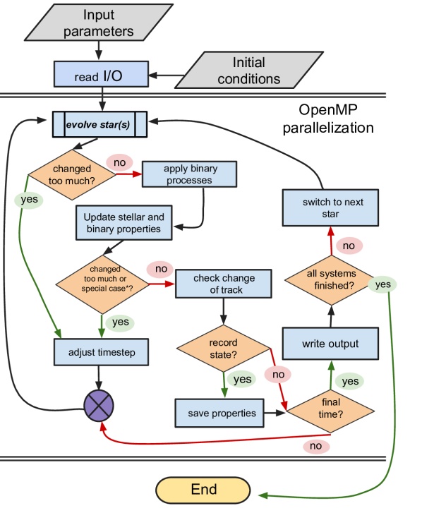
Figure 3: Schematic representation of the sevn evolution algorithm. The "changed too much" checks refer to the variation of the stellar and/or binary properties. In the case of single-stellar evolution or in the case of an ionized binary, sevn skips the sections “apply binary processes” and “update stellar and binary properties”. The “special case” check refers to all the cases in which sevn repeats the evolution to follow a particular binary evolution process, i.e, CE, merger, and circularistaion at the onset of the RLO (see Section 2.4.2 for further details).

2.4.2 Temporal evolution

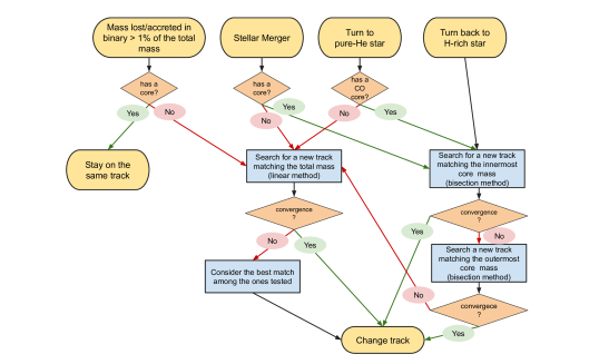
Figure 4: Schematic representation of the algorithm sevn uses during a change of stellar track (Section 2.4.3). The elements in the upper row indicate all the cases for which the code searches for a new stellar track: a significant mass loss/mass accretion due to binary interactions, a stellar merger, an H-rich star that loses its envelope turning into a pure-He star, and a pure-He star that accretes a new H envelope turning back into a H-rich star. In stars with both an He and CO cores, the latter is the innermost core. In stars with only an He core the innermost and outermost cores coincide.

Figure 3 summarises the sevn temporal evolution scheme. During each time-step, sevn evolves the two stars independently, then it evaluates and accumulates the property variations, $\Delta P$, caused by each binary-evolution process. The binary prescriptions use as input the orbital and stellar properties at the beginning of the evolution step, $P(t_{0})$.

After the integration of the binary-evolution processes, sevn updates each stellar and binary property (Fig. 3). In particular, each binary property (e.g., semi-major axis, eccentricity) is updated as $P(t)=P(t_{0})+\Delta P$.

Each stellar evolution property (e.g., mass of each star) is calculated as $P(t)=P_{\rm s}(t)+\Delta P$, where $P_{\rm s}(t)$ is the value of the property at the end of the time-step as predicted by stellar evolution only. For example, if the property $P(t)$ is the mass of an accretor star during RLO, $P_{\rm s}(t)$ is the mass predicted at the end of the time-step by stellar evolution (accounting for mass loss by winds), while $\Delta P$ is the mass accreted by RLO and by wind-mass transfer during the time-step. If necessary, the single and binary evolution step is repeated until the adaptive time-step conditions are satisfied (Section 2.4.1).

sevn evolves the compact remnants passively maintaining their properties constant. sevn treats naked-CO stars similar to compact remnants: they evolve passively until they terminate their life and turn into compact remnants.

sevn assumes that the transition from a star to a compact remnant happens at the beginning of the time-step. In this case, sevn assigns a mass and a natal kick to the new-born compact object, based on the adopted supernova model. Then, it estimates the next time-step for the updated system.

Similarly, sevn does not use the general adaptive time-step criterion when one the following processes takes place: RLO circularisation, merger, or CE. In such cases, sevn uses an arbitrarily small time-step ($\mathrm{d}t_{\mathrm{tiny}}=10^{-15}\ \mathrm{Myr}$) and calculates only the aforementioned process during such time-step. Then, it estimates the new time-step.

At the very end of each evolutionary step, sevn checks if a SNIa must take place. A SNIa is triggered if any of the following conditions is satisfied: i) a HeWD with mass larger than $0.7\ \mbox{M${}_{\odot}$}$ has accreted He-rich mass from a WR star, or ii) a COWD has accreted at least 0.15 M_⊙ from a WR star.

Furthermore, sevn checks if any ONeWD (NS) has reached a mass larger than 1.44 M_⊙ (3 M_⊙) during the time-step. If this happens, the ONeWD (NS) becomes a NS (BH). Finally, sevn checks if the stars in the binary need to jump to a new interpolating track (Section 2.4.3).

2.4.3 Change of interpolating tracks

During binary evolution, a star can change its mass significantly due to mass loss/accretion, or after a stellar merger. In these cases, sevn needs to find a new track, which better matches the current stellar properties. For stars without a core (MS H-stars or core He burning pure-He stars), sevn moves onto a new evolutionary track every time the net cumulative mass variations due to binary processes (RLO, wind mass accretion) is larger than 1% of the current star mass. When a decoupled (He or CO) core is present, its properties drive the evolution of the star (see, e.g., Hurley et al., 2000, Section 7.1). For this reason, we do not allow stars with a He or CO core (H-star with phase $>2$ and pure-He stars with phase $>4$) to change track unless the core mass has changed. After a stellar merger, sevn always moves the merger product to a new stellar track. When an H-rich star fulfils the WR star condition (He-core mass larger than 97.9% of the total mass), the star jumps to a new pure-He track.

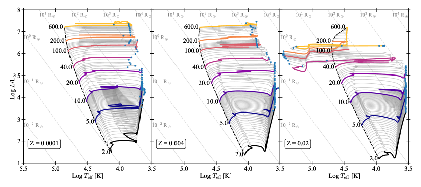
Figure 5: Hertzsprung-Russell (HR) diagram of parsec stellar tracks for three selected metallicities and $\lambda_{\mathrm{ov}}=0.5$. Different colours indicate selected tracks with initial masses $M_{\mathrm{ZAMS{}{=}}}$ 2, 5, 10, 20, 40, 100, 200 and 600 M_⊙. Solid grey lines show all the other tracks. The blue stars indicate the position of the star at the pre-supernova stage. The dashed black line shows the ZAMS. Diagonal dashed grey lines indicate points in the diagram at a constant radius.

When a star moves to a new track, sevn searches the track that best matches the mass (or the mass of the core) of the current star at the same evolutionary stage (sevn phase and percentage of life) and metallicity. We define the ZAMS mass of such a track as $M_{\mathrm{ZAMS,new}}$. In general, sevn searches the new track in the H (pure-He) tables for H-rich (pure-He) stars. The only exceptions occur when a H-rich star is turned into a pure-He star (in this case, sevn jumps to pure-He tables), and when a pure-He star is transformed back to a H-rich star after a merger (sevn jumps from a pure-He table to a H-rich table).

sevn adopts two different strategies to find the best $M_{\mathrm{ZAMS,new}}$ for stars with or without a core. For stars without a core-envelope separation, sevn finds the best $M_{\mathrm{ZAMS,new}}$ following the method implemented in Spera et al. (2019, see their Appendix A2). Hereafter, we define $M$ as the current mass of the star, $M_{\mathrm{p}}$ as the mass of the star with ZAMS mass $M_{\mathrm{ZAMS}}$, estimated at the same phase and percentage of life of the star that is changing track. $M_{\mathrm{ZAMS,old}}$ is the ZAMS mass of the current interpolating track. Assuming a local linear relation between $M_{\mathrm{ZAMS}}$ and $M_{\mathrm{p}}$, we can estimate $M_{\mathrm{ZAMS,new}}$ using equation

$$M=\frac{M_{\mathrm{p,2}}-M_{\mathrm{p,1}}}{M_{\mathrm{ZAMS,2}}-M_{\mathrm{ZAMS,1}}}(M_{\mathrm{ZAMS,new}}-M_{\mathrm{ZAMS,1}})+M_{\mathrm{p,1}}.$$ (43)

As a first guess, we set $M_{\mathrm{ZAMS,1}}=M_{\mathrm{ZAMS,old}}$ and $M_{\mathrm{ZAMS,2}}=M_{\mathrm{ZAMS,old}}+1.2\delta M$, where $\delta M$ is the cumulative amount of mass loss/accreted due to the binary processes. $M_{\mathrm{ZAMS,new}}$ is accepted as the ZAMS mass of the new interpolating track if

$$\frac{|M_{\mathrm{p,new}}-M|}{M}<0.005,$$ (44)

otherwise Eq. 43 is iterated replacing $M_{\mathrm{ZAMS,1}}$ or $M_{\mathrm{ZAMS,2}}$ with the last estimated $M_{\mathrm{ZAMS,new}}$. The iteration stops when the condition in Eq. 44 is fulfilled, or after 10 steps, or if $M_{\mathrm{ZAMS,new}}$ is outside the range of the ZAMS mass covered by the stellar tables. If the convergence is not reached, the best $M_{\mathrm{ZAMS,new}}$ will be the one that gives the minimum value of $|M_{\mathrm{p,new}}-M|/M$ (it could also be the original $M_{\mathrm{ZAMS,old}}$). sevn applies this method also when H-rich stars without a CO-core turn into pure-He stars (phase $\leq 4$). If the phase is $<4$, sevn sets the evolutionary stage of the new track at the beginning of the core-He burning (phase 4).

For stars with a core, sevn looks for the best $M_{\mathrm{ZAMS,new}}$ matching the mass of the innermost core $M_{\mathrm{c}}$ (He-core for stellar phases 2, 3, 4, and CO-core for phases 5, 6, see Table 2). For this purpose, we make use of the bisection method in the ZAMS mass range [$\max(M_{\mathrm{c}},M_{\mathrm{ZAMS,min}})$, $M_{\mathrm{ZAMS,max}}$], where $M_{\mathrm{ZAMS,min}}$ and $M_{\mathrm{ZAMS,max}}$ represent the boundaries of the ZAMS mass range covered by the stellar tables (see Sections 2.1.1 and 3.1). sevn iterates the bisection method until Eq. 44 is valid considering the core masses. If the convergence is not reached within 10 steps, sevn halts the iteration and the best $M_{\mathrm{ZAMS,new}}$ is the one that gives the best match to the core mass. Sometimes (e.g. after a merger) the CO core is so massive that no matches can be found. In those cases, sevn applies the same method trying to match the mass of the He core. If the He-core mass is not matched, sevn applies the linear iterative method to match the total mass of the star. sevn uses this method also when a pure-He star turns back to an H-rich star after accreting an hydrogen envelope or when a H-rich star with a CO core turns into a pure-He star.

Finally, the star jumps to the new interpolating track with ZAMS mass $M_{\mathrm{ZAMS,new}}$. sevn updates the four interpolating tracks and synchronises all the stellar properties with the values of the new interpolating track. The only exceptions are the mass properties (mass, He-core mass, CO-core mass). If the track-finding methods do not converge (Eq. 44 is not valid), the change of track might introduce discontinuities in these properties. To avoid this problem, Spera et al. (2019) added a formalism that guarantees a continuous temporal evolution. In practice, sevn evolves the stellar mass and mass of the cores using

$$M_{\mathrm{t_{1}}}=M_{\mathrm{t_{0}}}\,{}(1+\delta m),\ \mathrm{where}\ \delta m=\frac{m_{\mathrm{t_{1}}}-m_{\mathrm{t_{0}}}}{m_{\mathrm{t_{0}}}}.$$ (45)

In Eq. 45, $M_{\mathrm{t_{1}}}$ and $M_{\mathrm{t_{0}}}$ are the masses of the star (or of the core) estimated at time $t_{1}$ and $t_{0}$, while $m_{\mathrm{t_{1}}}$ and $m_{\mathrm{t_{0}}}$ are the masses obtained from the interpolating tracks at time $t_{1}$ and $t_{0}$ (see Section 2.1.4). Figure 4 summarises the algorithm sevn uses to check and handle a change of track.

3 Simulation setup

3.1 parsec Stellar tracks

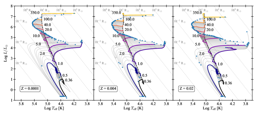
Figure 6: Same as Fig. 5 but for pure-He parsec stellar tracks.

In this work we make use of stellar evolution tracks computed with the stellar evolutionary code parsec (Bressan et al., 2012; Costa et al., 2019; Costa et al., 2021; Nguyen et al., 2022). In the following, we briefly describe the input physics assumed and the stellar tracks computed.

For the wind of massive hot stars, we use the mass-loss prescriptions by Vink et al. (2000) and Vink et al. (2001), which take into account the dependence of the mass-loss on stellar metallicity. We also include the recipes by Gräfener & Hamann (2008) and Vink et al. (2011), which include the dependence of mass-loss on the Eddington ratio. For WR stars, we use prescriptions by Sander et al. (2019), which reproduce the observed Galactic WR type-C (WC) and WR type-O (WO) stars. We modified the Sander et al. (2019) recipe, including a metallicity dependence. We refer to Costa et al. (2021) for further details. For micro-physics, we use a combination of opacity tables from the Opacity Project At Livermore (OPAL) team (Iglesias & Rogers, 1996), and the æsopus tool (Marigo & Aringer, 2009), for the regimes of high temperature ($4.2\leq{}\log{(T/{\rm K})}\leq{}8.7$) and low temperature ($3.2\leq{}\log{(T/{\rm K})}\leq{}4.1$), respectively. We include conductive opacities by Itoh et al. (2008). For the equation of state, we use the freeeos code version 2.2.1 by Alan W. Irwin, for temperature $\log{(T/{\rm K})}<8.5$. While for higher temperatures ($\log{(T/{\rm K})}>8.5$), we use the code by Timmes & Arnett (1999), in which the creation of electron-positron pairs is taken into account.

For internal mixing, we adopt the mixing-length theory (MLT, Böhm-Vitense, 1958), with a solar-calibrated MLT parameter $\alpha_{\mathrm{MLT}}=1.74$ (Bressan et al., 2012). We use the Schwarzschild criterion (Schwarzschild, 1958) to define the convective regions, with the core overshooting computed with the ballistic approximation by Bressan et al. (1981). We computed two different sets of tracks with an overshooting parameter $\lambda_{\mathrm{ov}}=0.4$ and 0.5. $\lambda_{\mathrm{ov}}$ is the mean free path of the convective element across the border of the unstable region in units of pressure scale height. For the convective envelope, we adopted an undershooting distance $\Lambda_{\mathrm{env}}=0.7$ in pressure scale heights. More details on the assumed physics and numerical methodologies can be found in Bressan et al. (2012) and Costa et al. (2021).

Using the solar-scaled elements mixture by Caffau et al. (2011), we calculated 13 sets of tracks with a metallicity ranging from $Z=10^{-4}$ to $4\times 10^{-2}$. Each set contains approximately 70 tracks with a mass ranging from 2 to 600 M_⊙. For stars in the mass range $2\,{}\mbox{M${}_{\odot}$}\ <\mbox{$M_{\mathrm{ZAMS{}{}}}$}<8\,{}\mbox{M${}_{\odot}$}$, we follow the evolution until the early asymptotic giant branch (E-AGB) phase. Stars with an initial mass $\mbox{$M_{\mathrm{ZAMS{}{}}}$}>8\,{}\mbox{M${}_{\odot}$}{}$ are computed until the advanced core O-burning phase or the beginning of the electron-positron pair instability process. Figure 5 shows sets of tracks with different metallicities and with the overshooting parameter $\lambda_{\mathrm{ov}}=0.5$.

We also computed new pure-He stellar tracks with parsec. For pure-He stellar winds, we adopted the prescriptions from Nugis & Lamers (2000). More details can be found in Chen et al. (2015). The new sets are computed with the same input physics used for standard stars. The initial composition is set as follows. The hydrogen mass fraction is set to zero ($X=0$), the helium mass fraction is given by $Y=1-Z$, and the metallicity ($Z$) ranges from 10^-4 to $5\times 10^{-2}$. Each set contains 100 tracks with masses ranging from $\mbox{$M_{\mathrm{ZAMS{}{}}}$}=0.36$ M_⊙ to 350 M_⊙. Figure 6 shows three selected sets of pure-He tracks with different metallicity. These sets of tracks are part of a database that will be described in Costa et al. (in prep.), and will be publicly available in the new parsec Web database repository.

We used the code TrackCruncher (Section 2.1.1) to produce look-up tables for sevn from the parsec stellar tracks (see Appendix B for additional details). The parsec tables contain the stellar properties: mass, radius, luminosity, He and CO core mass and radius. The He/CO core masses and radii are estimated considering the point at which the H/He mass fraction drops below 0.1%. In addition, we produced tables for the properties of the convective envelope (mass, extension, eddy turnover timescale, see Section 2.1.1). For the stellar inertia we use Eq. 8, while for the binding energy we use Eq. 32 and test four different assumptions for the parameter $\lambda_{\mathrm{CE}}$ (Section 3.2).

3.1.1 parsec and mobse stellar track comparison

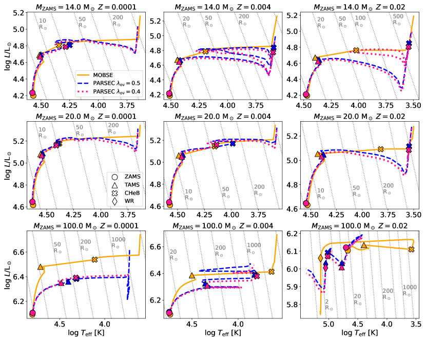
Figure 7: Comparison of stellar tracks in the HR diagram computed by mobse (orange solid lines), and sevn using parsec stellar tables with overshooting parameter $\lambda_{\mathrm{ov}}=0.5$ (blue dashed lines) and $\lambda_{\mathrm{ov}}=0.4$ (pink dotted lines). The panels’ titles specify the zero-age MS (ZAMS) mass and metallicity of the computed tracks. The markers indicate peculiar phases during the stellar evolution: starting position in the ZAMS (ZAMS, circles); terminal-age MS, i.e. the first time the He-core decouples from the envelope (TAMS, triangles); helium burning ignition in the core (CHeB, crosses); begin of WR star evolution, i.e. bse phase 7 (WR, diamonds, see Section 2.1.3). The grey dashed lines indicate points at constant radius: 1, 2, 5, 10, 20, 50, 100, 200, 500, 1000, and 2000 R_⊙. sevn evolves the WR stars using the pure-He stellar tracks (Section 2.4.3), therefore the PARSEC lines after the diamonds are computed interpolating the pure-He tables (Fig. 6).

The stellar evolution implemented in mobse and other bse-like population synthesis codes is based on the stellar evolution tracks computed by Pols et al. (1998). Figure 7 shows the comparison of the stellar evolution tracks computed with mobse, and sevn using the parsec tracks for three selected ZAMS masses (14 M_⊙, NS progenitors; 20 M_⊙, transition between NS/BH progenitors; 100 M_⊙, high-mass BH progenitors) at three different metallicities: $Z=0.0001$, 0.004, and 0.02.

In most cases, the mobse and sevn+parsec stellar tracks show significant differences, especially for the metal-rich stars. In the high-mass range of the NS progenitors ($14\lesssim M_{\mathrm{ZAMS}}/\mbox{M${}_{\odot}$}\lesssim 20$), the evolution differs substantially after the MS (top panels and middle-right panel in Fig. 7). In particular, in both parsec models, the stars ignite helium in the red part of the Hertzsprung-Russell (HR) diagram ($T_{\mathrm{eff}}\approx 3000$ K), while in mobse core He burning begins in a bluer region ($T_{\mathrm{eff}}\gtrsim 5600$ K) when the stars are still relatively small ($R\lesssim 200\ \mbox{R${}_{\odot}$}$).

Figure 7 shows that the star with $M_{\mathrm{ZAMS}}=14\ \mbox{M${}_{\odot}$}$ ignites helium in an even bluer position in the HR at $T_{\mathrm{eff}}\approx 10^{4}$ K, when it has a radius of $\approx 70\ \mbox{R${}_{\odot}$}$. Therefore, in mobse, the NS progenitors tend to interact with their binary companion after or during the core He burning phase. In contrast, when sevn makes use of the parsec tracks, most of the NS progenitors interact before helium ignition, i.e., during the Hertzsprung gap or giant branch phase (bse types 2 and 3, see Table 2). Since most binary-evolution processes depend on the stellar type (e.g., RLO, Section 2.3.2), these differences have a dramatic impact on the production of BNSs (Sections 4.2.3 and 4.3.2).

The parsec stellar tracks with different $\lambda_{\mathrm{ov}}$ values show a similar evolution in the HR diagram. The largest differences are in the mass range of the NS progenitors at high metallicity. For these stars, the tracks with $\lambda_{\mathrm{ov}}=0.4$ produce a much more extend blue loop (see, e.g., the top-right panel in Fig. 7). The blue loop is a typical feature of stars in this mass range: at the ignition of core helium burning the star contracts moving to the blue part of the HR diagram, then it expands again at the end of the core He burning toward the asymptotic giant branch. The $\lambda_{\mathrm{ov}}=0.4$ and $\lambda_{\mathrm{ov}}=0.5$ models are similar in many respects, hence we use the term parsec referring to both models, unless specifically noted.

Overall, the mobse stellar tracks reach larger radii during the evolution (up to ten times). In particular, high-mass BH progenitors ($M_{\mathrm{ZAMS}}\gtrsim 50\ \mbox{M${}_{\odot}$}$) in mobse expand up to 2500–10000 R_⊙, while in parsec the maximum radius ranges from $\approx 50\ \mbox{R${}_{\odot}$}$ (for $Z\gtrsim 0.02$) to $\approx 2500\ \mbox{R${}_{\odot}$}$ (for $Z\lesssim 0.001$) (see, e.g., the lower panels in Fig. 7). However, in parsec very high-mass ($M_{\mathrm{ZAMS}}\gtrsim 100\ \mbox{M${}_{\odot}$}$) metal-poor ($Z\lesssim 0.002$) stars reach large radii (up to $\approx 2500\ \mbox{R${}_{\odot}$}{}$) during the MS, while in mobse such stars do not expand more than $\approx 50\ \mbox{R${}_{\odot}$}{}$ before the end of the MS (see lower-left panel in Fig. 7). Therefore, in the sevn+parsec simulations massive metal-poor stars tend to interact with their binary companion during the MS, while in mobse this happens at later evolutionary stages.

In mobse, high-mass metal-rich stars that become WR stars during the stellar evolution always expand up to 1000–4000 R_⊙ before helium ignition, then they contract and move toward the blue part of the HR diagram. In parsec, only stars with $Z<0.007$ or $M_{\mathrm{ZAMS}}\lesssim 70\ \mbox{M${}_{\odot}$}$ expand significantly (up to $\approx 1000$ R_⊙) before the WR star phase, the other stars contract and move to the blue part of the HR diagram already during the evolution in the MS (see bottom panels in Fig. 7). As a consequence, high-mass metal-rich stars in sevn+parsec simulations interact less frequently with their binary companion with respect to mobse.

In the mass range of the NS progenitors ($\approx$ 8–20 M_⊙) at low ($Z<0.001$) and intermediate-high metallicity ($Z>0.003$), the mobse-parsec difference in the maximum stellar radius decreases to $\approx$ 0–200 R_⊙ (see, e.g., the middle-top panel in Fig. 7). There is a small region in the ZAMS mass-metallicity plane ($0.004\lesssim Z\lesssim 0.008$ and $20\lesssim M_{\mathrm{ZAMS}}/\mbox{M${}_{\odot}$}\lesssim 30$), where the parsec stellar tracks reach radii larger than 200–400 R_⊙ with respect to mobse.

The stellar mass at the end of the star lifetime ($M_{\mathrm{f}}$) is larger in parsec (up to $\approx{40}$%) for massive stars ($M_{\mathrm{ZAMS}}\gtrsim 100\ \mbox{M${}_{\odot}$}$) and/or stars with high metallicity ($Z>0.008$). At intermediate metallicities ($0.001<Z<0.008$), mobse produces larger final masses (up to $\approx 25$%) in the mass range 70–100 M_⊙. The $M_{\mathrm{f}}$ differences between the two parsec models are within $\approx{10}$% without a clear trend with $M_{\mathrm{ZAMS}}$ and $Z$.

The final masses of the He and CO cores are similar in the mass range 8–30 M_⊙. More massive cores ($\lesssim 30$%) are produced by mobse for $M_{\mathrm{ZAMS}}<8\ \mbox{M${}_{\odot}$}$ and by parsec for $M_{\mathrm{ZAMS}}>30\ \mbox{M${}_{\odot}$}$.

At low metallicity ($Z\lesssim 0.001$), in the ZAMS mass range 100–150 M_⊙, the parsec stellar tracks with $\lambda_{\mathrm{ov}}=0.5$ end their life with lighter cores ($\approx 25\%$) with respect to mobse and parsec with $\lambda_{\mathrm{ov}}=0.4$. This feature, produced by the dredge-up and the envelope undershooting (see, e.g., Costa et al., 2021), has a large impact on the mass of the compact remnant when combined with the PISN formalisms (Section 4.1.1). In the rest of the metallicity and ZAMS range, the parsec models with $\lambda_{\mathrm{ov}}=0.5$ produce slightly ($3\%-5\%$ on average) more massive cores at the end of the evolution with respect to models with $\lambda_{\mathrm{ov}}=0.4$.

The stellar lifetime in parsec is shorter with respect to mobse up to 25% for $M_{\mathrm{ZAMS}}\lesssim 80\ \mbox{M${}_{\odot}$}$, and up to 40% for $M_{\mathrm{ZAMS}}\gtrsim 80\ \mbox{M${}_{\odot}$}$. For $Z<0.01$, the parsec models with $\lambda_{\mathrm{ov}}=0.5$ have a slightly longer lifetime ($\approx 5\%$) with respect to models with $\lambda_{\mathrm{ov}}=0.4$. This difference increases up to $\approx 15\%$ for massive stars ($M_{\mathrm{ZAMS}}\gtrsim 200\ \mbox{M${}_{\odot}$}$).

Using sevn+parsec the ZAMS mass for the WD/NS transition (Section 2.2) increases with metallicity from $\approx 8\ \mbox{M${}_{\odot}$}{}$ at $Z=0.0001$ to $\approx 9\ \mbox{M${}_{\odot}$}{}$ at $Z=0.02$. The NS/BH mass transition is at $\approx 23\ \mbox{M${}_{\odot}$}{}$ for the rapid supernova model and at $\approx 18\mathrm{-}19\ \mbox{M${}_{\odot}$}{}$ for the delayed model (see Section 2.2.1). In mobse, the WD/NS and the NS/BH mass transitions shift to lower masses: from $\approx 6\ \mbox{M${}_{\odot}$}{}$ ($Z=0.0001$) to $\approx 7.5\ \mbox{M${}_{\odot}$}{}$ ($Z=0.02$) for the WD/NS boundary, and from $\approx 20\ \mbox{M${}_{\odot}$}{}$ ( $\approx 17\ \mbox{M${}_{\odot}$}{}$) to $\approx 22\ \mbox{M${}_{\odot}$}{}$ ( $\approx\ 20\mbox{M${}_{\odot}$}{}$) for the NS/BH transition assuming the rapid (delayed) supernova model (see, e.g., Fig. 1 in Giacobbo & Mapelli, 2018). Given a stellar population following a Kroupa initial mass function (Section 3.3) and considering only single stellar evolution, mobse produces a larger number of NSs ($\approx 10\mathrm{-}30\%$) and BHs ($\approx 5\mathrm{-}20\%$) with respect to sevn+parsec.

In Appendix C, we compare the parsec stellar tracks with the ones from other recent stellar evolution/population synthesis codes (mist, Choi et al. 2016; combine, Kruckow et al. 2018; posydon, Fragos et al. 2023).

3.2 Setup models

We explore the uncertainties produced by binary evolution prescriptions using 15 different setup models for the parameters of the sevn simulations.

Unless otherwise specified, we use the parsec stellar tables with $\lambda_{\mathrm{ov}}=0.5$ for the evolution of H-rich star, and the parsec pure-He tables for the evolution of pure-He stars. In addition to the fundamental look-up tables (stellar mass, He and CO core mass, radius, luminosity), we use the stellar tables to evaluate the radial extension of the He and CO cores, and to follow the evolution of the convective envelope properties (mass fraction, depth of the convective layers and eddy turnover timescale, see Section 2.1.1).

For the fiducial model (F), we set all sevn parameters to their default values (see Sections 2.1 and 2.3). We use the rapid supernova model by Fryer et al. (2012), but we draw the NS masses from a Gaussian distribution centred at $M=1.33\ \mbox{M${}_{\odot}$}$ (Section 2.2.1). We take into account the pair instability and pulsation pair instability using the model M20 by Mapelli et al. (2020) (Section 2.2.2). We use the model KGM20 by Giacobbo & Mapelli (2020) to draw the natal kicks (Section 2.2.4). We use the option QCRS (Table 3) for the stability of the mass transfer during the RLO, hence the mass transfer is always stable for MS and HG donor stars (bse phases 1 and 2, see Table 2), while we follow the Hurley et al. (2002) prescriptions in all the other cases. We set the default RLO mass accretion efficiency to $f_{\rm MT}=0.5$ (Eq. 25) as the mean of the interval, and assume that the mass not accreted during the RLO is lost from the vicinity of the accretor as an isotropic wind (isotropic re-emission option, see Appendix A.4.2). At the onset of RLO, sevn circularises the orbit at periastron (Section 2.3.5). During CE, we estimate the envelope binding energy (Eq. 32) using the same $\lambda_{\mathrm{CE}}$ formalism as in mobse and bse (see Appendix A.1.4).

Model	Parameter variations
F	Fiducial model
QCBSE	Use QCBSE option for the RLO mass transfer stability (Table 3)
QCBB	Use QCBB option for the RLO mass transfer stability (Table 3)
QHE	Enable quasi-homogeneous evolution during RLO (Section 2.3.2)
RBSE	Use Eq. 26 for mass accretion efficiency during the RLO (same as in Hurley et al. 2002)
K$\sigma 265$	Draw supernova kicks from a Maxwellian with $\sigma=265\ \mathrm{km}{s}^{-1}$
K$\sigma 150$	Draw supernova kicks from a Maxwellian with $\sigma=150\ \mathrm{km}{s}^{-1}$
F19	Use Farmer et al. (2019) PISN prescriptions (Section 2.2.2)
SND	Use the delayed supernova model with a Gaussian distribution
	for NS masses (Section 2.2.1)
NT	Disable tides (Section 2.3.4)
NTC	Disable tides and circularise when the RLO condition is valid at the pericentre (Section 2.3.5)
LK	Use $\lambda_{\mathrm{CE}}$ by Klencki et al. (2021) for CE (Eq. 32)
LX	Use $\lambda_{\mathrm{CE}}$ by Xu & Li (2010b) for CE (Eq. 32)
LC	Use $\lambda_{\mathrm{CE}}=0.1$ for CE (Eq. 32)
OPT	QCBSE + Optimistic CE assumption for HG stars (Section 2.3.3)

Table 5: List of the 15 setup models used in this work to set the sevn single and binary stellar evolution parameters. Column 2 (Parameter variations) describes what we change in each model with respect to the fiducial model. The fiducial model (F) is described in the main text (Section 3.2).

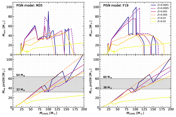
Figure 8: Compact remnant mass and pre-supernova core masses from single stellar evolution as a function of the initial mass $M_{\mathrm{ZAMS}}$ for the look-up tables obtained from parsec stellar tracks with $\lambda_{\mathrm{ov}}=0.5$ (Section 3.1). The upper-left and upper-right panels show the mass of the compact remnant considering the pair-instability model M20 and F19, respectively (Section 2.2.2). In both cases, we adopt the rapid supernova model (Section 2.2.1). The lower panels show the pre-supernova mass of the He core, $M_{\mathrm{He}}$ (left-hand panel), and CO core, $M_{\mathrm{CO}}$ (right-hand panel). The dashed horizontal lines mark the fundamental mass thresholds for the PISN models. In the model M20, we expect the star to undergo pulsational pair instability (PPI) between $32\ \mbox{M${}_{\odot}$}\leq M_{\mathrm{He}}\leq 64\ \mbox{M${}_{\odot}$}$, while for $M_{\mathrm{He}}>64\ \mbox{M${}_{\odot}$}$ the star explodes as a PISN leaving no compact remnant. In F19, the PPI and PISN windows start at $M_{\mathrm{CO}}\geq 38\ \mbox{M${}_{\odot}$}$ and $M_{\mathrm{CO}}>60\ \mbox{M${}_{\odot}$}$, respectively. The different lines indicate different metallicities: $Z$=0.0001 blue solid line, $Z$=0.0005 violet dashed line, $Z=$0.001 violet solid line, $Z$=0.005 orange dashed line, $Z$=0.01 orange solid line, $Z$=0.02 yellow solid line. The $M_{\mathrm{ZAMS}}$ of the evolved stars are sampled each 0.5 M_⊙ in the interval 2.5–200 M_⊙.

Table 5 summarises all the other 14 models and their variations with respect to the fiducial model. We test alternative assumptions for the RLO stability with the models QCBSE and QCBB (see Table 3), the model QHE enables the quasi-homogeneous evolution after the RLO mass transfer, while in the model RBSE we set the efficiency of the RLO mass transfer same as in mobse using Eq. 26 (most of the time it is equivalent to a conservative mass transfer, i.e. $f_{\mathrm{MT}}\approx 1$ in Eq. 25.).

The models K$\sigma 265$ and K$\sigma 150$ test alternative natal kicks, drawn from a Maxwellian distribution with one-dimensional root-mean square $\sigma_{\rm kick}=265$ and 150 km s^-1, respectively. In model F19, we replace the M20 PISN model with the Farmer et al. (2019) prescriptions. In model SND we explore the delayed supernova model by Fryer et al. (2012), drawing the NS masses from a Gaussian distribution.

We investigate the impact of the stellar tides disabling them in the model NT. In the model NTC, we disable the tides and use a less stringent criterion to trigger binary circularisation, enabling it every time the RLO condition is valid at periastron, i.e. using the periastron distance instead of the semi-major axis in Eq. 21 (Section 2.3.5). Furthermore, we test different prescriptions to evaluate $\lambda_{\mathrm{CE}}$ during CE with the model LX (based on Xu & Li 2010b), LK (based on Klencki et al. 2021), and LC (in which $\lambda_{\mathrm{CE}}=0.1$, see Appendix A.1.4). Finally, model OPT is the closest set-up to the standard bse formalism (Hurley et al., 2002): we assume the same mass-transfer stability criteria as bse (QCBSE), and we allow HG donors to survive a CE phase (optimistic CE assumption).

3.3 Initial conditions

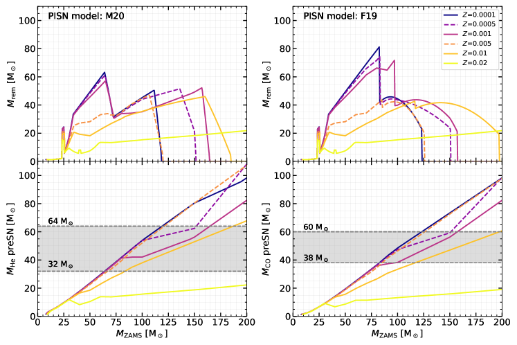
Figure 9: Same as Fig. 8, obtained from parsec stellar tracks with $\lambda_{\mathrm{ov}}=0.4$ (see Section 3.1).

We randomly draw the initial ZAMS masses of primary stars from a Kroupa initial mass function (IMF, Kroupa 2001)

$$\mathrm{pdf}(M_{\mathrm{ZAMS,1}})\propto M_{\mathrm{ZAMS,1}}^{-2.3}\ \ \ \ \ M_{\mathrm{ZAMS,1}}\in\ [5,150]\ \mathrm{M}_{\odot},$$ (46)

and the masses of secondary stars assuming the distribution of mass ratios from Sana et al. (2012), based on observations of O- and B-type binary stars in open clusters:

$$\mathrm{pdf}(q)\propto q^{-0.1}\ \ \ \ \ q=\frac{M_{\mathrm{ZAMS,2}}}{M_{\mathrm{ZAMS,1}}}\in[q_{\mathrm{min}},1.0]\ \mathrm{M}_{\odot},$$ (47)

with

$$q_{\mathrm{min}}=\max\left(\frac{2.2}{M_{\mathrm{ZAMS,1}}},0.1\right)$$ (48)

The lower mass limits for primary stars (5 M_⊙) and secondary stars (2.2 M_⊙) represent safe boundaries to study NSs and BHs. The upper mass limit (150 M_⊙) is a typical mass limit used in the study of NSs and BHs (e.g. Giacobbo & Mapelli, 2018; Spera et al., 2019). The parsec tracks used in this work reach masses up to 600 M_⊙. We investigate this high mass regime in the follow-up paper Costa et al. (2023). We set the initial rotational velocity of the stars to 0.

The initial orbital periods ($P$) and eccentricities ($e$) have been generated according to the distributions by Sana et al. (2012):

$$\mathrm{pdf}(\mathcal{P})\propto\mathcal{P}^{-0.55}\ \ \ \ \ \mathcal{P}=\log(P/\mathrm{day)}\in[0.15,5.5],$$ (49)

$$\mathrm{pdf}(e)\propto e^{-0.42}\ \ \ \ \ e\in[0,0.9].$$ (50)

We generate $10^{6}$ binary systems and use them as initial conditions in all our simulations (i.e., for different metallicities and different combinations of the main parameters).

The total mass of the simulated binaries is $2.21\times 10^{7}\ \mbox{M${}_{\odot}$}$ corresponding to an effective total mass of $1.74\times 10^{8}\ \mbox{M${}_{\odot}$}$ when taking into account the correction for incomplete IMF sampling due to the mass cuts ($f_{\rm cut}=0.255$)

For each of the 15 setup models (see Table 5), we ran 60 sets of simulations combining 15 metallicities ($Z=10^{-4}$, $2\times 10^{-4}$, $4\times 10^{-4}$, $6\times 10^{-4}$, $8\times 10^{-4}$, $10^{-3}$, $2\times 10^{-3}$, $4\times 10^{-3}$, $6\times 10^{-3}$, $8\times 10^{-3}$, $10^{-2}$, $1.4\times 10^{-2}$, $1.7\times 10^{-2}$, $2\times 10^{-2}$, $3\times 10^{-2}$) and four values for the $\alpha_{\mathrm{CE}}$ parameter ($\alpha_{\mathrm{CE}}=0.5$, 1, 3, 5). In addition to the 15 models, we generate an extra set of $5\times 10^{6}$ binaries, then we simulate them using the fiducial model (Section 3.2). We use this supplementary dataset to investigate the systematic uncertainties originated by the sampling of the initial conditions. In conclusion, we simulate a total of $1.2\times 10^{9}$ binary systems.

We use sevn to evolve all the binaries until both stars are compact remnants or, if they collide, until their merger product becomes a compact remnant. For a BCO, the orbital decay by GWs is the only active process (Section 2.3.6). Therefore, for each BCO, we estimate the merger time a posteriori using $t_{\mathrm{merge}}$ (Eq. 75). Using 10 threads on a server equipped with Intel(R) Xeon(R) Platinum 8168 (2.70 Ghz) CPUs, sevn completed the evolution of each set of $10^{6}$ binaries in approximately 1 hour.

The list of initial conditions, the script used to run SEVN, and the simulations outputs are available in Zenodo (Iorio et al., 2023).

4 Results

4.1 Compact remnant mass

4.1.1 Single star evolution

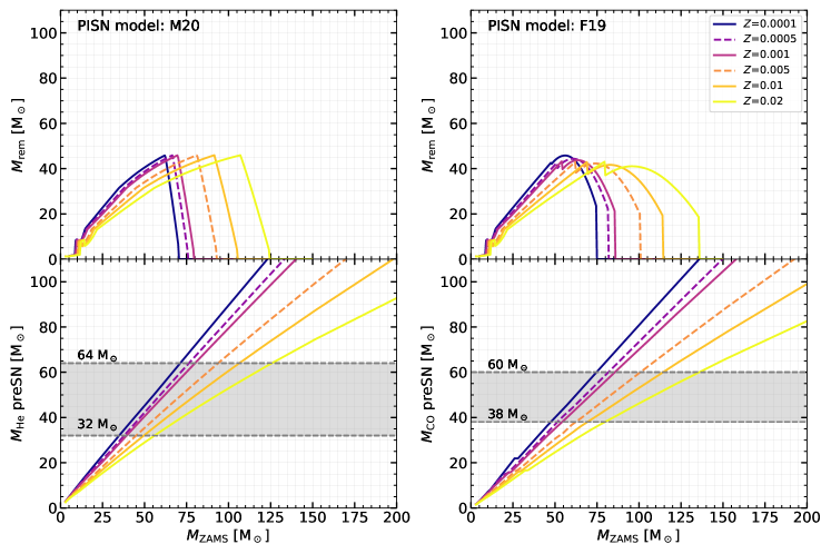
Figure 10: Same as Fig. 8, but for the parsec pure-He look-up table (see Section 3.1). $M_{\mathrm{ZAMS}}$ indicates the initial mass at the beginning of the core He burning, while the $M_{\mathrm{He}}$ is equivalent to the pre-supernova stellar mass.

Figures 8 and 9 show the mass spectrum of compact objects that we obtain from single star evolution, by assuming input tables with $\lambda{}_{\rm ov}=0.5$ and 0.4, respectively. For each set of evolutionary tables, we show the results of both PISN models, M20 and F19 (Section 2.2.2). These figures show how sensitive the maximum mass of the BH and the PISN window are to the details of stellar evolution (e.g., Farmer et al., 2019, 2020; Mapelli et al., 2020; Renzo et al., 2020a; Costa et al., 2021; Vink et al., 2021).

In the tables with $\lambda_{\rm ov}=0.5$, several stellar models undergo a dredge-up (e.g., $M_{\rm ZAMS}\approx{100}$ and 150 M_⊙ at $Z=10^{-4}$, see Section 3.1.1). Because of the dredge-up, the final mass of the He and CO cores of these stars are smaller than those of lower-mass stars, resulting in a non-monotonic trend of both $M_{\rm He,f}$ and $M_{\rm CO,f}$ as a function of $M_{\rm ZAMS}$ (lower panels of Fig. 8). If $M_{\rm ZAMS}\approx{100}$ M_⊙ and $Z=10^{-4}$, the decrease of $M_{\rm He}$ and $M_{\rm CO}$ caused by the dredge-up allows the stellar models to avoid PPI, producing BHs with mass up to 90 and 100 M_⊙ in the M20 and F19 models, respectively. If $M_{\rm ZAMS}\approx{150}$ M_⊙ and $Z=10^{-4}$, the star avoids complete disruption by a PISN and collapses to BH after PPI. The details of the mass spectrum rely on the assumed PISN models (M20 and F19), because we do not perform hydrodynamical simulations and should be taken just as indicative trends. Moreover, here we assume that the mass of a BH formed via direct collapse is equal to the total mass of the progenitor star at the onset of core collapse (based on Fryer et al. 2012). This is an optimistic assumption, because the residual H-rich envelope is loosely bound and even a small shock triggered by neutrino emission can lead to the ejection of the outer layers (e.g., Fernández et al., 2018; Renzo et al., 2020b; Costa et al., 2022).

In contrast, for $Z<0.02$, $M_{\rm He,f}$ and $M_{\rm CO,f}$ have a perfectly monotonic trend with $M_{\rm ZAMS}$ in the tables with $\lambda_{\rm ov}=0.4$. This results in a much smoother behaviour of $M_{\rm rem}$ versus $M_{\rm ZAMS}$. In this set of tables, the M20 and F19 models lead to a maximum BH mass of $\approx{63}$ and 81 M_⊙ (at $Z=10^{-4}$), respectively.

Overall, the F19 model leads to a larger maximum mass, because the PPI regime starts at higher stellar masses with respect to M20. This result confirms that there are major uncertainties on the lower edge of PISN mass gap from stellar evolution theory (e.g., Farmer et al., 2019, 2020; Renzo et al., 2020a; Mapelli et al., 2020; Costa et al., 2021; Vink et al., 2021).

Farmer et al. (2019) do not find such large maximum BH masses, because they simulate only pure-He stars. Figure 10 shows the compact remnant mass, as a function of $M_{\rm ZAMS}$, that we obtain from our pure-He models. Here, the maximum BH mass is $M_{\rm rem}\approx{45}$ M_⊙ for both M20 and F19, with very little dependence on $Z$, as already discussed by Farmer et al. (2019).

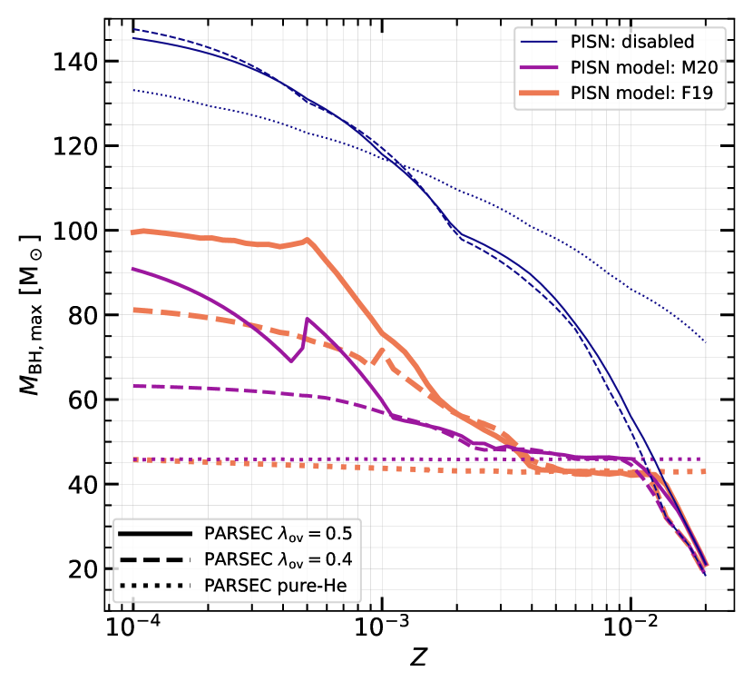
Figure 11: Maximum BH mass from single stellar evolution as function of metallicity. We estimate the BH mass using the rapid supernova model (Section 2.2.1) and different models for pair instability. No pair-instability correction: very thin blue lines; M20 (based on Mapelli et al. 2020): thin violet lines; F19 (based on Farmer et al. (2019)): thick orange lines. See Section 2.2.2 for details on pair-instability models. The plot shows the results for three different parsec look-up tables: two sets of H-rich stars (from parsec tracks with $\lambda_{\mathrm{ov}}=0.5$, solid lines, and $\lambda_{\mathrm{ov}}=0.4$, dashed lines), and one for pure-He stars (dotted lines). See Section 3.1 for additional details on the stellar tracks. We sample the $M_{\mathrm{ZAMS}}$ each 0.5 M_⊙ in the interval 2.5–200 M_⊙, while the 50 used metallicities are uniformly sampled in the logarithmic space between $Z=0.0001$ and $Z=0.02$. For pure-He stars, $M_{\mathrm{ZAMS}}$ indicates the initial mass at the beginning of the core He burning.

Figure 11 shows the maximum BH mass ($M_{\rm BH,\,{}max}$) that we obtain in our models as a function of metallicity. Here, we do not consider BHs above the upper edge of the PISN mass gap, that we discuss in Costa et al. (2023). In the H-rich models, $M_{\rm BH,\,{}max}$ increases for decreasing metallicity, because the residual H-rich envelope mass is larger at lower $Z$. In contrast, $M_{\rm BH,\,{}max}$ is almost independent of $Z$ for pure-He stars.

In the rapid model (Fryer et al., 2012), BH progenitors with $M_{\rm CO,f}\in{[6,\,{}7]}$ M_⊙ (corresponding to a ZAMS mass $M_{\mathrm{ZAMS}}\approx 25~{}\mbox{M${}_{\odot}$}$ ) end their life with a direct collapse producing large BH masses ($M_{\mathrm{rem}}\approx 20-25~{}\mbox{M${}_{\odot}$}$), well visible in Figs. 8 and 9. At high metallicity ($Z=0.02$), $M_{\rm CO,f}<7$ M_⊙ between $M_{\mathrm{ZAMS}}\approx 35~{}\mbox{M${}_{\odot}$}$ and $M_{\mathrm{ZAMS}}\approx 45~{}\mbox{M${}_{\odot}$}$, and $M_{\rm CO,f}<6$ M_⊙ around $M_{\mathrm{ZAMS}}\approx 40~{}\mbox{M${}_{\odot}$}$, resulting in the fast oscillations of $M_{\mathrm{rem}}$ visible in Figs. 8 and 9.

4.1.2 Binary evolution

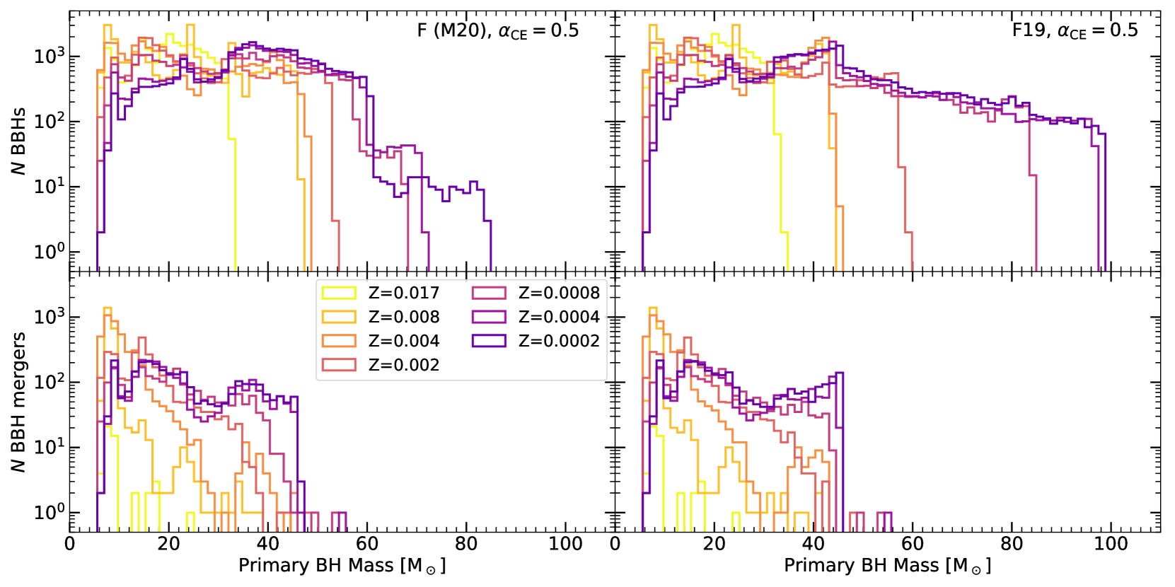
Figure 12: Upper (Lower) panel: BBHs (BBH mergers) in our simulations F (left, pair instability model M20) and F19 (right) with $\alpha_{\rm CE}=0.5$. The colour map refers to the metallicity of the progenitor ($Z=0.017$, 0.008, 0.004, 0.002, 0.0008, 0.0004, and 0.0002). The alternative versions of this plot showing the results for all the $\alpha_{\mathrm{CE}}$ values, and for all the setup models can be found in the gitlab repository of the paper ().

Figure 12 shows the distribution of primary BH masses at the end of our binary-evolution simulations. The upper panel shows all the bound BBHs, while the lower panel shows the sub-sample of BBHs that reach coalescence within the lifetime of the Universe ($\approx{14}$ Gyr, Aghanim et al. 2020). We also compare the models M20 (hereafter, fiducial model F) and F19.

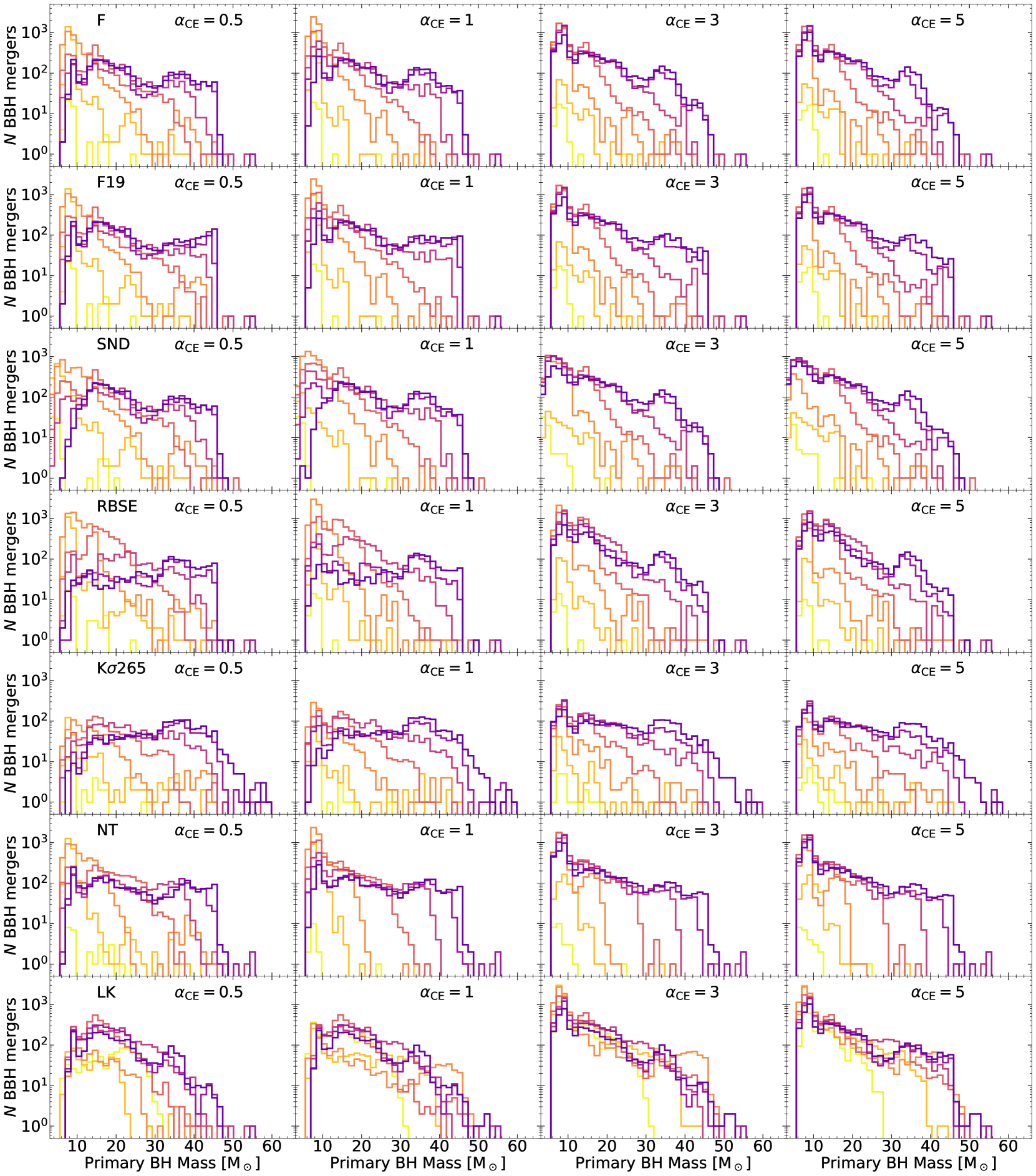
Figure 13: BBH mergers in our simulations. From left to right: $\alpha_{\rm CE}=0.5,$ 1, 3 and 5. The colour map refers to the metallicity $Z$ of the progenitor and is the same as in Fig. 12 ($Z=0.017$, 0.008, 0.004, 0.002, 0.0008, 0.0004, and 0.0002). From top to bottom we show the models F, F19, SND, RBSE, K$\sigma{}$265, NT, and LK.

The maximum BH mass depends on metallicity: higher (lower) mass BHs form from metal-poor (metal-rich) stars because of stellar winds. Binary evolution processes do not change this result, as already reported by many previous studies (Dominik et al., 2012; Mapelli et al., 2013; Giacobbo & Mapelli, 2018; van Son et al., 2023).

The maximum mass of the primary BH in loose BBH systems can be significantly higher than that of the primary BH in BBH mergers. This mainly springs from the assumption that any residual H-rich envelope collapses to a BH directly if the core-collapse supernova fails. In fact, when a binary star is tight enough to evolve into a BBH merger, it undergoes several mass transfer and/or CE phases, which lead to the complete ejection of the stellar envelope. Hence, the two resulting BHs form out of the naked cores of the two progenitor stars, and their mass cannot be $\gg{50}$ M_⊙ (Giacobbo & Mapelli, 2018).

In contrast, metal-poor single massive stars and massive stars in loose binary systems do not dissipate mass via RLO/CE, retaining a portion of their H-rich envelope until the onset of core collapse, and can directly collapse to BHs. Hence, the maximum BH mass in loose binary systems is $\approx{80}$ M_⊙ ($\approx{100}$ M_⊙) in the M20 (F19) scenario.

This effect can contribute to dilute the PISN mass gap, because the genuine edge of the PISN (i.e., the maximum mass of a BH born from a single massive star) starts at $\approx{80-100}$ M_⊙, but the maximum mass of BHs in tight binary systems (BBH mergers from isolated binary star evolution) is only $\approx{50}$ M_⊙.

The third GW transient catalogue (hereafter, GWTC-3) shows that most primary BH masses in BBH mergers are $\leq{}40$ M_⊙ (Abbott et al., 2023). This threshold might indicate that most BBH mergers in GWTC-3 come from isolated binary evolution and suffered from mass transfer and/or CE. However, in dense star clusters, some of the BHs formed from single stars and loose BBHs might pair up with other BHs and produce merging systems with primary mass up to 80–100 M_⊙ (e.g., Mapelli, 2016; Di Carlo et al., 2019; Di Carlo et al., 2020a, b; Banerjee, 2021; Torniamenti et al., 2022). The long tail in the mass spectrum of primary BHs in GWTC-3, extending up to $\sim{80}$ M_⊙ (Abbott et al., 2023) might be populated by such oversized stellar-born BHs, rather than by hierarchical mergers (e.g., Miller & Hamilton, 2002; Giersz et al., 2015; Fragione & Loeb, 2019; Fragione & Silk, 2020; Fragione et al., 2020; Kremer et al., 2020b; Mapelli et al., 2021; Mapelli et al., 2022; Mehta et al., 2022; Arca Sedda et al., 2021a; Arca Sedda et al., 2020; Arca Sedda, 2020) or primordial BHs (e.g., Carr & Hawking, 1974; Carr et al., 2016; Bird et al., 2016; Ali-Haïmoud et al., 2017; Scelfo et al., 2018; De Luca et al., 2021a, b; Franciolini et al., 2022; Ng et al., 2022).

Figure 13 shows the distribution of primary BH masses in BBH mergers, according to some of the main runs performed in this work. All the considered models show a common trend: the percentage of low-mass primary BHs increases for larger values of $\alpha_{\mathrm{CE}}$, especially at low $Z$. In fact, low values of $\alpha_{\mathrm{CE}}$ tend to facilitate the premature coalescence of a binary system during CE. This suppresses the formation of low-mass BBHs, because their stellar progenitors have relatively small radii and easily merge during CE. In contrast, the efficiency of semi-major axis shrinking drops for large values of $\alpha_{\mathrm{CE}}$, favouring the survival of both low-mass and high-mass BBHs. The number of high-mass primary BHs ($>20$ M_⊙) increases as $Z$ decreases (especially for $\alpha_{\rm CE}\leq{}1$) because only the most massive BHs merge within the Hubble time at low $Z$ (Costa et al., 2023).

At metallicity $Z\leq{}0.0004$, all our models show a local peak of the primary BH mass distribution at $35-45$ M_⊙, reminiscent of the excess found in GWTC-3 (Abbott et al., 2023; Farah et al., 2023; Callister & Farr, 2023). In model F19, the peak is shifted toward larger values ($\approx{45}$ M_⊙) than for all of the other models, because of the different treatment of PISNe. Our result suggests that the peak at $35-40$ M_⊙ in the primary BH mass distribution is produced by the interplay between the PISN model and the maximum He core mass of merging BBH progenitors at a given metallicity.

Low-mass BBH mergers are rare in models K$\sigma{}$150 and especially K$\sigma$265 because of their large natal kicks. If natal kicks are large, only the binary systems with the highest binding energy (i.e., the most massive systems) tend to survive. The primary BH mass distribution in the SND models extends to lower values, because the delayed supernova model produces BHs with mass as low as 3 M_⊙ by construction (Fryer et al., 2012).

Finally, the structure parameter $\lambda{}_{\rm CE}$ has a virtually large impact on the mass spectrum of BBH mergers. Our choice of $\lambda{}_{\rm CE}$ tends to select the typical mass of BBHs merging within the lifetime of the Universe. Hence, a self-consistent choice of $\lambda{}_{\rm CE}$ is particularly important to capture the BBH mass spectrum (Sgalletta et al., in prep.).

4.2 Formation channels

4.2.1 Classification of formation channels

In order to discuss the evolutionary paths leading to the formation of merging BCOs, we identify four main formation channels generalising the classification adopted by Broekgaarden et al. (2021). Channel I includes all the systems that undergo a stable mass transfer before the first compact remnant formation, and later evolve through at least one CE phase. This channel is traditionally considered the most common formation channel of BCOs (see, e.g., van den Heuvel & De Loore, 1973; Tauris & van den Heuvel, 2006; Belczynski et al., 2018; Neijssel et al., 2019a; Mandel & Fragos, 2020).

Channel II comprises the systems that interact only through at least one stable mass transfer episode (see, e.g., Pavlovskii et al., 2017; van den Heuvel et al., 2017; Giacobbo et al., 2018; Neijssel et al., 2019a; Mandel & Fragos, 2020; Marchant et al., 2021; Gallegos-Garcia et al., 2021).

Channel III comprises the systems that trigger at least one CE before the formation of the first compact remnant. Moreover, at the time of the first compact remnant formation, the system is composed of one H-rich star and one star without H envelope (pure-He or naked-CO star). The large majority of the systems in this channel pass through a single CE evolution (before the first compact remnant formation) in which the least evolved star has not developed a core yet (single-core CE). This last scenario is equivalent to the definition of channel III in Broekgaarden et al. (2021) (see also Schneider et al., 2015).

Channel IV is similar to channel III, but at the time of the first compact remnant formation, both stars have lost their H envelope. The most common evolution route includes a single CE evolution (before the first compact remnant formation) in which both stars have a clear core-envelope separation (double-core CE). This last scenario is equivalent to the definition of channel IV in Broekgaarden et al. (2021). This channel is discussed also in other works (e.g., Brown, 1995; Bethe & Brown, 1998; Dewi et al., 2006; Justham et al., 2011; Vigna-Gómez et al., 2018).

The least frequent, almost negligible, channels include no interactions during the whole binary evolution (Channel 0) and no interactions before the formation of the first compact object (Channel V). Since the binary systems belonging to channels 0 and V do not interact before the first supernova kick, such channels are populated only by systems that receive lucky supernova kicks that help to reduce the semi-major axis and/or increase the eccentricity reducing the GW merger time (see, e.g., Broekgaarden et al., 2021).

Table 6 summarises the percentages of merging BCOs formed through the four main channels as a function of $\alpha_{\mathrm{CE}}$ for the fiducial model (F). Figure 14 shows the formation-channel fractions for the merging BCOs as a function of metallicity. Figure 15 shows the cumulative distributions of the primary ZAMS mass, primary compact remnant mass and initial orbital separation for the merging BCOs that populate the main formation channels. Finally, Fig. 16 displays the formation channel fractions for a sample of alternative models.

Table 6 indicates that for BBHs and BHNSs higher values of $\alpha_{\mathrm{CE}}$ favour channels that imply at least one CE episode (channels I, III, and IV). This is expected since larger $\alpha_{\mathrm{CE}}$ values allow more systems to survive CE evolution. Merging BNSs cannot form through stable mass transfer only (channel II), therefore variations of $\alpha_{\mathrm{CE}}$ change the relative fractions of the other three channels. In particular, channel I becomes progressively dominant with increasing $\alpha_{\mathrm{CE}}$.

		BBHs Channels (%)						BNSs Channels (%)						BHNSs Channels (%)
$\alpha_{\mathrm{CE}}$			I	II	III	IV			I	II	III	IV			I	II	III	IV
0.5			36	43	2	18			21	0	17	62			44	31	15	7
1			39	35	5	21			49	0	35	16			51	23	18	7
3			45	27	2	25			49	0	29	22			52	24	14	10
5			42	30	2	26			70	0	14	15			56	23	11	9

Table 6: Overall percentage (summing up over the simulated metallicities, Section 3.3) of BCOs that merge within 14 Gyr in the fiducial model (Section 3.2) formed through a given evolutionary channel: I, II, III, IV (Section 4.2).

4.2.2 Formation channels of BBH mergers

Considering the whole merging BBH population (all sampled $\alpha_{\mathrm{CE}}$ and $Z$) in the fiducial (F) model, the formation channels I and II are the most common ones ($\approx 41\%$ and $\approx 32\%$, respectively) followed by channel IV ($\approx 23\%$) and channel III ($\lesssim 3\%$). In channel I, $\approx 99\%$ of the systems undergo just one CE after the first compact remnant formation. Most of the mass transfer episodes in channel II ($\approx 94\%$) cause the complete stripping of the H-rich envelope of the donor star. Binaries in channel III go through subsequent stable mass transfer episodes ($\approx 25\%$) or an additional CE ($\approx 70\%$) after the formation of the first compact remnant, while in channel IV most of the systems ($\approx 99\%$) do not experience any CE after the first compact remnant formation.

Figure 14 and Table 6 indicate that the relative fraction of formation channels only mildly depend on $\alpha_{\mathrm{CE}}$. Metallicity has a significant impact on channels I and II, but their cumulative contribution is almost constant up to $Z=0.01$ where channel IV begins to dominate (Fig. 14).

Channel I is mainly ($\approx 98\%$) populated by binary systems that have the right radius and phase evolution to trigger a stable mass transfer before the first compact remnant formation and a following CE capable to shrink the orbit enough to produce merging BBHs. Since the relation between the radius and the evolutionary phase varies for different metallicites (see, e.g., the middle panels in Fig. 7), the fraction of channel I systems wildly depends on $Z$ (see Fig. 14). This formation channel produces light BBHs (primary BH mass $\lesssim 12\ \mbox{M${}_{\odot}$}$, see Fig. 15).

High-mass binaries including primary stars with masses within 40–80 M_⊙ produce BBHs preferentially through channel II (Fig. 15). Most of such systems are in tight initial configurations (Fig. 15). Therefore, they are able to interact during the early evolutionary stages in which the stellar envelopes are radiative favouring stable mass transfer that removes the whole stellar envelope.

The distribution of channel III BBHs is bimodal: $70\%$ of the BBHs form from low-mass progenitors, while the others are massive BBHs produced by massive metal-poor progenitors (Fig. 15).

Channel IV is populated by peculiar binaries of twin stars (mass-ratio $\gtrsim 0.9$) that evolve almost synchronously triggering a double-core CE. For $Z<0.001$, channel IV produces massive BBHs (primary mass up to $45\ \mbox{M${}_{\odot}$}$, see Fig. 15) with high mass ratio ($q\approx 1$). At high metallicity ($Z>0.01$), the pure-He stars produced after CE ($M\lesssim 15\ \mbox{M${}_{\odot}$}$, see Fig. 8) undergo significant wind mass-loss turning into relatively low-mass BHs ($\lesssim 9\ \mbox{M${}_{\odot}$}$, see Figs. 14 and  10).

The quasi-homogeneous evolution (model QHE) produces more compact stars after stable RLO mass transfers quenching binary interactions. Hence, this model suppresses the channels that depend on stable mass transfer episodes (channels I and II, Fig. 16). In contrast, the almost conservative mass transfer assumed in the RBSE model (Eq. 26), favours channel I over channel II (Fig. 16).

Larger natal kicks (K$\sigma$150, K$\sigma$265) tend to randomise the binary properties after the supernova kick. As a consequence, the merging BBHs are uniformly distributed among the main formation channels in the whole metallicity range (Fig. 16). Systems that survive large natal kicks produce binaries with large eccentricities, increasing the possibility of triggering a collision at periastron (Fig. 15) and reducing the GW merger time (Section 2.3.6). Hence, models K$\sigma$150 and K$\sigma$265 produce the largest fraction of BBHs from massive binaries ($>100$ M_⊙) evolving through channels I, II and III. As a consequence, these models produce also the largest number of BBHs hosting massive primary BHs ($>40$ M_⊙) among all the tested models (Fig. 13).

The model NTC totally suppresses collisions at periastron, but this does not strongly affect the final results, highlighting the relative low importance of such processes for the formation of merging BBHs in our fiducial model.

The higher binding energy predicted by the models LK, LX and LC (Appendix A.1.4) produces tighter BBHs after CE. As a consequence, channel I becomes accessible to systems with primary stars within the whole ZAMS mass range (20–150 M_⊙). The inclusion of new systems boosts channel I especially at high metallicities, producing massive BBHs (BH primary mass up to $30$ M_⊙).

The fiducial models with $\alpha_{\mathrm{CE}}>1$ are qualitatively in agreement with the result by Neijssel et al. (2019a) (see their Fig. 1). Our results are consistent with the work by Kruckow et al. (2018), in which the large majority ($>90\%$) of BBH mergers in Galactic-like environments ($Z=0.0088$) form through channel I (defined as channel C in their Table C1). In Dominik et al. (2012), channel I represents almost the only way to form merging BBHs both at solar ($f_{\mathrm{CI}}\approx 99\%$) and subsolar ($Z=0.1Z_{\odot}$, $f_{\mathrm{CI}}\approx 93\%$) metallicity. In contrast, at subsolar metallicity ($0.0014<Z\lesssim 0.002$), almost $50\%$ of our BBHs form through evolution routes alternative to channel I.

4.2.3 Formation channels of BNS mergers

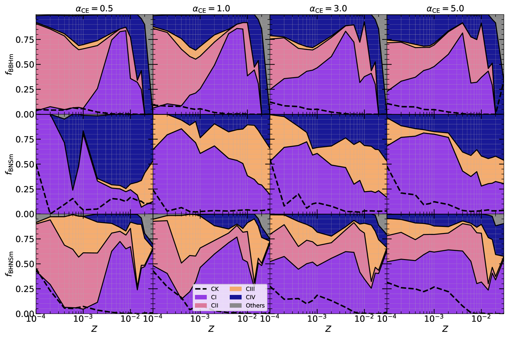
Figure 14: Relative fraction of systems produced through the four main formation channels (Section 4.2) as a function of the metallicity for BBHs (upper panels), BNSs (middle panels) and BHNSs (lower panels) that merge within 14 Gyr in our fiducial model (Section 3.2). The panels in each column refer to a different value of the CE efficiency parameter, $\alpha_{\mathrm{CE}}$, as reported in the titles (Section 2.3.3). The dashed lines indicate the fraction of systems that undergo at least one CE triggered by a collision at periastron (Section 2.3.5). The online repository () contains versions of this plot made for the alternative setup models, and alternative versions of this plot made considering the number of objects rather than the relative fractions.

Most merging BNSs in the fiducial model form through channel I ($\approx 59\%$). The other merging BNS progenitors evolve following formation channels III ($\approx 22\%$) and IV ($\approx 18\%$). In agreement with previous studies (e.g., Giacobbo & Mapelli, 2018; Kruckow et al., 2018; Vigna-Gómez et al., 2018), we find that is not possible to produce BNS mergers just through stable mass transfer episodes (channel II).

Since CE evolution is crucial for the formation of BNSs (all the BNS progenitors undergo at least two CE episodes), the relative formation channel fraction strongly depends on the parameter $\alpha_{\mathrm{CE}}$ (Table 6 and Fig. 14).

Metallicity has a significant impact on the evolution of NS progenitors (see, e.g., the first two rows in Fig. 7). In particular, metal-poor stars tend to interact after core He burning, while metal-rich stars interact during the HG or giant-branch phase (Table 2). The stellar phase is important to distinguish between stable and unstable mass transfer. Moreover, stars with similar radii but in different evolution phases can have different envelope binding energy favouring or disfavouring CE ejection. As a consequence, the relative formation-channel fractions vary significantly with metallicity.

The least massive BNS progenitors evolve through channel I and channel III (see Fig. 15). Almost all these binaries ($99\%$) undergo an additional second CE episode when the pure-He secondary expands starting a new unstable RLO (case BB mass transfer, see e.g. Broekgaarden et al. 2021).

Most of the systems evolving through channel IV (97%) do not activate a double-core CE, rather they undergo a first stable RLO in which the primary star loses the H-rich envelope. Later on, the secondary star begins an unstable RLO and expels the H-rich envelope after CE. Before the first NS formation, in almost half of the systems, the primary star triggers an additional CE turning into a naked-CO star (unstable case BB mass transfer). After the first NS formation, the pure-He secondary star triggers an additional CE episode in 90% of the cases. The minority of binaries that undergo a double-core CE ($\approx 3\%$) contain either massive NS progenitors close to the NS/BH boundary ($\approx 20\ \mbox{M${}_{\odot}$}$) or light progenitors ($\approx 11\mbox{M${}_{\odot}$}$) in an initial wide configuration ($a_{\mathrm{ini}}\gtrsim 1000\ \mbox{R${}_{\odot}$}{}$).

The evolution of the NS progenitors along the HG phase plays an important role in all the three main formation channels, especially at intermediate/high metallicity. For $Z>0.001$, the first interaction between the secondary star and the already formed NS begins when the star expands during the HG phase (up to $300\ \mbox{R${}_{\odot}$}{}$, see Fig. 7). In the fiducial model, stars in the HG phase are always stable and the RLO mass transfer continues until the secondary star changes the bse stellar type. At that point, the mass transfer becomes unstable due to large secondary-to-NS mass ratio ($q\gtrsim 10$).

In the alternative model QCBSE (Table 3), all the secondary star–NS interactions during the HG phase lead to a direct merger. Therefore, the number of BNS progenitors decreases in all the formation channels, but the suppression is maximum for channels I and III (Fig. 16).

The model variations of the RBSE and QHE model (at low metallicity) reduce the possibility to start an interaction after the first stable mass transfer reducing the number of channel I BNSs (Fig. 16).

Larger natal kick (models K$\sigma$150 and K$\sigma$265) can easily break the binary after the first NS formation reducing the number of BNSs, except for the tightest ones produced through channel IV (Fig. 16).

Higher envelope binding energies (models LK and LC, see Appendix A.1.4) drastically reduce the number of BNSs for $\alpha_{\mathrm{CE}}<1$: such simulations do not produce merging BNSs except for a few peculiar systems at $Z>0.002$. Such systems, evolving through channel IV, trigger the first CE between a pure-He star and a partially stripped H-rich star, then they avoid any interactions after the first NS formation. The channel fractions in model LX are similar to the fiducial model for $\alpha_{\mathrm{CE}}>1$, and similar to the LK and LC models in the other cases.

The relative formation-channel fractions in the other models do not show significant differences with respect to the fiducial model.

Both Vigna-Gómez et al. (2018) and Kruckow et al. (2018) found that formation channel I still dominates ($\gtrsim 70\%$) at high metallicity ($Z=0.014$ and $Z=0.0088$, respectively). In Dominik et al. (2012), the channel I fraction (channel NSNS01 and NSNS03 in their Table 4) is $\approx 87\%$ at $Z=0.02$. In contrast, in all our tested models, the fraction of BNSs formed through channel I is always $\lesssim 50\%$ for $Z>0.008$. Interestingly, the models in which the fraction drops to $\approx 0$ are the most similar ones (QCBSE and RBSE) to the binary-evolution models by Vigna-Gómez et al. (2018) and Dominik et al. (2012).

This large discrepancy derives from two important differences: their optimistic (versus our pessimistic) assumption for CE during the HG phase, and the stellar evolution models. We test the optimistic assumption in the OPT model (Fig. 16), and find that only in the case of $\alpha_{\mathrm{CE}}=5$ the channel I fraction reaches $\approx 50\%$ at high metallicity. In all the other cases, channel I remains subdominant and its fraction even decreases for $\alpha_{\mathrm{CE}}\leq 1$. Therefore, we conclude that the stellar evolution is the main driver of the discrepancy between our channel fractions and those of Dominik et al. (2012) and Vigna-Gómez et al. (2018).

Both Dominik et al. (2012) and Vigna-Gómez et al. (2018) used bse-like codes (startrack and compas), so the difference between their stellar evolution model (based on Pols et al. 1998) and parsec can be appreciated in Fig. 7 (see also Section 3.1.1). In the mass range of NS progenitors, the bse-like stellar tracks do not show a strong dependence on metallicity and interact mostly after core He burning for $M_{\mathrm{ZAMS}}>12\ \mbox{M${}_{\odot}$}$. In contrast, the parsec stellar tracks are markedly different at different metallicity and most of the interactions at $Z>0.001$ are triggered during the HG phase leading directly to a merger in the case of unstable RLO. Even considering the optimistic CE model, the binding energies in the HG phase are so high (Appendix A.1.4) that most of the CEs end with a coalescence.

4.2.4 Formation channels of BHNS mergers

In the fiducial model (F) most BHNS mergers form through channel I ($\approx 51\%$), followed by channel II ($\approx 25\%$), III ($\approx 15\%$), and IV ($\approx 8\%$). Table 6 and Fig. 14 show that the relative formation-channel fraction remains almost constant for all the values of $\alpha_{\mathrm{CE}}$, in the whole metallicity range. The largest differences are found for low $\alpha_{\mathrm{CE}}$ values and low/intermediate metallicity, in which channels I and III are suppressed in favour of channel II, and at high metallicity where channel II drops to $\approx 0$% and channel III rises up to $\approx 30\mathrm{-}50\%$.

The most massive BHNS progenitors follow channel III producing the most massive merging BHNSs (Fig. 15). Compared to BBHs and BNSs, the contribution of channel IV decreases in the whole $\alpha_{\mathrm{CE}}$ and $Z$ range. This channel is populated by stars with similar ZAMS mass evolving almost synchronously (see Sections 4.2.2 and 4.2.3). In the case of BHNS progenitors, this means selecting peculiar systems in a small mass range close to the NS/BH mass boundary ($\approx 22\ \mbox{M${}_{\odot}$}$, see Fig. 15). Half of the systems trigger a double-core CE in the late evolutionary phases (sevn phase 5 or 6, see Table 2). The other systems have an initial tighter configuration ($a_{\mathrm{ini}}\approx 50\mathrm{-}200\ \mbox{R${}_{\odot}$}$) and pass through an episode of stable mass transfer before triggering the first CE.

Figure 16 shows that the variation of simulation parameters does not have a strong impact in the relative channel fraction of merging BHNSs. The most relevant differences are present in the model LK (for low $\alpha_{\mathrm{CE}}$ values), in which the higher binding energies (Appendix A.1.4) totally suppress channels III and IV.

The results of all our simulations do not agree with the recent results by Broekgaarden et al. (2021), in which almost all the merging BHNSs are formed through channel I ($86\%$) and only $8\%$ of the progenitors evolve through channel II ($4\%$) and III ($4\%$). In their work, the relative fractions refer to the systems that are detectable by LIGO and Virgo, so they are biased toward binaries with high metallicity ($Z\gtrsim 0.008$) hosting massive BHs. In their simulations, such systems form preferentially through channel I. In our case, instead, the same “selection effects” should boost the percentage of channel III BHNSs, increasing even more the discrepancy (Figs. 14 and 15). Similarly, our results do not agree with Dominik et al. (2012) in which 97% of the merging BHNSs belong to channel I at $Z=0.02$, while at $Z=0.002$ the channel I fraction decreases to 25%, and most of the merging BHNSs ($\approx 67\%$) form through channels III and IV. Since the overall number of merging BHNSs in Broekgaarden et al. (2021) is comparable with our results (Fig. 17 and Section 4.3.3), we conclude that the differences are mostly driven by the different stellar evolution models (both Dominik et al. 2012 and Broekgaarden et al. 2021 use bse-like code based on the Pols et al. 1998 stellar tracks).

Our results are similar to what found by Kruckow et al. (2018). Assuming $\alpha_{\mathrm{CE}}=0.5$ and $Z=0.0088$, they estimate that $\approx 79\%$ of the merging BHNS belong to channel I, while the remaining systems evolve through channel II ($\approx 19\%$). The fraction of merging BHNSs evolving through stable mass transfers (channel II) is consistent with our results for $\alpha_{\mathrm{CE}}=0.5$, but we find that a non-negligible fraction of merging BHNSs ($\approx 20\%$) evolve through the CE channels III and IV. The cause of such difference is the larger binding energy of stellar envelopes used in combine (Appendix C). In our simulation model with the highest envelope binding energy (LK, see Appendix A.1.4) and $\alpha_{\mathrm{CE}}\leq 1$, the merging BHNSs form solely through channel I ($\approx 90\%$) and II ($\approx 10\%$) at $0.004\leq Z\leq 0.01$ (Fig. 16).

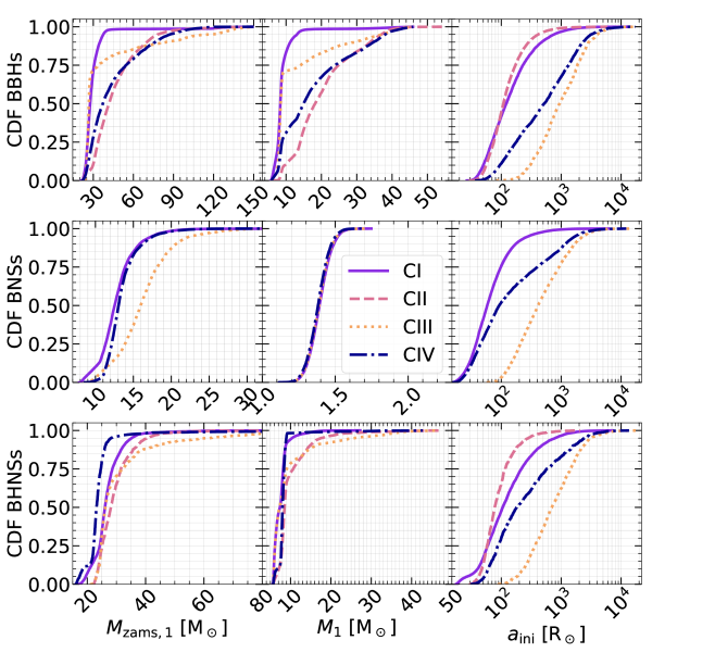
Figure 15: Cumulative distribution function for a sample of properties (left-hand column: ZAMS mass of the primary star; middle column: mass of the primary compact remnant; right-hand column: initial semi-major axis of BBHs (upper row), BNSs (central rows) and BHNSs (lower row) that merge within 14 Gyr in the fiducial model (Section 3.2). The primary is always the most massive object in the binary. Due to binary interactions, the primary compact remnant can be produced by the secondary star and vice-versa. For each BCO population, we consider all the sampled $\alpha_{\mathrm{CE}}$ and $Z$ values (Section 3.3). The different lines indicate the four main formation channels (Section 4.2): I (violet solid), II (pink dashed), III (orange dotted), and IV (blue dot-dashed line). The versions of this plot made for the alternative setup models can be found in the online repository ().

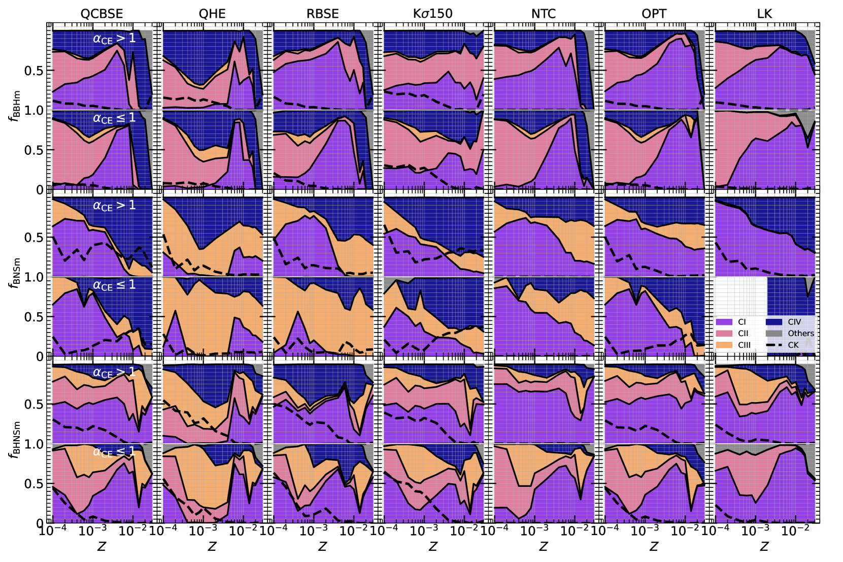
Figure 16: Same as Fig. 14, but showing the relative formation-channel fraction for different models as indicated in the titles (see Table 5 and Section 3.2). In each panel, the bottom part of the plot shows the channel fractions considering all the merging BCOs from the simulations with low-$\alpha_{\mathrm{CE}}$ values (0.5, 1), while the top part shows the results considering all the simulations with high-$\alpha_{\mathrm{CE}}$ values (3, 5). The lack of merging BNSs in the LK simulations for $\alpha_{\mathrm{CE}}\leq 1$ produces the white empty region in the corresponding panel.

4.3 Merger efficiency

We define the merger ($\eta$) and formation ($\eta_{\mathrm{f}}$) efficiency as

$$\begin{split}\eta&=\frac{N_{\mathrm{BCO}}(t_{\mathrm{del}}<14\ \mathrm{Gyr})}{M_{\mathrm{pop}}}\\ \eta_{\mathrm{f}}&=\frac{N_{\mathrm{BCO}}}{M_{\mathrm{pop}}},\end{split}$$ (51)

where $N_{\mathrm{BCO}}$ is the number of BCOs, $M_{\mathrm{pop}}$ is the total mass of the simulated stellar population, and $t_{\mathrm{del}}$ is the delay time, i.e. the time elapsed from the beginning of the simulation to the BCO merger. We estimate $M_{\mathrm{pop}}$ including the correction for the incomplete sample of the IMF (see Section 3.3), and assuming that half of the population mass is stored in binaries.

Figure 17 shows $\eta_{\mathrm{f}}$ and $\eta$ as a function of metallicity for BBHs, BNSs and BHNSs in our fiducial model. Figure 17 also compares our results with the merger efficiency found by Spera et al. (2019) using the previous version of sevn (assuming $\alpha_{\mathrm{CE}}=1$ and $\lambda_{\mathrm{CE}}=0.1$), Giacobbo & Mapelli (2020) using mobse ($\alpha_{\mathrm{CE}}=5$ and $\lambda_{\mathrm{CE}}$ prescriptions by Claeys et al. 2014), and Broekgaarden et al. (2022) using COMPAS ($\alpha_{\mathrm{CE}}=1$ and $\lambda_{\mathrm{CE}}$ prescriptions by Xu & Li 2010b). In Fig. 18, we compare the BBH merger efficiency of the default model with some of the alternative models. Figs. 19 and 20 show the same comparison for BNSs and BHNSs.

4.3.1 BBH merger efficiency

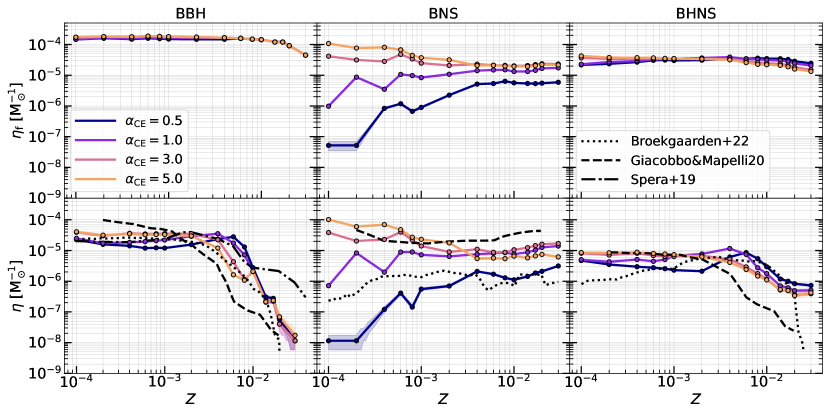
Figure 17: Formation ($\eta_{\mathrm{f}}$) and merger ($\eta$) efficiency for BBHs (left-hand panels), BNSs (middle panels) and BHNSs (right-hand panels) as a function of metallicity for the fiducial model (see Section 3.2). The total simulated mass has been corrected for the binary fraction (assumed 0.5) and for the partial sampling of the IMF (Section 3.3). The line colours show the results obtained assuming different CE efficiency parameters $\alpha_{\mathrm{CE}}$ (Section 3.3). The shaded areas show the 0.16 and 0.84 percentiles obtained sampling from Poissonian distributions. The black lines show the merger efficiency by other authors: Broekgaarden et al. (2022) (model A, dotted), Giacobbo & Mapelli (2020) (model Ej1, dashed), Spera et al. (2019) (dot-dashed). The versions of this plot made for the alternative setup models can be found in the online repository ().

In the fiducial model, the formation efficiency of BBHs is almost constant at all metallicities and for all the sampled $\alpha_{\mathrm{CE}}$ ($\eta_{\mathrm{f}}\approx{10^{-4}}\ \mathrm{M}^{-1}_{\odot}$), while the merger efficiency decreases from a few $\times{}10^{-5}$ M_⊙ for $Z<0.002$ to $10^{-6}\mathrm{-}10^{-8}$ M_⊙ at high metallicity ($Z>0.01$).

The differences between $\eta$ and $\eta_{\mathrm{f}}$ depend on the different dominant formation channels for BBHs and merging BBHs. Most BBH progenitors ($>70\%$) do not interact or interact only via stable mass transfer episodes, hence their final separation is too large ($>100\ \mbox{R${}_{\odot}$}{}$) to make them merge in an Hubble time.

The increasing importance of stellar winds at high metallicity reduces $\eta$ for $Z\gtrsim 0.008$. In fact, stars losing a significant amount of mass during the evolution remain more compact (see, e.g., Fig. 7), reducing binary interactions, and produce less massive BHs increasing the BBH merger time (Figs. 8 and 12). Figure 17 shows that CE efficiency has a much lower impact on the merger efficiency with respect to the metallicity. The largest differences are at intermediate metallicities ($0.008<Z<0.004$), where almost 90% of the BBH progenitors undergo at least one CE episode.

For $Z<0.01$ our results are in agreement with Spera et al. (2019), especially for $\alpha_{\mathrm{CE}}=1$. At higher metallicity, the simulations by Spera et al. (2019) produce a significantly larger number of BBH mergers. This happens because Spera et al. (2019) adopt a constant value $\lambda_{\mathrm{CE}}=0.1$, resulting in high binding energies. Higher binding energies combined with low $\alpha_{\mathrm{CE}}$ values let more massive binaries produce tight BBHs through channel I. We find similar results using the LC model in which we also set $\lambda_{\mathrm{CE}}=0.1$ (Fig. 18).

The BBH merger efficiency by Giacobbo & Mapelli (2020) shows a more steep gradient as a function of metallicity. At low metallicity, our simulations produce less BBHs by a factor 3–6. From $Z=0.002$ onward, our BBH merger efficiency becomes 10–100 times larger than what estimated by Giacobbo & Mapelli (2020). This trend is present in all our models (Fig. 18). Therefore, this difference mostly springs from the different stellar evolution model.

Our fiducial model with $\alpha_{\mathrm{CE}}>1$ shows a good agreement with the $\eta$ estimated by Broekgaarden et al. (2022). However, the two models are based on many different assumptions (e.g., different values for $\alpha_{\mathrm{CE}}$ and $\lambda_{\mathrm{CE}}$, different assumptions on the mass transfer stability). This comparison highlights how the effects of binary and stellar evolution are highly degenerate.

The merger efficiency drops by up to a factor of 10 in the models QHE, K$\sigma$150 and K$\sigma$265. In QHE, the smaller radius of the secondary star reduces the chance of starting a binary interaction, while the high supernova kicks in the other two models break a large number of binaries. The differences are less evident at high-metallicity, where the quasi-homogeneous evolution is switched off and most BBH mergers form through peculiar evolution routes (e.g., channel IV or lucky kicks).

Models LX, LC and LK produce a dramatic increment of BBH mergers at high metallicity, because of their high binding energies. Merging BBHs at low metallicity ($Z\leq{}0.001$) form mainly through channel II (stable mass transfer) so their number is not significantly affected by changes in the envelope binding energy. Finally, the OPT model produces a factor of 2–10 more BBHs at intermediate and high metallicity.

4.3.2 BNS merger efficiency

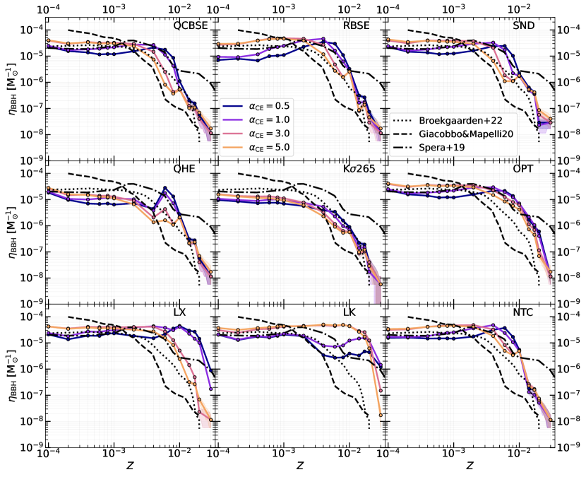
Figure 18: Same as Fig. 17, but showing only the BBH merger efficiency for a selection of further simulation models as reported by the labels in the top-right corner of each panel (Section 3.2 and Table 5).

Given the low NS mass ($\approx 1.33\ \mbox{M${}_{\odot}$}$), the only way for BNS progenitors to survive to supernova kicks is through CE episodes that shrink the semi-major axis and remove the stellar envelope producing low effective supernova kicks (Section 2.2.4). Therefore, most of the formed BNSs are tight enough to merge within an Hubble time. As a consequence, the BNS formation and merger efficiency are similar, with the only exception of case $\alpha_{\rm CE}=0.5$ at low metallicity (Fig. 17).

Since the formation of BNSs passes though at least one CE episode, their merger efficiency significantly depends on $\alpha_{\mathrm{CE}}$, as already found in other works (see,e. g. Vigna-Gómez et al., 2018; Giacobbo & Mapelli, 2020; Santoliquido et al., 2021; Broekgaarden et al., 2022). The trend of $\eta$ with progenitor’s metallicity also depends on the envelope binding energy, which is higher for lower metallicity in our models (Appendix A.1.4). For $\alpha_{\rm CE}=0.5$, we find the largest dependence of $\eta$ on progenitor’s metallicity: $\eta$ decreases by 4 orders of magnitude from high to low metallicity. The formation of BNSs is suppressed at low $Z$ and for $\alpha_{\mathrm{CE}}\leq{}1$, because most CEs end with a premature coalescence. Vice versa, for $\alpha_{\rm CE}\geq{}3$, $\eta$ decreases as the metallicity increases, because larger values of $\alpha_{\rm CE}$ combined with lower binding energies produce wider post-CE systems.

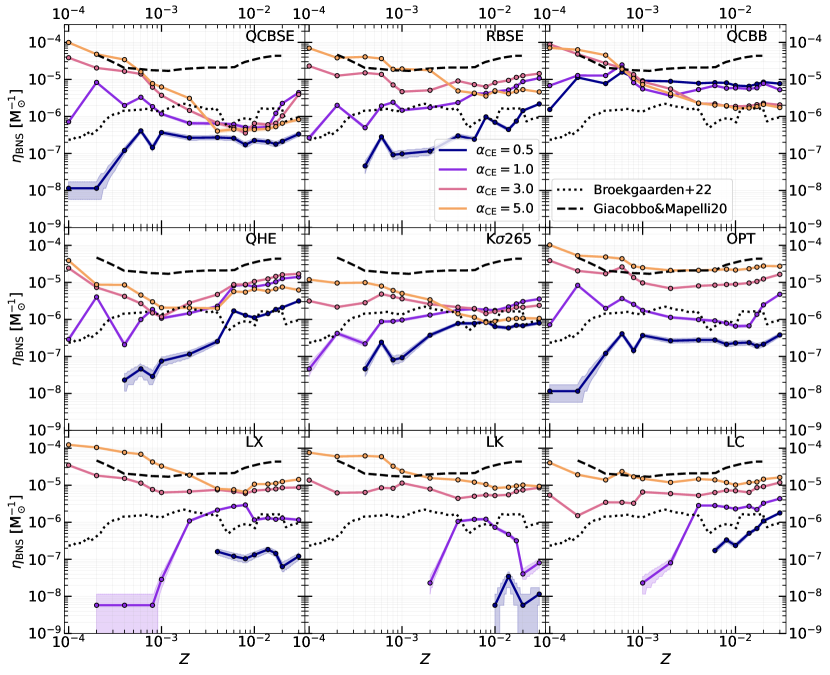
Figure 19: BNS merger efficiency for a selection of simulation models as specified by the labels in the top-right corner of each panel (Section 3.2 and Table 5). Different colours refer to values of $\alpha_{\rm CE}=0.5,$ 1, 3, 5. The dotted and dashed black lines show the results by Broekgaarden et al. (2022) and Giacobbo & Mapelli (2020), respectively.

The merger efficiency by Giacobbo & Mapelli (2020) shows a flatter metallicity trend for $\mbox{$\alpha_{\mathrm{CE}}$}=5$, while the one by Broekgaarden et al. (2022) is scaled-down by a factor of $\approx{10}$ with respect to our result (assuming $\mbox{$\alpha_{\mathrm{CE}}$}=1$).

Figure 19 shows that most of the runs alternative to our fiducial model produce a decrease of the BNS merger efficiency. In particular, the enhanced binding energy in models LX, LK, and LC reduces $\eta$ at low/intermediate metallicities, especially for models with $\alpha_{\mathrm{CE}}\leq 1$ for which the formation of BNSs is highly suppressed.

QCBSE, OPT and QCBB are the most interesting models, since these assume the same mass transfer stability criteria that are usually adopted in bse-like codes (see, e.g. Vigna-Gómez et al., 2018; Giacobbo & Mapelli, 2020). The model QCBSE produces a steep metallicity gradient. The presence of a metallicity gradient in the merger efficiency has a strong impact on the cosmological evolution of the merger rate density (Section 4.4). In the OPT model, we also use the QCBSE option for mass transfer stability; the optimistic CE assumption allows many more systems to survive the CE at high metallicity.

In model QCBB, mass transfer is always stable if the donor is a pure-He star (case BB mass transfer, see e.g., Vigna-Gómez et al. 2018). In simulations with $\alpha_{\mathrm{CE}}>1$, the configuration of the binaries after the case BB mass transfer is often too wide to produce a merging BNS. Hence, the merger efficiency decreases, especially at high metallicity. In contrast, for lower $\alpha_{\mathrm{CE}}$, the BNS progenitors are already in a tight configuration before the case BB mass transfer. Avoiding the last CE episode, most of the systems that coalesce in the fiducial model are now able to produce a merging BNS. As a consequence, $\eta$ increases and becomes almost independent of the metallicity.

4.3.3 BHNS merger efficiency

The formation and merger efficiency of BHNSs is similar to BBHs, although the merger efficiency has a milder dependence on metallicity. At $Z>0.004$, $\eta$ decreases by one order of magnitude and flattens at $Z>0.01$. The minimum value of $\eta$ corresponds to the metallicity for which we observe a suppression of channel I (Fig. 14).

At low metallicity our results agree with the BHNS merger efficiency estimated by Giacobbo & Mapelli (2020), but, similarly to the case of BBHs, their $\eta$ shows a much steeper trend wih metallicity. The results by Broekgaarden et al. (2022) are qualitatively in agreement with our results (within a factor of 2–4). Our results and those by Broekgaarden et al. (2022) disagree only at very high metallicity ($Z>0.02$), where our models substantially differ with respect to the Pols et al. (1998) tracks used in bse-like codes.

As for the other BCOs, the QHE model and the models predicting larger natal kicks reduce the total number of BHNS mergers up to a factor of 10. The models with higher binding energies (LX, LK and LC) allow more metal-rich binaries to shrink enough during CE, increasing the number of merging BHNSs at $Z>0.01$. For low $\alpha_{\mathrm{CE}}$ values, the significant boost of BHNS mergers at high metallicity produces a rising $\eta$ profile as a function of metallicity.

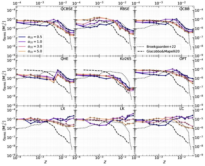
Figure 20: Same as Fig. 19 but for BHNSs.

4.4 Merger rate density

We estimate the evolution of BCO mergers with redshift by convolving the outputs of sevn with our semi-analytic code Cosmo$\mathcal{R}$ate (Santoliquido et al., 2020; Santoliquido et al., 2021). Cosmo$\mathcal{R}$ate estimates the merger rate density of compact objects as

$$\mathcal{R}(z)=\int_{z_{{\rm{max}}}}^{z}\left[\int_{Z_{{\rm{min}}}}^{Z_{{\rm{max}}}}{\rm{SFRD}}(z^{\prime},Z)\,{}\mathcal{F}(z^{\prime},z,Z)\,{}{\rm{d}}Z\right]\,{}\frac{{{\rm d}t(z^{\prime})}}{{\rm{d}}z^{\prime}}\,{}{\rm{d}}z^{\prime},$$ (52)

where

$$\frac{{\rm{d}}t(z^{\prime})}{{\rm{d}}z^{\prime}}=[H_{0}\,{}(1+z^{\prime})]^{-1}\,{}[(1+z^{\prime})^{3}\Omega_{M}+\Omega_{\Lambda}]^{-1/2}.$$ (53)

In the above equation, $H_{0}$ is the Hubble constant, $\Omega_{M}$ and $\Omega_{\Lambda}$ are the matter and energy density, respectively. We adopt the values in Aghanim et al. (2020). The term $\mathcal{F}(z^{\prime},z,Z)$ is given by:

$$\mathcal{F}(z^{\prime},z,Z)=\frac{1}{M_{{\rm{pop}}}(Z)}\frac{{\rm{d}}\mathcal{N}(z^{\prime},z,Z)}{{\rm{d}}t(z)},$$ (54)

where $M_{{\rm{pop}}}(Z)$ is the total initial mass of the simulated stellar population (including the correction for the incomplete sample of the IMF, and for the binary fraction), and ${{\rm{d}}\mathcal{N}(z^{\prime},z,Z)/{\rm{d}}}t(z)$ is the rate of binary compact object mergers forming from stars with initial metallicity $Z$ at redshift $z^{\prime}$ and merging at $z$, extracted from our sevn catalogues. In Cosmo$\mathcal{R}$ate, ${\rm{SFRD}}(z,Z)$ is given by

$${\rm{SFRD}}(z^{\prime},Z)=\psi(z^{\prime})\,{}p(z^{\prime},Z),$$ (55)

where $\psi(z^{\prime})$ is the cosmic SFR density at formation redshift $z^{\prime}$, and $p(z^{\prime},Z)$ is the log-normal distribution of metallicities $Z$ at fixed formation redshift $z^{\prime}$, with average $\mu(z^{\prime})$ and spread $\sigma_{Z}$. Here, we take both $\psi{}(z)$ and $\mu{}(z)$ from Madau & Fragos (2017). Finally, we assume a metallicity spread $\sigma_{Z}=0.2$.

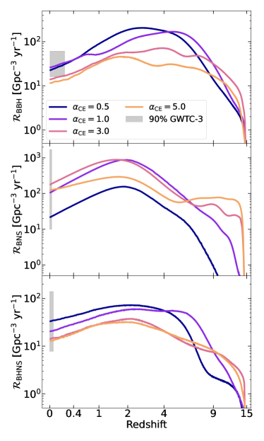
Figure 21: Merger rate density evolution of BBHs (top), BNSs (middle), and BHNSs (bottom), in the fiducial model (F), as a function of redshift. The line colours refer to simulations with different $\alpha_{\mathrm{CE}}$ values as reported in the legend. The grey shaded area shows the most conservative 90% credible intervals of the local merger rate density inferred from GWTC-3 (Abbott et al., 2023). The width of the shaded areas indicates the instrumental horizon obtained by assuming BBHs, BNSs and BHNSs of mass (30, 30), (10, 1.4), and (1.4, 1.4) M_⊙, respectively. Alternative versions of this plot referring to the alternative models and alternative metallicity spreads, $\sigma_{\mathrm{Z}}$ (see main text) can be found in the gitlab repository of the paper ().

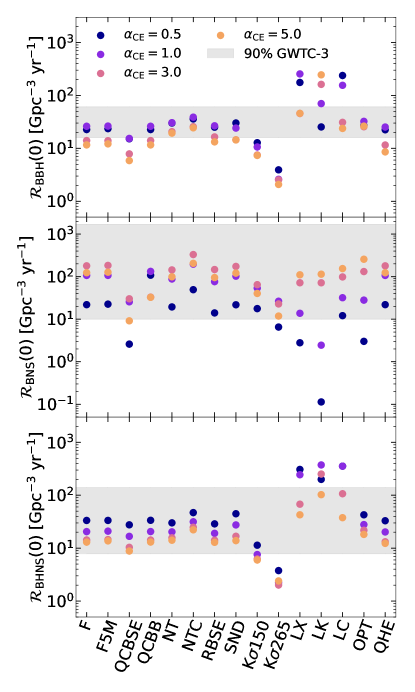
Figure 22: Merger rate density in the local Universe ($z=0$) of BBHs (top), BNSs (middle), and BHNSs (bottom) for a sub-sample of models (Table 5). Each colour indicates the results of a different $\alpha_{\mathrm{CE}}$ value. The gray shaded area shows the most conservative 90% credible intervals inferred from GWTC-3 (Abbott et al., 2023). Other versions of this plot referring to alternative metallicity spreads $\sigma_{\mathrm{Z}}$ (see main text) can be found in the gitlab repository of the paper ().

Figure 21 shows the merger rate density in the comoving frame of BBHs, BNSs, and BHNSs, according to our fiducial model, for the four considered values of $\alpha_{\rm CE}$. For all the considered models, the merger rate density increases as a function of redshift, up to $z\sim{2}$ (or an even higher redshift in the case of BBHs and BHNSs).

The merger rate density of BNSs has a peak for $z\leq{}2$, consistent with the peak of the star formation rate density ($z\approx{2}$, Madau & Dickinson 2014) convolved with a short delay time. In contrast, the merger rate density of BHNSs and BBHs peaks at $z>2$, because of the combined effect of star formation rate and metallicity dependence.

The choice of the $\alpha_{\rm CE}$ parameter affects the merger rate density, with an impact of a factor of 10 for BNSs (up to 3 for BHNSs and BBHs).

The results of our fiducial model are within the 90% credible interval inferred by the LVK after the third observing run (Abbott et al., 2023) for $\mbox{$\alpha_{\mathrm{CE}}$}\leq 1$ for BBHs and for all the considered values of $\alpha_{\mathrm{CE}}$ for BNSs and BHNSs. Here, we assumed a metallicity spread $\sigma_{\rm Z}=0.2$ which maximises this agreement. For larger metallicity spreads, the models tend to overproduce the merger rate density of BBHs, as already shown by Santoliquido et al. (2022).

Figure 22 compares the local ($z=0$) merger rate density of several different models run in this work. We find a factor of 100 difference among different models considered here. In particular, large natal kicks (K$\sigma$265) are associated with the lowest merger rate densities for BBHs and BHNSs.

As already discussed in Section 4.3.2, the combination of the parsec stellar models with the standard criterion for the stability of the mass transfer (QCBSE, see Table 3) drastically reduces the number of BNSs at high metallicity. As a consequence, the model QCBSE produces the lowest local BNS merger rate density.

The models LX, LK, and LC are associated with the highest local merger rate of BBHs and BHNSs, and the lowest merger rate of BNSs. In fact, the higher binding energies in such models allow more systems to shrink enough to produce merging BBHs and BHNSs. In contrast, BNS progenitors undergo multiple CE episodes and have a lower reservoir of binding energy, on average; hence they tend to coalesce during CE, especially for ow $\alpha_{\mathrm{CE}}$values.

In most models with $\sigma_{\rm Z}=0.2$, the local merger rate density of BBHs and BHNSs is $\approx{2-50}$ Gpc^-3 yr^-1, while the BNS merger rate density spans from $\approx{3}$ to $\approx{400}$ Gpc^-3 yr^-1. Here, we show the results for a fixed value of the median metallicity and metallicity spread of the Universe: the merger rate density of BBHs and BHNSs are extremely sensitive to this choice (e.g., Chruslinska et al., 2019; Boco et al., 2019; Bouffanais et al., 2021b; Broekgaarden et al., 2022; Santoliquido et al., 2022).

5 Discussion

5.1 Impact of stellar evolution on BCO properties

In Section 3.1.1, we highlighted the differences between the parsec stellar tracks used in this work and the ones implemented in bse-like codes (Pols et al., 1998). The largest discrepancies are at high metallicity and/or for high-mass stars (e.g., Fig. 7). Agrawal et al. (2020) showed that different stellar evolution models can significantly influence the mass spectrum of BHs evolved in isolation (see also Klencki et al., 2020). In addition, many authors pointed out that the uncertainties in stellar evolution can have a dramatic impact on the mass range in which a star undergoes pair instability (e.g., Fields et al., 2018; Mapelli et al., 2020; Farmer et al., 2020; Costa et al., 2021; Vink et al., 2021).

In Section 4.1.1 (Fig. 8), we showed that several parsec stellar tracks do not have a monotonic increase of the core mass as a function of the ZAMS mass due to late dredge-up episodes Costa et al. (2021). As a consequence, massive metal-poor stars can avoid PPI ($M_{\mathrm{ZAMS}}\approx 100\ \mbox{M${}_{\odot}$}$) or PISN ($M_{\mathrm{ZAMS}}\approx 150\ \mbox{M${}_{\odot}$}$) producing massive BHs (up to $\approx 100\ \mbox{M${}_{\odot}$}{}$), well within the claimed pair instability mass gap (Fig. 12). Although such massive BHs cannot merge within an Hubble time via isolated binary evolution (Fig. 13 and Section 4.1.2), they can have an important role in the formation of massive BCO mergers in dynamically active stellar clusters (see e.g. Rastello et al., 2019; Di Carlo et al., 2020a; Rastello et al., 2020; Arca-Sedda et al., 2021b; Mapelli et al., 2021; Rastello et al., 2021).

In Section 4, we show that the details of stellar evolution play a fundamental role even during binary evolution, significantly affecting the properties of BCO mergers. In particular, using the parsec stellar tracks, we find that the “classic” formation channel of BCO mergers (channel I, see Section 4.2) can be strongly suppressed especially at high metallicity (Fig. 14).

Concerning the merger efficiency, the variations due to differences in the assumed stellar model have an impact as large as that of binary evolution uncertainties (e.g., efficiency of CE, supernova kicks; see, e.g., Giacobbo & Mapelli, 2020; Santoliquido et al., 2021; Broekgaarden et al., 2022).

Interestingly, the models for which we find the largest discrepancies on the formation channel and merger efficiency (especially regarding the BNSs) with respect to the results of bse-like codes are the ones with the most similar assumptions about binary evolution. For example, assuming the QCBSE stability criterion (Table 3), we obtain a steep metallicity trend for the BNS merger efficiency rather than the almost flat profile usually found in works adopting bse-like codes (Fig. 19). This implies that the main parameters describing binary evolution and the underlying stellar evolution models are highly correlated. Therefore, any attempt to constrain binary evolution parameters by comparing observations and population-synthesis results could be affected by a selection bias of the parameter space.

Our results point out that the investigation of the systematics and uncertainties in stellar evolution are fundamental for the analysis of the properties BCOs and for the astrophysical interpretation of the results obtained by the LVK.

The sevn code is designed to explore the parameter space. In fact, it allows to easily test different stellar evolution models using the same exact framework for binary evolution. In future works, we aim to exploit sevn to make a more comprehensive comparison of the state-of-the-art stellar evolution models.

5.2 About CE

In Section 4, we showed that the parameters related to CE, i.e. $\lambda_{\mathrm{CE}}$ for the envelope binding energy and $\alpha_{\mathrm{CE}}$ for CE efficiency have a large impact on the formation of merging BCOs, as already highlighted in many other works (e.g., Dominik et al., 2012; Vigna-Gómez et al., 2018; Giacobbo & Mapelli, 2018; Kruckow et al., 2018; Giacobbo & Mapelli, 2020; Klencki et al., 2021; Broekgaarden et al., 2021, 2022; Vigna-Gómez et al., 2022). Recent works suggest that the models used in binary population synthesis codes may be optimistic regarding CE survival, especially for massive stars (see, e.g., Klencki et al., 2021, 2022). As a consequence, these codes may overestimate the number of merging BBHs formed through CE (e.g., Briel et al., 2023; Marchant et al., 2021; Gallegos-Garcia et al., 2021). However, we found that the increase of the binding energy does not always decrease the number of BCO mergers (Section 4.2.2). Rather, it allows more (massive) systems to evolve through channel I (Fig. 16, see also Kruckow et al. 2016). At high metallicity, higher binding energies boost the merger efficiency and the merger rate of BBHs and BHNSs (Figs. 18 and 22), allowing the formation of more massive merging BBHs, also influencing the BH mass spectrum (Fig. 13).

Variations of $\alpha_{\mathrm{CE}}$ produce a scatter in the local merger rate density of BNSs up to one order of magnitude. In general, for $\mbox{$\alpha_{\mathrm{CE}}$}<1$, the predicted merger rates are just marginally consistent with the one found by the LVK after the third observing run (Abbott et al., 2023). For BBHs, low $\alpha_{\mathrm{CE}}$ values produce a larger number of mergers. A significant increase in the number of BBH mergers could result in a tension with the local merger rate estimated from GWTC-3 (Abbott et al., 2023) when also the contribution of other formation channels are taken into account (e.g. dynamical formation channel in star clusters).

In contrast, in the lower mass range of WD binaries, low $\alpha_{\mathrm{CE}}$ values seem to be the best match to the observed properties of post-CE MS–WD systems (e.g., Zorotovic et al., 2010; De Marco et al., 2011; Toonen & Nelemans, 2013; Camacho et al., 2014).

In conclusion, the $\alpha_{\mathrm{CE}}$$\lambda_{\mathrm{CE}}$ model often used in population synthesis codes (but see, e.g., Kruckow et al. 2018 and Korol et al. 2022 for alternative models) could be too simplistic to catch the complex physics of CE evolution, especially if we assume a constant value for $\alpha_{\mathrm{CE}}$ throughout the entire stellar mass range.

Recently, there have been many efforts to improve the models of CE (e.g., Halabi et al., 2018; Fragos et al., 2019; Law-Smith et al., 2020; Ragoler et al., 2022; Hirai & Mandel, 2022; Trani et al., 2022; Vigna-Gómez et al., 2022; Di Stefano et al., 2023). In the future, we aim to include and test additional CE models in sevn.

5.3 Other binary evolution processes

Aside from CE, the parameters that have a large impact on the formation and merger of BCOs are the ones regarding supernova kicks and stability of mass transfer. As expected, large natal kicks reduce the number of merging BCOs and alter their mass spectrum selecting preferentially massive binaries (Fig. 13).

The mass transfer stability criterion is the one that mostly correlates with the choice of the stellar evolution model. The combination of the parsec stellar tracks with the standard stability criterion used in bse-like codes (QCBSE, Table 3) produces a suppression of BCO merger efficiency, especially for BNSs (Fig. 19). Combining the model QCBSE with the optimistic CE assumption (model OPT) and large $\alpha_{\mathrm{CE}}$values ($>1$), brings back the efficiency of BCO mergers to the level of the fiducial model.

The quasi-homogeneous evolution reduces binary interactions, suppressing the number of BCO mergers at low metallicity (Figs. 18, 19, 20), but is thought to be ineffective at high metallicity ($Z>0.004$). As a consequence it only has a modest impact onto the local merger rate density (Fig. 22).

The models in which we disable the stellar tides (NT and NTC) do not significantly alter the formation channels of BCOs, their merger efficiency and local merger rate density. However, Fig. 13 shows that models without tides (NT and NTC) produce a flatter mass spectrum for BHs in BBH mergers. These are important results since models of stellar tides depend on a large number of parameters and on properties that are not always available in stellar tracks (e.g., stellar rotation and eddy turnover time, Section 2.3.4). In addition, recent observations of binary stars seem to challenge the predictions of the classical tide formalism used in population-synthesis studies, especially regarding dynamic tides (Justesen & Albrecht, 2021; Marcussen & Albrecht, 2022). Similarly, all the other models we tested do not introduce significant differences in the merger efficiency and local merger rate density, but can alter the features of the mass spectrum of BHs in BCO mergers (see, e.g., the SND and RBSE model in Fig. 13).

5.4 Systematics and caveats

Recent work highlights the importance of using self-consistent binding energy for the adopted stellar-evolution models (see e.g. Kruckow et al., 2016; Marchant et al., 2021; Klencki et al., 2021). Here, we use binding energy prescriptions that were derived for other stellar models (Appendix A.1.4). However, the four different formalisms we tested cover a wide range of binding energies (up to three orders of magnitude), from low values (Claeys et al., 2014) to very high ones (Klencki et al., 2021). In a follow-up study (Sgalletta et al., in prep.), we will show the impact of adopting values of the binding energy calculated directly from our stellar-evolution tracks. We also aim to investigate the effect of the possible dependence of the envelope binding-energy on the adiabatic mass-loss during CE, as highlighted by Deloye & Taam (2010); Ge et al. (2010a); Ge et al. (2022).

Although we simulated a large number of binaries, some of the simulations produce just a few BCOs. In addition, we use the same set of binaries for all the simulations. In order to asses the possible systematic effects due either to low-number statistic or to the limited sampling of the initial conditions, we ran a simulation using the fiducial setup (Section 3.2) but with a different set of $5\times 10^{6}$ binaries. The results of these simulations are stored in the gitlab repository of the paper (). We do not find any significant differences with respect to the fiducial model, except for the merger efficiency in regions of the parameter space in which the simulations produce a low number of BCOs ($<10$). This happens for $\alpha_{\mathrm{CE}}=0.5$ and $Z=0.03$ for BBHs, and $Z<0.0004$ for BNSs. These differences are within the uncertainties expected for a Poissonian distribution.

6 Summary

We presented the new release of the binary population-synthesis code sevn. With respect to its previous versions, sevn has been deeply revised to improve its performance, and to guarantee more flexibility in modelling single and binary star evolution processes: sevn now implements multiple possible options for core-collapse supernovae, pair instability, RLO, CE, natal kicks, stellar tides, and circularisation. The new version of sevn is publicly available at this link https://gitlab.com/sevncodes/sevn.git, together with an user-guide.

sevn describes stellar evolution by interpolating a set of evolutionary tracks, instead of using the commonly adopted fitting formulas by Hurley et al. (2000). In the new version, we added a completely new set of stellar-evolution tracks run with parsec (Bressan et al., 2012; Costa et al., 2019) and the MIST tracks (Choi et al., 2016).

We used sevn to investigate the formation and properties of binary compact objects (BCOs) exploring a wide portion of the parameter space. In the following, we summarise the main results of our analysis.

• Stellar evolution plays a fundamental role in defining the properties of BCOs, such as their formation channels, merger efficiency and merger rate density. Our results, obtained using sevn with parsec tracks, show systematic differences with respect the results of bse-like codes that are as large as (or even larger than) the effect of the uncertainties on binary-evolution processes (e.g., CE and natal kicks).

• We find that there is a degeneracy between the effects of binary-evolution parameters and stellar-evolution models. For example, the classical bse-like stability criterion applied to the parsec tracks induces a strong suppression (more than one order of magnitude) of the BNS merger rate with respect to the results of bse-like codes.

• Combining the parsec stellar tracks with the recent pair-instability prescriptions by Farmer et al. (2019) and Mapelli et al. (2020), it is possible to produce massive BHs (up to $\approx{100}\ \mbox{M${}_{\odot}$}$), well within the boundaries of the claimed pair-instability mass gap, just through single star evolution. However, the maximum mass of BHs in BBH mergers is $\approx{55}\ \mbox{M${}_{\odot}$}{}$ in all our runs. BHs more massive than $\approx{55}$ M_⊙ can still merge within the Hubble time, but only if they pair up dynamically with other BHs in dense star clusters and galactic nuclei.

• In our simulations, the importance of channel I for BCO formation (i.e., only stable mass transfer before the first compact remnant formation and then a CE episode) is strongly suppressed with respect to the large majority of the other works in the literature. In particular, at high metallicity ($Z\gtrsim{0.01}$) only less than $20\%$ of the merging BBHs and BNSs form via this channel, while other authors found fractions larger than $70\%$ ( e.g., Dominik et al., 2012; Giacobbo et al., 2018; Kruckow et al., 2018; Vigna-Gómez et al., 2018).

• The details of binary circularisation due to stellar tides do not seem to play an important role for the formation of BCOs. In particular, we obtain very similar results both using the detailed stellar tides formalism by Hurley et al. (2002) and a simpler model in which the binary is circularised at periastron at the onset of RLO.

• The local merger rate density of our fiducial models (10–30 Gpc^-3yr^-1 for BBHs, 20–200 Gpc^-3yr^-1 for BNSs, and 10–40 Gpc^-3yr^-1 for BHNSs) is consistent with the most recent estimates by the LVK (GWTC-3, Abbott et al. 2023). In contrast, the models for which the parameters of binary evolution are more similar to the default values of bse-like codes (e.g., Giacobbo & Mapelli, 2020; Santoliquido et al., 2021) show a significant tension with the credible intervals inferred by the LVK.

In conclusion, our work points out the need to include the uncertainties and systematics of stellar evolution in the investigation of the (already large) parameter space relevant for the formation, evolution and demography of BCOs. This is particularly important for the astrophysical interpretation of the results of current and forthcoming GW observatories. In this context, sevn represents an unique tool to deeply explore the parameter space of BCO formation.

Data Availability

All the data underlying this article are available in Zenodo at the link https://doi.org/10.5281/zenodo.7260770 (Version 2.0, Iorio et al., 2023). The codes used in this work are publicly available through gitlab repositories: sevn at https://gitlab.com/sevncodes/sevn.git (release Iorio22, https://gitlab.com/sevncodes/sevn/-/releases/iorio22), TrackCruncher at https://gitlab.com/sevncodes/trackcruncher.git, and pyblack at https://gitlab.com/iogiul/pyblack. All the Jupyter notebooks used to produce the plots in the paper are available in the gitlab repository https://gitlab.com/iogiul/iorio22_plot.git (release V3.0, https://gitlab.com/iogiul/iorio22_plot/-/releases/V3.0). The repository contains also additional plots not showed in this article. Each plot in the paper reports three icons pointing to specific path of the repository: specific folder containing the notebooks, the data and the images, Jupyter notebooks used to make the plot, direct link to the image.

Appendix A Additional features of sevn

A.1 Alternative to stellar-evolution tables

A.1.1 Core radius

The radii of the He and CO core, if not available in the stellar-evolution tables, are estimated as

$$R_{\mathrm{core}}=R_{0}\frac{1.1685M^{4.6}_{\mathrm{c}}}{M^{4}_{\mathrm{c}}+0.162M^{3}_{\mathrm{c}}+0.0065}\ \ \mbox{R${}_{\odot}$},$$ (56)

where $M_{\mathrm{c}}$ is the mass of the He or CO core in M_⊙, $R_{0}=0.1075$ for the He core and $R_{0}=0.0415$ for the CO core. The functional form of Eq. 56 is the same as used for the radius of naked helium stars in Eq. 78 of Hurley et al. (2000). We have adapted the coefficient and the normalisation to fit the radius of the He and CO cores in the parsec stellar tracks.

A.1.2 Inertia

sevn implements the following alternative options to estimate the stellar inertia.

• Eq. 109 from Hurley et al. (2000)

  $$I=0.1(M-M_{\mathrm{c}})R^{2}+0.21M_{\mathrm{c}}R^{2}_{\mathrm{c}};$$ (57)

• the formalism by de Mink et al. (2013)

  $$I=kM\,{}R^{2},$$ (58)

  where $k$ depends on the mass and radius of the star;

• the inertia of an homogeneous sphere

  $$I=\frac{2}{5}M\,{}R^{2};$$ (59)

• the inertia of an homogeneous hollow sphere (modelling the star’s envelope) plus an homogeneous sphere (modelling the core):

  $$I=\frac{2}{5}(M-M_{\mathrm{c}})\frac{R^{5}-R^{5}_{\mathrm{c}}}{R^{3}-R^{3}_{\mathrm{c}}}+\frac{2}{5}MR^{2}.$$ (60)

A.1.3 Convective envelope

The parsec tables also include the main properties of the convective envelope: the mass, radial extension and turnover timescale of the largest convective cells.

If these are not available, we estimate the mass and extension of the convective region following Section 7.1 of Hurley et al. (2000) and Eqs. 36–40 of Hurley et al. (2002). In practice, we assume that all the MS stars with $M_{\mathrm{ZAMS}}>1.25\ \mbox{M${}_{\odot}$}$ and all the pure-He stars have a radiative envelope. The MS stars with $M_{\mathrm{ZAMS}}\leq 1.25\ \mbox{M${}_{\odot}$}$ begin their evolution with a fully convective envelope that progressively recedes until the envelope is fully radiative at the end of the MS. Then, the process is reversed during the terminal-age MS phase (TAMS, sevn phase 2, see Table 2): the convective layers grow and the star becomes fully convective at the end of this phase.

The envelope of H-rich stars more evolved than the TAMS phase is assumed to be fully convective. Hurley et al. (2000) and Hurley et al. (2002) use the bse type 2 (HG) to set the transition to a fully convective envelope. There is not a direct correspondence between the bse type HG and the sevn phase TAMS, since it depends on the mass fraction of the convective envelope (Table 2), which is not known a priori if the tables are not used. As a consequence, in sevn the transition to a fully convective envelope could happen when the effective temperature of the star is still hot enough to be dominated by the radiative energy transport. We will improve this in future sevn versions; meanwhile we suggest to include the information about convection in the stellar-evolution tables when possible.

There are no analytic approximations for the turnover timescale: this is set to zero if the tables are not available. Therefore, processes that require this quantity have to implement their own alternative to the tables. For example, in the stellar tides (Section 2.3.4) the turnover timescale is estimated using Eq. 31 in Hurley et al. (2002) if it is not available in the tables.

A.1.4 Envelope binding energy

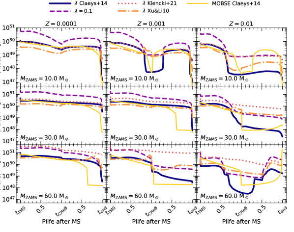
Figure 23: Evolution of the envelope binding energy during stellar evolution for a sample of stars with $M_{\mathrm{ZAMS}}=10$ (first row), 30 (second row), and $60\ \mbox{M${}_{\odot}$}{}$ (third row), and metallicity $Z=0.0001$ (first column), 0.001 (second column), 0.01 (third column). The x-axis indicates the percentage of life after the MS from the TAMS ($t_{\mathrm{TAMS}}$) up to the CHeB phase ($t_{\mathrm{CHeB}}$, see Table 2), and from the CHeB to the moment the star turns into a compact remnant or a pure-He star ($t_{\mathrm{end}}$). The gold solid thin line shows the binding energy of the mobse stellar models assuming the $\lambda_{\mathrm{CE}}$ formalism by Claeys et al. (2014). All the other lines show the binding energy of the parsec stellar models ($\lambda_{\mathrm{ov}}=0.5$, see Section 3.1) assuming different $\lambda_{\mathrm{CE}}$ prescriptions: blue solid line following Claeys et al. (2014), violet dashed line using $\lambda_{\mathrm{CE}}=0.1$, pink dotted line using the prescriptions by Klencki et al. (2021), orange dot-dashed line following Xu & Li (2010b). In all the cases, we estimate the binding energy maximising the fraction of internal and recombination energy (see the main text).

The envelope binding energy is a key quantity to determine the fate of a binary system during a CE phase (Section 2.3.3). The envelope loss during CE can be enhanced by taking into account the internal and recombination energy of the envelope (e.g., Lau et al., 2022), therefore the tables should contain the effective envelope binding energy, i.e. the gravitational binding energy reduced to take into account the aforementioned additional energy sources.

If the envelope binding energy tables are not available, sevn uses

$$E_{\mathrm{bind}}=-G\frac{MM_{\mathrm{env}}}{\lambda_{\mathrm{CE}}R}.$$ (61)

sevn implements the following options to calculate the parameter $\lambda_{\mathrm{CE}}$.

• Constant, $\lambda_{\mathrm{CE}}$ is set to a constant value. It is possible to set different $\lambda_{\mathrm{CE}}$ values for H-stars and pure-He stars.

• bse, $\lambda_{\mathrm{CE}}$ is estimated as in bse and mobse, i.e. adopting the formalism described by Claeys et al. (2014). Actually, this option of sevn is based on the most updated public version of bse and mobse, which differ from Appendix A of Claeys et al. (2014) for the following aspects. We replace Eq. A1 of Claeys et al. (2014) with the following equation:

  $$\lambda_{\mathrm{CE}}=\begin{cases}2\lambda_{2}~{}~{}~{}~{}~{}~{}~{}~{}~{}~{}~{}~{}~{}~{}~{}~{}~{}~{}~{}~{}~{}~{}~{}~{}~{}~{}~{}~{}~{}~{}~{}~{}~{}~{}~{}~{}~{}~{}~{}~{}~{}~{}~{}~{}~{}\mathrm{if}\ f_{\mathrm{conv}}=0\\ 2\lambda_{2}+f^{0.5}_{\mathrm{conv}}(\lambda_{1}-2\lambda_{2})~{}~{}~{}~{}~{}~{}~{}~{}~{}~{}~{}~{}~{}~{}~{}\mathrm{if}\ 0<f_{\mathrm{conv}}<1\\ \lambda_{1}~{}~{}~{}~{}~{}~{}~{}~{}~{}~{}~{}~{}~{}~{}~{}~{}~{}~{}~{}~{}~{}~{}~{}~{}~{}~{}~{}~{}~{}~{}~{}~{}~{}~{}~{}~{}~{}~{}~{}~{}~{}~{}~{}~{}~{}~{}~{}\mathrm{if}\ f_{\mathrm{conv}}\geq 1\end{cases},$$ (62)

  where $f_{\mathrm{conv}}$ is the mass fraction of the convective envelope with respect to the whole envelope. In addition, we replace the parameter $\lambda_{1}$ with $2\lambda_{1}$ in Eqs. A6 and A7 of Claeys et al. (2014). Claeys et al. (2014) introduced the parameter $\lambda_{\mathrm{ion}}\ \in\ [0,1]$ to parametrise the fraction of internal and recombination energy included in the estimate of the binding energy. We use $\lambda_{\mathrm{ion}}=1$ as default value. For pure-He stars, $\lambda_{\mathrm{CE}}=0.5$.

• Izzard04, same as the bse implementation, but in Eq. 62 we replace $f_{\mathrm{conv}}$ with the mass of the convective envelope expressed in solar units.

• Xu&Li10, we estimate $\lambda_{\mathrm{CE}}$ by interpolating on $M_{\mathrm{ZAMS}}$ the fitting equations by Xu & Li (2010a) and Xu & Li (2010b). Similar to the bse option, it is possible to set the fraction of internal and recombination energy, $\lambda_{\mathrm{ion}}$, to take into account the estimate of the effective binding energy. We use $\lambda_{\mathrm{ion}}=1$ as default value.

  For pure-He stars we use the formalism included in COMPAS:

  $$\lambda_{\mathrm{CE}}=0.3R^{-0.8}_{\mathrm{\lambda}},\ \mathrm{with}\ R_{\mathrm{\lambda}}=\min[120,\max[0.25,R]],$$ (63)

  where $R$ is the stellar radius expressed in solar units.

• Klencki21, we estimate $\lambda_{\mathrm{CE}}$ interpolating on $M_{\mathrm{ZAMS}}$ and $Z$ the fitting formulas by Klencki et al. (2021) calibrated on MESA tracks. Since Klencki et al. (2021) report only H-rich stars, we set $\lambda_{\mathrm{CE}}=0.5$ for pure-He stars.

We set to 0 the envelope binding energy for all the stars without a core (i.e., sevn phases 0, 1 for H-rich stars and phase 4 for pure-He stars), the naked-CO stars and the compact remnants.

In Fig. 23, we compare the binding energy estimated with different $\lambda_{\mathrm{CE}}$ prescriptions for the parsec stellar tracks. We also show the binding energy from mobse. From the TAMS to the ignition of the core He burning the binding energies from parsec and mobse (in both cases using the $\lambda_{\mathrm{CE}}$ prescription by Claeys et al. 2014) are qualitatively in agreement. In the later evolutionary phases the differences are more notable. The prescriptions by Klencki et al. (2021) and the constant $\lambda_{\mathrm{CE}}=0.1$ predict the largest binding energies, while the fitting formulas by Xu & Li (2010b) yield values of the binding energy that are generally intermediate between Claeys et al. (2014) and Klencki et al. (2021).

A.2 Electron-capture and core-collapse supernova models

sevn includes the following formalism for electron-capture and core-collapse supernovae (ECSN and CCSN, respectively).

• Rapid, rapid supernova model by Fryer et al. (2012).

• Delayed, delayed supernova model by Fryer et al. (2012). In both the delayed and the rapid model, the final mass depends on the total and CO-core mass of the star at the onset of core collapse. The mass of the compact remnant of an ECSN is equal to the pre-supernova CO-core mass.

• Rapid Gaussian, same as rapid, but the mass of the NSs (including NSs born from ECSNe) are drawn from a Gaussian distribution (see Section 2.2).

• Delayed Gaussian, same as delayed, but the mass of the NSs (including NSs born from ECSNe) are drawn from a Gaussian distribution (see Section 2.2).

• Compactness, supernova model based on the compactness parameter, defined as

  $$\xi_{\mathrm{2.5}}=\frac{2.5}{R(2.5\ \mbox{M${}_{\odot}$})/1000\,{}{\rm km}},$$ (64)

  i.e., as the ratio between a characteristic mass (2.5 M_⊙) and the radius (in units of 1000 km) enclosing this mass at the onset of the core collapse (O’Connor & Ott, 2011). In sevn, we estimate the compactness using Eq. 2 in Mapelli et al. (2020). The compactness can be used to define the final fate of a massive star. In practice, it is possible to define a compactness threshold $\xi_{\mathrm{c}}$ so a compactness value below the threshold ($\xi_{\mathrm{2.5}}\leq\xi_{\mathrm{c}}$) leads to a supernova explosion, while when $\xi_{\mathrm{2.5}}>\xi_{\mathrm{c}}$ the star undergoes a direct collapse (see Mapelli et al. 2020, and reference therein). By default, $\xi_{\mathrm{c}}=0.35$. sevn also includes a stochastic explosion/implosion decision aimed to reproduce the $\xi_{\mathrm{2.5}}$ distributions in Fig. 3 of Patton & Sukhbold (2020). If a supernova explosion is triggered, we always assume that the compact remnant is a NS with mass drawn from a Gaussian distribution as in the rapid Gaussian model (Section 2.2.1). A direct collapse produces a BH with mass $M_{\mathrm{BH}}=M_{\mathrm{He,f}}+0.9\left(M_{\mathrm{f}}-M_{\mathrm{He,f}}\right)$, where $M_{\mathrm{f}}$ and $M_{\mathrm{He,f}}$ are the pre-supernova total and He-core masses of the star (Eq. 3 in Mapelli et al. 2020).

• Death matrix, this model reproduces the results presented in Woosley et al. (2020) (see their Fig. 4). For CCSNe, the final remnant mass is obtained by interpolating their Table 2. Compact remnants less massive than 3 M_⊙ are classified as NSs, otherwise as BHs. The results by Woosley et al. (2020) already include the effect of PPI/PISN and neutrino mass loss (Section 2.2.2), therefore we do not apply any further correction.

• Direct collapse, in this model all the CCSNe produce a direct collapse. The mass of the compact remnant is equal to the pre-supernova mass of the star and we do not apply PPI/PISN and neutrino mass loss corrections (Section 2.2.2).

A.3 Kick models

In addition to the models described in Section 2.2.4 (K$\sigma 265$, K$\sigma 150$ and KGM), sevn includes the following supernova kick models.

• KFB: same formalism as K$\sigma 265$ or K$\sigma 150$ (see Section 2.2.4), but we correct the module of the kick velocity for the mass fallback during the supernova, i.e. $V_{\mathrm{kick}}=V_{\mathrm{M}}(1-f_{\mathrm{b}})$. We draw $V_{\mathrm{M}}$ from a Maxwellian distribution (default 1D rms $\sigma_{\mathrm{kick}}=265\ \mathrm{km}~{}\mathrm{s}^{-1}$). The fallback fraction, $f_{\mathrm{b}}\in[0,1]$, is defined as in Fryer et al. (2012) and depends on the supernova model ($f_{\mathrm{b}}=1$ for direct collapses).

• K0: all the kicks are set to 0.

• KCC15: same as KFB, but for the CCSNe (including PPIs, see Section 2.2.2), we draw $V_{\mathrm{M}}$ from a Maxwellian curve with $\sigma_{\mathrm{kick}}=15\ \mathrm{km}~{}\mathrm{s}^{-1}$.

• KEC15CC265: same as KFB, but for the ECSNe, we drawn $V_{\mathrm{M}}$ from a Maxwellian curve with $\sigma_{\mathrm{kick}}=15\ \mathrm{km}~{}\mathrm{s}^{-1}$.

• KECUS30: same as KFB, but for the ECSNe and ultra-stripped supernovae, we draw $V_{\mathrm{M}}$ from a Maxwellian curve with $\sigma_{\mathrm{kick}}=30\ \mathrm{km}~{}\mathrm{s}^{-1}$. In this model, we define a supernova as ultra-stripped if the difference between the stellar mass and CO-core mass of the star is lower than 0.1 M_⊙ at the onset of the supernova explosion.

A.4 RLO

A.4.1 Mass transfer stability options

	sevn $q_{\mathrm{c}}$ option
bse stellar type Donor	QCH	QCCN	QCCC
0 (low mass MS)	0.695	1.717	0.695 (1.0)
1 (MS)	3.0	1.717	1.6 (1.0)
2 (HG)	4.0	3.825	4.0 (4.762)
3/5 (GB/AGB)	Eq. 65	Eq. 22	Eq. 65 (1.15)
4 (CHeB)	3.0	3.0	3.0
7 (WR)	3.0	stable	3.0
8 (WR-HG)	0.784	stable	4.0 (4.762)
>10 (WD)	0.628	0.629	3.0 (0.625)

Table 7: The values in parenthesis for the option QCCC indicate the $q_{\mathrm{c}}$ when the accretor is a compact remnant (WD, NS, BH). The additional available option QCSH (not shown in the Table) is the same as QCBSE (see Table 3) except in the case of a BH accretor (see the main text).

Table 7 lists additional critical mass-ratio options implemented in sevn (see Table 3).

The option QCH follows exactly the original Hurley et al. (2002) implementation, in particular for giant stars with deep convective envelopes (bse type 3, 5)

$$\begin{split}q_{\mathrm{c}}&=\frac{1.67-x+2\left(\frac{M_{\mathrm{He,d}}}{M_{\mathrm{d}}}\right)^{5}}{2.13}\\ &\mathrm{with}\ x=0.30406+0.0805\zeta+0.0897\zeta^{2}+0.0878\zeta^{3}+0.0222\zeta^{4}\\ &\mathrm{and}\ \zeta=\log\frac{Z}{0.02},\end{split}$$ (65)

where $M_{\mathrm{d}}$, $M_{\mathrm{He,d}}$ and $Z$ are the total mass, He-core mass, and metallicity of the donor star.

The options QCCN and QCCC are taken directly from the code cosmic (Breivik et al., 2020) and based on Neijssel et al. (2019b) and Claeys et al. (2014), respectively. sevn includes also the option QCSH based on the work by Shao & Li (2021). It is the same as QCBSE (see Table 3), except for BH accretors. In these case, if the donor-to-accretor mass ratio is lower than 2, the mass transfer is always stable, while if it is larger than $2.1+0.8M_{\mathrm{a}}$ ($M_{\mathrm{a}}$ is the mass of the accretor) it is always unstable. Between these two cases, the stability condition is checked by comparing the radius of the donor star, $R_{\mathrm{d}}$ with

$$\begin{split}&R_{\mathrm{s}}=6.6-26.1\frac{M_{\mathrm{d}}}{M_{\mathrm{a}}}+11.4\frac{M^{2}_{\mathrm{d}}}{M^{2}_{\mathrm{a}}}\ \ \mbox{R${}_{\odot}$},\ \ \mathrm{and}\\ &R_{\mathrm{u}}=-173.8+45.5\frac{M_{\mathrm{d}}}{\mbox{M${}_{\odot}$}}-0.18\frac{M^{2}_{\mathrm{d}}}{\mathrm{M}^{2}_{\odot}}\ \ \mbox{R${}_{\odot}$}.\end{split}$$ (66)

If $R_{\mathrm{d}}<R_{\mathrm{u}}$ and $R_{\mathrm{d}}>R_{\mathrm{s}}$, the mass transfer is stable, otherwise unstable.

A.4.2 Angular momentum loss

The angular momentum loss during a non-conservative RLO is parameterised by Eq. 27 and depends on the normalisation parameter $\gamma_{\mathrm{RLO}}$. Three different options are available (see Soberman et al. 1997; Tauris & van den Heuvel 2006):

• Jeans mode, the mass is lost from the vicinity of the donor star carrying away its specific angular momentum, $\gamma_{\mathrm{RLO}}=M^{2}_{\mathrm{a}}M^{-2}_{\mathrm{b}}$ ($M_{\mathrm{b}}$ is the total mass of the binary);

• Isotropric re-emission, the mass is lost from the vicinity of the accretor star carrying away its specific angular momentum, $\gamma_{\mathrm{RLO}}=M^{2}_{\mathrm{d}}M^{-2}_{\mathrm{b}}$;

• circumbinary disc, the lost mass settles in a circumbinary disc carrying away a $\gamma_{\mathrm{RLO}}$ (real positive number) fraction of the binary angular momentum (see, e.g.,  Vos et al. 2015).

If the accretion onto a compact object happens at super-Eddington rate, or if there is a nova eruption, the isotropic re-emission is always used.

A.5 post-CE coalescence

We set the core mass of the coalescence product as the sum of the two stellar cores, $M_{\mathrm{c,coal}}=M_{\mathrm{c,1}}+M_{\mathrm{c,2}}$, while the total mass is estimated as

$$M_{\mathrm{coal}}=M_{\mathrm{c,coal}}+k_{\mathrm{CE}}M_{\mathrm{CE}}+k_{\mathrm{NCE}}M_{\mathrm{NCE}},$$ (67)

where $M_{\mathrm{CE}}$ is (envelope mass in evolved stars) shared in the CE, while $M_{\mathrm{NCE}}$ is the mass that is not part of the CE, e.g. the mass of stars in the MS or the mass of pure-He stars without a CO core. The factors $k_{\mathrm{CE}}$ and $k_{\mathrm{NCE}}$ set the mass fraction that remains bound to the star after the CE evolution and the subsequent coalescence. They can assume values from 0 to 1 (default value in sevn), or the special value $-1$. If both $k_{\mathrm{CE}}$ and $k_{\mathrm{NCE}}$ are set to $-1$, we estimate the final mass of the coalescence product using the method described in Spera et al. (2019) (see their section Section 2.3.2). If $k_{\mathrm{NCE}}=-1$ and $k_{\mathrm{CE}}\neq{}-1$ the final mass is obtained using Eq. 77 in Hurley et al. (2002) and $k_{\mathrm{CE}}$ is not considered. Finally, if $k_{\mathrm{CE}}=-1$ and $k_{\mathrm{NCE}}\neq{}-1$, we use a re-scaled version of the Hurley et al. (2002) implementation in which Eq. 67 is used and

$$k_{\mathrm{CE}}=\frac{M_{\mathrm{final,Hurley}}-M_{\mathrm{final,min}}}{M_{\mathrm{final,max}}-M_{\mathrm{final,min}}},$$ (68)

where $M_{\mathrm{final,Hurley}}$ is obtained with Eq. 77 in Hurley et al. (2002), $M_{\mathrm{final,min}}=M_{\mathrm{c,1}}+M_{\mathrm{c,2}}$ and $M_{\mathrm{final,max}}=M_{\mathrm{1}}+M_{\mathrm{2}}$.

Appendix B From parsec tracks to sevn tables

To produce the sevn tables from the parsec stellar tracks (Section 3.1), we use the code TrackCruncher described in Section 2.1.1.

Firstly, we process each stellar track to set the sevn phase times (Section 2.1.3). Each stellar track is iterated in time until the conditions for starting a given phase are triggered. The correspondent time is used as the starting time of the phase and included in phase tables (see Appendix A.1).

The MS (sevn phase 1) starts when the energy production due to the central hydrogen burning (hydrogen burning luminosity) is larger than 60% of the total luminosity. In addition, the central hydrogen mass fraction must be decreased of at least 1% with respect to the initial value in the track (at time 0).

The terminal-age MS phase begins when the He-core mass is larger than 0. In the parsec stellar tracks used in this work, the He-core (CO-core) mass is set to 0 until the central hydrogen (helium) mass fraction decreases to $10^{-3}$.

The shell H burning phase starts when the central hydrogen mass fraction is less than $10^{-8}$.

The core He burning phase begins when the central helium mass fraction is decreased by at least 1% with respect to its maximum value.

The terminal-age core He burning phase starts when the CO-core mass is larger than 0.

The shell He burning phase begins when the central helium mass fraction is lower than $10^{-8}$ and the luminosity produced by C burning is lower than 20% of the total luminosity.

The phases are checked progressively in the order reported above, i.e., a phase cannot be triggered if the previous phase has not been triggered yet. TrackCruncher rejects all the tracks that do not reach the shell He burning phase.

We assume that the core C burning phase starts when its energy output is larger than or equal to 20% of the total luminosity. The subsequent stellar evolution continues on very short time scales ($\lesssim 20$ yr), and the stellar properties required in sevn (e.g., mass, radius, He- and CO-core mass) remain almost constant. For this reason, we do not store in the sevn tables the parsec outputs after the core C burning, except for the very last point in the track. This allows to reduce the number of points in the table and to speed-up single stellar evolution in sevn.

We also add a check to stop intermediate-mass stars ($M_{\mathrm{ZAMS}}\lessapprox$ 8-9 M_⊙) at the beginning of the asymptotic giant branch (AGB). The late AGB phase is hard to model in detail, and the parsec tracks follow the evolution up to the early AGB. To produce more uniform sevn tables in this mass range, we stop the track at the onset of the AGB, i.e., when the central degeneracy parameter, $\eta$, grows to values larger than 15 (Weiss et al., 2004, Chapter 3.2). Eventually, we add to the sevn tables the last point of the stellar track and force the star to lose the whole envelope setting the final mass and radius of the star equal to the mass and the radius of the He core. As a consequence, in sevn the AGB phase will be modelled as a “wind” that reduces linearly the stellar mass from the pre-AGB values to the He-core mass before compact remnant formation. We adopt this pre-processing strategy only for stars that will form a WD, i.e., stars with a maximum CO-core mass lower than 1.38 M_⊙ (Section 2.2).

Appendix C Comparison with other stellar evolution tracks

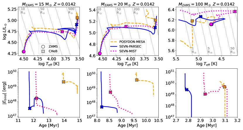
Figure 24: Comparison among posydon using mesa tracks (Fragos et al. 2023, orange dashed lines), sevn using parsec tracks (with overshooting parameter $\lambda_{\mathrm{ov}}=0.5$, blue solid lines), and sevn using mist tracks (Choi et al. 2016, magenta dotted lines) for stars with $M_{\rm ZAMS}=15$, 20, 100 M_⊙ (from left to right), and metallicity $Z=0.0142$. Upper panels: HR diagrams. The grey dashed lines indicate points at constant radius: 1, 2, 5, 10, 20, 50, 100, 200, 500, 1000, and 2000 R_⊙. Lower panels: evolution of the envelope binding energy estimated following the Claeys et al. (2014) formalism for sevn.(Appendix A.1.4) and taken directly from the tracks for posydon. The envelope binding energy is shown only when the mass of the helium core is larger than 0.1 M_⊙. The markers indicate the starting position in the ZAMS (circles), and the core He burning (CHeB) ignition estimated as described in Appendix B (crosses).

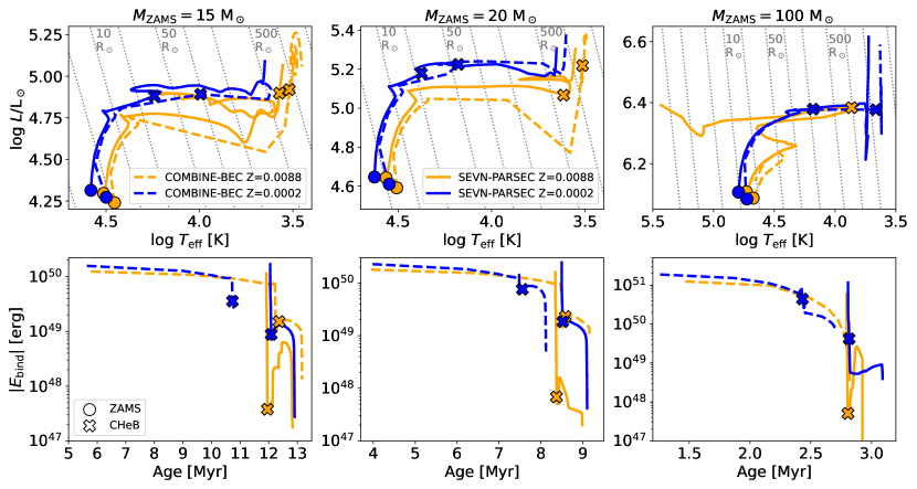
Figure 25: Same as Fig. 24, but comparing stars with metallicity Z=0.0088 (orange), Z=0.0002 (blue) computed by sevn using parsec stellar tables with overshooting parameter $\lambda_{\mathrm{ov}}=0.5$ (solid lines) , and by combine using bec tracks (Kruckow et al. 2018, dashed lines).

Figures 24 and 25 compare the evolution of stars integrated with sevn using the parsec tables ($\lambda_{\mathrm{ov}}=0.5$, Section 3.1) with sevn using the mist tracks (Choi et al., 2016), with posydon using mesa tracks (Fragos et al., 2023), and with combine (Kruckow et al., 2018) using bec (Yoon et al., 2010; Szécsi et al., 2015) tracks (Kruckow, private communication). We consider stars with $M_{\mathrm{ZAMS}}=15,20,100\ \ \mbox{M${}_{\odot}$}$ corresponding to NS progenitors, to the NS/BH formation boundary, and to high-mass BH progenitors, respectively. We use the metallicity $Z=0.0142$ (the metallicity currently available in posydon) for the comparison with parsec+mist and posydon, while $Z=0.0088$ and $Z=0.0002$ for the comparison with combine corresponding to their MW-like and IZw18-like models (Brott et al., 2011; Szécsi et al., 2015).

The stars in sevn+parsec, posydon and combine show a similar evolution in the HR diagram. In particular, intermediate-mass stars ($M_{\mathrm{ZAMS}}\lesssim 20\ \mbox{M${}_{\odot}$}$) at high-metallicity ignite the core He burning in the red part of the HR diagram ($T_{\mathrm{eff}}<4000\ \mathrm{K}$), while in the high-mass high-metallicity range the stars move to the blue before the ignition of the core He burning.

In contrast, stars evolved with sevn+mist show many similarities with the stellar evolution of bse-like codes: intermediate-mass stars begin core He burning while they are still hot and relatively compact, and high-metallicity massive stars move to the blue only after the ignition of the core He burning.

Overall, stars in posydon and mist live $\approx 10\mathrm{-}20\%$ longer than stars in parsec, while the stellar lifetimes are similar between parsec and combine at $Z=0.0088$, but stars in combine have a shorter ($\approx 10\mathrm{-}20\%$) life at $Z=0.0002$. On average, stars in combine and mist reach larger radii with respect to parsec and posydon.

The envelope binding energy of the stars in posydon and combine is 1–2 orders of magnitude larger than the values estimated in sevn for parsec and mist using the Claeys et al. (2014) formalism (Appendix A.1.4). Such difference can have a substantial impact on the production of merging BCOs (see, e.g., Section 4.2.4 and Section 5.2). The large discrepancy in the starting ages between parsec and bec (lower panels of Fig. 25) depends on the different assumptions used to define the He core. In this work, we consider the He core mass larger than zero when the central mass fraction of hydrogen is less than 0.001 (Section 3.1). In the combine+bec tracks, the core-envelope boundary is located at the point in which the hydrogen mass fraction is 0.1, but then the position of the boundary is further refined based on the average chemical abundances (Kruckow, private communication). Different definitions of the core-envelope boundary have a strong impact in the estimate of the envelope binding energy (see e.g., Kruckow et al., 2016).

Appendix D Analytic approximations for the GW merger time

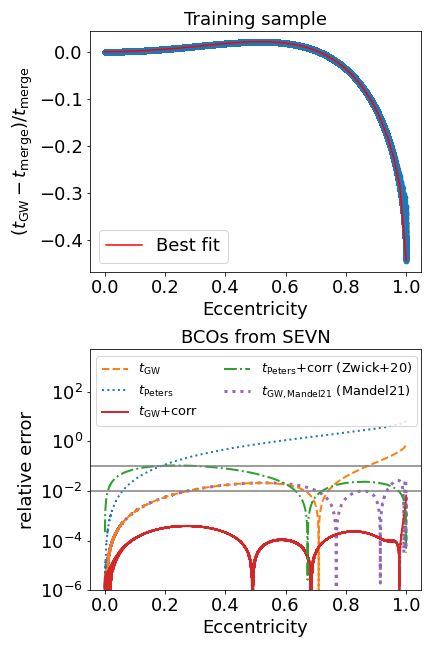
Figure 26: Upper panel: the blue thick line shows the relative difference between the GW-induced merging time estimated integrating Eqs. 39 and 40 and the analytic approximation $t_{\mathrm{GW}}$ in Eq. 70. The times have been estimated considering $5\times{}10^{5}$ BCOs with randomly drawn initial conditions, see text for further details. The red line is an analytic equation fitted to the blue points (Eq. 73). Lower panel: Same as the top panel but considering the absolute values of relative errors for a sample of $6\times{}10^{4}$ BCOs drawn from the fiducial simulations (see Sections 3.2 and 3.3) and different merging time approximations: $t_{\mathrm{peters}}$, blue dotted line, Eq. 69; $t_{\mathrm{GW}}$, orange dashed line, Eq. 70; $t_{\mathrm{peters+corr}}$ (Zwick et al., 2020), green dot-dashed line, Eq. 71; $t_{\mathrm{GW,Mandel21}}$ (Mandel, 2021), purple dotted line, Eq. 72; $t_{\mathrm{GW+corr}}$, red solid line, Eq. 74.

Method	Time per system averaged, C++ (s)	Time per system averaged, Python (s)	Average relative error	Maximum relative error
Adaptive 4th order Runge-Kutta	$1.1\times 10^{-3}$	$1.0\times 10^{-1}$	benchmark model	benchmark model
Adaptive Euler	$3.0\times 10^{-4}$	$2.8\times 10^{-3}$	$3.8\times 10^{-3}$	$2.7\times 10^{-2}$
$t_{\mathrm{peters}}$ (Eq. 69)	$2.9\times 10^{-8}$	$4.3\times 10^{-8}$	$4.9\times 10^{-1}$	$8.7\times 10^{-1}$
$t_{\mathrm{GW}}$ (Eq. 70)	$3.0\times 10^{-8}$	$3.4\times 10^{-8}$	$7.3\times 10^{-2}$	$4.3\times 10^{-1}$
$t_{\mathrm{peters+corr}}$ (Zwick et al. 2020, Eq. 71)	$4.5\times 10^{-8}$	$6.0\times 10^{-8}$	$4.5\times 10^{-2}$	$1.1\times 10^{-1}$
$t_{\mathrm{GW,Mandel21}}$ (Mandel 2021, Eq. 72)	$7.9\times 10^{-8}$	$8.6\times 10^{-8}$	$9.4\times 10^{-3}$	$2.8\times 10^{-2}$
$t_{\mathrm{GW+corr}}$ (Eq. 74)	$8.4\times 10^{-8}$	$9.7\times 10^{-8}$	$1.7\times 10^{-4}$	$5.6\times 10^{-3}$
$t_{\mathrm{merge}}$ (Eq. 75)	$8.4\times 10^{-8}$	$1.3\times 10^{-7}$	$1.7\times 10^{-4}$	$3.3\times 10^{-3}$

Table 8: Performance of different methods to estimate the GW-induced merger time. The first two methods use a 4th order Runge-Kutta (first row) or Euler (second row) solver with an an adaptive time-step scheme. All the other methods are analytic approximations (further details are given in the main text). The second and third columns contain the average computational time required to estimate the merging time of a single system in C++ and Python. The fourth and fifth columns contain the average and maximum relative differences of a given method with respect to the merging times estimated with the adaptive 4th order Runge-Kutta scheme. The values reported in this table have been obtained estimating the merger time for $6\times{}10^{4}$ BCOs sampled from our fiducial model (Section 3.2). We performed this computation using a serial code and a 3.1 GHz Quad-Core Intel Core i7 processor. The Python script exploits numpy vectorisation. We compiled the C++ code with the maximum allowed optimisation flag ($-\mathrm{O}3$). The C++ code used to perform this analysis can be found in the gitlab repository of the paper ().

The GW-induced merger time is estimated integrating Eqs. 39 and 40.

We test both performance of an adaptive time-step scheme applied to a 4th order Runge-Kutta and Euler solvers. We stop the integration when the semi-major axis becomes smaller than the innermost stable circular orbit (three times the Schwarzchild radius) of the most massive object. The Runge-Kutta solver offers the most precise evaluation of the merger time at the cost of relatively high computation time, especially using Python (0.1s per integration). In the rest of the Appendix, we consider the merger time estimated with the 4th order Runge-Kutta integration, $t_{\mathrm{RK}}$, our benchmark to evaluate the performance of other methods. The Euler solver offers a factor of $\approx{3}$ speedup at the cost of an average $\approx 0.4\%$ error and maximum error $\approx 3\%$.

We can obtain an approximation of merging time integrating Eq. 39 by assuming that the eccentricity remains constant during the evolution:

$$t_{\mathrm{peters}}=\frac{5}{256}\frac{c^{5}}{G^{3}}\frac{a^{4}}{M_{1}M_{2}(M_{1}+M_{2})}\frac{(1-e^{2})^{\frac{7}{2}}}{\left(1+\frac{73}{24}e^{2}+\frac{37}{96}e^{4}\right)}$$ (69)

Figure 26 shows that $t_{\mathrm{peters}}$ quickly diverges from $t_{\mathrm{RK}}$ for $e>0.1$, in particular, it tends to progressively underestimate the merger time with increasing eccentricity. To reduce the time difference, we remove the part of the denominator depending on the eccentricity in Eq. 69:

$$t_{\mathrm{GW}}=\frac{5}{256}\frac{c^{5}}{G^{3}}\frac{a^{4}}{M_{1}M_{2}(M_{1}+M_{2})}(1-e^{2})^{\frac{7}{2}}.$$ (70)

Figure 26 indicates that this simple modification is enough to have a good approximation of the merger time (within a few %) up to $e\approx 0.8$.

Zwick et al. (2020) found that the ratio between $t_{\mathrm{peters}}$ and the properly integrated merging time depends solely on the eccentricity (see also Peters 1964b), hence they introduced a correction term on $t_{\mathrm{peters}}$:

$$t_{\mathrm{peters+corr}}=t_{\mathrm{peters}}\,{}8^{1-\sqrt{1-e}}.$$ (71)

Eq. 71 represents a solid improvement with respect to $t_{\mathrm{peters}}$, especially for very large eccentricities (see Fig. 26). However, it gives a less precise approximation with respect to $t_{\mathrm{GW}}$ for low eccentricities ($e<0.5$).

Similarly, Mandel (2021) proposed an analytic approximation for the GW-induced merger time,

$$t_{\mathrm{GW,Mandel21}}=t_{\mathrm{GW}}(1+0.27e^{10}+0.33e^{20}+0.2e^{100}),$$ (72)

that is accurate to within 3% over the entire range of initial eccentricities (Fig. 26).

Based on Zwick et al. (2020) and Mandel (2021), we aim to find a correction term for $t_{\mathrm{GW}}$. We produce a training set randomly drawing the initial conditions of $5\times{}10^{5}$ BCOs. The masses are sampled uniformly between 0.5 and 300 $\mathrm{M}_{\odot}$, the semi-major axis is sampled uniformly in the logarithmic space between $10^{-1}$ and $10^{10}$ $\mathrm{R}_{\odot}$. Finally, for half of the sample the eccentricity is drawn uniformly between 0 and 0.95, for the other half between 0.95 and 1. The upper panel of Fig. 26 shows the relative difference between $t_{\mathrm{RK}}$ and $t_{\mathrm{GW}}$. We fit the relative error curve with an analytic equation deriving the correction term:

$$f_{\mathrm{corr}}=e^{2}\left[-0.443+0.580\left(1-e^{3.074}\right)^{1.105-0.807e+0.193e^{2}}\right].$$ (73)

Finally, the GW-induced merger time is approximated as

$$t_{\mathrm{GW+corr}}=\frac{t_{\mathrm{GW}}}{1+f_{\mathrm{corr}}(e)}.$$ (74)

Eq. 74 outperforms all the other tested approximations, and performs even better than the Euler solver (see Table 8). For most of the eccentricity range, the relative errors are less than 0.02% (see Fig. 26). Only for very extreme eccentricities ($e>0.99$), $t_{\mathrm{GW+corr}}$ begins to produce progressively larger errors, but still contained within $0.6\%$ (maximum relative error at $e=0.99999$).

The reason for this decrease in precision is evident in the upper panel of Fig. 26. Around $e=0.99$, the relative residuals show an abrupt drop that cannot be properly modelled by the fitting equation.

Figure 26 shows that the relative error curves of the $t_{\mathrm{GW+peters}}$ (Eq. 71) and $t_{\mathrm{GW+corr}}$ (Eq. 74) cross at $e\approx 0.999$. We can exploit the best of the two approximations defining:

$$t_{\mathrm{merge}}=\begin{cases}t_{\mathrm{GW+corr}}\ \ \mathrm{for}\ e<0.999\\ t_{\mathrm{peters+corr}}\ \ \mathrm{for}\ e\geq 0.999\end{cases}$$ (75)

Eq. 75 offers a high-precision approximation of the merger time on the whole eccentricity range at the expense of a negligible computation overhead. Obviously, all the analytic approximations outperform the adaptive integration in terms of computational time. The speedup is a factor of $10^{4}\mathrm{-}10^{5}$ in C++ and $10^{5}\mathrm{-}10^{7}$ in Python (Table 8).

Zwick et al. (2020) and Zwick et al. (2021) introduced additional correction factors to account for post-Newtonian terms (see also Will & Maitra, 2017; Tucker & Will, 2021). We checked that the corrections are negligible for all the BCOs systems tested in our analysis ($5\times{}10^{5}$ systems with randomly drawn initial conditions and $6\times{}10^{4}$ systems from the fiducial model, see Sections 3.2 and 3.3). Only systems with an initial tight configuration are significantly affected. Such systems merge in a very short time (close to the first periastron passage). Therefore, even if the relative errors could be large, the absolute time difference is negligible for any practical purpose concerning population synthesis studies.

All the methods discussed in this Appendix are implemented in the function estimate_tgw contained in the publicly available Python module pyblack.

References

- Abbott et al. (2016a) Abbott B. P., et al., 2016a, Physical Review X, 6, 041015
- Abbott et al. (2016b) Abbott B. P., et al., 2016b, Phys. Rev. Lett., 116, 061102
- Abbott et al. (2016c) Abbott B. P., et al., 2016c, ApJ, 818, L22
- Abbott et al. (2017a) Abbott B. P., et al., 2017a, Physical Review Letters, 119, 161101
- Abbott et al. (2017b) Abbott B. P., et al., 2017b, ApJ, 848, L12
- Abbott et al. (2019a) Abbott B. P., et al., 2019a, Physical Review X, 9, 031040
- Abbott et al. (2019b) Abbott B. P., et al., 2019b, ApJ, 882, L24
- Abbott et al. (2020a) Abbott R., et al., 2020a, Phys. Rev. Lett., 125, 101102
- Abbott et al. (2020b) Abbott B. P., et al., 2020b, ApJ, 892, L3
- Abbott et al. (2020c) Abbott R., et al., 2020c, ApJ, 896, L44
- Abbott et al. (2020d) Abbott R., et al., 2020d, ApJ, 900, L13
- Abbott et al. (2021a) Abbott R., et al., 2021a, arXiv e-prints, p. arXiv:2108.01045
- Abbott et al. (2021b) Abbott R., et al., 2021b, arXiv e-prints, p. arXiv:2111.03606
- Abbott et al. (2021c) Abbott R., et al., 2021c, Physical Review X, 11, 021053
- Abbott et al. (2021d) Abbott R., et al., 2021d, ApJ, 913, L7
- Abbott et al. (2023) Abbott R., et al., 2023, Physical Review X, 13, 011048
- Aghanim et al. (2020) Aghanim N., et al., 2020, A&A, 641, A6
- Agrawal et al. (2020) Agrawal P., Hurley J., Stevenson S., Szécsi D., Flynn C., 2020, MNRAS, 497, 4549
- Ali-Haïmoud et al. (2017) Ali-Haïmoud Y., Kovetz E. D., Kamionkowski M., 2017, Phys. Rev. D, 96, 123523
- Arca Sedda (2020) Arca Sedda M., 2020, ApJ, 891, 47
- Arca Sedda et al. (2020) Arca Sedda M., Mapelli M., Spera M., Benacquista M., Giacobbo N., 2020, ApJ, 894, 133
- Arca Sedda et al. (2021a) Arca Sedda M., Li G., Kocsis B., 2021a, A&A, 650, A189
- Arca-Sedda et al. (2021b) Arca-Sedda M., Rizzuto F. P., Naab T., Ostriker J., Giersz M., Spurzem R., 2021b, ApJ, 920, 128
- Atri et al. (2019) Atri P., et al., 2019, MNRAS, 489, 3116
- Banerjee (2017) Banerjee S., 2017, MNRAS, 467, 524
- Banerjee (2018) Banerjee S., 2018, MNRAS, 473, 909
- Banerjee (2021) Banerjee S., 2021, MNRAS, 500, 3002
- Banerjee et al. (2010) Banerjee S., Baumgardt H., Kroupa P., 2010, MNRAS, 402, 371
- Banerjee et al. (2020) Banerjee S., Belczynski K., Fryer C. L., Berczik P., Hurley J. R., Spurzem R., Wang L., 2020, A&A, 639, A41
- Barkat et al. (1967) Barkat Z., Rakavy G., Sack N., 1967, Phys. Rev. Lett., 18, 379
- Belczynski et al. (2002) Belczynski K., Kalogera V., Bulik T., 2002, ApJ, 572, 407
- Belczynski et al. (2008) Belczynski K., Kalogera V., Rasio F. A., Taam R. E., Zezas A., Bulik T., Maccarone T. J., Ivanova N., 2008, ApJS, 174, 223
- Belczynski et al. (2018) Belczynski K., et al., 2018, A&A, 615, A91
- Bethe & Brown (1998) Bethe H. A., Brown G. E., 1998, ApJ, 506, 780
- Bird et al. (2016) Bird S., Cholis I., Muñoz J. B., Ali-Haïmoud Y., Kamionkowski M., Kovetz E. D., Raccanelli A., Riess A. G., 2016, Physical Review Letters, 116, 201301
- Blaauw (1961) Blaauw A., 1961, Bull. Astron. Inst. Netherlands, 15, 265
- Boco et al. (2019) Boco L., Lapi A., Goswami S., Perrotta F., Baccigalupi C., Danese L., 2019, ApJ, 881, 157
- Böhm-Vitense (1958) Böhm-Vitense E., 1958, Z. Astrophys., 46, 108
- Bond et al. (1984) Bond J. R., Arnett W. D., Carr B. J., 1984, ApJ, 280, 825
- Bondi & Hoyle (1944) Bondi H., Hoyle F., 1944, MNRAS, 104, 273
- Bouffanais et al. (2021a) Bouffanais Y., Mapelli M., Santoliquido F., Giacobbo N., Iorio G., Costa G., 2021a, MNRAS, 505, 3873
- Bouffanais et al. (2021b) Bouffanais Y., Mapelli M., Santoliquido F., Giacobbo N., Iorio G., Costa G., 2021b, MNRAS, 505, 3873
- Breivik et al. (2020) Breivik K., et al., 2020, ApJ, 898, 71
- Bressan et al. (1981) Bressan A. G., Chiosi C., Bertelli G., 1981, A&A, 102, 25
- Bressan et al. (2012) Bressan A., Marigo P., Girardi L., Salasnich B., Dal Cero C., Rubele S., Nanni A., 2012, MNRAS, 427, 127
- Briel et al. (2023) Briel M. M., Stevance H. F., Eldridge J. J., 2023, MNRAS, 520, 5724
- Broekgaarden et al. (2021) Broekgaarden F. S., et al., 2021, MNRAS, 508, 5028
- Broekgaarden et al. (2022) Broekgaarden F. S., et al., 2022, MNRAS, 516, 5737
- Brott et al. (2011) Brott I., et al., 2011, A&A, 530, A116
- Brown (1995) Brown G. E., 1995, ApJ, 440, 270
- Caffau et al. (2011) Caffau E., Ludwig H. G., Steffen M., Freytag B., Bonifacio P., 2011, Sol. Phys., 268, 255
- Callister & Farr (2023) Callister T. A., Farr W. M., 2023, arXiv e-prints, p. arXiv:2302.07289
- Camacho et al. (2014) Camacho J., Torres S., García-Berro E., Zorotovic M., Schreiber M. R., Rebassa-Mansergas A., Nebot Gómez-Morán A., Gänsicke B. T., 2014, A&A, 566, A86
- Cantiello et al. (2007) Cantiello M., Yoon S. C., Langer N., Livio M., 2007, A&A, 465, L29
- Capano et al. (2020) Capano C. D., et al., 2020, Nature Astronomy, 4, 625
- Carr & Hawking (1974) Carr B. J., Hawking S. W., 1974, MNRAS, 168, 399
- Carr et al. (2016) Carr B., Kühnel F., Sandstad M., 2016, Phys. Rev. D, 94, 083504
- Chen et al. (2015) Chen Y., Bressan A., Girardi L., Marigo P., Kong X., Lanza A., 2015, MNRAS, 452, 1068
- Chieffi & Limongi (2013) Chieffi A., Limongi M., 2013, ApJ, 764, 21
- Choi et al. (2016) Choi J., Dotter A., Conroy C., Cantiello M., Paxton B., Johnson B. D., 2016, ApJ, 823, 102
- Chruslinska et al. (2019) Chruslinska M., Nelemans G., Belczynski K., 2019, MNRAS, 482, 5012
- Claeys et al. (2014) Claeys J. S. W., Pols O. R., Izzard R. G., Vink J., Verbunt F. W. M., 2014, A&A, 563, A83
- Claret & Torres (2018) Claret A., Torres G., 2018, ApJ, 859, 100
- Costa et al. (2019) Costa G., Girardi L., Bressan A., Marigo P., Rodrigues T. S., Chen Y., Lanza A., Goudfrooij P., 2019, MNRAS, 485, 4641
- Costa et al. (2021) Costa G., Bressan A., Mapelli M., Marigo P., Iorio G., Spera M., 2021, MNRAS, 501, 4514
- Costa et al. (2022) Costa G., Ballone A., Mapelli M., Bressan A., 2022, MNRAS, 516, 1072
- Costa et al. (2023) Costa G., Mapelli M., Iorio G., Santoliquido F., Escobar G. J., Klessen R. S., Bressan A., 2023, arXiv e-prints, p. arXiv:2303.15511
- Cyburt et al. (2010) Cyburt R. H., et al., 2010, ApJS, 189, 240
- De Donder & Vanbeveren (2004) De Donder E., Vanbeveren D., 2004, New Astron. Rev., 48, 861
- De Luca et al. (2021a) De Luca V., Desjacques V., Franciolini G., Pani P., Riotto A., 2021a, Phys. Rev. Lett., 126, 051101
- De Luca et al. (2021b) De Luca V., Franciolini G., Pani P., Riotto A., 2021b, J. Cosmology Astropart. Phys., 2021, 003
- De Marco et al. (2011) De Marco O., Passy J.-C., Moe M., Herwig F., Mac Low M.-M., Paxton B., 2011, Monthly Notices of the Royal Astronomical Society, 411, 2277
- Deloye & Taam (2010) Deloye C. J., Taam R. E., 2010, ApJ, 719, L28
- Dewi et al. (2006) Dewi J. D. M., Podsiadlowski P., Sena A., 2006, MNRAS, 368, 1742
- Di Carlo et al. (2019) Di Carlo U. N., Giacobbo N., Mapelli M., Pasquato M., Spera M., Wang L., Haardt F., 2019, MNRAS, 487, 2947
- Di Carlo et al. (2020a) Di Carlo U. N., Mapelli M., Bouffanais Y., Giacobbo N., Santoliquido F., Bressan A., Spera M., Haardt F., 2020a, MNRAS, 497, 1043
- Di Carlo et al. (2020b) Di Carlo U. N., et al., 2020b, MNRAS, 498, 495
- Di Carlo et al. (2021) Di Carlo U. N., et al., 2021, MNRAS, 507, 5132
- Di Stefano et al. (2023) Di Stefano R., Kruckow M. U., Gao Y., Neunteufel P. G., Kobayashi C., 2023, ApJ, 944, 87
- Dominik et al. (2012) Dominik M., Belczynski K., Fryer C., Holz D. E., Berti E., Bulik T., Mandel I., O’Shaughnessy R., 2012, ApJ, 759, 52
- Eggleton (1971) Eggleton P. P., 1971, MNRAS, 151, 351
- Eggleton (1983) Eggleton P. P., 1983, ApJ, 268, 368
- Eldridge & Stanway (2012) Eldridge J. J., Stanway E. R., 2012, MNRAS, 419, 479
- Eldridge & Stanway (2016) Eldridge J. J., Stanway E. R., 2016, MNRAS, 462, 3302
- Eldridge & Tout (2004) Eldridge J. J., Tout C. A., 2004, MNRAS, 353, 87
- Eldridge et al. (2008) Eldridge J. J., Izzard R. G., Tout C. A., 2008, MNRAS, 384, 1109
- Eldridge et al. (2011) Eldridge J. J., Langer N., Tout C. A., 2011, MNRAS, 414, 3501
- Eldridge et al. (2017) Eldridge J. J., Stanway E. R., Xiao L., McClelland L. A. S., Taylor G., Ng M., Greis S. M. L., Bray J. C., 2017, Publ. Astron. Soc. Australia, 34, e058
- Farah et al. (2023) Farah A. M., Edelman B., Zevin M., Fishbach M., María Ezquiaga J., Farr B., Holz D. E., 2023, arXiv e-prints, p. arXiv:2301.00834
- Farmer et al. (2019) Farmer R., Renzo M., de Mink S. E., Marchant P., Justham S., 2019, ApJ, 887, 53
- Farmer et al. (2020) Farmer R., Renzo M., de Mink S. E., Fishbach M., Justham S., 2020, ApJ, 902, L36
- Farr et al. (2011) Farr W. M., Sravan N., Cantrell A., Kreidberg L., Bailyn C. D., Mandel I., Kalogera V., 2011, ApJ, 741, 103
- Fernández et al. (2018) Fernández R., Quataert E., Kashiyama K., Coughlin E. R., 2018, MNRAS, 476, 2366
- Fields et al. (2018) Fields C. E., Timmes F. X., Farmer R., Petermann I., Wolf W. M., Couch S. M., 2018, ApJS, 234, 19
- Fragione & Loeb (2019) Fragione G., Loeb A., 2019, MNRAS, 486, 4443
- Fragione & Silk (2020) Fragione G., Silk J., 2020, MNRAS, 498, 4591
- Fragione et al. (2020) Fragione G., Loeb A., Rasio F. A., 2020, ApJ, 902, L26
- Fragos (2022) Fragos T., 2022, POSYDON data, doi:10.5281/zenodo.6655751, https://doi.org/10.5281/zenodo.6655751
- Fragos et al. (2019) Fragos T., Andrews J. J., Ramirez-Ruiz E., Meynet G., Kalogera V., Taam R. E., Zezas A., 2019, ApJ, 883, L45
- Fragos et al. (2023) Fragos T., et al., 2023, ApJS, 264, 45
- Franciolini et al. (2022) Franciolini G., et al., 2022, Phys. Rev. D, 105, 083526
- Fryer et al. (2012) Fryer C. L., Belczynski K., Wiktorowicz G., Dominik M., Kalogera V., Holz D. E., 2012, ApJ, 749, 91
- Gallegos-Garcia et al. (2021) Gallegos-Garcia M., Berry C. P. L., Marchant P., Kalogera V., 2021, ApJ, 922, 110
- Ge et al. (2010a) Ge H., Webbink R. F., Han Z., Chen X., 2010a, Ap&SS, 329, 243
- Ge et al. (2010b) Ge H., Hjellming M. S., Webbink R. F., Chen X., Han Z., 2010b, ApJ, 717, 724
- Ge et al. (2015) Ge H., Webbink R. F., Chen X., Han Z., 2015, ApJ, 812, 40
- Ge et al. (2020a) Ge H., Webbink R. F., Han Z., 2020a, ApJS, 249, 9
- Ge et al. (2020b) Ge H., Webbink R. F., Chen X., Han Z., 2020b, ApJ, 899, 132
- Ge et al. (2022) Ge H., et al., 2022, ApJ, 933, 137
- Georgy et al. (2013) Georgy C., Ekström S., Granada A., Meynet G., Mowlavi N., Eggenberger P., Maeder A., 2013, A&A, 553, A24
- Giacobbo & Mapelli (2018) Giacobbo N., Mapelli M., 2018, MNRAS, 480, 2011
- Giacobbo & Mapelli (2019) Giacobbo N., Mapelli M., 2019, MNRAS, 482, 2234
- Giacobbo & Mapelli (2020) Giacobbo N., Mapelli M., 2020, ApJ, 891, 141
- Giacobbo et al. (2018) Giacobbo N., Mapelli M., Spera M., 2018, MNRAS, 474, 2959
- Giersz et al. (2015) Giersz M., Leigh N., Hypki A., Lützgendorf N., Askar A., 2015, MNRAS, 454, 3150
- Gräfener & Hamann (2008) Gräfener G., Hamann W.-R., 2008, A&A, 482, 945
- Halabi et al. (2018) Halabi G. M., Izzard R. G., Tout C. A., 2018, MNRAS, 480, 5176
- Harris et al. (2020) Harris C. R., et al., 2020, Nature, 585, 357
- Heger et al. (2003) Heger A., Fryer C. L., Woosley S. E., Langer N., Hartmann D. H., 2003, ApJ, 591, 288
- Hirai & Mandel (2022) Hirai R., Mandel I., 2022, ApJ, 937, L42
- Hobbs et al. (2005) Hobbs G., Lorimer D. R., Lyne A. G., Kramer M., 2005, MNRAS, 360, 974
- Hunter (2007) Hunter J. D., 2007, Computing in Science & Engineering, 9, 90
- Hurley et al. (2000) Hurley J. R., Pols O. R., Tout C. A., 2000, MNRAS, 315, 543
- Hurley et al. (2002) Hurley J. R., Tout C. A., Pols O. R., 2002, MNRAS, 329, 897
- Hut (1981) Hut P., 1981, A&A, 99, 126
- Iben & Livio (1993) Iben Icko J., Livio M., 1993, PASP, 105, 1373
- Iglesias & Rogers (1996) Iglesias C. A., Rogers F. J., 1996, ApJ, 464, 943
- Iorio et al. (2023) Iorio et al., 2023, Daset from the paper "Compact object mergers: exploring uncertainties from stellar and binary evolution with SEVN", doi:10.5281/zenodo.7794546, https://doi.org/10.5281/zenodo.7794546
- Itoh et al. (2008) Itoh N., Uchida S., Sakamoto Y., Kohyama Y., Nozawa S., 2008, ApJ, 677, 495
- Ivanova & Taam (2004) Ivanova N., Taam R. E., 2004, ApJ, 601, 1058
- Ivanova et al. (2013a) Ivanova N., et al., 2013a, A&ARv, 21, 59
- Ivanova et al. (2013b) Ivanova N., et al., 2013b, A&ARv, 21, 59
- Izzard et al. (2004) Izzard R. G., Tout C. A., Karakas A. I., Pols O. R., 2004, MNRAS, 350, 407
- Izzard et al. (2006) Izzard R. G., Dray L. M., Karakas A. I., Lugaro M., Tout C. A., 2006, A&A, 460, 565
- Izzard et al. (2009) Izzard R. G., Glebbeek E., Stancliffe R. J., Pols O. R., 2009, A&A, 508, 1359
- Izzard et al. (2018) Izzard R. G., Preece H., Jofre P., Halabi G. M., Masseron T., Tout C. A., 2018, MNRAS, 473, 2984
- Jiménez-Forteza et al. (2017) Jiménez-Forteza X., Keitel D., Husa S., Hannam M., Khan S., Pürrer M., 2017, Phys. Rev. D, 95, 064024
- Justesen & Albrecht (2021) Justesen A. B., Albrecht S., 2021, ApJ, 912, 123
- Justham et al. (2011) Justham S., Podsiadlowski P., Han Z., 2011, MNRAS, 410, 984
- Kamlah et al. (2022) Kamlah A. W. H., et al., 2022, MNRAS, 511, 4060
- Kitaura et al. (2006) Kitaura F. S., Janka H. T., Hillebrandt W., 2006, A&A, 450, 345
- Kiziltan et al. (2013) Kiziltan B., Kottas A., De Yoreo M., Thorsett S. E., 2013, ApJ, 778, 66
- Klencki et al. (2020) Klencki J., Nelemans G., Istrate A. G., Pols O., 2020, A&A, 638, A55
- Klencki et al. (2021) Klencki J., Nelemans G., Istrate A. G., Chruslinska M., 2021, A&A, 645, A54
- Klencki et al. (2022) Klencki J., Istrate A., Nelemans G., Pols O., 2022, A&A, 662, A56
- Korol et al. (2022) Korol V., Belokurov V., Toonen S., 2022, MNRAS, 515, 1228
- Kremer et al. (2020a) Kremer K., et al., 2020a, ApJS, 247, 48
- Kremer et al. (2020b) Kremer K., et al., 2020b, ApJ, 903, 45
- Kroupa (2001) Kroupa P., 2001, MNRAS, 322, 231
- Kruckow et al. (2016) Kruckow M. U., Tauris T. M., Langer N., Szécsi D., Marchant P., Podsiadlowski P., 2016, A&A, 596, A58
- Kruckow et al. (2018) Kruckow M. U., Tauris T. M., Langer N., Kramer M., Izzard R. G., 2018, MNRAS, 481, 1908
- Kučinskas (1998) Kučinskas A., 1998, Ap&SS, 262, 127
- Lattimer & Yahil (1989) Lattimer J. M., Yahil A., 1989, ApJ, 340, 426
- Lau et al. (2022) Lau M. Y. M., Hirai R., González-Bolívar M., Price D. J., De Marco O., Mandel I., 2022, MNRAS, 512, 5462
- Law-Smith et al. (2020) Law-Smith J. A. P., et al., 2020, arXiv e-prints, p. arXiv:2011.06630
- Limongi & Chieffi (2018) Limongi M., Chieffi A., 2018, ApJS, 237, 13
- Lipunov et al. (1996) Lipunov V. M., Postnov K. A., Prokhorov M. E., 1996, A&A, 310, 489
- Lipunov et al. (2009) Lipunov V. M., Postnov K. A., Prokhorov M. E., Bogomazov A. I., 2009, Astronomy Reports, 53, 915
- Livio & Soker (1988) Livio M., Soker N., 1988, ApJ, 329, 764
- Lubow & Shu (1975) Lubow S. H., Shu F. H., 1975, ApJ, 198, 383
- Madau & Dickinson (2014) Madau P., Dickinson M., 2014, ARA&A, 52, 415
- Madau & Fragos (2017) Madau P., Fragos T., 2017, ApJ, 840, 39
- Mandel (2021) Mandel I., 2021, Research Notes of the American Astronomical Society, 5, 223
- Mandel & Farmer (2022) Mandel I., Farmer A., 2022, Phys. Rep., 955, 1
- Mandel & Fragos (2020) Mandel I., Fragos T., 2020, ApJ, 895, L28
- Mapelli (2016) Mapelli M., 2016, MNRAS, 459, 3432
- Mapelli (2021) Mapelli M., 2021, Formation Channels of Single and Binary Stellar-Mass Black Holes. Springer Singapore, Singapore, pp 1–65, doi:10.1007/978-981-15-4702-7_16-1, https://doi.org/10.1007/978-981-15-4702-7_16-1
- Mapelli et al. (2013) Mapelli M., Zampieri L., Ripamonti E., Bressan A., 2013, MNRAS, 429, 2298
- Mapelli et al. (2017) Mapelli M., Giacobbo N., Ripamonti E., Spera M., 2017, MNRAS, 472, 2422
- Mapelli et al. (2020) Mapelli M., Spera M., Montanari E., Limongi M., Chieffi A., Giacobbo N., Bressan A., Bouffanais Y., 2020, ApJ, 888, 76
- Mapelli et al. (2021) Mapelli M., et al., 2021, MNRAS, 505, 339
- Mapelli et al. (2022) Mapelli M., Bouffanais Y., Santoliquido F., Arca Sedda M., Artale M. C., 2022, MNRAS, 511, 5797
- Marchant & Moriya (2020) Marchant P., Moriya T. J., 2020, A&A, 640, L18
- Marchant et al. (2021) Marchant P., Pappas K. M. W., Gallegos-Garcia M., Berry C. P. L., Taam R. E., Kalogera V., Podsiadlowski P., 2021, A&A, 650, A107
- Marcussen & Albrecht (2022) Marcussen M. L., Albrecht S. H., 2022, ApJ, 933, 227
- Marigo & Aringer (2009) Marigo P., Aringer B., 2009, A&A, 508, 1539
- Mehta et al. (2022) Mehta A. K., Buonanno A., Gair J., Miller M. C., Farag E., deBoer R. J., Wiescher M., Timmes F. X., 2022, ApJ, 924, 39
- Meibom & Mathieu (2005) Meibom S., Mathieu R. D., 2005, ApJ, 620, 970
- Mennekens & Vanbeveren (2014) Mennekens N., Vanbeveren D., 2014, A&A, 564, A134
- Miller & Hamilton (2002) Miller M. C., Hamilton D. P., 2002, MNRAS, 330, 232
- Neijssel et al. (2019a) Neijssel C. J., et al., 2019a, MNRAS, 490, 3740
- Neijssel et al. (2019b) Neijssel C. J., et al., 2019b, MNRAS, 490, 3740
- Ng et al. (2022) Ng K. K. Y., Franciolini G., Berti E., Pani P., Riotto A., Vitale S., 2022, ApJ, 933, L41
- Nguyen et al. (2022) Nguyen C. T., et al., 2022, A&A, 665, A126
- Nugis & Lamers (2000) Nugis T., Lamers H. J. G. L. M., 2000, A&A, 360, 227
- O’Connor & Ott (2011) O’Connor E., Ott C. D., 2011, ApJ, 730, 70
- Ober et al. (1983) Ober W. W., El Eid M. F., Fricke K. J., 1983, A&A, 119, 61
- Özel & Freire (2016) Özel F., Freire P., 2016, ARA&A, 54, 401
- Özel et al. (2010) Özel F., Psaltis D., Narayan R., McClintock J. E., 2010, ApJ, 725, 1918
- Özel et al. (2012) Özel F., Psaltis D., Narayan R., Santos Villarreal A., 2012, ApJ, 757, 55
- Patton & Sukhbold (2020) Patton R. A., Sukhbold T., 2020, MNRAS, 499, 2803
- Pavlovskii et al. (2017) Pavlovskii K., Ivanova N., Belczynski K., Van K. X., 2017, MNRAS, 465, 2092
- Paxton et al. (2011) Paxton B., Bildsten L., Dotter A., Herwig F., Lesaffre P., Timmes F., 2011, ApJS, 192, 3
- Paxton et al. (2013) Paxton B., et al., 2013, ApJS, 208, 4
- Paxton et al. (2015) Paxton B., et al., 2015, ApJS, 220, 15
- Paxton et al. (2018) Paxton B., et al., 2018, ApJS, 234, 34
- Perez & Granger (2007) Perez F., Granger B. E., 2007, Computing in Science Engineering, 9, 21
- Peters (1964a) Peters P. C., 1964a, Physical Review, 136, 1224
- Peters (1964b) Peters P. C., 1964b, Phys. Rev., 136, B1224
- Petrovic et al. (2005) Petrovic J., Langer N., van der Hucht K. A., 2005, A&A, 435, 1013
- Pols et al. (1995) Pols O. R., Tout C. A., Eggleton P. P., Han Z., 1995, MNRAS, 274, 964
- Pols et al. (1998) Pols O. R., Schröder K.-P., Hurley J. R., Tout C. A., Eggleton P. P., 1998, MNRAS, 298, 525
- Portegies Zwart & Verbunt (1996) Portegies Zwart S. F., Verbunt F., 1996, A&A, 309, 179
- Poutanen (2017) Poutanen J., 2017, ApJ, 835, 119
- Ragoler et al. (2022) Ragoler N., Bear E., Schreier R., Hillel S., Soker N., 2022, MNRAS, 515, 5473
- Rappaport et al. (1983) Rappaport S., Verbunt F., Joss P. C., 1983, ApJ, 275, 713
- Rasio et al. (1996) Rasio F. A., Tout C. A., Lubow S. H., Livio M., 1996, ApJ, 470, 1187
- Rastello et al. (2019) Rastello S., Amaro-Seoane P., Arca-Sedda M., Capuzzo-Dolcetta R., Fragione G., Tosta e Melo I., 2019, MNRAS, 483, 1233
- Rastello et al. (2020) Rastello S., Mapelli M., Di Carlo U. N., Giacobbo N., Santoliquido F., Spera M., Ballone A., Iorio G., 2020, MNRAS, 497, 1563
- Rastello et al. (2021) Rastello S., Mapelli M., Di Carlo U. N., Iorio G., Ballone A., Giacobbo N., Santoliquido F., Torniamenti S., 2021, MNRAS, 507, 3612
- Renzo et al. (2020a) Renzo M., Farmer R. J., Justham S., de Mink S. E., Götberg Y., Marchant P., 2020a, MNRAS, 493, 4333
- Renzo et al. (2020b) Renzo M., Cantiello M., Metzger B. D., Jiang Y. F., 2020b, ApJ, 904, L13
- Riley et al. (2022) Riley J., et al., 2022, ApJS, 258, 34
- Rodriguez et al. (2015) Rodriguez C. L., Morscher M., Pattabiraman B., Chatterjee S., Haster C.-J., Rasio F. A., 2015, Physical Review Letters, 115, 051101
- Rodriguez et al. (2016) Rodriguez C. L., Chatterjee S., Rasio F. A., 2016, Phys. Rev. D, 93, 084029
- Röpke & De Marco (2023) Röpke F. K., De Marco O., 2023, Living Reviews in Computational Astrophysics, 9, 2
- Sallaska et al. (2013) Sallaska A. L., Iliadis C., Champange A. E., Goriely S., Starrfield S., Timmes F. X., 2013, ApJS, 207, 18
- Sana et al. (2012) Sana H., et al., 2012, Science, 337, 444
- Sander et al. (2019) Sander A. A. C., Hamann W. R., Todt H., Hainich R., Shenar T., Ramachandran V., Oskinova L. M., 2019, A&A, 621, A92
- Santoliquido et al. (2020) Santoliquido F., Mapelli M., Bouffanais Y., Giacobbo N., Di Carlo U. N., Rastello S., Artale M. C., Ballone A., 2020, ApJ, 898, 152
- Santoliquido et al. (2021) Santoliquido F., Mapelli M., Giacobbo N., Bouffanais Y., Artale M. C., 2021, MNRAS, 502, 4877
- Santoliquido et al. (2022) Santoliquido F., Mapelli M., Artale M. C., Boco L., 2022, MNRAS, 516, 3297
- Scelfo et al. (2018) Scelfo G., Bellomo N., Raccanelli A., Matarrese S., Verde L., 2018, J. Cosmology Astropart. Phys., 9, 039
- Schneider et al. (2015) Schneider F. R. N., Izzard R. G., Langer N., de Mink S. E., 2015, ApJ, 805, 20
- Schwarzschild (1958) Schwarzschild M., 1958, Structure and evolution of the stars.. Princeton, Princeton University Press, 1958.
- Shao & Li (2021) Shao Y., Li X.-D., 2021, ApJ, 920, 81
- Soberman et al. (1997) Soberman G. E., Phinney E. S., van den Heuvel E. P. J., 1997, A&A, 327, 620
- Spera & Mapelli (2017) Spera M., Mapelli M., 2017, MNRAS, 470, 4739
- Spera et al. (2015) Spera M., Mapelli M., Bressan A., 2015, MNRAS, 451, 4086
- Spera et al. (2019) Spera M., Mapelli M., Giacobbo N., Trani A. A., Bressan A., Costa G., 2019, MNRAS, 485, 889
- Szécsi et al. (2015) Szécsi D., Langer N., Yoon S.-C., Sanyal D., de Mink S., Evans C. J., Dermine T., 2015, A&A, 581, A15
- Tanikawa (2013) Tanikawa A., 2013, MNRAS, 435, 1358
- Tauris & van den Heuvel (2006) Tauris T. M., van den Heuvel E. P. J., 2006, in , Vol. 39, Compact stellar X-ray sources. Cambridge University Press, pp 623–665
- Tauris et al. (2015) Tauris T. M., Langer N., Podsiadlowski P., 2015, MNRAS, 451, 2123
- Tauris et al. (2017) Tauris T. M., et al., 2017, ApJ, 846, 170
- Temmink et al. (2023) Temmink K. D., Pols O. R., Justham S., Istrate A. G., Toonen S., 2023, A&A, 669, A45
- Timmes & Arnett (1999) Timmes F. X., Arnett D., 1999, ApJS, 125, 277
- Toonen & Nelemans (2013) Toonen S., Nelemans G., 2013, A&A, 557, A87
- Toonen et al. (2012) Toonen S., Nelemans G., Portegies Zwart S., 2012, A&A, 546, A70
- Torniamenti et al. (2022) Torniamenti S., Rastello S., Mapelli M., Di Carlo U. N., Ballone A., Pasquato M., 2022, MNRAS, 517, 2953
- Trani et al. (2022) Trani A. A., Rieder S., Tanikawa A., Iorio G., Martini R., Karelin G., Glanz H., Portegies Zwart S., 2022, Phys. Rev. D, 106, 043014
- Tucker & Will (2021) Tucker A., Will C. M., 2021, Phys. Rev. D, 104, 104023
- Tutukov & Yungelson (1996) Tutukov A., Yungelson L., 1996, MNRAS, 280, 1035
- Ulrich & Burger (1976) Ulrich R. K., Burger H. L., 1976, ApJ, 206, 509
- Vanbeveren et al. (1998) Vanbeveren D., De Donder E., Van Bever J., Van Rensbergen W., De Loore C., 1998, New Astron., 3, 443
- Vigna-Gómez et al. (2018) Vigna-Gómez A., et al., 2018, MNRAS, 481, 4009
- Vigna-Gómez et al. (2022) Vigna-Gómez A., Wassink M., Klencki J., Istrate A., Nelemans G., Mandel I., 2022, MNRAS, 511, 2326
- Vink et al. (2000) Vink J. S., de Koter A., Lamers H. J. G. L. M., 2000, A&A, 362, 295
- Vink et al. (2001) Vink J. S., de Koter A., Lamers H. J. G. L. M., 2001, A&A, 369, 574
- Vink et al. (2011) Vink J. S., Muijres L. E., Anthonisse B., de Koter A., Gräfener G., Langer N., 2011, A&A, 531, A132
- Vink et al. (2021) Vink J. S., Higgins E. R., Sander A. A. C., Sabhahit G. N., 2021, MNRAS, 504, 146
- Virtanen et al. (2020) Virtanen P., et al., 2020, Nature Methods, 17, 261
- Vos et al. (2015) Vos J., Østensen R. H., Marchant P., Van Winckel H., 2015, A&A, 579, A49
- Wang (2020) Wang L., 2020, MNRAS, 491, 2413
- Wang et al. (2022) Wang L., Tanikawa A., Fujii M., 2022, MNRAS, 515, 5106
- Webbink (1984) Webbink R. F., 1984, ApJ, 277, 355
- Webbink (1985) Webbink R. F., 1985, in Pringle J. E., Wade R. A., eds, , Interacting Binary Stars. Cambridge University Press, p. 39
- Webbink (1988) Webbink R. F., 1988, in Mikolajewska J., Friedjung M., Kenyon S. J., Viotti R., eds, Astrophysics and Space Science Library Vol. 145, IAU Colloq. 103: The Symbiotic Phenomenon. p. 311, doi:10.1007/978-94-009-2969-2_69
- Weiss et al. (2004) Weiss A., Hillebrandt W., Thomas H. C., Ritter H., 2004, Cox and Giuli’s Principles of Stellar Structure
- Will & Maitra (2017) Will C. M., Maitra M., 2017, Phys. Rev. D, 95, 064003
- Woosley (2017) Woosley S. E., 2017, ApJ, 836, 244
- Woosley (2019) Woosley S. E., 2019, ApJ, 878, 49
- Woosley et al. (2007) Woosley S. E., Blinnikov S., Heger A., 2007, Nature, 450, 390
- Woosley et al. (2020) Woosley S. E., Sukhbold T., Janka H. T., 2020, ApJ, 896, 56
- Wyrzykowski et al. (2016) Wyrzykowski Ł., et al., 2016, MNRAS, 458, 3012
- Xu & Li (2010a) Xu X.-J., Li X.-D., 2010a, ApJ, 716, 114
- Xu & Li (2010b) Xu X.-J., Li X.-D., 2010b, ApJ, 722, 1985
- Ye et al. (2022) Ye C. S., Kremer K., Rodriguez C. L., Rui N. Z., Weatherford N. C., Chatterjee S., Fragione G., Rasio F. A., 2022, ApJ, 931, 84
- Yoon et al. (2010) Yoon S. C., Woosley S. E., Langer N., 2010, ApJ, 725, 940
- Yoshida et al. (2016) Yoshida T., Umeda H., Maeda K., Ishii T., 2016, MNRAS, 457, 351
- Zahn (1975) Zahn J. P., 1975, A&A, 41, 329
- Zahn (1977) Zahn J. P., 1977, A&A, 57, 383
- Zevin et al. (2020) Zevin M., Spera M., Berry C. P. L., Kalogera V., 2020, ApJ, 899, L1
- Ziosi et al. (2014) Ziosi B. M., Mapelli M., Branchesi M., Tormen G., 2014, MNRAS, 441, 3703
- Zorotovic et al. (2010) Zorotovic M., Schreiber M. R., Gänsicke B. T., Nebot Gómez-Morán A., 2010, A&A, 520, A86
- Zwick et al. (2020) Zwick L., Capelo P. R., Bortolas E., Mayer L., Amaro-Seoane P., 2020, MNRAS, 495, 2321
- Zwick et al. (2021) Zwick L., Capelo P. R., Bortolas E., Vázquez-Aceves V., Mayer L., Amaro-Seoane P., 2021, MNRAS, 506, 1007
- de Mink et al. (2013) de Mink S. E., Langer N., Izzard R. G., Sana H., de Koter A., 2013, ApJ, 764, 166
- van Son et al. (2023) van Son L. A. C., de Mink S. E., Chruślińska M., Conroy C., Pakmor R., Hernquist L., 2023, ApJ, 948, 105
- van den Heuvel (1976) van den Heuvel E. P. J., 1976, in Eggleton P., Mitton S., Whelan J., eds, Astrophysics and Space Science Library Vol. 73, Structure and Evolution of Close Binary Systems. p. 35
- van den Heuvel (2007) van den Heuvel E. P. J., 2007, in di Salvo T., Israel G. L., Piersant L., Burderi L., Matt G., Tornambe A., Menna M. T., eds, American Institute of Physics Conference Series Vol. 924, The Multicolored Landscape of Compact Objects and Their Explosive Origins. pp 598–606 (arXiv:0704.1215), doi:10.1063/1.2774916
- van den Heuvel & De Loore (1973) van den Heuvel E. P. J., De Loore C., 1973, A&A, 25, 387
- van den Heuvel et al. (2017) van den Heuvel E. P. J., Portegies Zwart S. F., de Mink S. E., 2017, MNRAS, 471, 4256