Dark matter production via a non-minimal coupling to gravity

Oleg Lebedev^a, Timofey Solomko^b, Jong-Hyun Yoon^c

^aDepartment of Physics and Helsinki Institute of Physics,
Gustaf Hällströmin katu 2a, FI-00014 Helsinki, Finland
^bSaint Petersburg State University, 7/9 Universitetskaya nab.,
St.Petersburg, 199034, Russia
^cUniversité Paris-Saclay, CNRS/IN2P3, IJCLab, 91405 Orsay, France

Abstract

We study postinflationary scalar dark matter production via its non-minimal coupling to gravity. During the inflaton oscillation epoch, dark matter is produced resonantly for a sufficiently large non-minimal coupling $\xi\gtrsim 5$. We find that backreaction on the curvature and rescattering effects typically become important for the values of $\xi$ above $30$, which invalidate simple estimates of the production efficiency. At large couplings, the dark matter yield becomes almost independent of $\xi$, signifying approximate quasi-equilibrium in the inflaton-dark matter system. Although the analysis gets complicated by the presence of apparent negative energy in the Jordan frame, this behaviour can be regularized by introducing mild dark matter self-interaction. Using lattice simulations, we delineate parameter space leading to the correct dark matter relic abundance.

1 Introduction

Inflation is a cornerstone of modern cosmology, which explains many observed features of the Universe [1, 2, 3, 4, 5]. It also entails significant particle production of various kinds. In particular, inflationary and postinflationary particle production is an important source of stable relics, which may contribute to dark matter. It occurs due to non-adiabatic variation of the background field, e.g. the metric [6, 7] or the inflaton [8, 9] field. Recent reviews and discussions of the subject can be found in [10, 11].

In this work, we study postinflationary production of real scalar dark matter $s$ via its non-minimal coupling to curvature [12, 13],

$$\Delta\mathcal{L}_{\xi}=-{1\over 2}\xi R\,s^{2}\;,$$ (1)

where $\xi$ is a real constant. As $R$ starts oscillating after inflation, the effective mass term for $s$ changes its sign leading to efficient particle production. We assume that $s$ is stable and very weakly coupled such that it constitutes non-thermal dark matter (DM).

Particle production via a non-minimal coupling to gravity has been studied in a number of papers starting with [15]. Most work was focused on the linear regime, possibly including the Hartree approximation [16, 17, 18]. Dark matter with a non-minimal coupling to gravity was considered in [19, 20, 21, 22, 23] within the same approximation. Recently, this treatment has been improved in [25] by employing the quantum transport equations.

In our work, we make use of lattice simulations to incorporate important collective effects in dark matter production. We find that these crucially affect the resulting abundance, especially at large $\xi$. Such effects include significant backreaction of the produced particles on the curvature as well as rescattering, which lead to quasi-equilibrium in the inflaton-DM system at large $\xi$. In this regime, the dark matter abundance becomes almost independent of $\xi$. Analogous behaviour has been observed for direct inflaton-DM coupling in [26, 27].

We perform our computations in locally quadratic and quartic inflaton potentials, focussing on positive $\xi$ such that the field $s$ is sufficiently heavy during inflation and not subject to large de Sitter fluctuations. This allows us to use the vacuum state of the dark matter field as the initial condition for our simulations. In contrast, a negative $\xi$ leads to a large VEV of $s$ during inflation, which affects its eventual abundance. For comparison, however, we also display our results for $\xi<0$ with vacuum initial conditions, whenever possible. Finally, we delineate parameter space leading to the correct relic abundance of non-thermal dark matter.

2 Dynamics in the Jordan frame

In the Friedmann metric

$$ds^{2}=-dt^{2}+a(t)^{2}\,dx^{i}\,dx^{i}\;,$$ (2)

the scalar curvature is given by

$$R=6\left[{\ddot{a}\over a}+\left({\dot{a}\over a}\right)^{2}\right]\;,$$ (3)

where the dot indicates the time derivative. We take the action to be of the form

$$\mathcal{S}=\int d^{4}x\sqrt{-g}\left({1\over 2}M_{\textrm{Pl}}^{2}R-{1\over 2}\xi R\,s^{2}-{1\over 2}g^{\mu\nu}\partial_{\mu}s\,\partial_{\nu}s-{1\over 2}g^{\mu\nu}\partial_{\mu}\phi\,\partial_{\nu}\phi-V\right)\;,$$ (4)

where $s$ is the dark matter field, $\phi$ is the inflaton and $g$ is the metric determinant. We assume that the potential contains no direct coupling between $s$ and $\phi$, and can be approximated after inflation by

$$V=V(\phi)+V(s) ={1\over 2}m_{\phi}^{2}\phi^{2}+{1\over 4}\lambda_{\phi}\phi^{4}$$

$$+{1\over 2}m_{s}^{2}s^{2}+{1\over 4}\lambda_{s}s^{4}\;,$$ (5)

with $m_{\phi}\gg m_{s}$. We consider both possibilities that the inflaton potential during preheating is dominated by the quadratic or quartic parts.

In our study, we perform calculations in the Jordan frame following [28], that is, keeping explicit the coupling $s^{2}R$. This leads to simpler equations of motion compared to those in the Einstein frame. Indeed, the scalar kinetic terms in the Einstein frame are field-dependent and thus contain fast oscillating functions. This makes the numerical integration of the equations of motion relatively unstable compared to that in the Jordan frame. At late times, when the characteristic field value of $s$ becomes small, the Jordan and Einstein frames become essentially indistinguishable. As a result, the relevant observables such as (conserved) particle numbers can be read off directly from the simulation output in the Jordan frame. In practice, we terminate our simulation at $a/a_{0}\sim 10^{3}$ and compute the observables at that time.

An important aspect of the dynamics in the Jordan frame is the scalar mixing with the gravitational degrees of freedom [29]. In particular, the scale factor corresponds to a scalar component of the metric $g^{\mu\nu}$. Using (3) and integrating by parts, one finds the following kinetic terms:

$$\mathcal{K}={a^{3}\over 2}\,\dot{s}^{2}+6\xi a^{2}s\,\dot{a}\dot{s}+3a(\xi s^{2}-M_{\textrm{Pl}}^{2})\,\dot{a}^{2}\;.$$ (6)

We observe that there is kinetic mixing between $s$ and $a$, which can make a significant impact. For example, if we take $s$ to scale as radiation $s\sim a^{-1}$ at late times, the mixing term becomes much larger than the diagonal kinetic term $a^{3}\dot{s}^{2}$ at $\xi\gg 1$. On the other hand, the mixing is negligible if $s$ oscillates with a relatively large frequency $\omega\gg\xi H$ and decreasing amplitude $\propto a^{-\alpha}$ with $\alpha\sim\mathcal{O}(1)$. In this case, the scalar field decouples from the metric and one can define a meaningful oscillator number for its momentum modes.

The Einstein equation is obtained by varying the action with respect to $g^{\mu\nu}$,

$$R_{\mu\nu}-{1\over 2}g_{\mu\nu}R={1\over M_{\textrm{Pl}}^{2}}\,T_{\mu\nu}\;,$$ (7)

where the energy momentum tensor is

$$T_{\mu\nu}=-{2\over\sqrt{-g}}\,{\delta(\sqrt{-g}\mathcal{L}_{\textrm{matter}})\over\delta g^{\mu\nu}}\;.$$ (8)

The matter Lagrangian $\mathcal{L}_{\textrm{matter}}$ contains all the terms in the integrand of (4) except for ${1\over 2}M_{\textrm{Pl}}^{2}R$. In particular, the non–minimal gravity coupling to $s$ is considered part of $\mathcal{L}_{\textrm{matter}}$, in which case the energy momentum tensor is covariantly conserved by virtue of the Einstein equation. Furthermore, since there is no direct coupling between $\phi$ and $s$, the energy momentum tensor splits naturally into $T_{\mu\nu}(\phi)$ and $T_{\mu\nu}(s)$. An explicit calculation shows

$$T_{\mu\nu}(s)=\partial_{\mu}s\partial_{\nu}s-g_{\mu\nu}\left({1\over 2}g^{\rho\sigma}\partial_{\rho}s\,\partial_{\sigma}s+V(s)\right)+\xi\left(R_{\mu\nu}-{1\over 2}g_{\mu\nu}R+g_{\mu\nu}\Box-\nabla_{\mu}\nabla_{\nu}\right)s^{2}\;.$$ (9)

Here $\Box=g^{\mu\nu}\nabla_{\mu}\nabla_{\nu}$ and $\nabla_{\mu}$ is the covariant derivative associated with metric $g^{\mu\nu}$. A similar expression holds for $T_{\mu\nu}(\phi)$ except for the $\xi$–induced term.

The equation of motion for $s$ is obtained by varying the action with respect to $s$,

$$\Box s-\xi Rs-{\partial V\over\partial s}=0\;,$$ (10)

or

$$\ddot{s}+3{\dot{a}\over a}\,\dot{s}-{1\over a^{2}}\nabla^{2}s+\xi Rs+{\partial V\over\partial s}=0\;.$$ (11)

An analogous equation at $\xi=0$ applies to $\phi$. We note that the term $\xi R$ plays the role of the induced mass squared for dark matter. After inflation, the scalar curvature oscillates such that the effective mass of $s$ can turn tachyonic, indicating particle production.

Since gravity is represented by a single degree of freedom $a(t)$, it is sufficient to use the trace of the Einstein equation,

$$R=-{1\over M_{\textrm{Pl}}^{2}}T_{\mu}^{\mu}\;,$$ (12)

to solve for the evolution of the system. It simplifies further when one takes a spatial average of both sides of the equation. Since $T_{\mu\nu}$ itself depends on $R$, solving for $R$ yields

$$R={F(s)\over M_{\textrm{Pl}}^{2}}\left[(1-6\xi)\langle\partial^{\mu}s\partial_{\mu}s\rangle+4\langle V\rangle-6\xi\langle sV^{\prime}_{s}\rangle+\langle\partial^{\mu}\phi\,\partial_{\mu}\phi\rangle\right]\;,$$ (13)

where

$$F(s)\equiv\frac{1}{1+(6\xi-1)\xi\langle s^{2}\rangle/M_{\text{Pl}}^{2}}\,.$$ (14)

Expressing $R$ in terms of $a$ via (3), one obtains an equation of motion for $a(t)$, which, together with those for $s$ and $\phi$, can be solved numerically.

The initial evolution of $R$ is fully determined by the inflaton field. At later times, it can be significantly affected by the produced dark matter via the $\xi$-enhanced terms. In fact, such contributions are instrumental in determining the end of resonant particle production.

2.1 Negative energy and kinetic mixing

Having solved the EOM, one can determine the energy density of dark matter,

$$\rho(s)=\langle T_{00}(s)\rangle=\frac{1}{2}\langle\dot{s}^{2}\rangle+\frac{1}{2a^{2}}\langle(\nabla s)^{2}\rangle+\langle V(s)\rangle+3\xi H^{2}\langle s^{2}\rangle+6\xi H\langle s\dot{s}\rangle\;,$$ (15)

where we have dropped the term $\frac{\xi}{a^{2}}\langle\nabla^{2}s^{2}\rangle$, which averages to zero since $\nabla^{2}s^{2}$ is a total spatial derivative.

The interpretation of $\rho(s)$ is, however, not straightforward due to the presence of the last two terms. In particular, the term $6\xi H\langle s\dot{s}\rangle$ can be large and negative at large $\xi$ such that the total energy density becomes negative. For low frequency modes, this can persist even at asymptotically large times. Indeed, when the expansion is radiation–like, $R=0$, the late time low–$k$ solution to the EOM with $V(s)=0$ is $s\propto a^{-1}$. Then, using $\dot{s}=\dot{a}\,s^{\prime}_{a}$, one finds negative energy density for $\xi\gg 1$. The origin for this behaviour lies in the kinetic mixing between the scalar and the metric (6), which is responsible for the term $6\xi H\langle s\dot{s}\rangle$. The scalar energy density cannot in general be separated from that of gravity, however the scalar does ‘‘decouple’’ from the metric at late times when it has mass or self–interaction. This is because such terms decrease slower in time than the $\xi$-induced contributions do, thereby regularizing negative $\rho_{s}$. Since we are interested in small $m_{s}$, we make use of mild self–coupling $\lambda_{s}$, which allows us to define positive, conserved oscillator numbers at the end of the simulation.

In what follows, we study the system evolution and particle production in the $\phi^{4}$ and $\phi^{2}$ inflaton potentials.

3 Quartic local inflaton potential

Suppose that the bare inflaton mass $m_{\phi}$ is small compared to the relevant scales at the preheating epoch. Then, locally we can approximate the inflaton potential by the quartic term

$$V(\phi)\simeq{1\over 4}\lambda_{\phi}\,\phi^{4}\;.$$ (16)

Note that, at late times, when the characteristic momenta redshift to values comparable to $m_{\phi}$, the bare inflaton mass starts playing an important role.

In what follows, we study the main features of particle production in this system.

3.1 The resonance

Let us start with the case $\lambda_{s}=0$. The scalar curvature starts oscillating after inflation, leading to $s$-particle production (see Eq. (11)). This process can be described semi-classically in terms of the tachyonic resonance [30].

Initially, the energy density is dominated by the inflaton zero mode such that the curvature is given by

$$R=-{T_{\mu}^{\mu}(\phi)\over M_{\textrm{Pl}}^{2}}={1\over M_{\textrm{Pl}}^{2}}\left[4V(\phi)-\dot{\phi}^{2}\right]\;,$$ (17)

In the quartic potential, the inflaton field is given by [31]

$$\phi(t)=\phi_{0}\,\textrm{cn}\left(\sqrt{\lambda_{\phi}}\phi_{0}\,t,{1\over\sqrt{2}}\right)\;,$$ (18)

with a slowly varying amplitude

$$\phi_{0}\propto 1/a\;.$$ (19)

According to the convention of [31], cn$(x,1/\sqrt{2})$ satisfies $f^{\prime 2}(x)={1\over 2}\left[1-f^{4}(x)\right]$. Therefore,

$$R={\lambda_{\phi}\phi_{0}^{4}\over 2M_{\textrm{Pl}}^{2}}\,(3\,\textrm{cn}^{4}(\omega t)-1)\;,$$ (20)

where $\omega=\sqrt{\lambda_{\phi}}\phi_{0}$. In this expression, we keep only the leading term and neglect the derivatives of the scale factor.

Particle production is best analyzed in terms of the spacial Fourier modes of the DM field $s_{k}$ [31]. The equation of motion (Eq. (11)) for the rescaled $k$–modes $X_{k}=a^{3/2}s_{k}$ reads

$$\ddot{X}_{k}+\left({k^{2}\over a^{2}}+{9\over 4}wH^{2}+\xi R\right)\,X_{k}=0\;,$$ (21)

where $V(s)$ is assumed to be negligible and $w$ is the coefficient of the equation of state, $w=-(1+2\dot{H}/(3H^{2}))$. At large $\xi$, the $wH^{2}$ term can be omitted. Neglecting also the slow time variation of $\phi_{0}$, we get

$$X_{k}^{\prime\prime}+\left[\kappa+q\,\textrm{cn}^{4}(z)\right]\,X_{k}=0\;,$$ (22)

where

$$\kappa={k^{2}\over{\lambda_{\phi}}\phi_{0}^{2}a^{2}}-{\xi\phi_{0}^{2}\over 2M_{\textrm{Pl}}^{2}}~{}~{},~{}~{}q={3\xi\phi_{0}^{2}\over 2M_{\textrm{Pl}}^{2}}\;,$$ (23)

$z=\sqrt{\lambda_{\phi}}\phi_{0}\,t$ and the prime denotes differentiation with respect to $z$. As a result, we have broad tachyonic resonance: $q\gg 1$ and $\kappa<0$ for low momenta. Note that for a zero mode, $q/\kappa=-3$.

Figure 1: Stability charts for the ellipsoidal wave equation (22). Left: $\xi>0$; right: $\xi<0$. The color coding represents the Floquet exponent. The straight lines show an example of the time evolution of the coefficients for the zero and most excited $k_{\textrm{max}}$ modes at $\xi=30$.

The slow variation of $\phi_{0}$ and the oscillation frequency can readily be taken into account in conformal coordinates $\tau,Y_{k}$ defined by $dt=a\,d\tau$, $Y_{k}\equiv a\,s_{k}$. Instead of (21), one has

$$\ddot{Y_{k}}+\left({k^{2}}+\xi Ra^{2}-{\ddot{a}\over a}\right)\,Y_{k}=0\;,$$ (24)

where the dot now denotes differentiation with respect to $\tau$. In terms of the conformal time, $R=6\ddot{a}/a^{3}$, which shows that $\xi=1/6$ implies no particle production, as expected. At $\xi\gg 1$, the $\ddot{a}/a$ term can be neglected. The inflaton amplitude decreases according to $\phi_{0}=\Phi_{0}/a$, where $\Phi_{0}$ is the initial inflaton field value. Then, following [31], one can define $x\equiv\omega t={1\over 2}\sqrt{\lambda_{\phi}}\Phi_{0}\tau$ since $\tau\propto\sqrt{t}\propto a$. In terms of the time variable $x$, one then recovers Eq. (22) for $Y_{k}$ with $\kappa$ and $q$ rescaled by a factor of 4.

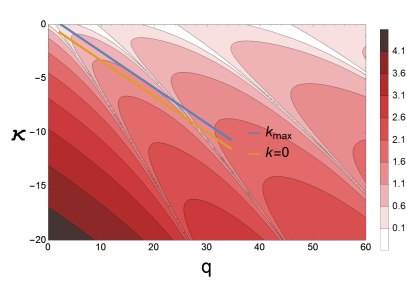
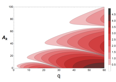
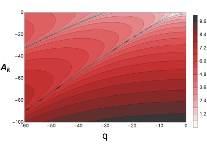
In the limit of constant coefficients, Eq. (22) belongs to the class of ellipsoidal or Lamé wave equations. The solution can oscillate or grow in time exponentially, depending on $\kappa$ and $q$. The corresponding stability charts are shown in Fig. 1. The color coding represents the value of the Floquet exponent $\mu$ such that the solution grows in time as $e^{\mu z}$ for a given set $\kappa,q$. This resonant amplification of the amplitude is interpreted as particle production.

For smaller momenta, particle production tends to be more efficient. However, the most excited momentum is not zero. The coefficients of the ellipsoidal wave equation are not exactly constant and evolve along straight lines in the $(q,\kappa)$ plane. As the system evolves, they pass through areas with different Floquet exponents and the mode that gets amplified the most over the course of this evolution dominates at the end of the simulation. For moderate $\xi$, we find

$$k_{\textrm{max}}^{2}\simeq 0.8\lambda_{\phi}\Phi_{0}^{2}\;.$$ (25)

The evolution of $\kappa,q$ for this and the zero modes is shown in Fig. 1.

At weak coupling, the most excited momentum mode of the inflaton field can be read off from the Lamé equation stability chart [31]. In the absence of other couplings, the system is conformal and the coefficients do not evolve in time, unlike in the above example. The inflaton self-interaction excites the mode with

$$k_{\textrm{max}}^{2}(\phi)\simeq 1.7\lambda_{\phi}\Phi_{0}^{2}\;.$$ (26)

The occupation number of the excited momentum modes peaks initially at this value, while subsequently the spectrum smoothens out due to rescattering.

We define the $k$-mode occupation numbers $n_{k}$ in the usual way. For example, in terms of the $Y_{k}$ variables and conformal time $\tau$, $n_{k}$ is given by

$$n_{k}\equiv\frac{1}{2}\left(\omega_{k}|Y_{k}|^{2}+\frac{1}{\omega_{k}}|\dot{Y}_{k}|^{2}\right)\;,$$ (27)

$$\omega^{2}_{k}\equiv k^{2}+a^{2}\left\langle\frac{\partial^{2}V(s)}{\partial s^{2}}\right\rangle\;.$$ (28)

As discussed above, this definition is meaningful in the Jordan frame only at late times, when $\rho(s)$ in (15) approaches the usual oscillator form. In this limit, one can also drop the $\xi R$ term from the EOM of $Y_{k}$. Integrating $n_{k}$ over $k$, one obtains the total particle number (see [26] for precise definitions).

The DM self-interaction is included in the above considerations using the Hartree approximation: it amounts to adding the mass-squared term proportional to $\lambda_{s}\langle s^{2}\rangle$ in the EOM for $s$. In the lattice formulation, however, this approximation is not necessary and the full interaction term ${1\over 4}\lambda_{s}s^{4}$, which mixes the different momentum modes, is accounted for.

3.2 End of resonance

In this subsection, we discuss the relevant time scales which determine the end of resonant dark matter production. This depends strongly on the couplings and there are several regimes. To understand the field dynamics in detail, we use classical lattice simulations. These are reliable if the occupation numbers are large enough, which corresponds to $\xi\gtrsim 5$ for positive $\xi$. We choose vacuum initial conditions for the field fluctuations. These are mimicked by the Rayleigh probability distribution for the momentum modes $|Y_{k}|$ [32],

$$P(Y_{k})\propto\exp(-2\omega_{k}|Y_{k}|^{2})\;,$$ (29)

where $\omega_{k}$ is the corresponding eigenfrequency at $t=0$. The phase of $Y_{k}$ is assumed to have a random uniform distribution. For the inflaton field, we take the initial conditions equivalent to

$$\Phi_{0}\simeq 0.9\,M_{\textrm{Pl}}$$ (30)

and zero initial velocity of $\phi$. In practice, it is more convenient to use a somewhat lower initial value of $\phi$ and a larger $\dot{\phi}$ corresponding to the same energy density. The simulations are performed with the numerical tool CosmoLattice [33, 34, 35] customized to account for the non-minimal coupling to gravity. Related particle production simulations in somewhat different regimes have been performed in [28, 36] and in [37, 38] with regard to the Higgs boson production.

In what follows, we define the end of the resonance as the period when the fast exponential growth of the occupation numbers terminates. We focus on $\xi>0$, although many statements apply, at least qualitatively, to the $\xi<0$ case as well modulo the replacement $\xi\to|\xi|$.

3.2.1 Moderate $\xi$ and $\lambda_{s}=0$

In the range $5\lesssim\xi\lesssim 30-40$, the resonance typically ends when the $q$–parameter ($\propto a^{-2}$) becomes sufficiently small,

$$q\lesssim\mathcal{O}(1)\;,$$ (31)

which suppresses the Floquet exponent to the level of $10^{-1}$ (Fig. 1). This occurs before backreaction of the produced quanta becomes strong enough to affect the resonance. At moderate $\xi$, the resonance terminates when the scale factor is $a\sim\mathcal{O}(\textrm{few})$, starting with $a_{0}=1$ at the beginning of the simulation.

Figure 2: Curvature and DM variance evolution in the quartic inflaton potential at $\xi=50$ and $\lambda_{s}=0$. The resonance terminates at $a\sim 4$.

3.2.2 Large $\xi$ and $\lambda_{s}=0$

For $\lambda_{s}=0$ and $\xi>40$, the backreaction effects on the curvature become essential and determine when the resonance terminates.

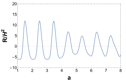
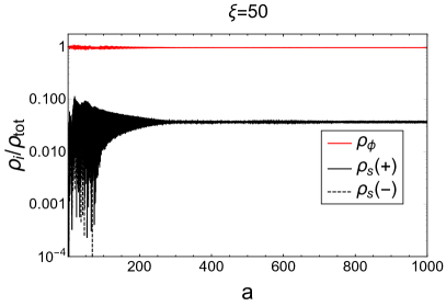
The evolution of the curvature is given by Eq. (13). Initially, it is fully determined by the zero mode of the inflaton, $R\propto 4V(\phi)-\dot{\phi}^{2}$, such that $R$ exhibits regular oscillations. This leads to coherent DM production and eventually the $\xi$–enhanced contribution of the latter to Eq. (13) becomes important. After that, the oscillations in $R$ become irregular (Fig. 2) and the resonance terminates due to backreaction of the produced particles on $R$. Thus, the end of the resonance can be associated with

$$6\xi\langle\partial^{\mu}s\partial_{\mu}s\rangle\sim 4V(\phi)\;.$$ (32)

Since the characteristic momentum squared for the tachyonic modes is $\xi R$ (see Eq. (10)), while the right hand side is of order $M_{\textrm{Pl}}^{2}R$, this condition can be rewritten as

$$\sqrt{\langle s^{2}\rangle}\sim{M_{\textrm{Pl}}\over\xi}\;.$$ (33)

Note that, at this value of $\langle s^{2}\rangle$, the function $F(s)$ starts to differ from one. For very large $\xi\gtrsim 10^{2}$, the resonance is short-lived and terminates before $a=2$. For instance, in the case $\xi=500$, the scalar curvature $R$ makes only one oscillation before turning to zero, which signifies the onset of pure radiation domination.

It is important to note that the above estimate does not give the terminal value of $\langle s^{2}\rangle$, which can increase further after the end of the resonance due to strong rescattering effects. Numerically, we find that at $\xi\gtrsim 10^{2}$, the scalar variance $\sqrt{\langle s^{2}\rangle}$ tends to the value of order $10^{-2}M_{\textrm{Pl}}$ at $a\sim 10$.

3.2.3 Large $\xi$ and significant $\lambda_{s}$

At small $\lambda_{s}$, the condition for the resonance termination remains as above, while at stronger $\lambda_{s}$, the tachyonic resonance ends when the effective DM mass turns positive. Since $s$-self-interaction induces effective mass squared of order $\lambda_{s}\langle s^{2}\rangle$ and the gravity-induced contribution is $\xi R$, we obtain the following condition

$$\xi R\sim\lambda_{s}\langle s^{2}\rangle\;.$$ (34)

The consequent $\langle s^{2}\rangle$ is of order $\xi\lambda_{\phi}\phi^{4}/(\lambda_{s}M_{\textrm{Pl}}^{2})$. This value is substantially smaller than that in the $\lambda_{s}=0$ limit if

$$\lambda_{s}\gtrsim\mathcal{O}(10^{-2}\,\xi^{3}\lambda_{\phi})\;,$$ (35)

where we have assumed that resonance terminates for $\phi$ a factor of a few below the Planck scale. Hence, condition (34) applies to this case.
 

3.3 Dark matter relic abundance

In this subsection, we study the relic abundance of dark matter generated via its non-minimal coupling to gravity. To compute it, we need to model reheating, i.e. conversion of the inflaton energy into the SM radiation. The simplest way to do it is to introduce a small trilinear inflaton coupling to the Higgs field,

$$V_{\phi h}=\sigma_{\phi h}\phi H^{\dagger}H\;.$$ (36)

This leads to perturbative inflaton decay into the Higgs pairs, as long as $m_{\phi}>2m_{h}$, and subsequent thermalization of the SM particle bath. In this case, reheating occurs at late times, when the Jordan and Einstein frames become essentially indistinguishable.

The dark matter abundance is characterized by

$$Y={n\over s_{\textrm{SM}}}~{}~{},~{}~{}s_{\textrm{SM}}={2\pi^{2}\over 45}\,g_{*s}\,T^{3}\;,$$ (37)

where $n$ is the DM number density, $s_{\textrm{SM}}$ is the Standard Model entropy density at temperature $T$ and $g_{*s}$ is the effective number of SM degrees of freedom contributing to the entropy. In our case, DM interacts very weakly and never reaches thermal equilibrium. Its particle number is approximately conserved after the preheating stage and required to match the observed abundance [39]

$$Y_{\infty}=4.4\times 10^{-10}\;\left({\textrm{GeV}\over m_{s}}\right)\;.$$ (38)

Reheating takes place when

$$H_{R}\simeq\Gamma_{\phi\rightarrow hh}\;,\quad\Gamma_{\phi\rightarrow hh}=\frac{\sigma_{\phi h}^{2}}{8\pi m_{\phi}},$$ (39)

where $H_{R}$ is the Hubble rate at reheating and $\Gamma_{\phi\rightarrow hh}$ includes 4 Higgs d.o.f. at high energies. The reheating temperature is found via

$$H_{R}=\sqrt{\frac{\pi^{2}g_{*}}{90}}\,{T_{R}^{2}\over M_{\textrm{Pl}}}\;,$$ (40)

where $g_{*}$ is the effective number of the SM degrees of freedom contributing to the energy density. Combining the above $T_{R}$ and the dark matter number density $n$ computed with the lattice simulations, one determines $Y$ according to (37).

We find that, in order to obtain the correct DM relic abundance, inflaton decay should happen in the non-relativistic regime, i.e. when the average energy per inflaton quantum is close to $m_{\phi}$. Therefore, the Universe evolution goes through a relativistic and a non-relativistic expansion phase, prior to reheating,

$$a_{e}\overset{\textrm{rel}}{\longrightarrow}a_{*}\overset{\textrm{nrel}}{\longrightarrow}a_{R}\;,$$ (41)

where $a_{e},a_{*},a_{R}$ are the scale factors associated with the end of the simulation, the onset of the non-relativistic regime and the reheating phase. In computing $a_{R}$, we approximate the equation of state of the system by $w=1/3$ in the first period and $w=0$ in the second period. As a result, we obtain the following equation for $\sigma_{\phi h}$ producing the right DM relic density [27, 26]

$$\sigma_{\phi h}\simeq 5\times 10^{-9}\;{m_{\phi}^{3/2}\over M_{\textrm{Pl}}^{1/2}}~{}{n_{e}(\phi)\over n_{e}(s)}~{}~{}\left({\textrm{GeV}\over m_{s}}\right)\;,$$ (42)

which only requires the particle densities as an output of the simulations. Here $n_{e}(\phi)$ and $n_{e}(s)$ are the particle number densities at the end of the simulation, computed by integrating the occupation numbers for all the $k$-modes (including the zero mode). At late times, the particle number and $n_{e}(\phi)/n_{e}(s)$ remain constant.

Figure 3: The couplings producing the correct DM abundance in the quartic inflaton potential with the initial condition $\Phi_{0}\simeq 0.9\,M_{\textrm{Pl}}$. The area above the curve is ruled out by overabundance of dark matter. The reheating temperature can be read off from the $y$-axis on the right. The results for other DM masses are obtained by a simple rescaling according to (42).

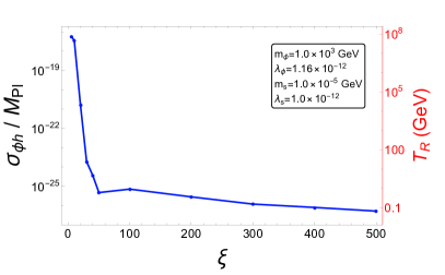
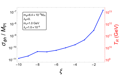
Our numerical results for $\sigma_{\phi h}$ and $T_{R}$ are shown in Fig. 3. We compute $n_{e}(\phi)$ and $n_{e}(s)$ with a version of CosmoLattice customised to include the non-minimal coupling to gravity. The simulations yield the evolution of $a(t)$ and $s(x),\phi(x)$ without resorting to the large $\xi$ approximation (as long as $\xi\gtrsim 5$), which are used to calculate the $k$-mode occupation numbers at late times. We find that these are well defined for $\lambda_{s}=10^{-12}$ and the DM particle number is conserved in this regime.

For lower $\xi\sim 10$, the DM abundance is very sensitive to the exact value of the non-minimal coupling. This is due to the exponential dependence of $n_{e}(s)$ on $\xi$. However, such sensitivity is lost at higher $\xi$. We observe that the $\sigma_{\phi h}(\xi)$ dependence flattens at $\xi>50$. This is characteristic of quasi-equilibrium, i.e. the state in which the average energy per inflaton and dark matter quanta is roughly the same and $n_{e}(\phi)/n_{e}(s)\sim\mathcal{O}(1)$. This ratio approaches one at around $\xi\sim 500$, while for yet higher values of $\xi$, the simulations become unstable. Compared to the case of a direct inflaton-DM coupling $\phi^{2}s^{2}$ [26], the system approaches exact quasi-equilibrium quite slowly with respect to $\xi$. Indeed, the dynamics in the two cases are different: the term $\xi s^{2}R$ is active only for a short time, after which the distributions of $\phi$ and $s$ evolve almost independently. In contrast, the direct coupling is active for a longer period and equilibrates the two fields more efficiently. For completeness, we also present our results for $\xi<0$, which exhibit a similar trend to those for $\xi>0$.

In Fig. 3, we choose a relatively low inflaton mass of 1 TeV. This is consistent with the bound on the reheating temperature $T_{R}>4\;$MeV [40] and the DM relic abundance only for low enough $m_{s}$, which we take to be 10 keV. Particle production after inflation is very intense such that larger $m_{s}$ would lead to DM overabundance for our parameter choice. The required $\sigma_{\phi h}$ for different $m_{s}$ can be obtained by a simple rescaling according to (42), as long as $m_{\phi}^{\textrm{}}\gg m_{s}$. At large $\xi$ corresponding to the quasi-equilibrium regime, the $m_{\phi}$-dependence also becomes simple: since $n_{e}(\phi)/n_{e}(s)\sim\mathcal{O}(1)$, the coupling $\sigma_{\phi h}$ scales as $m_{\phi}^{3/2}$.

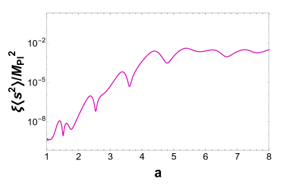
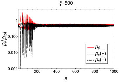
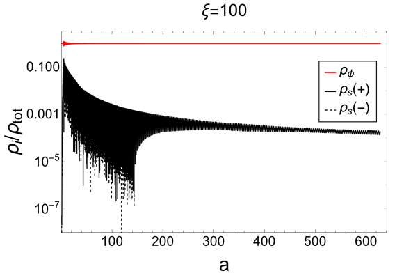
Fig. 4 illustrates the energy balance for $\xi=50$ and $\xi=500$. While DM contributes about 4% to the total energy at late times for $\xi=50$, this number goes up to 50% at $\xi=500$. We note that the DM energy density of $s$ can be negative at early times due to the scalar-graviton mixing discussed in Section 2.

Figure 4: Relative contributions of the inflaton ($\rho_{\phi}$) and dark matter ($\rho_{s}$) to the total energy density in the Jordan frame. At early times, $\rho_{s}$ can be negative (dashed line) due to the scalar-graviton mixing. At late times, the particle number is conserved.

Finally, an important feature of our scenario is that the dark sector is much ‘‘colder’’ than the observable sector. This is due to the fact that the $s$-quanta are produced immediately after inflation such that their momenta are subject to strong red-shifting. We find, in particular, that the ratio between the SM bath temperature $T_{\textrm{SM}}$ and the characteristic energy of the DM quantum $\langle E(s)\rangle$ after reheating scales as

$${T_{\textrm{SM}}\over\langle E(s)\rangle}\sim\left({1\over\lambda_{\phi}}\,{a_{R}\over a_{*}}\right)^{1/4}\gg 1\;,$$ (43)

where we have used the fact that the typical energy of the DM and inflaton quanta at preheating is of order $\sqrt{\lambda_{\phi}}\phi_{0}$. Therefore, even very light DM particles, well below a keV, become non-relativistic at the structure formation temperature of order a keV. As a result, the structure formation constraints are easily evaded.

4 Quadratic local inflaton potential

The inflaton potential around the minimum can also be dominated by the mass term,

$$V(\phi)\simeq{1\over 2}m_{\phi}^{2}\,\phi^{2}\;.$$ (44)

As $\phi(t)$ oscillates in the quadratic potential, dark matter quanta are produced via tachyonic resonance. The analysis of particle production is analogous to that in the $\phi^{4}$ case, although there are differences.

4.1 The resonance

In the $\phi^{2}$ potential, the inflaton field evolves according to

$$\phi(t)\simeq\phi_{0}\,\cos m_{\phi}t\;,$$ (45)

with slowly decreasing $\phi_{0}\propto a^{-3/2}\propto(m_{\phi}t)^{-1}$. Thus, the curvature has the form (see Eq. (17))

$$R\simeq{\phi_{0}^{2}m_{\phi}^{2}\over 2M_{\textrm{Pl}}^{2}}\,(3\cos 2m_{\phi}t+1)\;.$$ (46)

At $\lambda_{s}=0$, Eq. (21) then yields the EOM for the DM momentum modes $X_{k}$ in the form of the Mathieu equation [41],

$$X_{k}^{\prime\prime}+\left[A_{k}+2q\,\cos 4z\right]\,X_{k}=0\;,$$ (47)

where the $wH^{2}$ term has been neglected as before, the prime denotes differentiation with respect to $z=m_{\phi}t/2$ , and

$$q={3\xi\phi_{0}^{2}\over M_{\textrm{Pl}}^{2}},~{}~{}A_{k}={2\xi\phi_{0}^{2}\over M_{\textrm{Pl}}^{2}}+{4k^{2}\over a^{2}m_{\phi}^{2}}\;.$$ (48)

For the zero mode, one has $A_{0}/q=2/3$. The large $q$ regime corresponds to broad tachyonic resonance since the DM effective mass turns negative for the part of the oscillation cycle. The DM self-interaction can be taken into account in this regime using the Hartree approximation, as before, while lattice simulations allow us to go beyond it.

Figure 5: Stability charts for the Mathieu equation. Left: $\xi>0$; right: $\xi<0$. The color coding represents the Floquet exponent.

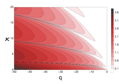
The stability chart for the Mathieu equation including the Floquet exponents is shown in Fig. 5. We observe that $q\sim 1$ leads to no exponential amplitude growth. Unlike in the quartic case, the most excited modes are the infrared ones,

$$k_{\textrm{max}}\simeq 0\;,$$ (49)

which also trivially applies to the inflaton itself. We find, however, that the spectrum of occupation numbers for tachyonic momentum modes is close to a flat one, with some IR tilt.

4.2 End of resonance

To account for collective effects in the system dynamics, we perform lattice simulations with CosmoLattice. We take the initial inflaton value to be

$$\Phi_{0}\simeq 0.9\,M_{\textrm{Pl}}$$ (50)

and its initial velocity to be zero. The benchmark inflaton mass is set to $0.6\times 10^{-5}M_{\textrm{Pl}}$. We use $\lambda_{s}=10^{-6}$ to suppress the negative energy contributions to $\rho_{s}$ at late times. Such a coupling does not lead to $s$-thermalization for any DM mass above a keV [42].

The considerations of Section 3.2 qualitatively apply to the quadratic case as well. Focussing on the positive $\xi$ case, we find that the simulations are reliable for $\xi>5$. The backreaction effects do not significantly affect the resonance for

$$\xi<75\;,$$ (51)

in which case the resonance ends due to the time evolution of the Mathieu equation coefficients, in particular, when $q$ becomes of order one. At larger $\xi$, the resonance is shut off by backreaction on the curvature, as explained in Section 3.2, which corresponds to

$$\sqrt{\langle s^{2}\rangle}\sim{M_{\textrm{Pl}}\over\xi}\;.$$ (52)

If, on the other hand, $\lambda_{s}$ is significant, the resonance can be terminated by the induced DM mass when

$$\lambda_{s}\langle s^{2}\rangle\sim\xi R\;,$$ (53)

which requires

$$\lambda_{s}\gtrsim\mathcal{O}\left(10^{-1}\,\xi^{3}{m_{\phi}^{2}\over M^{2}_{\textrm{Pl}}}\right)\;.$$ (54)

Here we have assumed that the resonance ends at $\phi$ a factor of a few below the Planck scale. For our parameter choice, this inequality is translated to $\lambda_{s}\gtrsim 10^{-6}$ at $\xi=100$. Since we set $\lambda_{s}=10^{-6}$ as our input value, the resonance is shut off by different mechanisms for $\xi$ above and below 100.

4.3 Dark matter relic abundance

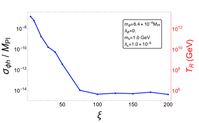
Repeating the steps put forth in Section 3.3, we compute the Higgs-inflaton coupling $\sigma_{\phi h}$ and the reheating temperature required for the correct DM relic abundance according to Eq. (42). The results are shown in Fig. 6. The main difference from the quartic case is that the matter-dominated expansion phase is much longer for the $\phi^{2}$ potential, which allows for higher $\sigma_{\phi h}$ and $T_{R}$. For our parameter choice, the inflaton-DM system scales as non-relativistic matter, so $a_{e}=a_{*}$.

For moderate $\xi$, the relic abundance is exponentially sensitive to the value of the non-minimal coupling. At $\xi\sim 75$, the right panel of Fig. 6 exhibits a transition to qualitatively different behaviour. For larger $\xi$, the $\sigma_{\phi h}$ curve flattens and the system slowly approaches quasi-equilibrium, although $n(\phi)/n(s)\sim 10^{2}$ still at this stage.

For completeness, in the left panel of Fig. 6, we present some of our results for $\xi<0$. The simulation assumes vacuum initial conditions for the DM fluctuations, which may not be a good approximation for negative $\xi$ in simple set-ups. Nevertheless, this may be appropriate for more complicated multi-field inflationary models, where some fields have direct couplings to $s$. We find that the classical dynamics approach is valid for $\xi<-1$, yet we have not been able to obtain reliable results for $\xi<-10$ due to the large Floquet exponents and persistent presence of negative energies.

Figure 6: Couplings and reheating temperature producing the correct DM abundance in the quadratic inflaton potential with $\Phi_{0}\simeq 0.9\,M_{\textrm{Pl}}$. The area above the curve is ruled out by overabundance of dark matter. The results for other DM masses are obtained by a simple rescaling according to (42).

The negative energy issue becomes more significant in the $\phi^{2}$ potential case. This is because the unwanted contribution to $\rho_{s}$ is proportional to $H\propto a^{-3/2}$, which decreases slower than it did in the $\phi^{4}$ potential. As a result, a larger $\lambda_{s}$ and/or longer running time is needed to obtain meaningful occupation numbers. This tendency is seen in Fig. 7, which shows that negative energies appear until $a\sim 150$ even for $\lambda_{s}=10^{-6}$. Eventually, the induced mass contribution regularizes this behaviour since $\lambda_{s}\langle s^{2}\rangle^{2}$ decreases slower than $\xi H\langle s\dot{s}\rangle$ does. For $\xi<0$, on the other hand, there is an additional negative contribution $\xi H^{2}\langle s^{2}\rangle$ to the DM energy density, which makes the analysis more time consuming and computer-intensive.

We observe that, after the end of the resonance, dark matter takes up to 20% of the energy density of the system for $\xi=100$. Its contribution scales as radiation, so this fraction decreases over time, unlike that in the $\phi^{4}$ case. As $\xi$ increases, quasi-equilibrium is approached very slowly since the inter-species interaction is only significant at early times. Although this trend is visible, we have not identified the coupling $\xi$ necessary for the exact quasi-equilibrium, at least for the parameters at hand.

It should be noted that our DM abundance predictions become less reliable at large $\sigma_{\phi h}$, around $10^{-8}M_{\textrm{Pl}}$. At such coupling values, early time Higgs production due to the tachyonic resonance becomes significant since $\sigma_{\phi h}\Phi_{0}/m_{\phi}^{2}\gg 1$. On the other hand, the energy transfer to the Higgs field is small due to strong backreaction induced by the Higgs self-coupling $\lambda_{h}\sim 10^{-2}$. It will further be diluted by matter-dominated expansion such that we expect our results to give the right ballpark answer. Related lattice studies of the $\sigma_{\phi h}$-induced resonance were performed in [43], although with the assumption of $\lambda_{h}<0$ at high energy. This analysis would be altered dramatically by backreaction for $\lambda_{h}\sim+10^{-2}$, as an example presented in [14] shows.

Figure 7: Energy balance $\rho_{i}/\rho_{\textrm{tot}}$ in the inflaton-DM system at $\xi=100$, $\lambda_{s}=10^{-6}$. The dashed line represents negative $\rho_{s}$ appearing due to the scalar-graviton mixing. At late times, the particle number is conserved.

5 Conclusion

We have studied dark matter production via its non-minimal coupling to gravity $\xi s^{2}R$ in both (locally) quadratic and quartic inflaton potentials. We find that collective effects such as backreaction and rescattering make an important impact on the dark matter abundance, especially at large couplings $\xi>30$. The system tends to quasi-equilibrium at yet larger $\xi>100$, in which case the DM abundance becomes almost independent of $\xi$. We also find that although the Jordan frame energy density of scalar DM can be negative, its late time behaviour is sensible, at least in the presence of a small self-coupling, which allows one to define a meaningful, conserved particle number in this regime. The dark matter production mechanism is very efficient, originating from tachyonic resonance, and leads to the correct DM abundance for a wide range of DM masses.

The mechanism considered in this paper constitutes one of possible gravitational channels for dark matter production. The non-minimal coupling to curvature can be eliminated by a metric transformation in favor of higher dimensional inflaton-dark matter couplings in the Einstein frame. Such operators are also expected to be generated directly by quantum gravitational effects [27, 44], which creates a significant uncertainty in the DM abundance calculations. In the present work, we focus entirely on the effect of the non-minimal coupling to curvature, although a UV complete model would have multiple sources of dark matter production.
 
Acknowledgements. We are grateful to the authors of [28], especially D. Figueroa and A. Florio, for providing us with an upgraded version of CosmoLattice. We also wish to thank the Finnish Grid and Cloud Infrastructure (FGCI) for supporting this project with computational and data storage resources. J.Y. would like to thank the lecturers and participants of CosmoLattice School 2022 for sharing their expertise that assisted the research presented in this work. J.Y. also acknowledges helpful discussions with Yann Mambrini, Simon Cléry, and Essodjolo Kpatcha. We acknowledge support by Institut Pascal at Université Paris-Saclay during the Paris-Saclay Astroparticle Symposium 2022, with the support of the P2IO Laboratory of Excellence (program ‘‘Investissements d’avenir’’ ANR-11-IDEX-0003-01 Paris-Saclay and ANR-10-LABX-0038), the P2I axis of the Graduate School of Physics of Université Paris-Saclay, as well as IJCLab, CEA, APPEC, IAS, OSUPS, and the IN2P3 master projet UCMN.

References

- [1] A. A. Starobinsky, A New Type of Isotropic Cosmological Models Without Singularity, Phys. Lett. B 91 (1980), 99-102,
- [2] A. H. Guth, The Inflationary Universe: A Possible Solution to the Horizon and Flatness Problems, Phys. Rev. D 23 (1981), 347-356
- [3] A. D. Linde, A New Inflationary Universe Scenario: A Possible Solution of the Horizon, Flatness, Homogeneity, Isotropy and Primordial Monopole Problems, Phys. Lett. B 108 (1982), 389-393
- [4] A. D. Linde, Chaotic Inflation, Phys. Lett. B 129 (1983), 177-181
- [5] V. F. Mukhanov and G. V. Chibisov, Quantum Fluctuations and a Nonsingular Universe, JETP Lett. 33 (1981), 532-535
- [6] L. Parker, Quantized fields and particle creation in expanding universes. 1., Phys. Rev. 183 (1969), 1057-1068
- [7] A. A. Grib and S. G. Mamaev, On field theory in the friedman space, Yad. Fiz. 10 (1969), 1276-1281
- [8] A. D. Dolgov and D. P. Kirilova, On particle creation by a time dependent scalar field, Sov. J. Nucl. Phys. 51 (1990), 172-177
- [9] J. H. Traschen and R. H. Brandenberger, Particle Production During Out-of-equilibrium Phase Transitions, Phys. Rev. D 42 (1990), 2491-2504
- [10] L. H. Ford, Cosmological particle production: a review, Rept. Prog. Phys. 84 (2021) no.11, 116901, [2112.02444]
- [11] O. Lebedev, The Higgs portal to cosmology, Prog. Part. Nucl. Phys. 120 (2021), 103881, [2104.03342]
- [12] N. A. Chernikov and E. A. Tagirov, Quantum theory of scalar fields in de Sitter space-time, Ann. Inst. H. Poincare Phys. Theor. A 9 (1968), 109
- [13] I. L. Buchbinder, S. D. Odintsov and I. L. Shapiro, Effective action in quantum gravity, CRC Press, 1992
- [14] O. Lebedev and J. H. Yoon, Challenges for inflaton dark matter, Phys. Lett. B 821 (2021), 136614, [2105.05860]
- [15] B. A. Bassett and S. Liberati, Geometric reheating after inflation, Phys. Rev. D 58 (1998), 021302, [erratum: Phys. Rev. D 60 (1999), 049902], [hep-ph/9709417]
- [16] S. Tsujikawa, K. i. Maeda and T. Torii, Preheating with nonminimally coupled scalar fields in higher curvature inflation models, Phys. Rev. D 60 (1999), 123505, [hep-ph/9906501]
- [17] O. Bertolami, P. Frazao and J. Paramos, Reheating via a generalized non-minimal coupling of curvature to matter, Phys. Rev. D 83 (2011), 044010, [1010.2698]
- [18] N. Koivunen, E. Tomberg and H. Veermäe, The linear regime of tachyonic preheating, JCAP 07 (2022) no.07, 028, [2201.04145]
- [19] T. Markkanen and S. Nurmi, Dark matter from gravitational particle production at reheating, JCAP 02 (2017), 008, [1512.07288]
- [20] M. Fairbairn, K. Kainulainen, T. Markkanen and S. Nurmi, Despicable Dark Relics: generated by gravity with unconstrained masses, JCAP 04 (2019), 005, [1808.08236]
- [21] J. A. R. Cembranos, L. J. Garay and J. M. Sánchez Velázquez, Gravitational production of scalar dark matter, JHEP 06 (2020), 084, [1910.13937]
- [22] E. Babichev, D. Gorbunov, S. Ramazanov and L. Reverberi, Gravitational reheating and superheavy Dark Matter creation after inflation with non-minimal coupling, JCAP 09 (2020), 059, [2006.02225]
- [23] S. Clery, Y. Mambrini, K. A. Olive, A. Shkerin and S. Verner, Gravitational portals with nonminimal couplings, Phys. Rev. D 105 (2022) no.9, 095042, [2203.02004]
- [24] O. Catà, A. Ibarra and S. Ingenhütt, Dark matter decays from nonminimal coupling to gravity, Phys. Rev. Lett. 117 (2016) no.2, 021302, [1603.03696]
- [25] K. Kainulainen, O. Koskivaara and S. Nurmi, Tachyonic production of dark relics: a non-perturbative quantum study, [2209.10945]
- [26] O. Lebedev, F. Smirnov, T. Solomko and J. H. Yoon, Dark matter production and reheating via direct inflaton couplings: collective effects, JCAP 10 (2021) 032, [2107.06292]
- [27] O. Lebedev and J. H. Yoon, On gravitational preheating, JCAP 07 (2022) no.07, 001, [2203.15808]
- [28] D. G. Figueroa, A. Florio, T. Opferkuch and B. A. Stefanek, Dynamics of Non-minimally Coupled Scalar Fields in the Jordan Frame, [2112.08388]
- [29] D. S. Salopek, J. R. Bond and J. M. Bardeen, Designing Density Fluctuation Spectra in Inflation, Phys. Rev. D 40 (1989), 1753
- [30] G. N. Felder, J. Garcia-Bellido, P. B. Greene, L. Kofman, A. D. Linde and I. Tkachev, Dynamics of symmetry breaking and tachyonic preheating, Phys. Rev. Lett. 87 (2001), 011601, [hep-ph/0012142]
- [31] P. B. Greene, L. Kofman, A. D. Linde and A. A. Starobinsky, Structure of resonance in preheating after inflation, Phys. Rev. D 56 (1997), 6175-6192, [hep-ph/9705347]
- [32] D. Polarski and A. A. Starobinsky, Semiclassicality and decoherence of cosmological perturbations, Class. Quant. Grav. 13 (1996), 377-392, [gr-qc/9504030]
- [33] D. G. Figueroa, A. Florio, F. Torrenti and W. Valkenburg, The art of simulating the early Universe – Part I, JCAP 04 (2021), 035, [2006.15122]
- [34] D. G. Figueroa, A. Florio, F. Torrenti and W. Valkenburg, CosmoLattice, Comput. Phys. Commun. 283 (2023), 108586, [2102.01031]
- [35] https://cosmolattice.net/
- [36] D. Bettoni, A. Lopez-Eiguren and J. Rubio, Hubble-induced phase transitions on the lattice with applications to Ricci reheating, JCAP 01 (2022) no.01, 002, [2107.09671]
- [37] Y. Ema, M. Karciauskas, O. Lebedev and M. Zatta, Early Universe Higgs dynamics in the presence of the Higgs-inflaton and non-minimal Higgs-gravity couplings, JCAP 06 (2017), 054, [1703.04681]
- [38] Q. Li, T. Moroi, K. Nakayama and W. Yin, Instability of the electroweak vacuum in Starobinsky inflation, JHEP 09 (2022), 102, [2206.05926]
- [39] P. A. R. Ade et al. [Planck], Planck 2015 results. XIII. Cosmological parameters, Astron. Astrophys. 594 (2016), A13, [1502.01589]
- [40] S. Hannestad, What is the lowest possible reheating temperature?, Phys. Rev. D 70 (2004), 043506, [astro-ph/0403291]
- [41] L. Kofman, A. D. Linde and A. A. Starobinsky, Towards the theory of reheating after inflation, Phys. Rev. D 56 (1997), 3258-3295, [hep-ph/9704452]
- [42] G. Arcadi, O. Lebedev, S. Pokorski and T. Toma, Real Scalar Dark Matter: Relativistic Treatment, JHEP 08 (2019), 050, [1906.07659]
- [43] K. Enqvist, M. Karciauskas, O. Lebedev, S. Rusak and M. Zatta, Postinflationary vacuum instability and Higgs-inflaton couplings, JCAP 11 (2016), 025, [1608.08848]
- [44] O. Lebedev, Scalar overproduction in standard cosmology and predictivity of non-thermal dark matter, [2210.02293]