The Rumble in the Meson:
a leptoquark versus a $Z^{\prime}$
to fit $b\rightarrow s\mu^{+}\mu^{-}$ anomalies
including 2022 LHCb $R_{K^{(\ast)}}$ measurements

Abstract

We juxtapose global fits of two bottom-up models (an $S_{3}$ scalar leptoquark model and a ${B_{3}-L_{2}}$ $Z^{\prime}$ model) of $b\rightarrow s\mu^{+}\mu^{-}$ anomalies to flavour data in order to quantify statistical preference or lack thereof. The leptoquark model couples directly to left-handed di-muon pairs, whereas the $Z^{\prime}$ model couples to di-muon pairs with a vector-like coupling. $B_{s}-\overline{B_{s}}$ mixing is a focus because it is typically expected to disfavour $Z^{\prime}$ explanations. In two-parameter fits to 247 flavour observables, including $B_{s/d}\to\mu^{+}\mu^{-}$ branching ratios for which we provide an updated combination and LHCb $R_{K^{(\ast)}}$ measurements from December 2022, we show that each model provides a similar improvement in quality-of-fit of $\sqrt{\Delta\chi^{2}}=3.6$ with respect to the Standard Model. The main effect of the $B_{s}-\overline{B_{s}}$ mixing constraint in the $Z^{\prime}$ model is to disfavour values of the $s_{L}-b_{L}$ mixing angle greater than about $5|V_{cb}|$. This limit is rather loose, meaning that a good fit to data does not require ‘alignment’ in either quark Yukawa matrix. No curtailment of the $s_{L}-b_{L}$ mixing angle is evident in the $S_{3}$ model.

1 Introduction

Tensions between Standard Model (SM) predictions and measurements of some neutral current flavour-changing $B-$meson decays persist. We collectively call these tensions the $b\rightarrow s\mu^{+}\mu^{-}$ anomalies. For example, various lepton flavour universality (LFU) observables like the ratios of branching ratios $R_{K^{(\ast)}}=BR(B\rightarrow K^{(\ast)}\mu^{+}\mu^{-})/BR(B\rightarrow K^{(\ast)}e^{+}e^{-})$ were, prior to December 2022, measured to be lower than their SM predictions in multiple channels and several bins of di-lepton invariant mass squared LHCb:2017avl ; LHCb:2019hip ; LHCb:2021trn . Measurements of other similar ratios in $B^{0}\rightarrow K^{0}_{s}\ell^{+}\ell^{-}$ and $B^{\pm}\rightarrow K^{\ast\pm}\ell^{+}\ell^{-}$ decays LHCb:2021lvy (where $\ell\in\{e,\mu\}$) are compatible with a concomitant deficit in the di-muon channel as compared to the di-electron channel, although we note that the statistics are diminished in the $K_{s}^{0}$ and ${K^{\ast}}^{\pm}$ channels and the tension is not significant in them (it is around the 1$\sigma$ level only). SM predictions of all of the double ratios mentioned above enjoy rather small theoretical uncertainties due to their cancellation between numerator and denominator in each case for the di-lepton invariant mass squared bins of interest, such that they are robust. We include all of the aforementioned observables in the ‘LFU’ category, following the computer program smelli2.3.2 Aebischer:2018iyb that we shall use to calculate them. In December 2022, LHCb released a reanalysis of the $R_{K^{(\ast)}}$ measurements including experimental systematic effects that were missing from the previous analysis and a tighter selection of electrons. LHCb has decreed that the reanalysis supplants previous results. The reanalysis implies that the four measurements of $R_{K^{(\ast)}}$ are actually compatible with SM predictions LHCb:2022qnv , contrary to LHCb’s previous analyses.

After much theoretical work, $\overline{BR}(B_{s}\rightarrow\mu^{+}\mu^{-})$ also has quite small theoretical uncertainties in its SM prediction but, together with the correlated measurement of $BR(B\rightarrow\mu^{+}\mu^{-})$, it displays a 1.6$\sigma$ tension with a combination of the experimental measurements ATLAS:2018cur ; CMS-PAS-BPH-21-006 ; LHCb:2017rmj . Several other observables in $B-$meson decays appear to be in significant tension with SM measurements even when one takes into account their larger theoretical uncertainties, for example $BR(B^{+}\rightarrow K^{+}\mu^{+}\mu^{-})$ LHCb:2014cxe ; Parrott:2022rgu , $BR(B_{s}\rightarrow\phi\mu^{+}\mu^{-})$ LHCb:2015wdu ; CDF:2012qwd and angular distributions in $B\rightarrow K^{\ast}\mu^{+}\mu^{-}$ decays LHCb:2013ghj ; LHCb:2015svh ; ATLAS:2018gqc ; CMS:2017rzx ; CMS:2015bcy ; Bobeth:2017vxj . For these quantities, which are put in the ‘quarks’ category of observable, there is room for argument about the best predictions and the size of the associated theoretical uncertainties Gubernari:2022hxn .

category	$n_{obs}$	$\chi^{2}_{SM}$	$p$	$s/\sigma$
‘quarks’	224	262.9 259.1 (261.2)	.038 .054 (.044)	2.1 2.0 (2.0)
‘LFU’	23	17.1 39.4 (39.4)	.80 .018 (.018)	0.2 2.4 (2.4)
combined	247	280.0 298.5 (300.7)	.073 .014 (.011)	1.8 2.5 (2.5)

Table 1: SM quality-of-fit as calculated by smelli2.3.2 with an updated $\overline{BR}(B_{s}\rightarrow\mu^{+}\mu^{-})$ constraint (see §4.1). Only the values in bold include the 2022 LHCb measurements of $R_{K^{(\ast)}}$ LHCb:2022qnv and values in parentheses are obtained without updating the $\overline{BR}(B_{s}\rightarrow\mu^{+}\mu^{-})$ constraint. $n_{obs}$ shows the number of observables in each category. $\chi^{2}_{SM}$ denotes the $\chi^{2}$ statistic within each category, $p$ is the $p-$value of the category, and $s$ is the equivalent two-sided ‘number of $\sigma$’ away from the central value of a univariate normal distribution. The category ‘LFU’ contains lepton flavour universality violating flavour changing observables such as $R_{K}^{(\ast)}$, where theoretical uncertainties are relatively small. The ‘quarks’ category contains other flavour-changing $b$ observables, some of which have large theoretical uncertainties (which are nevertheless taken into account in the calculation of $\chi^{2}$).

We display the current state-of-play as regards the tensions in Table 1, as well as the change from including the LHCb measurements of $R_{K^{(\ast)}}$; the upshot is that the SM currently possesses a 1.8$\sigma$ tension with 247 combined measurements of $b\rightarrow s$ flavour-changing observables. The December 2022 LHCb measurements have decreased this from 2.5$\sigma$. We note here that the preselected 247 measurements include several observables which do not involve the $(\bar{b}s)(\bar{\mu}\mu)$ effective vertex and which also do not display large tensions, diluting (i.e. raising) the $p-$value and therefore decreasing $s/\sigma$. In an analysis which concentrates more specifically on the fewer $b\rightarrow s\mu^{+}\mu^{-}$ anomaly observables on data in 2021, an estimate of $s=4.3\sigma$ was made Isidori:2021vtc . We parenthetically observe from the table that in the context of our SM global fit to many observables, the update to the $\overline{BR}(B_{s}\rightarrow\mu^{+}\mu^{-})$ constraint has only a small effect on the quality-of-fit.

Prior to December 2022, it was well known in the literature that two-parameter new physics models can decrease $\chi^{2}$ by some 30 or so units Alguero:2021anc ; Altmannshofer:2021qrr ; Ciuchini:2020gvn ; Hurth:2021nsi resulting in a significantly better fit than the SM. One can take the two parameters to be weak effective theory (WET) Wilson coefficients (WCs), defined via the WET Hamiltonian density

$${\mathcal{H}}_{\mathrm{WET}}=-\frac{4G_{F}}{\sqrt{2}}\sum_{i}(C_{i}^{\text{SM}}+C_{i})\mathcal{O}_{i}+\text{H.c.},$$ (1)

where $C_{i}$ here denotes the beyond the SM contribution to the WC, $G_{F}$ is the Fermi decay constant and $C_{i}^{\text{SM}}$ denotes the SM contribution to the WC. The two dimension-6 operators $\mathcal{O}_{i}$ that can best ameliorate the $b\rightarrow s\mu^{+}\mu^{-}$ fits are Alguero:2021anc ; Altmannshofer:2021qrr ; Ciuchini:2020gvn ; Hurth:2021nsi

$$\mathcal{O}_{9} =\frac{e^{2}}{16\pi^{2}}\left(\bar{s}\gamma_{\mu}P_{L}b\right)\left(\bar{\mu}\gamma^{\mu}\mu\right),$$

$$\mathcal{O}_{10} =\frac{e^{2}}{16\pi^{2}}\left(\bar{s}\gamma_{\mu}P_{L}b\right)\left(\bar{\mu}\gamma^{\mu}\gamma_{5}\mu\right),$$ (2)

where $P_{L}$ is a left-handed projection operator in spinor space and $e$ is the electromagnetic gauge coupling. Here $s$, $b$ and $\mu$ are 4-component Dirac spinor fields of the strange quark, the bottom quark and the muon, respectively. In Ref. Greljo:2022jac (Fig. 1), it was shown that the LHCb 2022 reanalysis of $R_{K^{(\ast)}}$ introduces a mild $1-2\sigma$ tension between the ‘quarks’ category and ‘LFU’ category of observable, if they are interpreted only in terms of $C_{9}$ and $C_{10}$. Despite this, we find that models which predict non-zero $C_{9}$ and $C_{10}$ still provide an improved fit to the combination of current flavour data as compared to the SM.

There are two categories of beyond the SM fields that can explain the $b\rightarrow s\mu^{+}\mu^{-}$ anomalies at tree level in quantum field theory: leptoquarks, which are colour triplet scalar or vector bosons (with various possible electroweak quantum numbers), and $Z^{\prime}$s, which are SM-neutral vector bosons. In each category, the new state must have family non-universal interactions, coupling to $\overline{b_{L}}$ and $s_{L}$. The observables in which the measurements are in tension with SM predictions involve di-muon pairs. The new physics state should therefore certainly couple to di-muon pairs, but in order to agree with the December 2022 LHCb measurements $R_{K}$ and $R_{K^{\ast}}$, one may also couple it to di-electron pairs with a similar strength, although then the scenario may become strongly constrained by LEP constraints Greljo:2022jac . For the coupling to di-muon pairs, fits to flavour data by different groups agree that the new physics state should couple to left-handed di-muons. There is a preference from the data for a coupling to muons and fits to flavour data by different groups agree that the new physics state should couple to left-handed di-muons. (A purely left-handed coupling to muons realises the limit $C_{9}=-C_{10}$, which will be a prediction of the benchmark leptoquark model that we examine.) However, depending upon the treatment of the predictions of observables in the ‘quarks’ category, the different fits may or may not have a mild preference Egede:2022rxc for the new physics field to couple to right-handed di-muons in addition with a similar strength to the coupling to left-handed di-muons (e.g. realising the limit where $C_{9}\neq 0$ but $C_{10}=0$; this will be the prediction of the benchmark $Z^{\prime}$ model which we shall choose) Allanach:2020kss .

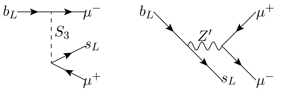
Figure 1: Tree-level Feynman diagrams of the new physics contributions to the $b\rightarrow s\mu^{+}\mu^{-}$ observables in a suitable scalar $S_{3}$ leptoquark model (left panel) and in a suitable $Z^{\prime}$ model (right panel).

We display example Feynman diagrams contributing to $b\rightarrow s\mu^{+}\mu^{-}$ processes for a scalar leptoquark and for a $Z^{\prime}$ in Fig. 1.

On the model building side, leptoquark explanations for the $b\rightarrow s\mu^{+}\mu^{-}$ anomalies have received a lot of attention. For scalar leptoquarks, only the $S_{3}\sim{\bf(\overline{3},3)}_{1/3}$ leptoquark can fit the $b\rightarrow s\mu^{+}\mu^{-}$ anomaly data Hiller:2017bzc ; Angelescu:2018tyl ; Angelescu:2021lln . Theoretical challenges include explaining why the scalar leptoquark should be as light as the TeV scale, which can be addressed in the partial compositeness framework Gripaios:2009dq ; Gripaios:2014tna , and explaining why the leptoquark does not have baryon-number violating or lepton flavour violating (LFV) couplings. The latter can be achieved by gauging an additional symmetry Davighi:2020qqa ; Greljo:2021xmg ; Greljo:2021npi ; Davighi:2022qgb , extending previous work using (global) flavour symmetries deMedeirosVarzielas:2015yxm ; Heeck:2022znj . For vector leptoquarks, a $U_{1}\sim{\bf(3,1)}_{2/3}$ or a $U_{3}\sim{\bf(3,3)}_{2/3}$ leptoquark can significantly ameliorate the quality-of-fit of the SM Angelescu:2018tyl ; Angelescu:2021lln , but a simplified model is non-renormalisable and so a ultra-violet (UV) complete model is needed. In the case of the $U_{1}$ leptoquark, a suitable class of extensions of the SM gauge group based on the ‘4321’ gauge group $SU(4)\times SU(3)\times SU(2)\times U(1)$ was invented DiLuzio:2017vat ; DiLuzio:2018zxy ; Greljo:2018tuh , which has inspired much further work. A family-triplet leptoquark model can successfully fit all data including the December 2022 LHCb $R_{K}$ measurements Greljo:2022jac .

Similarly, many $Z^{\prime}$ models have been constructed which also significantly improve the SM’s poor quality-of-fit. Many are based on spontaneously broken anomaly-free $U(1)_{X}$ gauge extensions of the SM that yield such a $Z^{\prime}$, for various choices of $X$. Examples include gauged muon minus tau lepton number $X=L_{\mu}-L_{\tau}$ Altmannshofer:2014cfa ; Crivellin:2015mga ; Crivellin:2015lwa ; Crivellin:2015era ; Altmannshofer:2015mqa , for which the required $Z^{\prime}$ coupling to $\bar{s}_{L}b_{L}$ is mediated via mixing with heavy vector-like quarks, third family baryon number minus muon lepton number $X=B_{3}-L_{2}$ Alonso:2017uky ; Bonilla:2017lsq ; Allanach:2020kss , third family hypercharge $X=Y_{3}$ Allanach:2018lvl ; Davighi:2019jwf ; Allanach:2019iiy ; Allanach:2021kzj , and other assignments Sierra:2015fma ; Celis:2015ara ; Greljo:2015mma ; Falkowski:2015zwa ; Chiang:2016qov ; Boucenna:2016wpr ; Boucenna:2016qad ; Ko:2017lzd ; Alonso:2017bff ; Tang:2017gkz ; Bhatia:2017tgo ; Fuyuto:2017sys ; Bian:2017xzg ; King:2018fcg ; Duan:2018akc ; Kang:2019vng ; Calibbi:2019lvs ; Altmannshofer:2019xda ; Capdevila:2020rrl ; Davighi:2021oel ; Allanach:2022bik . An attempt to fit the post-December 2022 data using a lepton-flavour-universal $3B_{3}-L$ data was made in Ref. Greljo:2022jac , but the model was found to be in significant tension with LEP Drell-Yan constraints coming from $e^{+}e^{-}\to\ell^{+}\ell^{-}$.

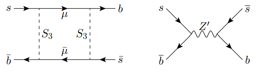
Figure 2: Example leading order Feynman diagrams of beyond the SM contribution to $B_{s}-\overline{B_{s}}$ mixing via the $S_{3}$ leptoquark (left panel) or the ${B_{3}-L_{2}}$ $Z^{\prime}$ model (right panel).

The primary aim of this paper is to compare global fits to current data of a leptoquark model with those of a $Z^{\prime}$ model. We pick two simple and comparable benchmark models that have been studied in previous literature. They shall be defined in the next Section. While current tensions in semi-leptonic $b\rightarrow s\mu^{+}\mu^{-}$ transitions between measurements and SM predictions can be ameliorated by either a leptoquark or a $Z^{\prime}$, it is anticipated that the $\Delta M_{s}$ observable King:2019lal , which parameterises $B_{s}-\overline{B_{s}}$ mixing and does not exhibit a significant tension with the SM prediction, has the power to discriminate between leptoquark and $Z^{\prime}$ explanations. Because the $Z^{\prime}$ model predicts tree-level contributions to $\Delta M_{s}$, while the dominant contributions from the leptoquark are at one-loop order (see Fig. 2) and therefore suppressed, one generically expects the constraints from $\Delta M_{s}$ to be stronger for $Z^{\prime}$ models. However, the extent of the impact of this observable on the fits should be evaluated quantitatively in each model for comparison. A secondary goal of the present paper is to examine the impact of the December 2022 LHCb measurements of $R_{K^{(\ast)}}$.

For both the leptoquark and the $Z^{\prime}$, we choose to focus on TeV-scale masses so that the models can avoid the bounds originating from direct searches at the LHC. For TeV-scale masses, the new physics state’s contribution to the anomalous magnetic moment of the muon $(g-2)_{\mu}$ is negligible without augmenting the model with additional fields Allanach:2015gkd and so we exclude this observable from our fits.

In each model, we do expect there to be additional fields that we (usually) shall assume have a negligible effect upon the $b\rightarrow s\mu^{+}\mu^{-}$ observables either because they are too weakly coupled or because they are too heavy. For example, additional heavy fermionic fields are expected in order to generate SM-fermion mixing. If additional fermionic fields are added in vector-like representations of the gauge group, then the model remains anomaly free and large masses for said fermions are allowed by the gauge symmetry. Additional fields could be added in order to explain the current tension in $(g-2)_{\mu}$, for example additional vector-like leptons Allanach:2015gkd , where a one-loop diagram with a $Z^{\prime}$ along with additional leptons in the loop can resolve it. Other heavy fields associated with dark matter could also be added. Here, our effective quantum field theory is supposed to be valid at and below the scale of the mass of the $Z^{\prime}$ or leptoquark state, i.e. the TeV scale, and we assume that the effect of other heavy fields on the pertinent flavour phenomenology is negligible.

The parameter space of the ${B_{3}-L_{2}}$ $Z^{\prime}$ model model was adapted to $b\rightarrow s\mu^{+}\mu^{-}$ data and various phenomenological constraints were applied in Refs. Alonso:2017uky ; Bonilla:2017lsq ; Allanach:2020kss ; Allanach:2021gmj . Some more recent flavour data and LHC $Z^{\prime}$ search limits were employed to constrain the model in Ref. Azatov:2022itm . In that reference, similar constraints were also applied to the $S_{3}$ leptoquark model (estimated before with earlier data by Refs. Allanach:2017bta ; Allanach:2019zfr ), before calculating future collider sensitivities of the two models. In all of these prior works, the parameters of each model were fit to central values for $C_{9}$ and $C_{10}$ obtained from fits to $b\to s\ell^{+}\ell^{-}$ data, assuming that all other SM effective field theory (SMEFT) operators were zero. The additional constraints, including those from meson mixing and LHC searches, were individually applied to obtain 95$\%$ CL bounds. The bottom line of Ref. Azatov:2022itm relevant for the present paper is that, in each model, there is a sizeable parameter space that evades current search limits and satisfies other phenomenological constraints, and that simultaneously explains the $b\rightarrow s\mu^{+}\mu^{-}$ anomalies. In the present paper we go beyond the prior studies by performing a side-by-side global flavour fit of each model to identical empirical datasets. All dimension-6 SMEFT operators are included – not just those that generate $C_{9}$ and $C_{10}$ – including 4-quark and 4-lepton operators induced at tree-level in the $Z^{\prime}$ model, and those operator contributions generated by one-loop renormalisation effects. We then perform a goodness-of-fit test on each model, comparing the best-fit points to quantify any statistical preference of the data for either model.

The paper proceeds as follows: §2, we introduce the $S_{3}$ leptoquark model and the ${B_{3}-L_{2}}$ $Z^{\prime}$ model. In order to make further progress, some assumptions about fermion mixing must be made and we lay these out first; they are identical for each of the two models. In §3 we present the matching to the WCs of dimension-6 operators in the SMEFT resulting from integrating out the new physics state. The fit to each model will be described by 2 effective parameters extra to the SM. For given values of these parameters, the dimension-6 SMEFT operator WCs are then given and can be passed as input to smelli2.3.2, which calculates the observables and quality-of-fit. Fit results are presented in §4, where we shall observe that the leptoquark model has a similar quality-of-fit as the $Z^{\prime}$ model, indicating that the $\Delta M_{s}$ observable was less discriminating than one might have expected. We summarise and conclude in §5.

2 Models

It is our purpose here to add a TeV-scale new physics field to the SM with couplings that facilitate an explanation of the $b\rightarrow s\mu^{+}\mu^{-}$ anomalies. We will not develop the model-building fully into the UV, being content to describe the important phenomenology such that experimental assessments of the $b\rightarrow s\mu^{+}\mu^{-}$ anomalies can be made. We begin by writing down our conventions as regards fermion mixing, since they are common to both the $S_{3}$ model and the ${B_{3}-L_{2}}$ $Z^{\prime}$ model.

2.1 Fermion mixing conventions

In the fermionic fields’ gauge eigenbasis, which we indicate via ‘primed’ symbols, we write

$${\bf u_{L}^{\prime}} = \left(\begin{array}[]{c}u_{L}^{\prime}\\ c_{L}^{\prime}\\ t_{L}^{\prime}\\ \end{array}\right),\qquad{\bf d_{L}^{\prime}}=\left(\begin{array}[]{c}d_{L}^{\prime}\\ s_{L}^{\prime}\\ b_{L}^{\prime}\\ \end{array}\right),\qquad{\bf e_{L}^{\prime}}=\left(\begin{array}[]{c}e_{L}^{\prime}\\ \mu_{L}^{\prime}\\ \tau_{L}^{\prime}\\ \end{array}\right),\qquad{\bm{\nu}_{L}^{\prime}}=\left(\begin{array}[]{c}{\nu_{e}^{\prime}}_{L}\\ {\nu_{\mu}^{\prime}}_{L}\\ {\nu_{\tau}^{\prime}}_{L}\\ \end{array}\right),$$ (15)

$${\bf u_{R}^{\prime}} = \left(\begin{array}[]{c}u_{R}^{\prime}\\ c_{R}^{\prime}\\ t_{R}^{\prime}\\ \end{array}\right),\qquad{\bf d_{R}^{\prime}}=\left(\begin{array}[]{c}d_{R}^{\prime}\\ s_{R}^{\prime}\\ b_{R}^{\prime}\\ \end{array}\right),\qquad{\bf e_{R}^{\prime}}=\left(\begin{array}[]{c}e_{R}^{\prime}\\ \mu_{R}^{\prime}\\ \tau_{R}^{\prime}\\ \end{array}\right),\qquad{\bm{\nu}_{R}^{\prime}}=\left(\begin{array}[]{c}{\nu_{e}^{\prime}}_{R}\\ {\nu_{\mu}^{\prime}}_{R}\\ {\nu_{\tau}^{\prime}}_{R}\\ \end{array}\right),$$ (28)

along with the SM fermionic electroweak doublets

$${\bf Q^{\prime}}_{i}=\left(\begin{array}[]{c}{\bf u_{L}^{\prime}}_{i}\\ {\bf d_{L}^{\prime}}_{i}\end{array}\right),\qquad{\bf L^{\prime}}_{i}=\left(\begin{array}[]{c}{\bm{\nu}_{L}^{\prime}}_{i}\\ {\bf e_{L}^{\prime}}_{i}\end{array}\right).$$ (29)

The SM fermions acquire masses after the SM Brout-Englert-Higgs mechanism through

$$-\mathcal{L}_{Y} = \overline{\bf Q^{\prime}}Y_{u}\tilde{H}{\bf u^{\prime}_{R}}+\overline{\bf Q^{\prime}}Y_{d}H{\bf d^{\prime}_{R}}+\overline{\bf L^{\prime}}Y_{e}H{\bf e^{\prime}_{R}}+\overline{\bf L}Y_{\nu}\tilde{H}{\bm{\nu}^{\prime}_{R}}+\frac{1}{2}{\overline{{\bm{\nu}_{R}^{\prime}}^{c}}}M{\bm{\nu}_{R}^{\prime}}+H.c.,$$ (30)

where $Y_{u}$, $Y_{d}$ and $Y_{e}$ are dimensionless complex coupling constants, each written as a 3 by 3 matrix in family space. For both models that we will consider, some of these Yukawa couplings should be interpreted as effective dimension-4 operators that arise in the SMEFT limit, once heavier degrees of freedom are integrated out; see §2.5 for details. Gauge indices have been omitted in (30). The matrix $M$ is a 3 by 3 complex symmetric matrix of mass dimension 1, ${\Phi}^{c}$ denotes the charge conjugate of a field $\Phi$ and $\tilde{H}:=({H^{0}}^{\ast},-H^{-})^{T}$.

We may write $H=(0,\ (v+h)/\sqrt{2})^{T}$ after electroweak symmetry breaking, where $h$ is the physical Higgs boson field and (30) includes the fermion mass terms

$$-\mathcal{L}_{Y} = \overline{\bf u^{\prime}_{L}}V_{u_{L}}V_{u_{L}}^{\dagger}m_{u}V_{u_{R}}V_{u_{R}}^{\dagger}{\bf u^{\prime}_{R}}+\overline{\bf d^{\prime}_{L}}V_{d_{L}}V_{d_{L}}^{\dagger}m_{d}V_{d_{R}}V_{d_{R}}^{\dagger}{\bf d^{\prime}_{R}}+\overline{\bf e^{\prime}_{L}}V_{e_{L}}V_{e_{L}}^{\dagger}m_{e}V_{e_{R}}V_{e_{R}}^{\dagger}{\bf e^{\prime}_{R}}+$$ (33)

$$\frac{1}{2}({\overline{\bm{\nu}_{L}^{\prime}}}\ \overline{{\bm{\nu}_{R}^{\prime}}^{c}})M_{\nu}\left(\begin{array}[]{c}{\bm{\nu_{L}^{\prime}}}^{c}\\ {\bm{\nu}_{R}^{\prime}}\\ \end{array}\right)+H.c.+\ldots,$$

where

$$M_{\nu}=\left(\begin{array}[]{cc}0&m_{\nu_{D}}\\ m_{\nu_{D}}^{T}&M\\ \end{array}\right),$$ (34)

$V_{I_{L}}$ and $V_{I_{R}}$ are 3 by 3 unitary mixing matrices for each field species $I$, $m_{u}:=vY_{u}/\sqrt{2}$, $m_{d}:=vY_{d}/\sqrt{2}$, $m_{e}:=vY_{e}/\sqrt{2}$ and $m_{\nu_{D}}:=vY_{\nu}/\sqrt{2}$. The final explicit term in (33) incorporates the see-saw mechanism via a 6 by 6 complex symmetric mass matrix. Since the elements in $m_{\nu_{D}}$ are much smaller than those in $M$, we perform a rotation to obtain a 3 by 3 complex symmetric mass matrix for the three light neutrinos. These approximately coincide with the left-handed weak eigenstates ${\bm{\nu}^{\prime}_{L}}$, whereas three heavy neutrinos approximately correspond to the right-handed weak eigenstates ${\bm{\nu}^{\prime}_{R}}$. The neutrino mass term of (33) becomes, to a good approximation,

$$-{\mathcal{L}}_{\nu}=\frac{1}{2}{\overline{\bm{\nu}_{L}^{\prime c}}}m_{\nu}{\bm{\nu}_{L}^{\prime}}+\frac{1}{2}{\overline{\bm{\nu}_{R}^{\prime c}}}M{\bm{\nu}_{R}^{\prime}}+H.c.,$$ (35)

where $m_{\nu}:=m_{\nu_{D}}^{T}M^{-1}m_{\nu_{D}}$ is a complex symmetric 3 by 3 matrix.

Choosing $V_{I_{L}}^{\dagger}m_{I}V_{I_{R}}$ to be diagonal, real and positive for $I\in\{u,d,e\}$, and $V_{{\nu}_{L}}^{T}m_{\nu}V_{{\nu}_{L}}$ to be diagonal, real and positive (all in ascending order of mass from the top left toward the bottom right of the matrix), we can identify the non-primed mass eigenstates

$${{\bf P}}=V_{P}^{\dagger}{\bf P^{\prime}}\ \text{where}\ {P}\in\{{u_{R}},\ {d_{L}},\ {u_{L}},\ {e_{R}},\ {u_{R}},\ {d_{R}},\ {\nu}_{L},\ {e_{L}}\}.$$ (36)

We may then find the CKM matrix $V$ and the Pontecorvo-Maki-Nakagawa-Sakata (PMNS) matrix $U$ in terms of the fermionic mixing matrices:

$$V=V_{u_{L}}^{\dagger}V_{d_{L}},\qquad U=V_{\nu_{L}}^{\dagger}V_{e_{L}}.$$ (37)

2.2 Fermion mixing ansatz

To make phenomenological progress with our models, we shall need to fix the $V_{P}$. We make some fairly strong assumptions about these 3 by 3 unitary matrices, picking a simple ansatz which is not immediately ruled out by strong flavour changing neutral current constraints on charged lepton flavour violation or neutral current flavour violation in the first two families of quark. Thus, we pick $V_{e_{R}}=V_{d_{R}}=V_{u_{R}}=V_{e_{L}}=I$, the 3 by 3 identity matrix. A non-zero $(V_{d_{L}})_{23}$ matrix element is required for both the $S_{3}$ model and the ${B_{3}-L_{2}}$ $Z^{\prime}$ model to mediate new physics contributions to $b\rightarrow s\mu^{+}\mu^{-}$ transitions. We capture the important quark mixing (i.e. that between $s_{L}$ and $b_{L}$) in $V_{d_{L}}$ as

$$V_{d_{L}}=\left(\begin{array}[]{ccc}1&0&0\\ 0&\cos\theta_{23}&\sin\theta_{23}\\ 0&-\sin\theta_{23}&\cos\theta_{23}\\ \end{array}\right).$$ (38)

$V_{\nu_{L}}$ and $V_{u_{L}}$ are fixed by (37), where we use the experimentally determined values for the entries of $V$ and $U$ via the central values in the standard parameterisation from Ref. ParticleDataGroup:2020ssz . Having fixed all of the fermionic mixing matrices, we have provided an ansatz that could be perturbed around for a more complete characterisation of the models. We leave such perturbations aside for the present paper.

Having set the conventions and an ansatz for the fermionic mixing matrices, we now introduce the $S_{3}$ leptoquark model and the ${B_{3}-L_{2}}$ $Z^{\prime}$ model in turn.

2.3 Benchmark $S_{3}$ leptoquark model

For a bottom-up leptoquark model to explain the $b\rightarrow s\mu^{+}\mu^{-}$ anomalies we consider a scalar leptoquark rather than a vector leptoquark, since inclusion of the latter would require an extension of the SM gauge symmetry (which necessarily requires more fields beyond the leptoquark). To fit the $b\rightarrow s\mu^{+}\mu^{-}$ anomalies alone, the $S_{3}\sim(\bar{\bf 3},{\bf 3})_{1/3}$ leptoquark is a good candidate because it couples to left-handed quarks (and left-handed muons), which can broadly agree with $b\rightarrow s\mu^{+}\mu^{-}$ data as described in §1.

The Lagrangian density includes the following extra terms due to the $S_{3}$ leptoquark:

$${\mathcal{L}}_{S_{3}} =|D_{\mu}S_{3}|^{2}-M_{S_{3}}^{2}|S_{3}|^{2}-\lambda_{H3}|H|^{2}|S_{3}|^{2}-\lambda_{\epsilon H3}i\epsilon^{abd}(H^{\dagger}\sigma^{a}H)S_{3}^{b\dagger}S_{3}^{d}-V(S_{3})$$

$$+\left[\lambda_{xy}\overline{{{Q_{x}}^{\prime}}^{c}}(i\sigma^{2})\sigma^{a}S_{3}^{a}L_{y}^{\prime}+\kappa_{xy}\overline{{Q^{\prime}_{x}}^{c}}(i\sigma^{2})(\sigma^{a}S_{3}^{a})^{\dagger}Q_{y}^{\prime}+\text{H.c.}\right],$$ (39)

where $x,y\in\{1,2,3\}$ are family indices, $a,b,d\in\{1,2,3\}$ are $SU(2)_{L}$ adjoint indices (other gauge and spinor indices are all suppressed) and $\sigma^{a}$ are Pauli matrices for $SU(2)_{L}$. Here, $\lambda_{\epsilon H3},\lambda_{H3}\in\mathbb{R}$. By charging the leptoquark under a lepton-flavoured $U(1)_{X}$ gauge symmetry Davighi:2020qqa ; Greljo:2021xmg ; Greljo:2021npi ; Davighi:2022qgb one can ban the proton-destabilising di-quark operators ($\kappa_{xy}\to 0$), and furthermore pick out only couplings of the leptoquark that are muonic:

$$\lambda_{xy}=\lambda\delta_{y2}\gamma_{x}\,,\qquad\gamma\in\mathbb{C}^{3},\,\ \gamma_{x}\gamma_{x}^{\ast}=1,\,\ \lambda\in\mathbb{R}\,.$$ (40)

We shall assume (40). The leptoquark’s couplings to fermions are now specified by a unit-normalised complex 3-vector $\gamma$ in quark-doublet family space. The factor of $\lambda$ fixes the overall strength of the interaction of the leptoquark with the SM fermions.

We shall moreover assume that $\gamma=(0,0,1)$, which could be enforced with further family symmetries, for example by an approximate $U(2)_{Q}$ global symmetry, or by a particular choice of anomaly-free gauged $U(1)_{X}$ that is quark non-universal. The space of anomaly-free solutions $U(1)_{X}$ symmetries with these properties was explored systematically in Ref. Greljo:2021npi (see Sec 2.3), building on the results of Ref. Allanach:2018vjg . For concreteness, we here choose to gauge

$$X=B_{3}+L_{2}-2L_{3},$$ (41)

with an $S_{3}$ charge of $X_{S_{3}}=-2$. This $U(1)_{X}$ symmetry allows the coupling to $\overline{{Q_{3}^{\prime}}^{c}}L_{2}^{\prime}$ but no other quark-lepton pairs, and moreover bans the coupling to di-quark operators. We shall discuss the Yukawa sector in §2.5.

We now perform a global rotation in family space on $Q_{i}^{\prime}$ such that the $d_{L_{i}}$ fields are in their mass basis: $Q_{i}=(V_{d_{L}}^{\dagger}Q^{\prime})_{i}=((V^{\dagger}u_{L})_{i},\ d_{L_{i}})$, whereas in a similar fashion, $L_{i}$ already have the $e_{L_{i}}$ fields in their mass basis: $L_{i}=((U^{\dagger}\nu_{L})_{i},\ e_{L_{i}})$. The $S_{3}$ leptoquark’s couplings to fermionic fields become

$${\mathcal{L}}_{S_{3}}= \ldots+\lambda\overline{{\bf Q}^{c}}_{x}(V_{d_{L}}^{T})_{x3}(i\sigma^{2})\sigma^{a}S_{3}^{a}L_{2}+H.c.,$$ (42)

and since $(V_{d_{L}})_{23}\neq 0$ and $(V_{d_{L}})_{33}\neq 0$ for $\theta_{23}\neq 0$ in (38), the model possesses the correct couplings to mediate $b\rightarrow s\mu^{+}\mu^{-}$ transitions as depicted in the left-hand panel of Fig. 1.

2.4 Benchmark ${B_{3}-L_{2}}$ $Z^{\prime}$ model

We extend the SM by a $U(1)_{X}$ gauge group and a SM-singlet complex scalar $\theta$, with field charges as in Table 2.

$$\begin{array}[]{|c|ccc|ccc|ccc|ccc|ccc|ccc|c|c|}\hline\cr&Q_{1}^{\prime}&Q_{2}^{\prime}&Q_{3}^{\prime}&u_{1}^{\prime}&u_{2}^{\prime}&u_{3}^{\prime}&d_{1}^{\prime}&d_{2}^{\prime}&d_{3}^{\prime}&L_{1}^{\prime}&L_{2}^{\prime}&L_{3}^{\prime}&e_{1}^{\prime}&e_{2}^{\prime}&e_{3}^{\prime}&\nu_{1}^{\prime}&\nu_{2}^{\prime}&\nu_{3}^{\prime}&H&\theta\\ \hline\cr SU(3)&&{\bf 3}&&&{\bf 3}&&&{\bf 3}&&&{\bf 1}&&&{\bf 1}&&&{\bf 1}&&{\bf 1}&{\bf 1}\\ SU(2)&&{\bf 2}&&&{\bf 1}&&&{\bf 1}&&&{\bf 2}&&&{\bf 1}&&&{\bf 1}&&{\bf 2}&{\bf 1}\\ U(1)_{Y}&&1&&&4&&&-2&&&-3&&&-6&&&0&&3&0\\ \hline\cr U(1)_{X}&0&0&1&0&0&1&0&0&1&0&-3&0&0&-3&0&0&-3&0&0&q_{\theta}\\ \hline\cr\end{array}$$

Table 2: Representations of fields under the SM gauge factors, which are family universal, together with their representations under the family non-universal gauged $U(1)_{X}$ symmetry on which our $Z^{\prime}$ model is based. We use the minimal integer normalisation for the charges under each $U(1)$ factor and we shall specify $q_{\theta}\in\{-1,\ 1\}$. All fields are Weyl fermions except for the complex scalar Higgs doublet $H$ and the complex scalar flavon $\theta$.

This is the ${B_{3}-L_{2}}$ $Z^{\prime}$ model of Ref. Allanach:2020kss that provided a simple bottom-up description of the models in Refs. Alonso:2017bff ; Bonilla:2017lsq (these possess additional fields), which was shown to explain the $b\rightarrow s\mu^{+}\mu^{-}$ anomalies. Note that we neglect any effects coming from $U(1)_{X}-U(1)_{Y}$ mixing. This approximation may be motivated (at tree-level) by further model building, for example by embedding each $U(1)$ Lie algebra generator in the Cartan subalgebra of some semi-simple gauge group which subsequently breaks to $SU(3)\times SU(2)_{L}\times U(1)_{Y}\times U(1)_{X}$. The mixing would be set to zero at the scale of this breaking and then generated at one-loop order by running down to the mass scale of the $Z^{\prime}$. The resulting mixing is small unless the two scales are separated by a large hierarchy.

The $U(1)_{X}$ symmetry is broken by $\langle\theta\rangle:=v_{X}/\sqrt{2}\sim{\mathcal{O}}(\text{TeV})$ and so the $Z^{\prime}$ acquires a tree-level mass

$$M_{Z^{\prime}}=g_{Z^{\prime}}v_{X},$$ (43)

where $g_{Z^{\prime}}$ is the $U(1)_{X}$ gauge coupling. The couplings of the $Z^{\prime}$ boson are then

$${\mathcal{L}}_{Z^{\prime}\psi}=-g_{Z^{\prime}}\left({\overline{{Q_{3}^{\prime}}}}\not{Z}^{\prime}{Q_{3}^{\prime}}+{\overline{{u_{3}^{\prime}}_{R}}}\not{Z}^{\prime}{u_{3}^{\prime}}_{R}+{\overline{{d_{3}^{\prime}}_{R}}}\not{Z}^{\prime}{d_{3}^{\prime}}_{R}-3{\overline{{L_{2}^{\prime}}}}\not{Z}^{\prime}{L_{2}^{\prime}}-3{\overline{{e_{2}^{\prime}}_{R}}}\not{Z}^{\prime}{e_{2}^{\prime}}_{R}-3{\overline{{\nu_{2}^{\prime}}_{R}}}\not{Z}^{\prime}{\nu_{2}^{\prime}}_{R}\right),$$ (44)

in the primed gauge eigenbasis.

Re-writing (44) in the mass basis, we obtain the $Z^{\prime}$ couplings to the fermionic fields

$${\mathcal{L}}_{Z^{\prime}\psi} = -g_{Z^{\prime}}\left({\overline{{\bf Q}}}\Lambda^{(d_{L})}_{\Xi}\not{Z}^{\prime}{\bf Q}+{\overline{{\bf u_{R}}}}\Lambda^{(u_{R})}_{\Xi}\not{Z}^{\prime}{\bf u_{R}}+{\overline{{\bf d_{R}}}}\Lambda^{(d_{R})}_{\Xi}\not{Z}^{\prime}{\bf d_{R}}\right.$$ (45)

$$\left.-3{\overline{{\bf L}}}\Lambda^{(e_{L})}_{\Omega}\not{Z}^{\prime}{\bf L}-3{\overline{{\bf e_{R}}}}\Lambda^{(e_{R})}_{\Omega}\not{Z}^{\prime}{\bf e_{R}}-3{\overline{{\bm{\nu}_{R}}}}\Lambda^{(\nu_{R})}_{\Omega}\not{Z}^{\prime}{\bm{\nu}_{R}}\right),$$

where we have defined

$$\Lambda^{(P)}_{\beta}:=V_{P}^{\dagger}\beta V_{P},\qquad\beta\in\{\Xi,\Omega\}$$ (46)

and

$$\Xi:=\left(\begin{array}[]{ccc}0&0&0\\ 0&0&0\\ 0&0&1\\ \end{array}\right),\qquad\Omega:=\left(\begin{array}[]{ccc}0&0&0\\ 0&1&0\\ 0&0&0\\ \end{array}\right).\qquad$$ (47)

For $\theta_{23}\neq 0$, (46) implies that the diagram in the right-hand panel of Fig. 1 contributes to the $b\rightarrow s\mu^{+}\mu^{-}$ observables. We note here that the $\overline{s_{L}}\gamma_{\mu}Z^{\mu}b_{L}$ coupling is proportional to the gauge coupling multiplied by

$${\Lambda_{\Xi}^{(d_{L})}}_{23}=-\frac{1}{2}\sin 2\theta_{23}$$ (48)

from (38) and (46).

2.5 The origin of quark mixing

The flavoured $U(1)_{X}$ symmetries that we gauge do not allow the complete set of Yukawa couplings at the renormalisable level, for either benchmark model. For both models, the following quark Yukawa textures are populated at dimension-4:

$$Y_{u}\sim\begin{pmatrix}\times&\times&0\\ \times&\times&0\\ 0&0&\times\\ \end{pmatrix},\qquad Y_{d}\sim\begin{pmatrix}\times&\times&0\\ \times&\times&0\\ 0&0&\times\\ \end{pmatrix},$$ (49)

consistent with the $SU(2)_{q}\times SU(2)_{u}\times SU(2)_{d}$ accidental flavour symmetry of the gauge sector (under which the light quarks transform as doublets while the third family transform as singlets Kagan:2009bn ; Barbieri:2011ci ). For the gauge symmetry (41) in our leptoquark model, the charged lepton Yukawa matrix is strictly diagonal at dimension-4, while for the $B_{3}-L_{2}$ symmetry of §2.4, the dimension-4 charged lepton Yukawa matrix is:

$$Y_{e}\sim\begin{pmatrix}\times&0&\times\\ 0&\times&0\\ \times&0&\times\\ \end{pmatrix}\,.$$ (50)

Either of these Yukawa structures for the charged leptons is sufficient to reproduce the observed charged lepton masses.

On the other hand, in order to reproduce the non-zero CKM mixing angles between (left-handed) light quarks and third family quarks, some of the zeroes in (49) must be populated by operators that are originally higher-dimension and that originate from integrating out more massive quantum fields. These mixing angles are therefore expected to be small in this framework, in agreement with observations.

For either of our benchmark models, let us set the charge of the $U(1)_{X}$-breaking scalar field $\theta$ to be $q_{\theta}=1$. The remaining Yukawa couplings can then arise from dimension-5 operators, as discussed explicitly in Ref. Greljo:2021npi (Section 2.3),

$$\mathcal{L}\supset\frac{C_{U}^{i}}{\Lambda_{U}}\overline{Q^{\prime}_{i}}\tilde{H}\theta^{\ast}u^{\prime}_{3R}+\frac{C_{D}^{i}}{\Lambda_{D}}\overline{Q^{\prime}_{i}}H\theta^{\ast}d^{\prime}_{3R}+\frac{\tilde{C}_{U}^{i}}{\Lambda_{Q}}\overline{Q^{\prime}_{3}}\tilde{H}\theta u^{\prime}_{iR}+\frac{\tilde{C}_{D}^{i}}{\Lambda_{Q}}\overline{Q^{\prime}_{3}}H\theta d^{\prime}_{iR}\,,$$ (51)

where in each term the index $i\in\{1,2\}$ runs over the light families, and where $\Lambda_{U,D,Q}$ are effective scales associated with the renormalisable new physics responsible for these effective operators. The first two operators on the right-hand-side of (51) set the 1-3 and 2-3 rotation angles for left-handed quarks, which must be non-zero to account for the full CKM matrix, while the second two operators would give rotation angles for right-handed fields, which are not required by data to be non-zero. If these right-handed mixing angles are approximately zero, then the resulting $Z^{\prime}$ will couple only to left-handed not right-handed $\bar{s}b$ currents. (Sizeable $Z^{\prime}$ couplings to right-handed $\bar{s}b$ currents are less favoured by the $b\rightarrow s\mu^{+}\mu^{-}$data Aebischer:2019mlg ).

A simple UV origin for such operators, which can moreover predict the desirable relation $\tilde{C}_{i}^{u}\approx\tilde{C}_{i}^{d}\approx 0$, is to integrate out heavy vector-like quarks (VLQs). Since these VLQs also give other contributions to low-energy observables, notably to $B_{s}$ meson mixing which is a particular focus of this work, we expand upon this aspect of the UV set-up in a little detail. Consider adding a pair of VLQs in the representations

$$\Psi_{L,R}^{D}\sim{\bf(3,1,}-2,0),\qquad\Psi_{L,R}^{U}\sim{\bf(3,1,}+4,0)$$ (52)

of the gauge group $SU(3)\times SU(2)_{L}\times U(1)_{Y}\times U(1)_{X}$. This permits the following terms in the renormalisable Lagrangian,

$$\ \mathcal{L}\supset M_{D}\overline{\Psi_{L}^{D}}\Psi_{R}^{D}+\lambda_{D}^{i}\overline{Q^{\prime}_{i}}H\Psi_{R}^{D}+\kappa_{D}\overline{\Psi^{D}_{L}}\theta^{\ast}d^{\prime}_{3R}$$

$$+ M_{U}\overline{\Psi_{L}^{U}}\Psi_{R}^{U}+\lambda_{U}^{i}\overline{Q^{\prime}_{i}}\tilde{H}\Psi_{R}^{U}+\kappa_{U}\overline{\Psi^{U}_{L}}\theta^{\ast}u^{\prime}_{3R}+\text{~{}H.c.}\,,$$ (53)

where $M_{D,U}\gg v_{X}$ are mass parameters of the VLQs. Without loss of generality, we can take the coefficients $\kappa_{D}$ and $\kappa_{U}$ to be real, while the $\lambda_{D,U}^{i}$ couplings are all complex.

Figure 3: Feynman diagram that gives the dimension-5 effective up-type Yukawa operators in (51), which themselves match onto the 1-3 and 2-3 up-type Yukawa couplings. The corresponding diagrams for down quark Yukawa operators can be obtained by trading every sub/superscript ‘$U$’ for ‘$D$’, and swapping $\tilde{H}$ for $H$.

Integrating out the VLQs $\Psi^{D}$ and $\Psi^{U}$ at tree level, at scales $\Lambda_{D}:=M_{D}$ and $\Lambda_{U}:=M_{U}$ respectively, we generate the dimension-5 operators written in (51) from Feynman diagrams such as the one depicted in Fig. 3. The (dimensionless) WCs are

$$C^{i}_{U}=\lambda^{i}_{U}\kappa_{U},\qquad C^{i}_{D}=\lambda^{i}_{D}\kappa_{D},\qquad\tilde{C}^{i}_{U}=\tilde{C}^{i}_{D}=0\,\qquad i\in\{1,2\}\,.$$ (54)

Once $U(1)_{X}$ is broken by $\theta$ acquiring its vacuum expectation value, in either of our benchmark models, these operators match onto dimension-4 up-type and down-type Yukawa couplings suppressed by one power of $\epsilon_{U}:=\kappa_{U}v_{X}/(\sqrt{2}M_{U})$ or $\epsilon_{D}:=\kappa_{D}v_{X}/(\sqrt{2}M_{D})$ respectively, thus populating the third column of both quark Yukawa matrices (but not the third row) with small couplings,

$$Y_{u}\sim\begin{pmatrix}\times&\times&\epsilon_{U}\lambda_{U}^{1}\\ \times&\times&\epsilon_{U}\lambda_{U}^{2}\\ 0&0&\times\\ \end{pmatrix},\qquad Y_{d}\sim\begin{pmatrix}\times&\times&\epsilon_{D}\lambda_{D}^{1}\\ \times&\times&\epsilon_{D}\lambda_{D}^{2}\\ 0&0&\times\\ \end{pmatrix}\,,$$ (55)

where each ‘$\times$’ denotes a dimension-4 renormalisable Yukawa coupling. It is therefore natural that the CKM angles mixing the first two families with the third are small.

In particular, the left-handed mixing angle between the second and third family down-type quarks is

$$\sin\theta_{23}\approx\kappa_{D}\lambda_{D}^{2}\frac{v_{X}}{M_{D}}\,,$$ (56)

while the corresponding angle for up-type quarks is $\kappa_{U}\lambda_{U}^{2}v_{X}/M_{U}$. Working perturbatively in the small angles, the CKM angle $V_{cb}$ is then

$$V_{cb}\approx v_{X}\left(\frac{\kappa_{D}\lambda_{D}^{2}}{M_{D}}-\frac{\kappa_{U}\lambda_{U}^{2}}{M_{U}}\right)\,.$$ (57)

(Note that this admits a complex phase because the Yukawa couplings $\lambda_{U,D}^{i}$ are complex). Thus, if there is a mild hierarchy between $M_{D}$ and $M_{U}$ or between $\lambda_{D}^{2}$ and $\lambda_{U}^{2}$ then $\sin\theta_{23}$ — which enters the $B$-anomaly phenomenology of our models — is predicted to be an order of magnitude or so smaller than $|V_{cb}|$.

We can invert this argument to estimate the rough mass scale of the VLQs. If we assume that the couplings $\lambda_{U,D}^{1,2}$ are order unity, then we expect the lighter of the two VLQ masses to be of order $M\sim v_{X}/(\sqrt{2}|V_{cb}|)\approx 18v_{X}$. In the case of the $Z^{\prime}$ model, we can relate this to the mediator mass via (43): $M\sim 18M_{Z^{\prime}}/g_{X}\gg M_{Z^{\prime}}$. Indeed, if one looks ahead to the global fits (see Fig. 6), we see that $M_{Z^{\prime}}/g_{Z^{\prime}}$ is larger than 5 TeV in the 95$\%$ CL fit region, meaning that we expect both VLQ masses to be

$$M_{U,D}\gtrsim 90\text{~{}TeV}\,.$$ (58)

The VLQs in these simple models decouple from the low-energy phenomenology. (For the leptoquark model, the scale $v_{X}$ of $U(1)_{X}$ breaking is not tied to the $b\rightarrow s\mu^{+}\mu^{-}$ phenomenology at all and so $v_{X}$, and thus $M_{D,U}$ can be higher still.)

3 Tree-level matching to the SMEFT

While recent work has derived one-loop SMEFT matching formulae of models such as the ones we consider Gherardi:2020det ; Carmona:2021xtq , for our purposes tree-level matching deBlas:2017xtg is a sufficiently accurate approximation.

In Table 3 we record the tree-level dimension-6 SMEFT coefficients for our benchmark scalar leptoquark model resulting from integrating the $S_{3}$ field out of the theory, as computed in Ref. Gherardi:2020det . In Table 4 we record the tree-level dimension-6 SMEFT coefficients for our benchmark ${B_{3}-L_{2}}$ $Z^{\prime}$ model obtained by integrating out the $Z^{\prime}$ boson. For both the leptoquark and the $Z^{\prime}$ model, the VLQs introduced in §2.5 to account for the CKM mixing with the third family are significantly more massive than the leptoquark or $Z^{\prime}$, with masses of at least 90 TeV as discussed above. Their effects on the SMEFT matching are therefore sub-leading. We take care to check the size of their effect in $B_{s}$ meson mixing in §3.1, which we find to be negligible.

WC	value
${\bm{(}C_{lq}^{(1)})^{22ij}}$	$\frac{3}{4}{\Lambda_{\Xi}^{(d_{L})}}_{ij}$
$(C_{lq}^{(3)})^{22ij}$	$\frac{1}{4}{\Lambda_{\Xi}^{(d_{L})}}_{ij}$

Table 3: Non-zero tree-level dimension-6 SMEFT WCs predicted by integrating out the $S_{3}$ in our benchmark model (39), in units of $\lambda^{2}$, in the Warsaw basis Grzadkowski:2010es . Here the EFT matching scale is $\Lambda=M_{S_{3}}$.

WC	value	WC	value
$C_{ll}^{2222}$	$-\frac{9}{2}$	${(C_{lq}^{(1)})}^{22ij}$	$3{\Lambda_{\Xi\ ij}^{(d_{L})}}$
$(C_{qq}^{(1)})^{ijkl}$	${\Lambda_{\Xi\ ij}^{(d_{L})}}{\Lambda_{\Xi\ kl}^{(d_{L})}}\frac{\delta_{ik}\delta_{jl}-2}{2}$	$C_{ee}^{2222}$	$-\frac{9}{2}$
$C_{uu}^{3333}$	$-\frac{1}{2}$	$C_{dd}^{3333}$	$-\frac{1}{2}$
$C_{eu}^{2233}$	$3$	$C_{ed}^{2233}$	$3$
$(C_{ud}^{(1)})^{3333}$	$-1$	${C_{le}^{2222}}$	$-9$
$C_{lu}^{2233}$	$3$	$C_{ld}^{2233}$	$3$
$C_{qe}^{ij22}$	$3{\Lambda_{\Xi\ ij}^{(d_{L})}}$	$(C_{qu}^{(1)})^{ij33}$	$-{\Lambda_{\Xi\ ij}^{(d_{L})}}$
$(C_{qd}^{(1)})^{ij33}$	$-{\Lambda_{\Xi\ ij}^{(d_{L})}}$

Table 4: Non-zero tree-level dimension-6 SMEFT WCs predicted by integrating the $Z^{\prime}$ out of the ${B_{3}-L_{2}}$ $Z^{\prime}$ model, in units of $g_{Z^{\prime}}^{2}$, in the Warsaw basis Grzadkowski:2010es . Here the EFT matching scale is $\Lambda=M_{Z^{\prime}}$.

In order to make contact with the WCs of the WET, we must first match the $B_{3}-L_{2}$ model to the SMEFT WCs. Strictly speaking, this should be done at the mass of the $Z^{\prime}$ or the $S_{3}$ leptoquark. One then renormalises down to the $Z^{0}$ boson mass before matching to the WET. While we shall ignore such renormalisation effects in our analytic discussion (because they are small), one-loop renormalisation effects are fully taken into account in our numerical implementation of both models and thus in our fit results.’ The most relevant WET operators for our discussion are those in the $bs\mu^{+}\mu^{-}$ system, including the operators $\mathcal{O}_{9}$ and $\mathcal{O}_{10}$ defined in Eqs. 1–2, but also the scalar operator $\mathcal{O}_{S}$ and pseudo-scalar operator $\mathcal{O}_{P}$

$$\mathcal{O}_{S}=\frac{e^{2}}{16\pi^{2}}\left(\bar{s}P_{R}b\right)\left(\bar{\mu}\mu\right),\qquad\mathcal{O}_{P}=\frac{e^{2}}{16\pi^{2}}\left(\bar{s}P_{R}b\right)\left(\bar{\mu}\gamma_{5}\mu\right),$$ (60)

and the operators in (2), (60) with primes (i.e. $\mathcal{O}_{9}^{\prime},\mathcal{O}_{10}^{\prime},\mathcal{O}_{S}^{\prime},\mathcal{O}_{P}^{\prime}$) where one makes the replacement $P_{L}\leftrightarrow P_{R}$.

The tree-level SMEFT-to-WET coefficient matching formulae are well known Aebischer:2015fzz

$$C_{9} =K\left(C_{qe}^{2322}+(C_{lq}^{(1)})^{2223}+(C_{lq}^{(3)})^{2223}+(1-4s_{W}^{2})[(C_{Hq}^{(1)})^{23}+(C_{Hq}^{(3)})^{23}]\right),$$

$$C_{10} =K\left(C_{qe}^{2322}-(C_{lq}^{(1)})^{2223}-(C_{lq}^{(3)})^{2223}+(C_{Hq}^{(1)})^{23}+(C_{Hq}^{(3)})^{23}\right),$$

$$C_{9}^{\prime} =K\left(C_{ed}^{2223}+C_{ld}^{2223}-(1-4s_{W}^{2})C_{Hd}^{23}\right),$$

$$C_{10}^{\prime} =K\left(C_{ed}^{2223}-C_{ld}^{2223}+C_{Hd}^{23}\right),$$

$$C_{S} =-C_{P}=KC_{ledq}^{2232},$$

$$C_{S}^{\prime} =C_{P}^{\prime}=KC_{ledq}^{2223},$$ (61)

where $s_{W}=\sin\theta_{W}$ with $\theta_{W}$ the Weinberg angle, and $K=2\sqrt{2}\pi^{2}/(e^{2}G_{F}\Lambda^{2})$ where $\Lambda$ is the EFT matching scale which is identified with the heavy particle mass in either case.

In our conventions, $C_{9}>0$ can fit the flavour data well Aebischer:2019mlg . Substituting in the SMEFT WCs from Table 3, we see that, for the $S_{3}$ leptoquark model

$$C_{9}=-C_{10}=K\lambda^{2}\Lambda^{(d_{L})}_{\Xi_{23}}=-K\lambda^{2}\frac{\sin 2\theta_{23}}{2},\qquad C_{9}^{\prime}=C_{10}^{\prime}=C_{S}=C_{P}=C_{S}^{\prime}=C_{P}^{\prime}=0.$$ (62)

On the other hand, for the ${B_{3}-L_{2}}$ $Z^{\prime}$ model, substituting the SMEFT WCs in from Table 4 and using (48),

$$C_{9}=K6g_{Z^{\prime}}^{2}\Lambda_{\Xi_{23}}^{(d_{L})}=-K3g_{Z^{\prime}}^{2}\sin 2\theta_{23},\ C_{10}=C_{9}^{\prime}=C_{10}^{\prime}=C_{S}=C_{P}=C_{S}^{\prime}=C_{P}^{\prime}=0.$$ (63)

A crucial difference between the WCs of the two benchmark models is that in the $Z^{\prime}$ model one turns on not only semi-leptonic operators, but also four-quark and four-lepton operators, whereas a leptoquark gives only semi-leptonic operators in isolation. Since four-quark operators can give contributions to processes such as $B_{s}-\overline{B_{s}}$ meson mixing (via the process depicted in the right-hand panel of Fig. 2) which do not exhibit a significant disagreement between measurements and SM predictions, it is often stated that leptoquark models provide a ‘better explanation’ of the data. One purpose of the present paper is to quantitatively assess this claim, by comparing the statistical preference of the $b\rightarrow s\mu^{+}\mu^{-}$ data including $B_{s}-\overline{B_{s}}$ mixing for either model. Before describing the fits in detail, we shall review the dependence of certain key observables, namely $B_{s}-\overline{B}_{s}$ mixing and the $B_{s}\rightarrow\mu^{+}\mu^{-}$ branching ratio, on the WCs. These are important observables that, given sufficient precision, could discriminate between the $B_{3}-L_{2}$ $Z^{\prime}$ model and the $S_{3}$ leptoquark model.

3.1 Leading contributions to $B_{s}-{\overline{B}_{s}}$ mixing

One contribution to $B_{s}-{\overline{B}_{s}}$ mixing stems from the mass difference of the mass eigenstates of the neutral $B_{s}$ mesons, $\Delta M_{s}$. A new physics model contributes to $\Delta M_{s}$ if it generates an effective Lagrangian proportional to $(\bar{s}\gamma_{\mu}P_{X}b)(\bar{s}\gamma^{\mu}P_{Y}b)$ plus the Hermitian conjugate term, where $\{X,Y\}\in\{L,R\}$. Compared to the SM prediction, the 4-quark SMEFT operators change the prediction for $\Delta M_{s}$ by a factor (derived from Refs. Aebischer:2015fzz ; DiLuzio:2017fdq )

$$\frac{\Delta M_{s}}{\Delta M_{s}^{(\mathrm{SM})}}=\left|1-\frac{\eta(\Lambda)[(C_{qq}^{(1)})^{2323}+(C_{qq}^{(3)})^{2323}]}{R^{\text{loop}}_{{\mathrm{SM}}}\Lambda^{2}}\frac{\sqrt{2}}{4G_{F}(V_{tb}V_{ts}^{*})^{2}}\right|,$$ (64)

where $R_{\mathrm{SM}}^{\text{loop}}=1.3397\times 10^{-3}$ and $\eta(\Lambda)$ parameterises renormalisation effects between the scale $\Lambda$ where the SMEFT WCs are set and the bottom quark mass.

The ${B_{3}-L_{2}}$ $Z^{\prime}$ model  induces $(C_{qq}^{(1)})^{2323}$ at tree-level (see Table 4), where the cut-off scale $\Lambda$ is identified with $M_{Z^{\prime}}$. $\eta(M_{Z^{\prime}})$ varies between 0.79 and 0.74 when $M_{Z^{\prime}}$ ranges between 1 and 10 TeV DiLuzio:2017fdq . Substituting in for $(C_{qq}^{(1,3)})^{2323}$ from Table 4 and (48), we find that

$$\frac{\Delta M_{s}}{\Delta M_{s}^{(\mathrm{SM})}}=\left|1+\frac{\eta(M_{Z^{\prime}})g_{Z^{\prime}}^{2}\sin^{2}2\theta_{23}}{8R^{\text{loop}}_{\mathrm{SM}}M_{Z^{\prime}}^{2}}\frac{\sqrt{2}}{4G_{F}(V_{tb}V_{ts}^{*})^{2}}\right|.$$ (65)

The SM prediction of $\Delta M_{s}$ is higher than the average of experimental measurements (but roughly agrees with it) and so $\Delta M_{s}$ restricts the size of $g_{Z^{\prime}}^{2}\sin^{2}2\theta_{23}/M_{Z^{\prime}}^{2}$ to not be too large DiLuzio:2017fdq .

Finally, we note that in both models there are one-loop contributions to $B_{s}-\overline{B}_{s}$ mixing coming from box diagrams involving exchange of the VLQs. These contributions scale as $1/(16\pi^{2}M_{U,D}^{2})$, with further suppression factors coming from suppressed flavour-changing interactions, and so are smaller still than the one-loop contribution coming from integrating out the $S_{3}$ leptoquark. Indeed, the largest of these contributions comes from a diagram involving $W$-boson exchange and the $\Psi^{U}_{L,R}$ fields running in the loop, which scales as $\frac{\sin^{2}\theta_{23}}{16\pi^{2}M_{U}^{2}}(1+\mathcal{O}(g^{2}))$, where $g$ is the $SU(2)_{L}$ gauge coupling. We therefore drop these tiny contributions to 4-quark operators in the rest of this paper.

As discussed in footnote 15, the $S_{3}$ model does not generate $(C_{qq}^{(1)})^{2323}$ or $(C_{qq}^{(3))})^{2323}$ at tree-level; the dominant contribution appears at one loop as in (59). Substituting this into (64), we obtain

$$\frac{\Delta M_{s}}{\Delta M_{s}^{(\mathrm{SM})}}=\left|1+\frac{\lambda^{4}}{M_{S_{3}}^{2}}\frac{5\eta(M_{3})\lambda^{4}\sin^{4}2\theta_{23}}{8192\pi^{2}\,R^{\text{loop}}_{\mathrm{SM}}M_{3}^{2}}\frac{\sqrt{2}}{4G_{F}(V_{tb}V_{ts}^{*})^{2}}\right|.$$ (66)

As expected, the non-SM term in (66) is suppressed relative to the equivalent term in the $Z^{\prime}$ model by a factor of $[\text{coupling}]^{2}/(16\pi^{2})$. Numerically, we ran the global fits (see §4) both with and without these 1-loop contributions for the $S_{3}$ model, and found the differences in the fit quality (and in particular, in the fit to the $\Delta m_{s}$ observable) to be negligible for $M_{S_{3}}=3$ TeV, the canonical value that we shall take in §4. They could become important, however, for much larger values of $M_{S_{3}}$, since the rest of the observables in the fit prefer $\lambda$ proportional to $M$.

3.2 New physics effects in $BR(B_{s}\rightarrow\mu^{+}\mu^{-})$

Below, we shall update the smelli2.3.2 prediction of the branching ratio of $B_{s}$ and $B_{d}$ mesons decaying to muon/anti-muon pairs with more recent data. In the presence of new physics parameterised in terms of WET WCs, the $B_{s}\rightarrow\mu^{+}\mu^{-}$ branching ratio prediction is changed from the SM one by a multiplicative factor Altmannshofer:2017wqy

$$\frac{BR(B_{s}\rightarrow\mu^{+}\mu^{-})}{BR(B_{s}\rightarrow\mu^{+}\mu^{-})_{\text{SM}}} =\left|1+\frac{C_{10}-C_{10}^{\prime}}{C_{10}^{\mathrm{SM}}}+\frac{C_{P}-C_{P}^{\prime}}{C_{10}^{\mathrm{SM}}}\frac{m_{B_{s}}^{2}}{2m_{\mu}(m_{b}+m_{s})}\right|^{2}$$

$$\quad+\left(1-\frac{4m_{\mu}^{2}}{m_{B_{s}}^{2}}\right)\left|\frac{C_{S}-C_{S}^{\prime}}{C_{10}^{\mathrm{SM}}}\frac{m_{B_{s}}^{2}}{2m_{\mu}(m_{b}+m_{s})}\right|^{2}\,,$$ (67)

where $m_{B_{s}}$, $m_{b}$, $m_{s}$ and $m_{\mu}$ are the masses of the $B_{s}$ meson, the bottom quark, the strange quark and the muon, respectively. Eqs. (62) and (63) imply that $C_{P}$, $C_{S}$, $C_{P}^{\prime}$, $C_{S}^{\prime}$, $C_{9}^{\prime}$ and $C_{10}^{\prime}$ are all negligible both in the ${B_{3}-L_{2}}$ $Z^{\prime}$ model and in our $S_{3}$ model. Thus, (67) implies that, in these two models,

$$BR(B_{s}\rightarrow\mu^{+}\mu^{-})=\left|1+\frac{C_{10}}{C_{10}^{SM}}\right|^{2}BR(B_{s}\rightarrow\mu^{+}\mu^{-})_{{SM}}\,.$$ (68)

Since (aside from small loop-level corrections induced by renormalisation group running) $C_{10}=0$ in the ${B_{3}-L_{2}}$ $Z^{\prime}$ model, $BR(B_{s}\rightarrow\mu^{+}\mu^{-})=BR(B_{s}\rightarrow\mu^{+}\mu^{-})_{SM}$. On the other hand, $C_{10}\neq 0$ in our $S_{3}$ leptoquark model and so $BR(B_{s}\rightarrow\mu^{+}\mu^{-})$ can significantly deviate from its SM limit. This difference between the models, which has a noticeable impact on the fits (see §4), is just a consequence of fitting the anomalies with a pure $C_{9}$ new physics contribution in the $Z^{\prime}$ model verses a $C_{9}=-C_{10}$ new physics effect in the $S_{3}$ leptoquark model.

4 Fits

We now turn to fits of each benchmark model to flavour transition data. Each simple benchmark model has been characterised by three parameters: $\theta_{23}$, the overall strength of the coupling of the new physics state to fermions ($\lambda$ in the $S_{3}$ model and $g_{Z^{\prime}}$ in the $Z^{\prime}$ model, respectively) as well as the mass of the new physics field ($M_{S_{3}}$ in the leptoquark model and $M_{Z^{\prime}}$ in the $Z^{\prime}$ model). Having encoded the SMEFT WCs as a function of these parameters, we feed them into smelli2.3.2 at a renormalisation scale corresponding to the mass of the new physics state. The smelli2.3.2 program then renormalises the WCs, matches to the WET, and calculates observables at the bottom quark mass. It then returns a $\chi^{2}$ score to characterise the quality of fit. To a good approximation, the fit results are independent of the mass of the new physics state, provided one re-scales the overall strength of the coupling of the new physics state to fermions in each case linearly, proportional to the mass. The dominant missing relative corrections to the WCs from this approximation are small: for two different $Z^{\prime}$ masses $M_{Z^{\prime}}^{(1)}$ and $M_{Z^{\prime}}^{(2)}$, say, the missing correction is of order $1/(16\pi^{2})\log(M_{Z^{\prime}}^{(2)}/M_{Z^{\prime}}^{(1)})$. To this good approximation then, each fit is over two effective parameters: one is $\theta_{23}$ and the other is $g_{Z^{\prime}}/M_{Z^{\prime}}$ or $\lambda/M_{S_{3}}$, depending upon the model.

Direct search limits are a different function of the coupling and mass of the new physics state, however. Currently, the most stringent 95$\%$ CL LHC experimental lower limits from the production of di-leptoquarks (which each decay to a jet and (anti-)muons or (anti-)neutrinos) is around 1.4 TeV from the ATLAS collaboration ATLAS:2020dsk . The ${B_{3}-L_{2}}$ $Z^{\prime}$ model has a lower $M_{Z^{\prime}}$ limit of around 1 TeV within the 95$\%$ CL parameter space region of a previous $b\rightarrow s\mu^{+}\mu^{-}$ anomaly fit Allanach:2021gmj . Here, we shall illustrate with a reference mass of 3 TeV for either $M_{Z^{\prime}}$ or $M_{S_{3}}$ depending on the model, noting that such a mass is allowed by direct searches. We comment further on the constraints coming from the LHC in §4.4.

We use the default smelli2.3.2 development version constraints upon all observables except for $R_{K^{(\ast)}}$ and $\{BR(B\rightarrow\mu^{+}\mu^{-}),\overline{BR}(B_{s}\rightarrow\mu^{+}\mu^{-})\}$, which have a new joint experimental measurement. We now detail our implementation of the new measurement (we also ran smelli2.3.2 to recalculate all of the covariances in the theoretical uncertainties after this change).

4.1 Fit to $\overline{BR}(B_{s}\rightarrow\mu^{+}\mu^{-})$ data

In July 2022, CMS released an analysis of 140 fb^-1 of LHC data CMS-PAS-BPH-21-006 , putting constraints jointly upon $\overline{BR}(B_{s}\rightarrow\mu^{+}\mu^{-})$ and $BR(B\rightarrow\mu^{+}\mu^{-})$. We combine this with the most recent similar measurements from ATLAS ATLAS:2018cur and LHCb LHCb:2021vsc . We approximate the two-dimensional likelihood from each constraint as a Gaussian in order to easily combine them. Following Ref. Altmannshofer:2021qrr , we approximate each measurement as being independent, which should be a reasonable approximation because each measurement’s uncertainty is statistically dominated.

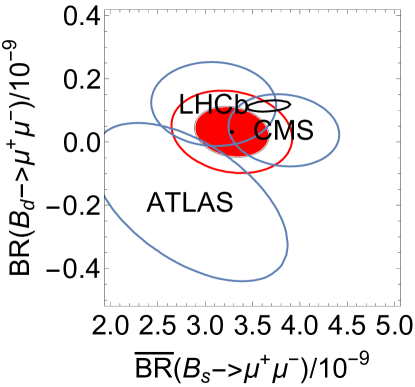
Figure 4: Combination of joint measurements of $\overline{BR}(B_{s}\rightarrow\mu^{+}\mu^{-})$ and $BR(B_{d}\rightarrow\mu^{+}\mu^{-})$. The blue ellipses show the 68$\%$ CL ellipse from each individual experiment (labelled in the centre of each ellipse, respectively), whereas the filled red ellipse shows their combination. The empty red ellipse shows the 95$\%$ CL contour of the combination. The 68$\%$ CL SM prediction with flavio2.3.3 defaults is shown as the small black ellipse.

The Gaussian approximations to the measurements and our combination of them are depicted in Fig. 4. The combination corresponds to

$$\overline{BR}(B_{s}\rightarrow\mu^{+}\mu^{-}) = (3.28\pm 0.26)\times 10^{-9}\,,$$

$$BR(B\rightarrow\mu^{+}\mu^{-}) = (3.21\pm 5.34)\times 10^{-11}\,,$$ (69)

with a correlation coefficient of $\rho=-0.16$. Following Ref. Altmannshofer:2021qrr again and using default flavio2.3.3 settings, one obtains SM predictions of

$$\overline{BR}(B_{s}\rightarrow\mu^{+}\mu^{-})_{SM} = (3.67\pm 0.15)\times 10^{-9}\,,$$

$$BR(B\rightarrow\mu^{+}\mu^{-})_{SM} = (1.14\pm 0.12)\times 10^{-10}\,,$$ (70)

with a correlation coefficient $\rho=+0.28$. These are jointly displayed in Fig. 4 as a small black ellipse. Taking the experimental uncertainties into account and comparing the SM predictions with the two dimensional experimental likelihood, we obtain a one-dimensional pull of 1.6$\sigma$, if both branching ratios are SM-like. The recent update of the CMS measurement (which analysed significantly more integrated luminosity than it had previously) has reduced this one-dimensional pull from 2.3$\sigma$ Altmannshofer:2021qrr .

4.2 Fit results

We display the best-fit points together with the associated $\chi^{2}$ breakdown and associated $p-$value in Table 5. From the table, we note that both models can provide a reasonable fit to the data with $p-$values greater than .1, in contrast to the SM (see Table 1). We also notice that the improvement of the fit to data over that of the SM is considerable and similar in each case: $\sqrt{\Delta\chi^{2}}={3.6}{}$ for the $S_{3}$ model and $\sqrt{\Delta\chi^{2}}={3.6}{}$ for the $Z^{\prime}$ model. We see that while the December 2022 LHCb reanalysis of $R_{K^{(\ast})}$ has reduced the improvement of each model with respect to the SM (evidenced by a lower $\sqrt{\Delta\chi^{2}}$), the $p-$value, and therefore the actual quality of the fit, has improved. This is because the SM was a poor fit previously and now it fits the ‘LFU’ observables well (see Table 1) and because, previously, the new physics models were not very well equipped to explain some of the LFU data (in particular, $R_{K^{\ast}}$ in the low $Q^{2}$ bin) which showed a larger deviation than expected in each model.

Dec 2022 $R_{K^{(\ast)}}$ LHCb:2022qnv
$S_{3}$ model $\chi^{2}$ $n$ $p$ $s\sqrt{|\Delta\chi^{2}|}$ quarks 247.3 224 .14 3.9 LFU 19.7 23 .66 -1.6 global 267.0 247 .16 3.6	$Z^{\prime}$ model $\chi^{2}$ $n$ $p$ $s\sqrt{|\Delta\chi^{2}|}$ quarks 249.1 224 .12 3.7 LFU 18.2 23 .75 -1.0 global 267.4 247 .16 3.6

Previous $R_{K^{(\ast)}}$ LHCb:2017avl ; LHCb:2019hip ; LHCb:2021trn
$S_{3}$ model $\chi^{2}$ $n$ $p$ $s\sqrt{|\Delta\chi^{2}|}$ quarks 245.7 224 .15 3.7 LFU 22.2 23 .51 4.2 global 267.9 247 .15 5.5	$Z^{\prime}$ model $\chi^{2}$ $n$ $p$ $s\sqrt{|\Delta\chi^{2}|}$ quarks 249.3 224 .12 3.1 LFU 22.8 23 .47 4.1 global 272.1 247 .11 5.1

Table 5: Quality-of-fit at the best-fit points of the $S_{3}$ leptoquark model and the $B_{3}-L_{2}$ $Z^{\prime}$ model at $M_{Z^{\prime}}=M_{S_{3}}=3$ TeV. The first column displays the category of observable. $n$ is the number of measurements in each set. The $\chi^{2}$ values for each best-fit point are also shown and $\Delta\chi^{2}:=\chi^{2}_{SM}-\chi^{2}$ and $s:=\text{sign}(\Delta\chi^{2})$. The (updated-$R_{K^{(\ast)}}$) best-fit parameters for the leptoquark model are $\lambda={1.3}{}$, $\theta_{23}={-0.000467}{}$. For the $Z^{\prime}$ model, they are $g_{Z^{\prime}}={0.239}$, $\theta_{23}={-0.0133}$. Only the combined category includes the two fitting parameter reduction in the number of degrees of freedom when calculating $p$. The results using the $R_{K^{(\ast)}}$ LHCb measurements LHCb:2017avl ; LHCb:2019hip ; LHCb:2021trn prior to December 2022 (but including the $BR(B_{s}\rightarrow\mu^{+}\mu^{-})$ update in §4.1) were performed separately and have different best-fit parameter values to these.

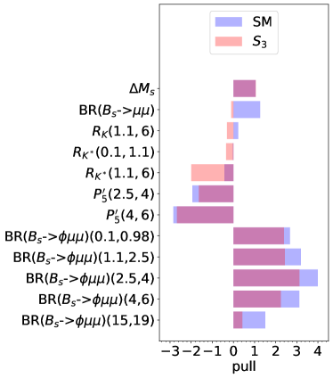
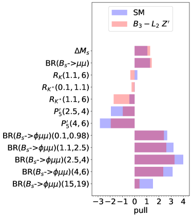
Figure 5: Pulls of some observables of interest for best-fit points of the $S_{3}$ leptoquark model at $M_{S_{3}}=3$ TeV and the ${B_{3}-L_{2}}$ $Z^{\prime}$ model best-fit point at $M_{Z^{\prime}}=3$ TeV. The pull is defined in (71). Numbers in parenthesis denote the domain of the di-lepton invariant mass-squared bin, in GeV². The best-fit parameters for the leptoquark model are $\lambda={1.3}{}$, $\theta_{23}={-0.000467}{}$. For the $Z^{\prime}$ model, they are $g_{Z^{\prime}}={0.239}$, $\theta_{23}={-0.0133}$.

We pick out some $b\rightarrow s\mu^{+}\mu^{-}$ anomaly observables of interest in Fig. 5 to display the pull $P_{i}$ of observable $i$, defined as

$$P_{i}=\frac{T_{i}-E_{i}}{S_{i}}$$ (71)

where $T_{i}$ is the theory prediction, $E_{i}$ is the experimental central value and $S_{i}$ is the experimental uncertainty added to the theoretical uncertainty in quadrature, neglecting correlations with other observables. From the figure, we notice that $P_{\Delta M_{s}}$, i.e. the pull associated with $B_{s}-\overline{B_{s}}$ mixing, is negligibly far from the SM prediction in the $S_{3}$ model best-fit point, as expected since the contributions from the $S_{3}$ are at the one-loop level (as are SM contributions) and furthermore are mass suppressed. While the $Z^{\prime}$ contribution to $\Delta M_{s}$ is mass suppressed, it is at tree-level and therefore enhanced compared to the $S_{3}$ contribution. Even though the $Z^{\prime}$ prediction for $\Delta M_{s}$ does noticeably differ from that of the SM, it is only by a small amount and the effect on quality-of-fit is consequently small. We see from (63) that the new physics contribution to $b\rightarrow s\mu^{+}\mu^{-}$ observables is proportional to $g_{Z^{\prime}}^{2}\sin 2\theta_{23}/M_{Z^{\prime}}^{2}$, whereas the new physics contribution to $\Delta M_{s}$ is proportional to $g_{Z^{\prime}}^{2}\sin^{2}2\theta_{23}/M_{Z^{\prime}}^{2}$, as can be seen from (65), i.e. it involves one additional power of $\sin 2\theta_{23}$. Thus, in the ${B_{3}-L_{2}}$ $Z^{\prime}$ model, decreasing $\theta_{23}$ but increasing $g_{Z^{\prime}}/M_{Z^{\prime}}$ can then provide a reasonable fit both to the $b\rightarrow s\mu^{+}\mu^{-}$ anomalies (which require a sizeable new physics contribution) and to $\Delta M_{s}$, which prefers a small new physics contribution.

We also see that the $\overline{BR}(B_{s}\rightarrow\mu^{+}\mu^{-})$ prediction agrees with the discussion in §4.1, i.e. it is approximately equal to that of the SM in the $Z^{\prime}$ model, whereas it is quite different (and slightly ameliorated) in the $S_{3}$ model. However, the angular distribution $P_{5}^{\prime}$ measurements favour the ${B_{3}-L_{2}}$ $Z^{\prime}$ model in comparison to the $S_{3}$ leptoquark model. Various observables differ in their pulls between the two models, but in the final analysis, when tension in one observable is traded against others, each benchmark model can achieve a similar quality-of-fit, as summarised in Table 5.

4.3 Delineating the preferred parameter space regions

We now delineate the preferred regions of parameter space for each benchmark model, to help facilitate future studies. In Fig. 6, we display a scan over parameter space for each model. The black curves enclose the 95$\%$ CL combined region of parameter space, defined as $\chi^{2}-\chi^{2}_{\text{min}}<5.99$, where $\chi^{2}_{\text{min}}$ is the minimum value of $\chi^{2}$ on the parameter plane. We see in the figure that in the $S_{3}$ model, the preferred region reaches to large values of $-\theta_{23}$ and particular values of $\lambda/M_{S_{3}}$. In fact, the $\chi^{2}$ minimum valley is almost flat. On the other hand, $B_{s}-\overline{B_{s}}$ mixing limits $-\theta_{23}$ to be not too large in the $Z^{\prime}$ model, producing a less degenerate valley in $\chi^{2}$ (note the different scales between the left-hand and right-hand panels’ vertical axis). We note, however, that values $|\theta_{23}|\sim\mathcal{O}(|V_{cb}|)=0.04$ are easily within the good-fit region for each model, meaning that there is no need for any particular flavour alignment. If $\theta_{23}$ were constrained to be much smaller, for example, $V_{cb}$ would be required (speaking from the point of view of the initial gauge eigenbasis) to come dominantly from the up-quark sector. For each model, a very thin region of allowed parameter space extends to the right-hand side of each plot for small values of $-\theta_{23}$ which is not visible (but which can be seen when the ordinate is plotted with a logarithmic scaling, for example).

Figure 6: Two parameter fit to the $S_{3}$ leptoquark model (left panel) and the ${B_{3}-L_{2}}$ $Z^{\prime}$ model (right panel). Shaded regions are those preferred by the global fit at the 95$\%$ confidence level (CL). The yellow region displays the domain $|\theta_{23}|\in\{|V_{cb}|/2,\ 2|V_{cb}|\}$ to guide the eye. The region below the green curve in the right-hand plot is incompatible with the $\Delta M_{s}$ measurement considered on its own at the 95$\%$ CL. There is no such domain in the leptoquark case, explaining the lack of a green curve in the left-hand panel. Our datasets are identical (save for $\overline{BR}(B_{s}\rightarrow\mu^{+}\mu^{-})$ as detailed in §4.1 and $R_{K^{(\ast)}}$) to those defined by smelli2.3.2 and we refer the curious reader to its manual Aebischer:2018iyb , where the observables are enumerated. The fits have been performed with $M_{S_{3}}=3$ TeV and $M_{Z^{\prime}}=3$ TeV, respectively; however each fit is approximately independent of the precise value of the new particle mass (see text). In the right-hand panel, the region to the right-hand side of each vertical dashed magenta contour is excluded for $M_{Z^{\prime}}$/TeV values below $x$ (where $x$ is the labelled value), to 95$\%$ CL Azatov:2022itm .

4.4 High-energy constraints from the LHC

We remind readers of the $M_{S_{3}}>1.4$ TeV bound resulting from an ATLAS di-leptoquark search ATLAS:2020dsk . Given that the leptoquark is coloured, its pair-production proceeds dominantly by QCD production and so this bound is insensitive to the coupling $\lambda$ to SM fermions. There are also high transverse momentum LHC constraints on our scalar leptoquark model coming from e.g. the Drell–Yan process $pp\to\mu^{+}\mu^{-}$, which receives a new physics correction due to the $S_{3}$ leptoquark being exchanged in the $t$-channel. These Drell–Yan constraints, unlike the di-leptoquark search, do not scale only with the leptoquark mass but also scale with the size of its coupling $\lambda$ to quark-lepton pairs, and so they provide complementary information. Using the HighPT package Allwicher:2022gkm ; Allwicher:2022mcg , we computed the $\chi$-squared statistic as a function of the leptoquark model parameters $(\lambda,\theta_{23})$ using the CMS di-muon search CMS:2021ctt implemented within, for a benchmark leptoquark mass of $M_{S_{3}}=3$ TeV (a value which satisfies the di-leptoquark production bound mentioned above). For this mass, we find the 95$\%$ CL limit from $pp\to\mu^{+}\mu^{-}$ to be weak, essentially giving no further constraint on the best-fit region to flavour data that we plot in Fig. 6 (left panel). Specifically, for the domain of $\theta_{23}$ values shown in that plot, the model is consistent with $pp\to\mu^{+}\mu^{-}$ for $\lambda<1.3$ or so ($\lambda=1.3$ is further to the right of the plotted region).

For the $Z^{\prime}$ model the present LHC constraints are also relevant. Fig. 6 displays 95$\%$ CL lower limits upon $M_{Z^{\prime}}$ from CMS measurements of the di-muon mass spectrum CMS:2021ctt . The values of $g_{Z^{\prime}}/M_{Z^{\prime}}$ have been read off from a re-casting of these measurements Azatov:2022itm , neglecting the dependence of the collider bounds upon $\theta_{23}$. This is a good approximation because the dominant LHC signal process is $b\bar{b}\rightarrow Z^{\prime}\rightarrow\mu^{+}\mu^{-}$, whose amplitude is proportional to $\cos^{2}\theta_{23}\approx 1-\theta_{23}^{2}$ and $-\theta_{23}<0.18$ in the well-fit region.

4.5 Upper limits on the $Z^{\prime}$ and $S_{3}$ masses

Fig. 6 shows that $\lambda\times 3\mathrm{~{}TeV}/M_{S_{3}}>0.03$ in the 95$\%$ CL region in the $S_{3}$ leptoquark model, which can be written $M_{S_{3}}/\text{TeV}<100\lambda$. We then find an upper bound on $\lambda$ by considering the width-to-mass ratio of the $S_{3}$, which is $\Gamma_{S_{3}}/M_{S_{3}}=\lambda^{2}/(8\pi)$ Plehn:1997az ; Dorsner:2016wpm . Requiring that the $S_{3}$ is perturbatively coupled, this width-to-mass ratio should not be too large. Requiring $\Gamma_{S_{3}}/M_{S_{3}}<1/3$ for perturbativity, we obtain $\lambda<2.9$. Substituting this in, we find $M_{S_{3}}<~{}290\mathrm{~{}TeV}$, from the combination of the fit to flavour data and perturbativity. This is higher than previous estimates in Refs. Allanach:2020kss ; Azatov:2022itm due in part to the LHCb December 2022 reanalysis of $R_{K^{(\ast)}}$, which made the minimum value on the abscissa smaller. The bound is also subject to large fluctuations from the implementation of the $B_{s}-\overline{B_{s}}$ mixing bound due to different lattice inputs for the SM prediction. Since the LHC di-leptoquark searches only constrain $M_{3}>1.4$ TeV, we see that there is plenty of viable parameter space for a perturbatively coupled $S_{3}$ that explains the $b\rightarrow s\mu^{+}\mu^{-}$ anomalies. The perturbativity and di-leptoquark searches bound combine to imply that $\lambda\times 3\text{~{}TeV}/M_{Z^{\prime}}\leq 6.2$ in the $S_{3}$ model.

Using a similar argument for the $Z^{\prime}$, we can first infer from Fig. 6 that the 95% CL region requires $g_{Z^{\prime}}\times 3\mathrm{~{}TeV}/M_{Z^{\prime}}>0.03$. The width of the $B_{3}-L_{2}$ $Z^{\prime}$ is approximately $\Gamma_{Z^{\prime}}/M_{Z^{\prime}}=13g_{Z^{\prime}}^{2}/(8\pi)$ Allanach:2020kss . Taking $\Gamma_{Z^{\prime}}/M_{Z^{\prime}}<1/3$, we find $g_{Z^{\prime}}<0.80$, implying the following upper bound on the $Z^{\prime}$ mass coming from perturbativity and the global fit: $M_{Z^{\prime}}<~{}80\mathrm{~{}TeV}$, higher than previous estimates in Refs. Allanach:2020kss ; Azatov:2022itm . Given that the LHC constraints only exclude $M_{Z^{\prime}}$ up to about 4.3 TeV, as indicated by the vertical purple dashed lines on the right-hand plot of Fig. 6, we see that there is plenty of viable parameter space for a perturbatively coupled $B_{3}-L_{2}$ $Z^{\prime}$ that explains the $b\rightarrow s\mu^{+}\mu^{-}$ anomalies. We see from Fig. 6 and Ref. Azatov:2022itm , that in the region of 95$\%$ CL fit to flavour data, $M_{Z^{\prime}}\geq 2.0$ TeV. Combining this and perturbativity, we find that $g_{Z^{\prime}}\times 3\text{~{}TeV}/M_{Z^{\prime}}\leq 1.2$ in the $Z^{\prime}$ model.

5 Summary

We have contrasted two bottom-up beyond the SM physics models that can significantly ameliorate the $b\rightarrow s\mu^{+}\mu^{-}$ anomalies in global fits. Since one is a leptoquark model and one a $Z^{\prime}$ model, a naive expectation is that the $Z^{\prime}$ model is disfavoured by the fact that measurements of $B_{s}-{\overline{B}_{s}}$ mixing are broadly compatible with the SM. We have shown that, contrary to the naive expectation, the $B_{s}-{\overline{B}_{s}}$ mixing prediction of the best-fit point of each model is similar, being close to the SM prediction; $\Delta M_{s}$ is therefore not a key discriminator. That said, as Fig. 6 shows, the $B_{s}-\overline{B_{s}}$ mixing constraint limits the $B_{3}-L_{2}$ model’s value of $\theta_{23}$ in the $Z^{\prime}$ model, albeit within a natural range of values that comfortably includes $\theta_{23}\approx|V_{cb}|$, whereas no such preference is strongly evident for the $S_{3}$ model. The $Z^{\prime}$ model that we picked differs in other ways to the leptoquark model in that it couples to di-muons through a vector-like coupling, whereas the leptoquark couples through a purely left-handed coupling. This shifts the predictions for some of the other flavour observables around but in the end the fits are of a similar quality to each other; the improvement in quality-of-fit with respect to the SM of $\sqrt{\Delta\chi^{2}}={3.6}{},{3.6}{}$ in the $S_{3}$ model and in the $Z^{\prime}$ model, respectively.

The LHCb December 2022 reanalysis of $R_{K^{(\ast)}}$ pushes the fits to smaller new physics couplings to fermions for a given $b_{L}-s_{L}$ mixing angle. One unexpected consequence of including the reanalysed measurements was that the fit to each new physics model improves, as Table 5 displays. The improvement with respect to the SM decreases as expected, however each new physics model (with two fitted parameters) still improves upon the SM $\chi^{2}$ by some 12 units. This realisation should be tempered with the risk that the remaining discrepant $b\rightarrow s\mu^{+}\mu^{-}$ observables could potentially receive unaccounted-for long-distance contributions from charm penguins. In Ref. Ciuchini:2022wbq , for example, the discrepancy with SM predictions is ascribed completely to such contributions and is used to parameterise them.

As previously mentioned, both in the ${B_{3}-L_{2}}$ $Z^{\prime}$ model and in the $S_{3}$ leptoquark model, $B-$physics fits are insensitive to scaling the coupling and the mass by the same factor. However, direct searches for the new hypothesised particles do not exhibit this scaling symmetry. The $S_{3}$ model di-leptoquark search constraints only depend sensitively on the mass of the leptoquark Allanach:2019zfr , since the production is governed by QCD and thus via the strong coupling constant, which is of course known from experimental measurement. Single leptoquark production in the $S_{3}$ model does depend sensitively both upon the mass of the leptoquark and upon its coupling Allanach:2017bta . Direct $B_{3}-L_{2}$ $Z^{\prime}$ search constraints also depend upon the coupling and the $Z^{\prime}$ mass Allanach:2020kss . However, the scaling symmetry of the fits allows us in §4.3 to present complete fit constraints upon the three parameters of each model in a two-dimensional plane. We hope that this will facilitate future direct searches for either explanation of the $b\rightarrow s\mu^{+}\mu^{-}$ anomalies.

References

- (1) LHCb Collaboration, R. Aaij et. al., Test of lepton universality with decays, JHEP 08 (2017) 055 [1705.05802].
- (2) LHCb Collaboration, R. Aaij et. al., Search for lepton-universality violation in decays, Phys. Rev. Lett. 122 (2019), no. 19 191801 [1903.09252].
- (3) LHCb Collaboration, R. Aaij et. al., Test of lepton universality in beauty-quark decays, Nature Phys. 18 (2022), no. 3 277–282 [2103.11769].
- (4) LHCb Collaboration, R. Aaij et. al., Tests of lepton universality using and decays, Phys. Rev. Lett. 128 (2022), no. 19 191802 [2110.09501].
- (5) CMS Collaboration, Measurement of decay properties and search for the decay in proton-proton collisions at , .
- (6) J. Aebischer, J. Kumar, P. Stangl and D. M. Straub, A Global Likelihood for Precision Constraints and Flavour Anomalies, Eur. Phys. J. C 79 (2019), no. 6 509 [1810.07698].
- (7) LHCb Collaboration, Test of lepton universality in decays, 2212.09152.
- (8) R. Alonso, B. Grinstein and J. Martin Camalich, gauge invariance and the shape of new physics in rare decays, Phys. Rev. Lett. 113 (2014) 241802 [1407.7044].
- (9) ATLAS Collaboration, M. Aaboud et. al., Study of the rare decays of and mesons into muon pairs using data collected during 2015 and 2016 with the ATLAS detector, JHEP 04 (2019) 098 [1812.03017].
- (10) LHCb Collaboration, R. Aaij et. al., Measurement of the branching fraction and effective lifetime and search for decays, Phys. Rev. Lett. 118 (2017), no. 19 191801 [1703.05747].
- (11) LHCb Collaboration, R. Aaij et. al., Differential branching fractions and isospin asymmetries of decays, JHEP 06 (2014) 133 [1403.8044].
- (12) HPQCD Collaboration, W. G. Parrott, C. Bouchard and C. T. H. Davies, and form factors from fully relativistic lattice QCD, 2207.12468.
- (13) LHCb Collaboration, R. Aaij et. al., Angular analysis and differential branching fraction of the decay , JHEP 09 (2015) 179 [1506.08777].
- (14) CDF Collaboration, Precise Measurements of Exclusive Decay Amplitudes Using the Full CDF Data Set, .
- (15) LHCb Collaboration, R. Aaij et. al., Measurement of Form-Factor-Independent Observables in the Decay , Phys. Rev. Lett. 111 (2013) 191801 [1308.1707].
- (16) LHCb Collaboration, R. Aaij et. al., Angular analysis of the decay using 3 fb-1 of integrated luminosity, JHEP 02 (2016) 104 [1512.04442].
- (17) ATLAS Collaboration, M. Aaboud et. al., Angular analysis of decays in collisions at TeV with the ATLAS detector, JHEP 10 (2018) 047 [1805.04000].
- (18) CMS Collaboration, A. M. Sirunyan et. al., Measurement of angular parameters from the decay in proton-proton collisions at 8 TeV, Phys. Lett. B 781 (2018) 517–541 [1710.02846].
- (19) CMS Collaboration, V. Khachatryan et. al., Angular analysis of the decay from pp collisions at TeV, Phys. Lett. B 753 (2016) 424–448 [1507.08126].
- (20) C. Bobeth, M. Chrzaszcz, D. van Dyk and J. Virto, Long-distance effects in from analyticity, Eur. Phys. J. C 78 (2018), no. 6 451 [1707.07305].
- (21) N. Gubernari, M. Reboud, D. van Dyk and J. Virto, Improved theory predictions and global analysis of exclusive processes, JHEP 09 (2022) 133 [2206.03797].
- (22) A. J. Buras and E. Venturini, The exclusive vision of rare K and B decays and of the quark mixing in the standard model, Eur. Phys. J. C 82 (2022), no. 7 615 [2203.11960].
- (23) A. J. Buras, Standard Model Predictions for Rare K and B Decays without New Physics Infection, 2209.03968.
- (24) G. Isidori, D. Lancierini, P. Owen and N. Serra, On the significance of new physics in b→s+ decays, Phys. Lett. B 822 (2021) 136644 [2104.05631].
- (25) M. Algueró, B. Capdevila, S. Descotes-Genon, J. Matias and M. Novoa-Brunet, global fits after and , Eur. Phys. J. C 82 (2022), no. 4 326 [2104.08921].
- (26) W. Altmannshofer and P. Stangl, New physics in rare B decays after Moriond 2021, Eur. Phys. J. C 81 (2021), no. 10 952 [2103.13370].
- (27) M. Ciuchini, M. Fedele, E. Franco, A. Paul, L. Silvestrini and M. Valli, Lessons from the angular analyses, Phys. Rev. D 103 (2021), no. 1 015030 [2011.01212].
- (28) T. Hurth, F. Mahmoudi, D. M. Santos and S. Neshatpour, More Indications for Lepton Nonuniversality in , Phys. Lett. B 824 (2022) 136838 [2104.10058].
- (29) A. Greljo, J. Salko, A. Smolkovič and P. Stangl, Rare decays meet high-mass Drell-Yan, 2212.10497.
- (30) U. Egede, S. Nishida, M. Patel and M.-H. Schune, Electroweak Penguin Decays of -Flavoured Hadrons, 2205.05222.
- (31) B. C. Allanach, explanation of the neutral current anomalies, Eur. Phys. J. C 81 (2021), no. 1 56 [2009.02197]. [Erratum: Eur.Phys.J.C 81, 321 (2021)].
- (32) G. Hiller and I. Nisandzic, and beyond the standard model, Phys. Rev. D 96 (2017), no. 3 035003 [1704.05444].
- (33) A. Angelescu, D. Bečirević, D. A. Faroughy and O. Sumensari, Closing the window on single leptoquark solutions to the -physics anomalies, JHEP 10 (2018) 183 [1808.08179].
- (34) A. Angelescu, D. Bečirević, D. A. Faroughy, F. Jaffredo and O. Sumensari, Single leptoquark solutions to the B-physics anomalies, Phys. Rev. D 104 (2021), no. 5 055017 [2103.12504].
- (35) B. Gripaios, Composite Leptoquarks at the LHC, JHEP 02 (2010) 045 [0910.1789].
- (36) B. Gripaios, M. Nardecchia and S. A. Renner, Composite leptoquarks and anomalies in -meson decays, JHEP 05 (2015) 006 [1412.1791].
- (37) J. Davighi, M. Kirk and M. Nardecchia, Anomalies and accidental symmetries: charging the scalar leptoquark under Lμ Lτ, JHEP 12 (2020) 111 [2007.15016].
- (38) A. Greljo, P. Stangl and A. E. Thomsen, A model of muon anomalies, Phys. Lett. B 820 (2021) 136554 [2103.13991].
- (39) A. Greljo, Y. Soreq, P. Stangl, A. E. Thomsen and J. Zupan, Muonic force behind flavor anomalies, JHEP 04 (2022) 151 [2107.07518].
- (40) J. Davighi, A. Greljo and A. E. Thomsen, Leptoquarks with Exactly Stable Protons, 2202.05275.
- (41) I. de Medeiros Varzielas and G. Hiller, Clues for flavor from rare lepton and quark decays, JHEP 06 (2015) 072 [1503.01084].
- (42) J. Heeck and A. Thapa, Explaining lepton-flavor non-universality and self-interacting dark matter with , Eur. Phys. J. C 82 (2022), no. 5 480 [2202.08854].
- (43) L. Di Luzio, A. Greljo and M. Nardecchia, Gauge leptoquark as the origin of B-physics anomalies, Phys. Rev. D 96 (2017), no. 11 115011 [1708.08450].
- (44) L. Di Luzio, J. Fuentes-Martin, A. Greljo, M. Nardecchia and S. Renner, Maximal Flavour Violation: a Cabibbo mechanism for leptoquarks, JHEP 11 (2018) 081 [1808.00942].
- (45) A. Greljo and B. A. Stefanek, Third family quark–lepton unification at the TeV scale, Phys. Lett. B 782 (2018) 131–138 [1802.04274].
- (46) W. Altmannshofer, S. Gori, M. Pospelov and I. Yavin, Quark flavor transitions in models, Phys. Rev. D 89 (2014) 095033 [1403.1269].
- (47) A. Crivellin, G. D’Ambrosio and J. Heeck, Explaining , and in a two-Higgs-doublet model with gauged , Phys. Rev. Lett. 114 (2015) 151801 [1501.00993].
- (48) A. Crivellin, G. D’Ambrosio and J. Heeck, Addressing the LHC flavor anomalies with horizontal gauge symmetries, Phys. Rev. D 91 (2015), no. 7 075006 [1503.03477].
- (49) A. Crivellin, L. Hofer, J. Matias, U. Nierste, S. Pokorski and J. Rosiek, Lepton-flavour violating decays in generic models, Phys. Rev. D 92 (2015), no. 5 054013 [1504.07928].
- (50) W. Altmannshofer and I. Yavin, Predictions for lepton flavor universality violation in rare B decays in models with gauged , Phys. Rev. D 92 (2015), no. 7 075022 [1508.07009].
- (51) R. Alonso, P. Cox, C. Han and T. T. Yanagida, Flavoured local symmetry and anomalous rare decays, Phys. Lett. B 774 (2017) 643–648 [1705.03858].
- (52) C. Bonilla, T. Modak, R. Srivastava and J. W. F. Valle, gauge symmetry as a simple description of anomalies, Phys. Rev. D 98 (2018), no. 9 095002 [1705.00915].
- (53) B. C. Allanach and J. Davighi, Third family hypercharge model for and aspects of the fermion mass problem, JHEP 12 (2018) 075 [1809.01158].
- (54) J. Davighi, Connecting neutral current anomalies with the heaviness of the third family, in 54th Rencontres de Moriond on QCD and High Energy Interactions, pp. 91–94, ARISF, 5, 2019. 1905.06073.
- (55) B. C. Allanach and J. Davighi, Naturalising the third family hypercharge model for neutral current -anomalies, Eur. Phys. J. C 79 (2019), no. 11 908 [1905.10327].
- (56) B. C. Allanach, J. E. Camargo-Molina and J. Davighi, Global fits of third family hypercharge models to neutral current B-anomalies and electroweak precision observables, Eur. Phys. J. C 81 (2021), no. 8 721 [2103.12056].
- (57) D. Aristizabal Sierra, F. Staub and A. Vicente, Shedding light on the anomalies with a dark sector, Phys. Rev. D 92 (2015), no. 1 015001 [1503.06077].
- (58) A. Celis, J. Fuentes-Martin, M. Jung and H. Serodio, Family nonuniversal Z’ models with protected flavor-changing interactions, Phys. Rev. D 92 (2015), no. 1 015007 [1505.03079].
- (59) A. Greljo, G. Isidori and D. Marzocca, On the breaking of Lepton Flavor Universality in B decays, JHEP 07 (2015) 142 [1506.01705].
- (60) A. Falkowski, M. Nardecchia and R. Ziegler, Lepton Flavor Non-Universality in B-meson Decays from a U(2) Flavor Model, JHEP 11 (2015) 173 [1509.01249].
- (61) C.-W. Chiang, X.-G. He and G. Valencia, Z’ model for b→s flavor anomalies, Phys. Rev. D 93 (2016), no. 7 074003 [1601.07328].
- (62) S. M. Boucenna, A. Celis, J. Fuentes-Martin, A. Vicente and J. Virto, Non-abelian gauge extensions for B-decay anomalies, Phys. Lett. B 760 (2016) 214–219 [1604.03088].
- (63) S. M. Boucenna, A. Celis, J. Fuentes-Martin, A. Vicente and J. Virto, Phenomenology of an model with lepton-flavour non-universality, JHEP 12 (2016) 059 [1608.01349].
- (64) P. Ko, Y. Omura, Y. Shigekami and C. Yu, LHCb anomaly and B physics in flavored Z’ models with flavored Higgs doublets, Phys. Rev. D 95 (2017), no. 11 115040 [1702.08666].
- (65) R. Alonso, P. Cox, C. Han and T. T. Yanagida, Anomaly-free local horizontal symmetry and anomaly-full rare B-decays, Phys. Rev. D 96 (2017), no. 7 071701 [1704.08158].
- (66) Y. Tang and Y.-L. Wu, Flavor non-universal gauge interactions and anomalies in B-meson decays, Chin. Phys. C 42 (2018), no. 3 033104 [1705.05643]. [Erratum: Chin.Phys.C 44, 069101 (2020)].
- (67) D. Bhatia, S. Chakraborty and A. Dighe, Neutrino mixing and anomaly in U(1)X models: a bottom-up approach, JHEP 03 (2017) 117 [1701.05825].
- (68) K. Fuyuto, H.-L. Li and J.-H. Yu, Implications of hidden gauged model for anomalies, Phys. Rev. D 97 (2018), no. 11 115003 [1712.06736].
- (69) L. Bian, H. M. Lee and C. B. Park, -meson anomalies and Higgs physics in flavored model, Eur. Phys. J. C 78 (2018), no. 4 306 [1711.08930].
- (70) S. F. King, and the origin of Yukawa couplings, JHEP 09 (2018) 069 [1806.06780].
- (71) G. H. Duan, X. Fan, M. Frank, C. Han and J. M. Yang, A minimal extension of MSSM in light of the B decay anomaly, Phys. Lett. B 789 (2019) 54–58 [1808.04116].
- (72) Z. Kang and Y. Shigekami, versus flavor changing neutral current induced by the light boson, JHEP 11 (2019) 049 [1905.11018].
- (73) L. Calibbi, A. Crivellin, F. Kirk, C. A. Manzari and L. Vernazza, models with less-minimal flavour violation, Phys. Rev. D 101 (2020), no. 9 095003 [1910.00014].
- (74) W. Altmannshofer, J. Davighi and M. Nardecchia, Gauging the accidental symmetries of the standard model, and implications for the flavor anomalies, Phys. Rev. D 101 (2020), no. 1 015004 [1909.02021].
- (75) B. Capdevila, A. Crivellin, C. A. Manzari and M. Montull, Explaining and the Cabibbo angle anomaly with a vector triplet, Phys. Rev. D 103 (2021), no. 1 015032 [2005.13542].
- (76) J. Davighi, Anomalous Z’ bosons for anomalous B decays, JHEP 08 (2021) 101 [2105.06918].
- (77) B. Allanach and J. Davighi, helps select models for anomalies, 2205.12252.
- (78) D. King, A. Lenz and T. Rauh, Bs mixing observables and —Vtd/Vts— from sum rules, JHEP 05 (2019) 034 [1904.00940].
- (79) B. Allanach, F. S. Queiroz, A. Strumia and S. Sun, models for the LHCb and muon anomalies, Phys. Rev. D 93 (2016), no. 5 055045 [1511.07447]. [Erratum: Phys.Rev.D 95, 119902 (2017)].
- (80) B. C. Allanach, J. M. Butterworth and T. Corbett, Large hadron collider constraints on some simple models for anomalies, Eur. Phys. J. C 81 (2021), no. 12 1126 [2110.13518].
- (81) A. Azatov, F. Garosi, A. Greljo, D. Marzocca, J. Salko and S. Trifinopoulos, New physics in b → s: FCC-hh or a muon collider?, JHEP 10 (2022) 149 [2205.13552].
- (82) B. C. Allanach, B. Gripaios and T. You, The case for future hadron colliders from decays, JHEP 03 (2018) 021 [1710.06363].
- (83) B. C. Allanach, T. Corbett and M. Madigan, Sensitivity of Future Hadron Colliders to Leptoquark Pair Production in the Di-Muon Di-Jets Channel, Eur. Phys. J. C 80 (2020), no. 2 170 [1911.04455].
- (84) V. Gherardi, D. Marzocca and E. Venturini, Low-energy phenomenology of scalar leptoquarks at one-loop accuracy, JHEP 01 (2021) 138 [2008.09548].
- (85) Particle Data Group Collaboration, P. A. Zyla et. al., Review of Particle Physics, PTEP 2020 (2020), no. 8 083C01.
- (86) B. C. Allanach, J. Davighi and S. Melville, An Anomaly-free Atlas: charting the space of flavour-dependent gauged extensions of the Standard Model, JHEP 02 (2019) 082 [1812.04602]. [Erratum: JHEP 08, 064 (2019)].
- (87) J. Davighi and J. Tooby-Smith, Flatland: abelian extensions of the Standard Model with semi-simple completions, 2206.11271.
- (88) R. Bause, G. Hiller, T. Höhne, D. F. Litim and T. Steudtner, B-anomalies from flavorful U(1)′ extensions, safely, Eur. Phys. J. C 82 (2022), no. 1 42 [2109.06201].
- (89) A. L. Kagan, G. Perez, T. Volansky and J. Zupan, General Minimal Flavor Violation, Phys. Rev. D 80 (2009) 076002 [0903.1794].
- (90) R. Barbieri, G. Isidori, J. Jones-Perez, P. Lodone and D. M. Straub, and Minimal Flavour Violation in Supersymmetry, Eur. Phys. J. C 71 (2011) 1725 [1105.2296].
- (91) J. Aebischer, W. Altmannshofer, D. Guadagnoli, M. Reboud, P. Stangl and D. M. Straub, -decay discrepancies after Moriond 2019, Eur. Phys. J. C 80 (2020), no. 3 252 [1903.10434].
- (92) V. Gherardi, D. Marzocca and E. Venturini, Matching scalar leptoquarks to the SMEFT at one loop, JHEP 07 (2020) 225 [2003.12525]. [Erratum: JHEP 01, 006 (2021)].
- (93) A. Carmona, A. Lazopoulos, P. Olgoso and J. Santiago, Matchmakereft: automated tree-level and one-loop matching, SciPost Phys. 12 (2022), no. 6 198 [2112.10787].
- (94) J. de Blas, J. C. Criado, M. Perez-Victoria and J. Santiago, Effective description of general extensions of the Standard Model: the complete tree-level dictionary, JHEP 03 (2018) 109 [1711.10391].
- (95) N. Košnik and A. Smolkovič, Lepton flavor universality and violation in an leptoquark model, Phys. Rev. D 104 (2021), no. 11 115004 [2108.11929].
- (96) B. Grzadkowski, M. Iskrzynski, M. Misiak and J. Rosiek, Dimension-Six Terms in the Standard Model Lagrangian, JHEP 10 (2010) 085 [1008.4884].
- (97) J. Aebischer, A. Crivellin, M. Fael and C. Greub, Matching of gauge invariant dimension-six operators for and transitions, JHEP 05 (2016) 037 [1512.02830].
- (98) L. Di Luzio, M. Kirk and A. Lenz, Updated -mixing constraints on new physics models for anomalies, Phys. Rev. D 97 (2018), no. 9 095035 [1712.06572].
- (99) K. De Bruyn, R. Fleischer, R. Knegjens, P. Koppenburg, M. Merk, A. Pellegrino and N. Tuning, Probing New Physics via the Effective Lifetime, Phys. Rev. Lett. 109 (2012) 041801 [1204.1737].
- (100) W. Altmannshofer, C. Niehoff and D. M. Straub, as current and future probe of new physics, JHEP 05 (2017) 076 [1702.05498].
- (101) ATLAS Collaboration, G. Aad et. al., Search for pairs of scalar leptoquarks decaying into quarks and electrons or muons in = 13 TeV collisions with the ATLAS detector, JHEP 10 (2020) 112 [2006.05872].
- (102) LHCb Collaboration, R. Aaij et. al., Analysis of Neutral B-Meson Decays into Two Muons, Phys. Rev. Lett. 128 (2022), no. 4 041801 [2108.09284].
- (103) L. Allwicher, D. A. Faroughy, F. Jaffredo, O. Sumensari and F. Wilsch, Drell-Yan Tails Beyond the Standard Model, 2207.10714.
- (104) L. Allwicher, D. A. Faroughy, F. Jaffredo, O. Sumensari and F. Wilsch, HighPT: A Tool for high- Drell-Yan Tails Beyond the Standard Model, 2207.10756.
- (105) CMS Collaboration, A. M. Sirunyan et. al., Search for resonant and nonresonant new phenomena in high-mass dilepton final states at = 13 TeV, JHEP 07 (2021) 208 [2103.02708].
- (106) T. Plehn, H. Spiesberger, M. Spira and P. M. Zerwas, Formation and decay of scalar leptoquarks / squarks in e p collisions, Z. Phys. C 74 (1997) 611–614 [hep-ph/9703433].
- (107) I. Doršner, S. Fajfer, A. Greljo, J. F. Kamenik and N. Košnik, Physics of leptoquarks in precision experiments and at particle colliders, Phys. Rept. 641 (2016) 1–68 [1603.04993].
- (108) M. Ciuchini, M. Fedele, E. Franco, A. Paul, L. Silvestrini and M. Valli, Constraints on Lepton Universality Violation from Rare Decays, 2212.10516.