GalaxyFlow: Upsampling Hydrodynamical Simulations for Realistic Gaia Mock Catalogs

Abstract

Cosmological $N$-body simulations of galaxies operate at the level of “star particles" with a mass resolution on the scale of thousands of solar masses. Turning these simulations into stellar mock catalogs requires “upsampling" the star particles into individual stars following the same phase-space density. In this paper, we demonstrate that normalizing flows provide a viable upsampling method that greatly improves on conventionally-used kernel smoothing algorithms such as EnBiD. We demonstrate our flow-based upsampling technique, dubbed GalaxyFlow, on a neighborhood of the Solar location in two simulated galaxies: Auriga 6 and h277. By eye, GalaxyFlow produces stellar distributions that are smoother than EnBiD-based methods and more closely match the Gaia DR3 catalog. For a quantitative comparison of generative model performance, we introduce a novel multi-model classifier test. Using this classifier test, we show that GalaxyFlow more accurately estimates the density of the underlying star particles than previous methods.

1 Introduction

Large, detailed astronomical surveys are revolutionizing our understanding of the kinematic, photometric, and spectroscopic properties of the Milky Way and its satellites. Surveys such as SDSS (York et al., 2000), DES (The Dark Energy Survey Collaboration, 2005), and Gaia (Gaia Collaboration et al., 2016, 2018, 2021) have revealed aspects of the Milky Way’s merger history, dark matter substructure, stellar streams, satellite dwarf galaxies, and more. As existing surveys continue and new observatories (e.g., JWST (Gardner, 2009), Vera Rubin Telescope (LSST Dark Energy Science Collaboration, 2012), Grace Roman Space Telescope (Spergel et al., 2015)) join them, our knowledge of the Milky Way’s constituents will continue to grow tremendously.

These massive datasets require equally sophisticated simulations in order to fully understand and interpret the underlying cosmological and astrophysical parameters of the Milky Way. Additionally, accurate simulations provide a proving ground for new analysis methods. In particular, given Gaia’s unique capability to measure proper motions, accurate and realistic simulations of Gaia observations must match the kinematics of the Galaxy’s stars in addition to matching the stars’ spatial distribution.

Broadly speaking, two approaches exist to generate synthetic Milky Way-like galaxies with a level of detail similar to actual Gaia observations. In the first approach, synthetic stars are sampled from an analytic model for the Milky Way. For example, Rybizki et al. (2018) generated a Gaia-like catalog from the Besançon model of Robin et al. (2003) using the Galaxia code (Sharma et al., 2011). Such analytic models can be closely tuned to observed properties of the Galaxy. Although those models are beneficial when working with Gaia data, the underlying model of the Galaxy consists of completely smooth distributions with no substructure, streams, or merger history. For analyses that target these and other non-equilibrium properties of the Milky Way, this type of simulation may not serve all necessary purposes.

In the second approach, synthetic observations are taken of fully cosmological $N$-body simulations of Milky Way-like galaxies. State-of-the-art simulations consider dark matter and baryons with smoothed particle hydrodynamics, generating simulated galaxies that appear very similar to our own in many respects — although, of course, the precise merger history and local environment of the simulated galaxies can differ from those of the Milky Way, which may have important effects on the detailed properties of the stellar kinematics. These simulations have shed light on various interesting anomalies, such as the too-big-to-fail problem (Boylan-Kolchin et al., 2011, 2012; Brooks & Zolotov, 2014; Papastergis et al., 2015), the missing satellite problem (Klypin et al., 1999; Moore et al., 1999; Brooks et al., 2013; Sawala et al., 2013; Sawala et al., 2016; Wetzel et al., 2016a; Despali & Vegetti, 2017; Garrison-Kimmel et al., 2017), and others. Unlike analytic models, $N$-body simulations naturally contain realistic non-equilibrium effects and kinematically-consistent substructure evolved from galaxy mergers.

However, the $N$-body simulations all operate at the level of “star particles": objects with masses generally on the order of $10^{3}-10^{4}\,M_{\odot}$, each of which represents an entire population of stars. As a result, these simulations are not directly suitable for comparison with Milky Way stellar populations from large survey data. To create a realistic Gaia-like survey catalog from these $N$-body simulations, star particles must be spread out in phase space via some “upsampling” technique. The goal of any such technique should be to produce a dataset of upsampled stars that follows the same kinematic phase space distribution as the original star particles, so as to preserve the self-consistent kinematics of the cosmological simulation. In particular, a good upsampling technique should not result in kinematic artifacts or any other artificial substructure at length scales below the simulation resolution (which is ${\mathcal{O}}(10^{2})$ pc for current state-of-the-art $N$-body simulations with baryons); instead it should be “smooth" on scales smaller than the simulation resolution.

Several catalogs which simulate the capabilities of the Gaia telescope have been constructed from $N$-body simulations of dark matter and baryons. Lowing et al. (2015) is an early example, as are the Aurigaia (Grand et al., 2018) and the Ananke (Sanderson et al., 2020) catalogs, derived from the Auriga (Grand et al., 2017) and the Feedback In Realistic Environments (FIRE) Latte simulations (Wetzel et al., 2016b; Hopkins et al., 2018), respectively.

The Ananke and Aurigaia catalogs use the EnBiD algorithm (Sharma & Steinmetz, 2006) to estimate the phase space density of the star particles and spread them out by adaptive kernel smoothing. The EnBiD algorithm first tessellates the position/velocity space into hypercubes, each containing a single star particle, using an entropy-based criterion. A length scale of each hypercube, such as a side length, can be used as a bandwidth for the (Gaussian) kernel smoothing. The upsampling is accomplished by drawing samples from the kernel.

However, kernel smoothing algorithms suffer from the curse of dimensionality; due to the sparsity of the data in high-dimensional space, the EnBiD algorithm generates a stellar distribution that is insufficiently smooth at scales near the kernel bandwidth. This lack of smoothness can be seen in plots in proper motion and Galactocentric velocity (see Figure 1), which reveal a clumpiness to the stars in the simulated Gaia catalogs. These clumps track the original star particles and clearly do not appear in real Gaia observations. Given that the actual Gaia dataset is much smoother than the mock catalogs, improved algorithms for smoothing upsampled stars from the star particles are required to generate high-quality mock catalogs.

In this paper, we demonstrate a dramatically improved synthetic star upsampling technique using state-of-the-art density estimation methods, namely normalizing flows (for recent reviews and original references see e.g. Kobyzev et al. 2021; Papamakarios et al. 2021). A key feature of normalizing flows is their ability to sample from the learned density. A normalizing flow that has learned an accurate phase space density is therefore immediately an efficient upsampling algorithm. We will dub our approach GalaxyFlow.

Normalizing flows have previously been used to accurately estimate the phase space density of stars in a galaxy. Green & Ting (2020) was an early study demonstrating the idea in a Plummer sphere. An et al. (2021); Naik et al. (2022) use a mock dataset from analytic galaxy models to confirm the idea by using masked autoregressive flows (MAF; Papamakarios et al., 2017), and show the estimated density can be used for recovering the gravitational potential and acceleration. Buckley et al. (2022) applies MAF to estimate the density of stars in an $N$-body simulated galaxy and uses the density estimate to estimate the local gravitational acceleration and mass density. MAFs are used in Shih et al. (2022) as part of a model-agnostic “anomaly detector” to identify stellar streams in Gaia data. These successes of flows in accurately estimating stellar phase space densities in both simulated and actual astronomical datasets give us confidence that they should be effective upsamplers of galaxy simulations.

In this work, instead of using a MAF, we will use another type of normalizing flow: continuous normalizing flows (CNF; Chen et al., 2018; Grathwohl et al., 2019), which have an excellent inductive bias for modeling smooth distributions. CNFs have been shown to be effective in recovering the densities of various analytic models (Green et al., 2022). This theoretical and empirical evidence indicates that a CNF can be a good flow model for reducing the clumpiness of the upsampled dataset. In Appendix A, we will explicitly show that a CNF performs better than a MAF by our upsampling evaluation metrics.

GalaxyFlow is a physics model-independent upsampling technique as it relies only on the density estimation through a CNF; the upsampling can be applied to a wide range of $N$-body simulations. As a concrete demonstration of our upsampling method, we use the star particles in a simulated galaxy called Auriga 6 (Grand et al., 2017) – the underlying $N$-body simulation used for building the Aurigaia catalog. We will compare the GalaxyFlow upsampling results to a simplified EnBiD algorithm that closely mimics the upsampling algorithm in Aurigaia. Though we use the Auriga 6 simulation for concreteness, nothing about GalaxyFlow depends on the details of this simulation, and it can be applied to a wide range of $N$-body simulations; in Appendix C, we show the results applied to the h277 galaxy simulation generated by the $N$-Body Shop (Zolotov et al., 2012; Loebman et al., 2012).

As this paper aims to be a proof-of-concept demonstration of GalaxyFlow, we will concentrate on the subset of stars in a spherical region within a 3.5 kpc radius of the Sun, as going out to farther radii increases the training time dramatically. Also, limiting ourselves to the Solar neighborhood allows us to make qualitative comparisons to the subset of Gaia DR3 stars that have full 6d positions and velocities. As we will see, considering stars within this window is sufficient for a detailed and definitive demonstration of the efficacy of the GalaxyFlow method.

In a similar vein, our work in this paper concentrates exclusively on the sampling of smooth distributions in position and velocity space. This allows a straightforward upsampling performance comparison between the normalizing flows and EnBiD algorithm.

In future work, we will apply GalaxyFlow to full hydrodynamical simulations, in order to produce complete and realistic Gaia mock catalogs. A full realistic synthetic catalog must also sample stars over a range of masses and metallicities (as well as realistic dust extinction). As we will discuss in our conclusions, these do not present insurmountable problems, but we defer a full algorithm including these effects to future studies.

In addition to showing that the GalaxyFlow-upsampled stellar distributions are smoother by eye, we develop a novel neural network-based multi-model classifier test to determine quantitatively which upsampling method generates a set of synthetic stars closer to the phase-space density of the original star particles. The classifier is trained to distinguish samples from multiple upsamplers, and its output can be utilized for assigning likelihoods to each upsampler given reference dataset, which is not used for training upsamplers. With this multi-model classifier test, we will quantitatively see that GalaxyFlow and EnBiD are nearly perfectly separable, and the reference data is much closer to GalaxyFlow than to EnBiD.

The outline of our paper is as follows. In Section 2, we describe the mock Gaia catalogs and simulations we use in this paper and compare the mock catalogs to the Gaia Data Release 3 (DR3) catalog. In Section 3, we introduce GalaxyFlow and summarize the details of normalizing flows for the upsampling. In Section 4, the simplified EnBiD algorithm used in this paper is explained. In Section 5, we introduce our multi-model classifier test for comparing the performance of upsamplers, and we qualitatively and quantitatively compare the upsampled datasets from GalaxyFlow and the EnBiD algorithm for the Auriga 6 simulation. We conclude in Section 6 by discussing the limitations of our current upsampling and outlining future steps toward a full upsampling algorithm. Additionally, in Appendix A, we compare our upsampling results using a CNF with that of a MAF. In Appendix B, we justify our simplified EnBiD-based upsampler by comparing the upsampled dataset to the Aurigaia catalog. In Appendix C, we demonstrate the generality of our method by applying it to a second hydrodynamical simulation, the h277 galaxy.

2 Current status of mock Gaia catalogs

To present the current status of mock Gaia catalogs, in this section, we consider two different mock catalogs of Gaia-like observations of a Milky Way-analogue galaxy: Ananke (Sanderson et al., 2020), based on the FIRE Latte simulations (Wetzel et al., 2016b; Hopkins et al., 2018); and Aurigaia (Grand et al., 2018), derived from the Auriga $N$-body simulations (Grand et al., 2017).

The Latte simulations (Wetzel et al., 2016b; Hopkins et al., 2018), used to generate the Ananke dataset, were produced using the GIZMO code (Hopkins, 2015). The star particle mass in these simulations is initially $7070\,M_{\odot}$. The snapshot has an average particle mass of $5000\,M_{\odot}$, as the star particle masses can shrink over time due to the life cycle of individual stars in the assumed stellar population.

The Auriga suite of simulations was produced using the Arepo magneto-hydrodynamic code (Springel, 2010), from comoving 100 Mpc snapshots of the EAGLE project (Schaye et al., 2015). The characteristic dark matter particle mass is $4\times 10^{4}\,M_{\odot}$, and the baryonic particle mass is $\sim 5000\,M_{\odot}$. Auriga 6, chosen due to its similarity with the Milky Way, has a total mass of $1.01\times 10^{12}\,M_{\odot}$ within the virial radius.

These $N$-body simulations both contain ${\cal O}(10^{7})$ star particles in their Milky Way equivalents. From these particles, the position and velocities of the ${\cal O}(10^{10})$ individual stars needed for a realistic simulation of the Gaia catalog are drawn through an upsampling process. As discussed in the Introduction, both Aurigaia and Ananke used the EnBiD code as the core of their upsampling algorithms. This code estimates the phase-space volume taken up by each massive star particle; this information is then used to spread out the distribution of upsampled stars using a series of probability distributions (chosen to be Gaussian) centered on each star particle in the sampling step (see Section 4 for additional discussion of the EnBiD algorithm). In addition to kinematic information, the upsampling must also account for stellar masses, ages, and metallicity, and observational effects such as dust extinction. In this work, we are primarily concerned with the kinematic sampling and will defer these other important stellar properties for later work.

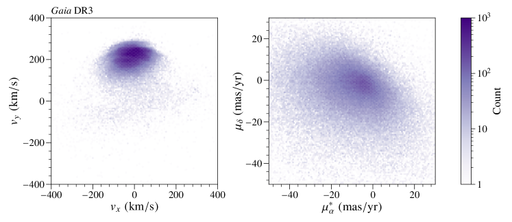
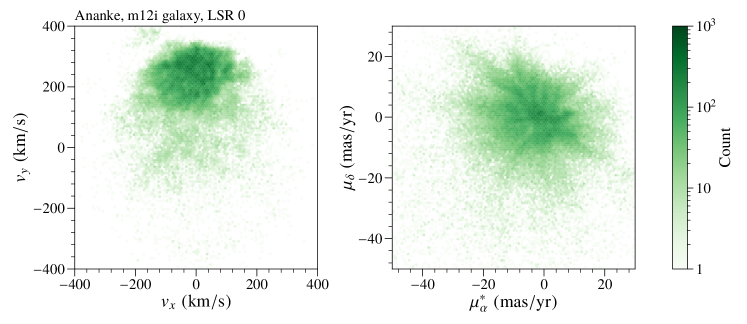
Figure 1: Distributions of Galactocentric velocities $(v_{x},v_{y})$ (left column) and proper motion (right column) for all stars within $15^{\circ}$ of the ICRS coordinate $(\alpha,\delta)=(167.47^{\circ},-4.2^{\circ})$ and with measured radial velocities. We additionally require that the “observed” parallax is more than $3\sigma$ away from $\varpi=0$, in order to remove stars with poorly measured distances. Distributions are shown for real Gaia DR3 data (top row), for Ananke (middle row), and for Aurigaia (bottom row). The Gaia DR3, Ananke, and Aurigaia datasets have 139,164; 94,970; and 2,192,188 stars satisfying the selection criterion, respectively. Note that the Aurigaia catalog presents radial velocities of all the stars so that coverage and sample statistics are quite different from the other datasets.

The kinematic sampling approaches used in Aurigaia and Ananke reproduce many features of the real Gaia data, particularly in the spatial distribution of the upsampled stars. However, especially in velocity space, residual traces of the progenitor star particles remain and can be clearly seen in relatively simple plots of the distribution of stars. As an example, in Figure 1, we show – for all stars with measured position and velocity in a $15^{\circ}$ observational window centered on the ICRS coordinate $(\alpha,\delta)=(167.47^{\circ},-4.2^{\circ})$ – the distribution of proper motions on the sky as well as stellar velocities in Galactocentric coordinates. The center of the $15^{\circ}$ window was chosen to be off of the Galactic disk but is otherwise randomly selected. These distributions are shown for real Gaia DR3 data (Gaia Collaboration et al., 2021) as well as the Ananke and Aurigaia simulations.

The upsampled stars exhibit clustering and streaking in the velocity and proper motion that are not present in the actual Milky Way population as seen by Gaia. We verify in Appendix B that the visually-apparent clusters of simulated stars in proper motion- and velocity-space correspond to individual parent star particles in the original $N$-body simulation.

Note that the three datasets have very different numbers of stars in the same angular patch on the sky (139,164; 94,970; and 2,192,188 stars for Gaia, Ananke, and Aurigaia, respectively). The order-of-magnitude difference in statistics between the mock catalogs is mainly because the Aurigaia catalog provides radial velocities of all the stars (Grand et al., 2018), while the Ananke catalog provides the information for the stars satisfying the magnitude and temperature limits of Gaia DR2 (Sanderson et al., 2020). A similar order-of-magnitude difference can be seen in the total number of sources in Gaia DR3 (Gaia Collaboration et al., 2022) and the number of sources with radial velocities in Gaia DR2 (Gaia Collaboration et al., 2018). As this work is concerned only with the distribution of the stars in phase space, which can be seen regardless of these factors, we do not correct for them.

Figure 2: Distributions of a subset of Gaia DR3 stars in ICRS coordinates. We select stars within $15^{\circ}$ of $(\alpha,\delta)=(167.47^{\circ},-4.2^{\circ})$ and within $3.5$ kpc of the Sun. We discard stars with poorly measured distances, i.e., the observed parallax must be greater than zero parallax by $3\times$ the parallax measurement error. Plots on the diagonals are the marginal distribution of each component. The other plots are the joint distribution of two components. The Gaia DR3 dataset has 979,185 stars satisfying these criteria. Only a small fraction of stars have measured radial velocity, and so the plots including radial velocity have lower statistics, with 135,105 stars.

To further illustrate the comparative smoothness of Gaia, we show the full phase space distribution in ICRS coordinates for the Gaia DR3 stars in Figure 2. The full sample (not requiring a measured radial velocity) contains 979,185 stars. Only a small fraction of stars have measured radial velocity, so plots of radial velocity are statistically suppressed with only 135,105 stars (all other plots use the full sample of stars). Observational effects are apparent in the distance histogram, which falls after 1 kpc instead of continuing to rise as expected for the underlying distribution of stars. Most notably, we see no significant “blotchiness” in the resulting distributions.

2.1 Benchmark Datasets for Training Upsamplers

Our goal is to generate upsampled stars from $N$-body simulations of Milky Way-like galaxies with stellar kinematics which display less clumping than found in the existing suites of mock Gaia datasets (most notably in velocity-space). To achieve this, we train a normalizing flow neural network on the kinematics of star particles from fully-cosmological $N$-body simulations containing both baryons and dark matter. In the main body of this paper, we focus on the Auriga 6 galaxy (Grand et al., 2017). The details of the simulation which produced Auriga 6 have been described in the previous section. In Appendix C, we work with the h277 galaxy to cross-validate our general GalaxyFlow method with a different mock dataset.

The Galactocentric coordinate system of Auriga 6 is oriented in a way that the galactic disk lies in the $xy$-plane, with the assumed Solar location lying in the $-x$ direction. The $z$ coordinate points out of the disk, oriented so that the local motion of disk stars is in the $+y$ direction.

The star particles within 3.5 kpc of the default Solar location of the Aurigaia catalog, $(-8.0,0,0.02)$ kpc, are selected for training our upsamplers. The number of selected star particles in Auriga 6 is 482,412, with a maximum speed of 858.15 km/s. Although we limit the star particles to be upsampled, this dataset is enough for comparing the upsampling performance of various algorithms. Training upsamplers over a full galaxy will be addressed in future work.

3 GalaxyFlow

3.1 Normalizing Flows

GalaxyFlow is based on a type of generative model called normalizing flows. Normalizing flows are a class of neural network which learn a transformation from a simple base probability distribution to a function representing the unknown probability distribution from which the training data was drawn. A fully trained normalizing flow allows for both density estimation of a dataset as well as sample generation from the approximated density distribution. A summary of the idea is as follows.

Let $\vec{z}$ and $\vec{y}$ be $D$-dimensional random variables with the base distribution and training data distribution, respectively. The standard normal distribution is conventionally used as the base distribution because of its tractability. Normalizing flows will learn a bijective transformation $g$ between $\vec{z}$ and $\vec{y}$:

$$\vec{y}=g(\vec{z}).$$ (1)

Once the network has learned this transformation, it is straightforward to upsample the dataset using normalizing flows: randomly select samples from a multidimensional standard normal distribution and then transform them to synthetic data in the training space using the above formula.

By composing a chain of simple, nonlinear bijective functions $g_{i}$:

$$g=g_{N}\circ g_{N-1}\circ\cdots\circ g_{1}.$$ (2)

one can build a highly expressive family of bijections $g$ that are capable of modeling non-trivial distributions. For computational efficiency, we require that inverse and Jacobian determinants of those simple bijections are easy to compute.

Training normalizing flows are based on maximum likelihood estimation. If the inverse transformation of $g$ and the Jacobian determinant $\left|{d\vec{z}}/{d\vec{y}}\right|$ are easy to compute, the change of variable formula can be used to compute the probability density function of $\vec{y}$:

$$p(\vec{y})=p(\vec{z})\cdot\left|\frac{d\vec{z}}{d\vec{y}}\right|=p(g^{-1}(\vec{y}))\cdot\left|\frac{dg^{-1}(\vec{y})}{d\vec{y}}\right|.$$ (3)

By maximizing $\log p(\vec{y})$ (summed over the training data) with respect to the parameters of $g$, the normalizing flow can be fit to the data and learn the underlying probability density.

In addition, normalizing flows are able to learn conditional probabilities if the transformation $g$ is conditioned. This capability is especially useful in modeling the phase space density $f(\vec{r},\vec{v})$, as the full 6-dimensional density need not be learned all at once. Instead, we borrowed the well-performing setup from our previous work (Buckley et al., 2022) and used two separate flows learning position density $p(\vec{r})$ and velocity density conditioned on position, $p(\vec{v}|\vec{r})$. The phase space density $f(\vec{r},\vec{v})$ is modeled by their product as follows.

$$f(\vec{r},\vec{v})=p(\vec{r})p(\vec{v}|\vec{r}).$$ (4)

Note that we do not need to train $p(\vec{r})$ and $p(\vec{v}|\vec{r})$ simultaneously. We will train $p(\vec{r})$ first and then $p(\vec{v}|\vec{r})$.

3.2 Continuous Normalizing Flows

Within the general class of normalizing flows, we have to choose an optimal implementation for smoothly upsampling star particles. Continuous normalizing flows (CNF; Chen et al., 2018; Grathwohl et al., 2019) are a good candidate with an inductive bias suitable for this problem because the transformation smoothly deforms the base distribution to the target distribution.

More specifically, CNF learns the following infinitesimal transformation,

$$g_{t} : \vec{y}\rightarrow\vec{y}+F(\vec{y},t)\cdot dt,$$ (5)

$$g_{t}^{-1} : \vec{y}\rightarrow\vec{y}-F(\vec{y},t)\cdot dt.$$ (6)

Here, the function $F$ is a neural network representing the derivative ${d\vec{y}}/{dt}$ of the trajectory of transformed variables at a latent time $t$. The full chain of transformations is the integral of this infinitesimal transformation, and it is described by a neural ordinary differential equation (neural ODE; Chen et al., 2018),

$$\frac{d}{dt}\vec{y}(t)=F(\vec{y}(t),t).$$ (7)

Note that if $dt$ is finite, the transformation $g_{t}$ is essentially a residual block at a given time, $\vec{y}\rightarrow\vec{y}+\mathcal{F}(\vec{y})$, where $\mathcal{F}$ is the difference between the inputs and outputs of the transformation. Therefore, the neural ODE is considered as a generalization of residual networks for normalizing flows (Haber et al., 2018; Lu et al., 2018; Haber & Ruthotto, 2017; Ruthotto & Haber, 2020), and the parameter $t$ takes the role of the flow index in the chain.

The Jacobian determinant of the transformation can be obtained by solving the following form of the Fokker-Planck equation with zero diffusion (Chen et al., 2018), describing the time evolution of log probability $\log p(\vec{y}(t);t)$ along the trajectory $\vec{y}(t)$ at time $t$:

$$\frac{d}{dt}\log p(\vec{y}(t);t)=-\mathrm{Tr}\left[\frac{\partial F}{\partial\vec{y}(t)}\right].$$ (8)

The trace computation of this equation is often a bottleneck during the training, so Hutchinson’s trace estimator (Grathwohl et al., 2019) can be used to speed up the training. In our case, the cost of evaluating the trace is manageable since we train CNFs for 3D densities; we explicitly evaluate the trace during the training.

Our CNF is implemented using Torchdyn (Poli et al., ) with backend PyTorch (Paszke et al., 2019). The neural ODEs are solved by the Runge-Kutta method of order 4 for both forward and backward directions. For the backward direction, we could numerically invert the forward calculation for the exact invertibility of the flows (Behrmann et al., 2019; Chen et al., 2019) but use the numerical solver again for fast calculation. We will see that this approximate inverse transform is still good enough to model a good upsampler. We set the distribution at $t=0$ to be the base distribution and that at $t=1$ be the target distribution, and the latent time interval is divided into 20 steps. The derivative function $F$ is modeled by a multilayer perceptron (MLP) consisting of 4 hidden layers with 32 nodes each. GELU activations (Hendrycks & Gimpel, 2016) are used in order to model a smooth transformation. For our conditional CNF for modeling $p(\vec{v}|\vec{r})$, the conditioning variables $\vec{r}$ are provided as extra inputs to $F$.

3.3 Training Normalizing Flows for Upsampling Star Particles

We preprocess the position and velocity of the star particles in order to standardize the inputs and separate the sharp boundaries at the edge of the training volume. The CNFs model a smooth transformation in the latent space, so we preprocess to avoid discontinuities. The position vectors $\vec{r}$ are preprocessed as follows in order to construct normalizing flows on an open ball in Euclidean space (Buckley et al., 2022):

1. Centering and scaling: We scale the positional coordinates to transform the 3.5 kpc radius sphere centered on the Sun into a unit ball by the following linear transformation:

   $$\vec{r}\rightarrow\frac{\vec{r}-\vec{r}_{\sun}}{r_{\mathrm{max}}\cdot c},$$ (9)

   where $r_{\mathrm{max}}$ is the radius of the selection window, $\vec{r}_{\odot}$ is the location of the Sun in the galaxy, and $c=1.000001$ is a small constant to avoid putting stars exactly on the boundary.

2. Radial transformation: We then expand the unit ball to cover Euclidean space, i.e.,

   $$\vec{r}\rightarrow\frac{\vec{r}}{|\vec{r}|}\tanh^{-1}\left|\vec{r}\right|.$$ (10)

   This transformation is designed to have well-defined derivatives at the origin.

3. Standardization: We finally rescale the position coordinates by the width of their distributions:

   $$r_{i}\rightarrow\frac{r_{i}-{\mu}_{r_{i}}}{\sigma_{r_{i}}},\quad i=1,2,3,$$ (11)

   where ${\mu}_{r_{i}}$ and $\sigma_{r_{i}}$ are the mean and standard deviations of $r_{i}$ in the training dataset, respectively.

The velocity distribution does not have a sharp boundary at the edge of the observational sphere, so preprocessing the velocity vectors consists only of standardizing the inputs (Step 3 above).

The normalizing flows are then trained to map the base distribution to the target distribution on the preprocessed data space as follows. The loss function is defined as the negative log-likelihood of the flow evaluated on the data. We use an ADAM optimizer (Kingma & Ba, 2014) with learning rate of $10^{-3}$ to minimize the loss function. We randomly select 20% of the training samples as a validation dataset, which is not included in the training epochs. The remaining training datasets are randomly split into 10 mini-batches for each epoch of training. We stop the training when the validation loss has not improved over 50 epochs. The trained network is further refined by restarting training with a reduced learning rate of $10^{-4}$. We train 10 instances of a normalizing flow initialized with different random number seeds, and we ensemble average to improve the performance further.

We generate position and velocity samples using the normalizing flows as follows.

1. Sample Gaussian random numbers from the base distributions.

2. Use the trained normalizing flows to transform the random numbers into position and velocity vectors in the preprocessed space.

3. Use the preprocessors to transform the vectors in the preprocessed space to the position and velocity vectors.

4. We remove outliers by discarding samples with distances from the Sun larger than 3.5 kpc, or with speeds exceeding the maximum speed of the training sample.

4 EnBiD Density Estimation

We compare the phase space distributions generated by the normalizing flows to the distribution generated using the EnBiD algorithm (Sharma & Steinmetz, 2006; Sharma & Johnston, 2009) — the adaptive kernel density estimation used as a base of the upsampling method for constructing the existing state-of-art Gaia mock catalogs. Note that EnBiD itself only estimates the phase space density of the star particles, it does not sample from that density. The sampling is done by placing a multi-dimensional Gaussian distribution at the location of each star particle. The widths of these Gaussians are then set by the phase space density provided by EnBiD.

Given a set of star particles in phase space, EnBiD first partitions the phase space into disjoint boxes, each containing exactly one particle. Each box represents a volume with a unit probability of finding a particle, $1/N$, where $N$ is the total number of particles. The boxes are constructed using the following entropy-based criterion:

1. Start with a box containing all the star particles.

2. For a given box containing $N_{p}$ star particles, calculate the Shannon entropy along each axis. The entropy is estimated by modeling the probability density as a histogram of $N_{p}$ equal-sized bins.

3. Select the axis with minimum entropy.

4. Divide the box in two by dividing the selected axis at the midpoint of the nearest upper and lower neighbors of the mean value of the corresponding component.

5. Repeat the above splitting until all the boxes contain only one particle.

Dividing the axis with minimum entropy prioritizes splitting along axes with clustered structures. This box splitting rule results in small box volumes in regions of high density. The inverse of a box’s volume can be used as a proxy for the phase space density within that box. Each star particle can then be upsampled by drawing from (Gaussian) kernels with smoothing bandwidths determined by hypercube length scales. Aurigaia and Ananke each implement additional smoothing strategies during upsampling to improve upon this basic strategy. For details on the anisotropic kernel smoothing used by Aurigaia see Lowing et al. (2014) and Grand et al. (2018). The Ananke catalog uses a similar method described in Sanderson et al. (2020).

The Aurigaia mock catalog aims to model the real Gaia data accurately and so must sample stellar populations from isochrones, creating synthetic stars with a range of magnitudes and colors. After this sampling, realistic observational effects must be applied. In this work, we are interested only in the sampling of the kinematic phase space: comparing our new technique using normalizing flows to the existing EnBiD-based approach. For this comparison, the full simulation of synthetic stars (including isochrones and observational effects) is unnecessary, so we omit these steps.

To perform a straightforward comparison of normalizing flows and EnBiD without the observational effects and stellar properties as confounding variables, we generate our own catalog using an approximation of the algorithm used by Aurigaia. For simplicity, we do not use anisotropic kernel smoothing. We instead use the following procedure for upsampling each star particle:

1. Use EnBiD to determine the phase space hyperrectangle containing the star particle.

2. For coordinate axis $i$, define $L_{i}$ as the corresponding hyperrectangle side length.

3. Sample phase space coordinates from a 6D Gaussian centered on the original star particle with dispersion in each phase space direction given by $\sigma_{i}^{2}=\frac{1}{48}(\frac{L_{i}}{2})^{2}$

For comparison with samples generated using our normalizing flows, we again restrict ourselves to star particles within 3.5 kpc of the assumed Solar location. In Appendix B, we show that our simplified algorithm is qualitatively similar to the procedure used by Aurigaia, and produces the same visible clumping of stars around progenitor star particles. We conclude that our simplified algorithm remains a fair representation of kernel density estimation for the purposes of this study.

5 Results

5.1 Qualitative results

As Gaia observations cover the full sky, and studies of Galactic kinematics are concerned with the correlations of stellar velocities with their location in position-space, we compare the results of upsampling the parent star particles in the same observational window as in Figure 1. For Auriga 6, this patch contains 3,015 star particles. We upsample the star particles by a factor of 500 to have statistics comparable to that of the Aurigaia catalog: 2,192,188 stars.

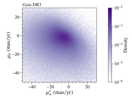
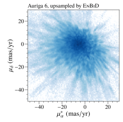
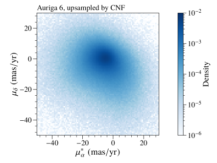
Figure 3: Distributions of proper motion for stars in Gaia DR3 (upper center) and upsampled Auriga 6 stars by EnBiD (lower left) and the CNF (lower right) within $15^{\circ}$ of the ICRS coordinate $(\alpha,\delta)=(167.47^{\circ},-4.2^{\circ})$ with distance from the assumed Solar location within $3.5$ kpc. For Gaia DR3, we additionally require that the “observed” parallax is more than $3\sigma$ away from $\varpi=0$, in order to remove poorly measured stars. After the selection, the Gaia DR3 dataset has 979,185 stars.

In Figure 3, we plot the proper motion for stars upsampled in the patch for the Gaia DR3 catalog and from the Auriga 6 simulations using both EnBiD and the CNF. The phase space sampling using EnBiD results in stars noticeably clumped in proper motion around the parent star particles. These clumps and streaks are similar to the distribution from the Aurigaia catalogs in Figure 1, as both datasets are generated by using the EnBiD algorithm to estimate sampling Gaussian bandwidths. The normalizing flow upsampling gives a smoother proper motion distribution that is closer qualitatively than the EnBiD upsampling to the real Gaia DR3 data while still following the distribution of the parent star particles.

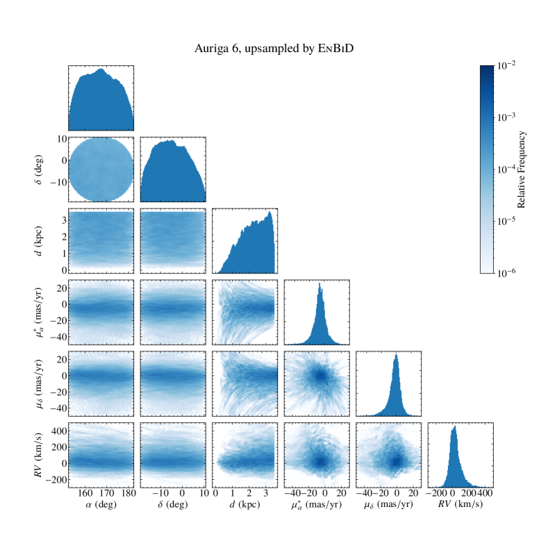
Figure 4: Distributions of EnBiD-upsampled Auriga 6 stars in the ICRS coordinate. We select stars within $15^{\circ}$ from $(\alpha,\delta)=(167.47^{\circ},-4.2^{\circ})$ and with distances from the assumed Solar location less than $3.5$ kpc.

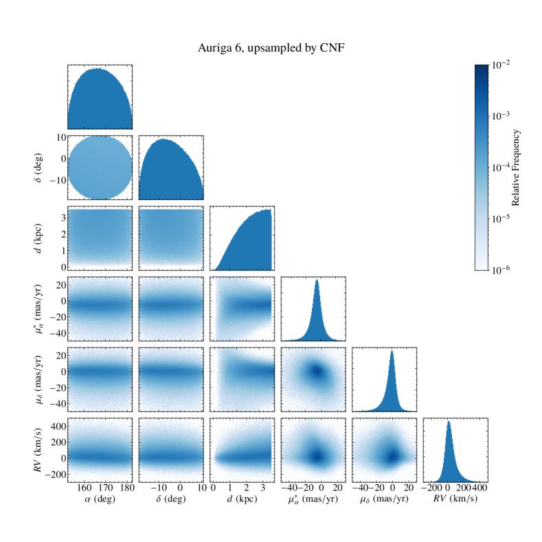
Figure 5: Distributions of CNF-upsampled Auriga 6 stars in the ICRS coordinate. We select stars within $15^{\circ}$ from $(\alpha,\delta)=(167.47^{\circ},-4.2^{\circ})$ and with distance from the assumed Solar location less than $3.5$ kpc.

In Figure 4 and Figure 5, we provide the full six-dimensional phase space (in the ICRS coordinates) of stars upsampled in the patch by EnBiD and the CNF, respectively. We can see the kernel-induced unphysical substructure in each two-dimensional plot in Figure 4, while the CNF distributions in Figure 5 do not have such artifacts. Overall, the blotchiness of EnBiD upsampled star distributions (relative to the density estimate learned by the CNF) indicates that the adaptive kernel density estimation is not the ideal method for star particle upsampling.

5.2 Two-Sample Classifier Metric

While by-eye comparisons of the outputs of CNF are useful, they are necessarily qualitative, as well as limited to one or two dimensions. For a more quantitative, full-phase-space test of the quality of the generative models, we turn to a novel neural classifier test.

The ideal metric to judge the quality of a generative model would be the Neyman-Pearson (NP) optimal binary classifier between reference and generated samples. The classifier output would be monotonic with the likelihood ratio between the reference and generated distributions. If the two follow the same probability distribution (i.e. $p_{\mathrm{ref}}=p_{\mathrm{gen}}$), the NP-optimal classifier would be maximally confused, i.e. the area under the receiver operating characteristic curve (AUC) of the classifier would be 0.5. Conversely, the higher the AUC, the worse the generative model is at modeling the underlying probability distribution of the data.

This “ultimate classifier metric" was recently used by Krause & Shih (2021) in a Large Hadron Collider (LHC) application to demonstrate the fidelity of a fast calorimeter simulation based on masked autoregressive flows trained on GEANT4 reference showers. Using this metric, the authors successfully demonstrate that normalizing flows are better at generating synthetic calorimeter responses than generative adversarial networks. Hence, we may also try this classifier test to determine a better star particle upsampler.

However, this “ultimate classifier metric" has many limitations and drawbacks. Chief among these is that it is only strictly reliable when the classifier is close to optimal. We find this is definitely not the case here because there are simply not enough reference star particles to train a good classifier. In the LHC case, we can always run more GEANT4 simulations to generate more reference data, but here we are limited to the fixed number of star particles in the Auriga simulation. As a result, the classifier training starts to overfit in the very early phase of training, and we end up with AUCs close to 0.5 (0.511 and 0.504 for EnBiD and CNF, respectively). This does not agree with what we found with our qualitative, by-eye comparisons of EnBiD and the reference Auriga simulation data, and indicates the classifier is non-optimal.

Another issue with the “ultimate classifier metric" is that the AUC can be misleading, in the sense that a perfectly suitable generative model could be nevertheless 100% separable from the reference data due to some physically irrelevant “tells" (leading to an AUC of 1). Also, the AUC has rather limited expressiveness as a measure of quality in that it is bounded between 0 and 1. For example, two generative models could both have an AUC of 1, but one could be much better than the other, and it would be impossible to tell using the “ultimate classifier metric".

For these reasons, in the next subsection, we introduce a new classifier-based evaluation score to judge the relative merits of different upsampling generative models, which circumvents these problems with the “ultimate classifier metric".

5.3 Multi-Model Classifier Metric

We dub our new evaluation score the “multi-model classifier metric". This score gives up on judging the absolute quality of a generative model with respect to the reference data, and instead focuses on judging the quality of a generative model relative to a collection of other generative models. In other words, we seek to rank a collection of generative models in terms of which one describes the reference data best.

Given a collection of $N$ generative models, we will first train an $N$-class classifier to distinguish between upsamplings of the same reference data by all the different generative models. Since the training is over upsampled data, we are not limited by training statistics, we are able to learn the difference between these two generative models and verify that they are not equivalent. After this training, we utilize the classifier to assign upsampling performance scores to each upsampler and identify the best upsampler as the one whose probability distribution is closest to the reference dataset. Again, this test cannot tell us the absolute quality of a generative model, but it can tell us which generative model is most similar to the reference data.

We identify the better upsampler by using the average of log-posteriors of each upsampler evaluated on the reference dataset. The log-posterior of a generative model $C$ is defined as follows,

$$\mathrm{LP}(C)=\frac{1}{N_{\mathrm{ref}}}\sum_{i=1}^{N_{\mathrm{ref}}}\log p(C\,|\,\vec{x}^{(i)},\vec{v}^{(i)}),$$ (12)

where $p(C\,|\,\vec{x}^{(i)},\vec{v}^{(i)})$ is the classifier output for model $C$, evaluated on $i$/̄th sample $(\vec{x}^{(i)},\vec{v}^{(i)})$ in the reference dataset.

One advantage of using the log-posterior as our metric is that the difference of posteriors of two upsamplers has a clear probabilistic interpretation. The log-posterior $\mathrm{LP}(C)$ of an upsampler $C$ differs only from the log-likelihood $\mathrm{LL}(C)$ (the log-likelihood that the dataset is drawn from the probability distribution of upsampler $C$) by a constant which is the same when evaluated over both upsamplers:

$$\mathrm{LL}(C) = \frac{1}{N_{\mathrm{ref}}}\sum_{i=1}^{N_{\mathrm{ref}}}\log p(\,\vec{x}^{(i)},\vec{v}^{(i)}\,|\,C),$$ (13)

$$= \mathrm{LP}(C)+\frac{1}{N_{\mathrm{ref}}}\sum_{i=1}^{N_{\mathrm{ref}}}\log\sum_{C^{\prime}}p(\vec{x}^{(i)},\vec{v}^{(i)}\,|\,C^{\prime}).$$ (14)

Note that we train classifiers using a uniform prior of $p(C)=1/N$, and the prior dependence of Eq. (14) is canceled out. Therefore, the difference between the log-posteriors of two different models $C_{1}$ and $C_{2}$ can be considered as the log-likelihood ratio from one upsampler from the other, making these numbers suitable for systematically comparing the performance of upsamplers.

Another advantage of the log-posterior score is that it is not bounded and remains informative even when comparing generative models which may be separable from the reference data. In that case, the AUC becomes uninformative ($\mathrm{AUC}\approx 1$ for both upsamplers), whereas the better model should still be apparent using the log-posterior because our method is based on likelihood ratios for determining the model closer to the reference dataset.

In the rest of this subsection, we will describe our implementation of the multi-model classifier test for $N=2$ models: EnBiD and CNF. In Appendix A, we will show an example of the multi-model classifier test with $N=3$, by including another high-performing upsampler based on the MAF-family of normalizing flows.

For this classifier test, we have to use a large neural network that is robust enough to capture the “clumpy” substructure of the EnBiD upsampled dataset. An under-parameterized network may give incorrect conclusions as such a classifier can smooth out the bumps due to the mean-seeking behavior of the inclusive Kullback-Leibler divergence related to the cross-entropy loss function. We use an MLP consists of four hidden layers with [2048, 1024, 128, 128] nodes each. We use LeakyReLU activations (Maas et al., 2013) in order to avoid dying ReLU problems that may appear when the datasets are too similar.

As the classifier is for testing the generalization performance of the upsamplers, we perform the classifier training and hypothesis testing as follows:

1. Split the selected star particles into training and test datasets for the upsampling. We will use a split ratio of 1:1. Each split contains 241,206 star particles.

2. Train upsamplers using the training dataset of star particles.

3. For each upsampler, generate upsampled datasets with $241,206\times 200$ samples for training the classifiers. Samples outside of the selection window are removed.

4. Train a classifier for comparing the two upsampled datasets.

5. Evaluate the log-posterior on the test star particles to determine the better upsampler.

Half of the upsampled dataset is used as a validation dataset for the classifier. The remaining training datasets are split into 1000 batches for each epoch during the training. The other setup steps for the training are the same as those for training normalizing flows. We stop the training when the validation loss has not improved over 100 epochs.

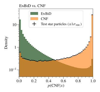
Figure 6: EnBiD (green) vs. CNF (orange) classifier output distributions. Black markers are the classifier output histogram of star particles from the test set, which is not used in training upsamplers. Their vertical error bars are the $1\sigma$ statistical uncertainties.

Table 1: Log-posteriors from the multi-model classifier test for EnBiD vs. CNF. Large (i.e. less negative) log-posterior scores indicate better upsampling performance. We also show the $1\sigma$ statistical uncertainties of the log-posterior scores, which are taken to be the standard error of the mean log-posterior calculated over the finite-sized test dataset.

Classifier:	EnBiD vs. CNF
Upsampler	$\mathrm{LP}(\mathrm{upsampler})$
EnBiD	$-6.222\pm 0.014$
CNF	$-0.344\pm 0.002$

Let us first compare the datasets upsampled by EnBiD and CNF. Recall that the EnBiD-upsampled distribution is clumpy, and the gaps between the Gaussian are visible (as shown in Figure 3). In comparison, the CNF-upsampled dataset has a relatively smooth distribution, and the regions of phase space that would fall between the EnBiD Gaussians are well-populated by the CNF upsampler. As a result, the classifier output distributions of two upsampled datasets are split as in Figure 6. The AUC is 0.952, which is close to 1; the two upsampled datasets are clearly distinguishable, not just by eye, but through the classifier.

Next, we use the classifier to determine which upsampler generates stars whose distribution is closest to that of the original star particles. The test star particles are not close to the EnBiD Gaussians (as these are drawn from a separate training set of star particles) in the 6D phase space; therefore, we expect that the classifier will mostly consider the test star particles as CNF-upsampled stars. The classifier output distribution of the test star particles is close to that of the CNF-upsampled dataset, as shown in Figure 6. This suggests that the classifier sees the test star particles as similar to the CNF-generated upsampled stars trained on a distinct set of star particles.

The log-posterior for CNF is larger than that for EnBiD as shown in Table 1. The CNF has a log-posterior $-0.344$, while EnBiD has a log-posterior $-6.22$.

The difference between these two numbers is statistically significant since it is much larger than the statistical uncertainty, which is the standard error of the sample mean of the classifier outputs $\log p(\vec{x},\vec{v}\ C)$. This means the classifier, when asked whether the dataset of test star particles looked more like the CNF-upsampled data or the EnBiD-upsampled data, determined that it had a higher likelihood of being drawn from the CNF-upsampled dataset than EnBiD-upsampled dataset. This test result quantitatively demonstrates that our GalaxyFlow algorithm based on a CNF generates stars more kinematically consistent with the underlying star particle distribution. We also cross-validate the comparisons of EnBiD and CNF using a different mock dataset from another simulated galaxy h277, finding similar results; we summarize this analysis in Appendix C.

6 Conclusions

We introduced an improved star particle upsampler, GalaxyFlow, based on continuous normalizing flows, which can be used for generating realistic Gaia mock catalogs from $N$-body simulated galaxies. GalaxyFlow generates smoother upsampled phase space distributions than the existing state-of-the-art EnBiD algorithm, which is an adaptive kernel density estimation specifically designed for upsampling the star particles. We have shown successful upsampling performance in a neighborhood of the Sun in two simulated galaxies: Auriga 6 and h277. GalaxyFlow gives us a distribution of stars in the phase-space very close to that of star particles, suitable for extending the kinematic features of star particles to an upsampled stellar distribution.

Although GalaxyFlow shows excellent upsampling performance, there remains room for improvement. Our upsampling only assumes the smoothness of the flow model and does not assume any physical constraints, such as the equation of motions or specific physics-based analytic density models. The multi-model classifier test guarantees the kinematic consistency of upsampled data only up to the scale of the star particles. Artifacts of regression may appear on smaller scales.

To make the learned distribution at a smaller resolution scale more reliable, we may impose physical constraints. For example, we may require that the flows satisfy the Boltzmann equation by considering additional loss functions penalizing the solution incompatible with the equation of motion (Raissi et al., 2019). As our normalizing flows are estimating well the phase space density, snapshots of star particles at different times can be used for calculating the time derivative of the phase space density. As the simulations provide a truth-level gravitational field, the Boltzmann equation can be utilized for refining the quality of the density estimation for upsampling.

In this first paper, we applied our upsampler only on a small neighborhood around the Sun, and did not simulate the range of stellar masses or dust extinction that a realistic synthetic star population as seen by Gaia or other observatories must display.

While the second issue of star properties can be straightforwardly solved using existing methods, the generalized performance for upsampling over all the star particles in the simulated galaxy may differ from the results of this paper because of the soft topological constraints of normalizing flows. When the training dataset contains vastly different topological structures (for example, multimodality) compared to the base distribution, normalizing flows sometimes experience difficulty in modeling the distribution as it is modeling a continuous bijective transformation preserving the topological structure of the data. Therefore, simple normalizing flows with a Gaussian base distribution may experience difficulties in learning galactic substructures, such as galactic streams and satellite galaxies, on top of the smooth distribution of stars. As one potential failure mode, if the flow-based upsamplers are connecting two separated clusters, then due to a lack of expressive power, the upsampler may generate a fake unphysical stream that does not exist in the simulation. Alternatively, if the upsampler fails to model a real smooth stream and leaves a gap, this may give us false positive signals on a stream colliding with unknown objects. In future studies, explicit checks on the output of the normalizing flows must be carefully done to ensure that they preserve these structures and improvements developed to deal with these or other failure modes.

Appendix A Comparing MAF and CNF

In this appendix, we compare the upsampling performance of CNFs to another model of normalizing flows – masked autoregressive flows (MAFs; Papamakarios et al., 2017). MAFs have been studied for the phase space density estimation of the stars in mock datasets based on analytic models and $N$-body simulated galaxies, and it shows good performance on estimating derived quantities such as gravitational acceleration and mass density (An et al., 2021; Naik et al., 2022; Buckley et al., 2022). These successes suggest that the density estimation of a MAF on the $N$-body simulated stars performs well. Nevertheless, we find the CNF has a better inductive bias when modeling smooth distributions. It is instructive to repeat the classifier test between MAF and CNF to determine which normalizing flow is better for the phase space density estimation required for upsampling. We use the same network architecture for the MAFs in this work as in Buckley et al. (2022).

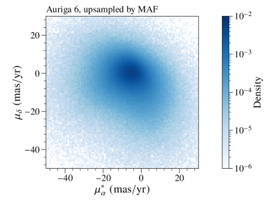
Figure 7: Plots of proper motion for upsampled Auriga 6 stars by MAF within $15^{\circ}$ of the ICRS coordinate $(\alpha,\delta)=(167.47^{\circ},-4.2^{\circ})$ with distance from the assumed Solar location within $3.5$ kpc.

Figure 7 shows the proper motion distribution of stars upsampled by MAF. The proper motion distribution is as smooth as the CNF plot in Figure 3 by eye, suggesting that the MAF also models the distribution well.

A.1 Multi-Model Classifier Test: MAF vs. CNF

To quantitatively compare the upsampling performance of MAF and CNF, we perform the multi-model classifier test. The classifier test is performed in the same way described in Section 5.3 but replacing the EnBiD-upsampled dataset with one from the MAF.

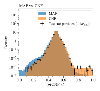
Figure 8: MAF (blue) vs. CNF (orange) classifier output distributions. Black markers are the classifier output histogram of test star particles, which is not used in training upsamplers. Their vertical error bar is $1\sigma$ statistical uncertainty.

We show the classifier output distributions of MAF and CNF-upsampled datasets in Figure 8. Both distributions peak at 0.5, so the two datasets are consistent at some level. However, the distributions are different in both lower and upper tails, and the AUC of this classifier is 0.537, which is slightly higher than 0.5. This indicates that there are non-negligible differences in the details of the distributions. The classifier output distribution of the test star particles is close to that of the CNF-upsampled stars, indicating that CNF can be a better upsampler than MAF.

The log-posterior of the classifier test for MAF vs. CNF is shown in the second column of Table 2. The two scores are much closer than EnBiD vs. CNF since the classifier output distributions are similar. Nevertheless, there is a statistically significant difference between them, and CNF shows a better log-posterior.

We conclude that the density estimate learned by the CNF is more accurate than that learned by the MAF. Note that MAF is essentially a chain of conditional linear transformations that expand and shrink axes, and small wrinkles may appear during the transformation (Huang et al., 2018). Data preprocessing and ensemble averaging may mitigate these effects, but residual artifacts may continue to impact the quality of the density estimation.

Table 2: Log-posteriors from the classifier tests for EnBiD vs. MAF vs. CNF upsampling Auriga 6 star particles. The first two columns are the two-model classifier test results for comparing CNF to the other upsampler. The last column is the results of the multi-model classifier test comparing EnBiD, MAF, and CNF all at once. Large (i.e. less negative) log-posterior scores indicate better upsampling performance. We also show the $1\sigma$ statistical uncertainties of the log-posterior scores, which are taken to be the standard error of the mean log-posterior calculated over the finite-sized test dataset.

Classifier:	EnBiD vs. CNF	MAF vs. CNF	All
Upsampler	$\mathrm{LP}(\mathrm{upsampler})$
EnBiD	$-6.222\pm 0.014$		$-6.894\pm 0.012$
MAF		$-0.7023\pm 0.0002$	$-0.890\pm 0.001$
CNF	$-0.344\pm 0.002$	$-0.6896\pm 0.0002$	$-0.882\pm 0.001$

A.2 Multi-Model Classifier Test: EnBiD vs. MAF vs. CNF

Next, we consider all the upsamplers discussed in this paper: EnBiD, MAF, and CNF, to demonstrate the comparison of multiple upsamplers all at once by our multi-model classifier test.

The classifier output distribution is shown in Figure 9, and we can see all the results we have found from EnBiD vs. CNF and MAF vs. CNF classifier tests. First of all, we can see that the EnBiD distribution is clearly separated from those of MAF, CNF, and reference dataset, which indicates that EnBiD is not performing well compared to the other upsamplers. The other histograms are lying on top of each other because both MAF and CNF are high-performing density estimators. The upsampler generating a distribution closer to that of the reference dataset is CNF, indicating that CNF is better performing than the others.

The log-posteriors are listed in the third column of Table 2. The log-posterior of EnBiD, MAF, and CNF is $-6.89$, $-0.890$, and $-0.882$, respectively. Since CNF shows the largest score value, this multi-model classifier test concludes that CNF is the best upsampler among those three.

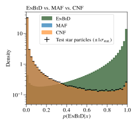
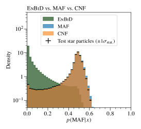
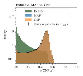
Figure 9: EnBiD (green) vs. MAF (blue) vs. CNF (orange) classifier output distributions. Black markers are the classifier output histogram of test star particles, which is not used in training upsamplers. Their vertical error bar is $1\sigma$ statistical uncertainty.

Appendix B Verification of simplified EnBiD algorithm

In this appendix, we provide further justification for our choice to ignore smoothing steps during EnBiD upsampling. In Figure 10, we show the true Galactocentric velocity, without smearing from measurement errors, for stars in the Aurigaia catalog and our Auriga 6 EnBiD upsampling in the same patch of the sky as Figure 1. For Aurigaia catalog, we remove stars whose progenitor star particles are more than 3.5 kpc away from the Sun in order for a fair comparison to our EnBiD-upsampled dataset. We also overlay a subset of the progenitor star particles from the Auriga 6 simulation. In each plot, we see the same increased concentration of stars around star particles in Galactocentric velocity. The blotches not connected to identified star particles originate from star particles just outside the patch. While the stars in the Aurigaia catalog have a larger spread, we can still visually separate individual clumps. Since this study focuses on this specific feature, we consider our EnBiD upsampling method sufficient. The concentration of stars around star particles also indicates that the proper motion blotchiness in Figure 1 comes from the simulated star particles.

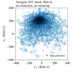
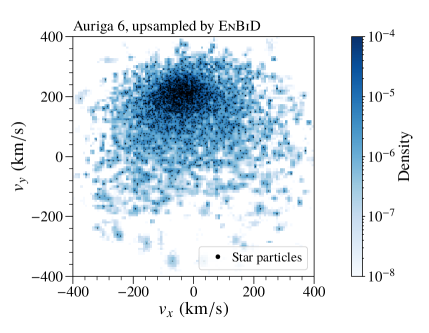
Figure 10: Distributions of Galactocentric velocities $(v_{x},v_{y})$ for Aurigaia (left column) and the Auriga 6 simulation upsampled by EnBiD (right column). We plot all stars within $15^{\circ}$ of the ICRS coordinate $(\alpha,\delta)=(167.47^{\circ},-4.2^{\circ})$ and with distance from the assumed Solar location less than $3.5$ kpc. We further select stars with progenitor star particles within 3.5 kpc from the Sun in order for a fair comparison to our EnBiD-upsampled dataset. Black dots are the progenitor star particles. The distribution for the Aurigaia catalog is shown without measurement errors.

Appendix C Results on Galaxy h277

In this appendix, we apply our upsampling method to the galaxy h277 (Zolotov et al., 2012; Loebman et al., 2012) from the N-Body Shop Collaboration. The galaxy h277 was produced using the Gasoline smoothed particle hydrodynamics code (Wadsley et al., 2004), starting with a dark matter-only simulation within a comoving box with side-length 50 Mpc, and then re-simulating with identical initial conditions at higher resolution including baryons. This simulation has a force resolution of 173 pc, dark matter particle mass of $1.3\times 10^{5}\,M_{\odot}$, initial gas particle mass $2.7\times 10^{4}\,M_{\odot}$, and average star particle mass of $5800\,M_{\odot}$. The entire galaxy has a mass of $7.95\times 10^{11}\,M_{\odot}$ within the virial radius, and was selected as the most Milky Way-like of the galaxies available from this set of simulations. This galaxy currently has no associated mock Gaia catalog, so we here present our upsampler as a first step towards such a catalog.

The star particles within 3.5 kpc from the assumed Solar location, $(-8.122,0.0,0.0208)$ kpc, are selected for training our upsampler. The number of selected star particles is 153,724, and the maximum speed of the selected star particles is 433.79 km/s. We center and re-scale our particles and train a CNF following the procedures outlined in Section 3.

In Figure 11, we show the phase space density distributions in ICRS coordinates for stars upsampled in the angular patch as Figure 1. We additionally overlay the progenitor star particles on each 2D distribution. The patch contains 440 star particles, upsampled to 2,429,709 stars — approximately 5,800 stars per particle or 1 star per $M_{\odot}$. The distributions have no star particle substructure, and the CNF learns the bimodal distance distribution. These plots indicate that upsampling with normalizing flows provides consistent results across multiple simulations.

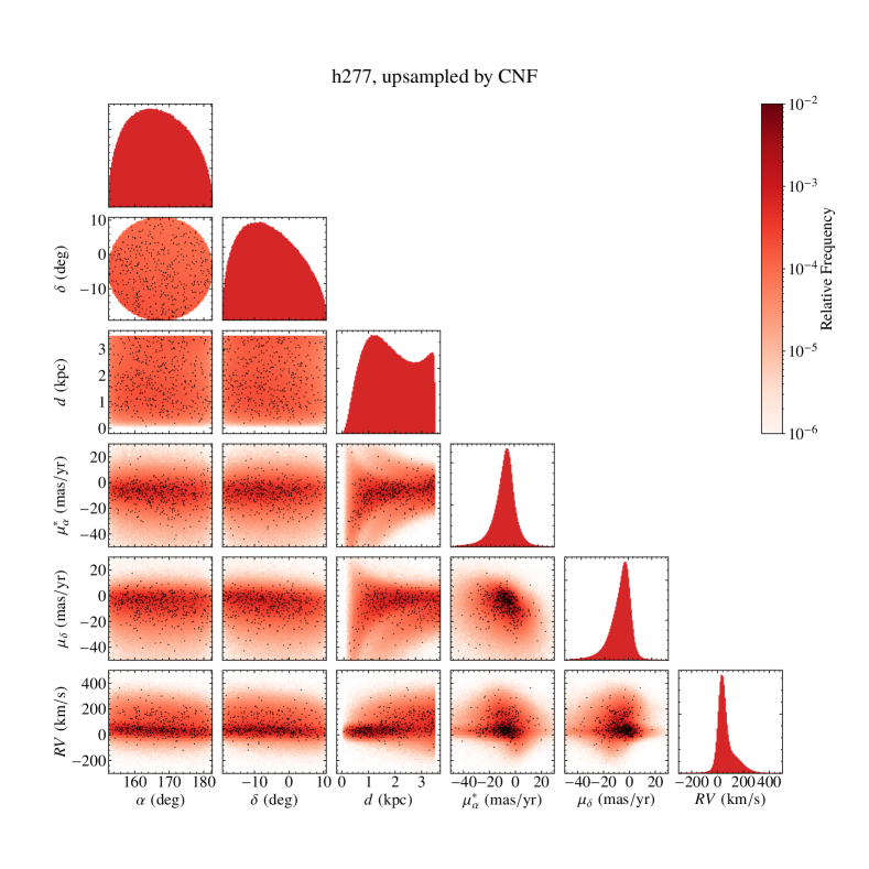
Figure 11: Distributions of CNF-upsampled h277 stars in the ICRS coordinate. We select stars within $15^{\circ}$ from $(\alpha,\delta)=(167.47^{\circ},-4.2^{\circ})$ and with distances from the assumed Solar location less than $3.5$ kpc. The star particles within the selected region are shown as black dots. This patch contains 440 star particles.

Table 3: Log-posteriors from the classifier tests for EnBiD vs. CNF upsampling h277 star particles. Large (i.e. less negative) log-posterior scores indicate better upsampling performance. We also show the $1\sigma$ statistical uncertainties of the log-posterior scores, which are taken to be the standard error of the mean log-posterior calculated over the finite-sized test dataset.

Classifier:	EnBiD vs. CNF
Upsampler	$\mathrm{LP}(\mathrm{upsampler})$
EnBiD	$-9.293\pm 0.032$
CNF	$-0.302\pm 0.004$

We then performed multi-model classifier tests for comparing EnBiD and CNF generated datasets. The log-posteriors of EnBiD and CNf is shown in Table 3. Again, the EnBiD-upsampled dataset contains significant clumps, and the log-posterior of EnBiD is very small: $-9.29$. The log-posterior for CNF is significantly larger than that, and these results again confirm that our GalaxyFlow using CNF is better than EnBiD upsampling.

References

- An et al. (2021) An J., Naik A. P., Evans N. W., Burrage C., 2021, MNRAS, 506, 5721
- Behrmann et al. (2019) Behrmann J., Grathwohl W., Chen R. T. Q., Duvenaud D., Jacobsen J.-H., 2019, in Chaudhuri K., Salakhutdinov R., eds, Proceedings of Machine Learning Research Vol. 97, Proceedings of the 36th International Conference on Machine Learning. PMLR, pp 573–582, https://proceedings.mlr.press/v97/behrmann19a.html
- Boylan-Kolchin et al. (2011) Boylan-Kolchin M., Bullock J. S., Kaplinghat M., 2011, Mon. Not. Roy. Astron. Soc., 415, L40
- Boylan-Kolchin et al. (2012) Boylan-Kolchin M., Bullock J. S., Kaplinghat M., 2012, Mon. Not. Roy. Astron. Soc., 422, 1203
- Brooks & Zolotov (2014) Brooks A. M., Zolotov A., 2014, Astrophys. J., 786, 87
- Brooks et al. (2013) Brooks A. M., Kuhlen M., Zolotov A., Hooper D., 2013, Astrophys. J., 765, 22
- Buckley et al. (2022) Buckley M. R., Lim S. H., Putney E., Shih D., 2022, arXiv e-prints, p. arXiv:2205.01129
- Chen et al. (2018) Chen R. T. Q., Rubanova Y., Bettencourt J., Duvenaud D. K., 2018, in Bengio S., Wallach H., Larochelle H., Grauman K., Cesa-Bianchi N., Garnett R., eds, Vol. 31, Advances in Neural Information Processing Systems. Curran Associates, Inc., https://proceedings.neurips.cc/paper/2018/file/69386f6bb1dfed68692a24c8686939b9-Paper.pdf
- Chen et al. (2019) Chen R. T. Q., Behrmann J., Duvenaud D. K., Jacobsen J.-H., 2019, in Wallach H., Larochelle H., Beygelzimer A., d'Alché-Buc F., Fox E., Garnett R., eds, Vol. 32, Advances in Neural Information Processing Systems. Curran Associates, Inc., https://proceedings.neurips.cc/paper/2019/file/5d0d5594d24f0f955548f0fc0ff83d10-Paper.pdf
- Despali & Vegetti (2017) Despali G., Vegetti S., 2017, Mon. Not. Roy. Astron. Soc., 469, 1997
- Gaia Collaboration et al. (2016) Gaia Collaboration et al., 2016, A&A, 595, A1
- Gaia Collaboration et al. (2018) Gaia Collaboration et al., 2018, A&A, 616, A1
- Gaia Collaboration et al. (2021) Gaia Collaboration et al., 2021, A&A, 649, A1
- Gaia Collaboration et al. (2022) Gaia Collaboration et al., 2022, arXiv e-prints, p. arXiv:2208.00211
- Gardner (2009) Gardner J. P., 2009, in Onaka T., White G. J., Nakagawa T., Yamamura I., eds, Astronomical Society of the Pacific Conference Series Vol. 418, AKARI, a Light to Illuminate the Misty Universe. p. 365
- Garrison-Kimmel et al. (2017) Garrison-Kimmel S., et al., 2017, Mon. Not. Roy. Astron. Soc., 471, 1709
- Grand et al. (2017) Grand R. J. J., et al., 2017, MNRAS, 467, 179
- Grand et al. (2018) Grand R. J. J., et al., 2018, MNRAS, 481, 1726
- Grathwohl et al. (2019) Grathwohl W., Chen R. T. Q., Bettencourt J., Sutskever I., Duvenaud D., 2019, International Conference on Learning Representations
- Green & Ting (2020) Green G. M., Ting Y.-S., 2020, arXiv e-prints, p. arXiv:2011.04673
- Green et al. (2022) Green G. M., Ting Y.-S., Kamdar H., 2022, arXiv e-prints, p. arXiv:2205.02244
- Haber & Ruthotto (2017) Haber E., Ruthotto L., 2017, Inverse Problems, 34, 014004
- Haber et al. (2018) Haber E., Ruthotto L., Holtham E., Jun S.-H., 2018, in Thirty-Second AAAI Conference on Artificial Intelligence.
- Hendrycks & Gimpel (2016) Hendrycks D., Gimpel K., 2016, arXiv e-prints, p. arXiv:1606.08415
- Hopkins (2015) Hopkins P. F., 2015, MNRAS, 450, 53
- Hopkins et al. (2018) Hopkins P. F., et al., 2018, MNRAS, 480, 800
- Huang et al. (2018) Huang C.-W., Krueger D., Lacoste A., Courville A., 2018, in Dy J., Krause A., eds, Proceedings of Machine Learning Research Vol. 80, Proceedings of the 35th International Conference on Machine Learning. PMLR, pp 2078–2087, https://proceedings.mlr.press/v80/huang18d.html
- Kingma & Ba (2014) Kingma D. P., Ba J., 2014, arXiv e-prints, p. arXiv:1412.6980
- Klypin et al. (1999) Klypin A. A., Kravtsov A. V., Valenzuela O., Prada F., 1999, Astrophys. J., 522, 82
- Kobyzev et al. (2021) Kobyzev I., Prince S. J., Brubaker M. A., 2021, IEEE Transactions on Pattern Analysis and Machine Intelligence, 43, 3964
- Krause & Shih (2021) Krause C., Shih D., 2021, arXiv e-prints, p. arXiv:2106.05285
- LSST Dark Energy Science Collaboration (2012) LSST Dark Energy Science Collaboration 2012, arXiv e-prints, p. arXiv:1211.0310
- Loebman et al. (2012) Loebman S. R., Ivezić Ž., Quinn T. R., Governato F., Brooks A. M., Christensen C. R., Jurić M., 2012, ApJ, 758, L23
- Lowing et al. (2014) Lowing B., Wang W., Cooper A., Kennedy R., Helly J., Cole S., Frenk C., 2014, Monthly Notices of the Royal Astronomical Society, 446, 2274
- Lowing et al. (2015) Lowing B., Wang W., Cooper A., Kennedy R., Helly J., Cole S., Frenk C., 2015, MNRAS, 446, 2274
- Lu et al. (2018) Lu Y., Zhong A., Li Q., Dong B., 2018, in Dy J., Krause A., eds, Proceedings of Machine Learning Research Vol. 80, Proceedings of the 35th International Conference on Machine Learning. PMLR, pp 3276–3285, https://proceedings.mlr.press/v80/lu18d.html
- Maas et al. (2013) Maas A. L., Hannun A. Y., Ng A. Y., et al., 2013, in Proc. icml. p. 3
- Moore et al. (1999) Moore B., Ghigna S., Governato F., Lake G., Quinn T. R., Stadel J., Tozzi P., 1999, Astrophys. J. Lett., 524, L19
- Naik et al. (2022) Naik A. P., An J., Burrage C., Evans N. W., 2022, MNRAS, 511, 1609
- Papamakarios et al. (2017) Papamakarios G., Pavlakou T., Murray I., 2017, in Guyon I., Luxburg U. V., Bengio S., Wallach H., Fergus R., Vishwanathan S., Garnett R., eds, Vol. 30, Advances in Neural Information Processing Systems. Curran Associates, Inc., https://proceedings.neurips.cc/paper/2017/file/6c1da886822c67822bcf3679d04369fa-Paper.pdf
- Papamakarios et al. (2021) Papamakarios G., Nalisnick E. T., Rezende D. J., Mohamed S., Lakshminarayanan B., 2021, J. Mach. Learn. Res., 22, 1
- Papastergis et al. (2015) Papastergis E., Giovanelli R., Haynes M. P., Shankar F., 2015, Astron. Astrophys., 574, A113
- Paszke et al. (2019) Paszke A., et al., 2019, in Wallach H., Larochelle H., Beygelzimer A., d'Alché-Buc F., Fox E., Garnett R., eds, Vol. 32, Advances in Neural Information Processing Systems. Curran Associates, Inc., https://proceedings.neurips.cc/paper/2019/file/bdbca288fee7f92f2bfa9f7012727740-Paper.pdf
- (44) Poli M., Massaroli S., Yamashita A., Asama H., Park J., Ermon S., , TorchDyn: Implicit Models and Neural Numerical Methods in PyTorch, https://github.com/DiffEqML/torchdyn
- Pontzen et al. (2013) Pontzen A., Roškar R., Stinson G. S., Woods R., Reed D. M., Coles J., Quinn T. R., 2013, pynbody: Astrophysics Simulation Analysis for Python
- Raissi et al. (2019) Raissi M., Perdikaris P., Karniadakis G., 2019, Journal of Computational Physics, 378, 686
- Robin et al. (2003) Robin A. C., Reylé C., Derrière S., Picaud S., 2003, A&A, 409, 523
- Ruthotto & Haber (2020) Ruthotto L., Haber E., 2020, Journal of Mathematical Imaging and Vision, 62, 352
- Rybizki et al. (2018) Rybizki J., Demleitner M., Fouesneau M., Bailer-Jones C., Rix H.-W., Andrae R., 2018, PASP, 130, 074101
- Sanderson et al. (2020) Sanderson R. E., et al., 2020, ApJS, 246, 6
- Sawala et al. (2013) Sawala T., Frenk C. S., Crain R. A., Jenkins A., Schaye J., Theuns T., Zavala J., 2013, Mon. Not. Roy. Astron. Soc., 431, 1366
- Sawala et al. (2016) Sawala T., et al., 2016, Mon. Not. Roy. Astron. Soc., 457, 1931
- Schaye et al. (2015) Schaye J., et al., 2015, MNRAS, 446, 521
- Sharma & Johnston (2009) Sharma S., Johnston K. V., 2009, ApJ, 703, 1061
- Sharma & Steinmetz (2006) Sharma S., Steinmetz M., 2006, MNRAS, 373, 1293
- Sharma et al. (2011) Sharma S., Bland-Hawthorn J., Johnston K. V., Binney J., 2011, ApJ, 730, 3
- Shih et al. (2022) Shih D., Buckley M. R., Necib L., Tamanas J., 2022, MNRAS, 509, 5992
- Spergel et al. (2015) Spergel D., et al., 2015, arXiv e-prints, p. arXiv:1503.03757
- Springel (2010) Springel V., 2010, ARA&A, 48, 391
- The Dark Energy Survey Collaboration (2005) The Dark Energy Survey Collaboration 2005, arXiv e-prints, pp astro–ph/0510346
- Wadsley et al. (2004) Wadsley J. W., Stadel J., Quinn T., 2004, New Astron., 9, 137
- Wetzel et al. (2016b) Wetzel A. R., Hopkins P. F., Kim J.-h., Faucher-Giguère C.-A., Kereš D., Quataert E., 2016b, ApJ, 827, L23
- Wetzel et al. (2016a) Wetzel A. R., Hopkins P. F., Kim J.-h., Faucher-Giguere C.-A., Keres D., Quataert E., 2016a, Astrophys. J. Lett., 827, L23
- York et al. (2000) York D. G., et al., 2000, AJ, 120, 1579
- Zolotov et al. (2012) Zolotov A., et al., 2012, ApJ, 761, 71