Symplectic Morse Theory: I

Abstract

On manifolds with a specified closed differential form, we introduce a Morse-type cone complex with elements that can be generated by pairs of critical points of a Morse function. The differential of the complex consists of gradient flows and an integration of the closed form over spaces of gradient flow lines. We prove that the cohomology of this complex is independent of both the Riemannian metric and the Morse function used to define the complex. When the specified closed form is a power of the symplectic structure, we prove that the cohomology is isomorphic to the cohomology of differential forms of Tsai, Tseng and Yau (TTY). We also obtain Morse-type inequalities that bound the dimensions of the TTY cohomologies by the number of Morse critical points.

1 Introduction

The Morse complex, also referred to as the Morse-Witten or Smale-Thom complex, captures the information of the standard homology groups of a closed manifold $M$ by means of a Morse function $f$, i.e. a function whose Hessian at each critical point is non-degenerate, and a Riemannian metric $g$. The elements of the complex $C^{k}(M,f)$ are generated by the critical points of $f$, $q\in Crit(f)$, and grouped together by their index, $k=ind(q)$, the number of negative eigenvalues of the Hessian matrix at $q$. The differential of the complex requires the use of the metric and is given by the gradient flow, $-\nabla f$, from one critical point to another. The homology of the Morse complex is well-known to be isomorphic to the standard homology, and therefore, independent of the choice of the Morse function $f$ and the metric $g$. As a corollary of this isomorphism, the Morse inequalities bound the Betti numbers of $M$ in terms of the number of critical points of the Morse function.

We are interested here to consider Morse theory in the presence of a symplectic structure, that is, on a symplectic manifold $(M^{2n},\omega)$. On the cohomology side, besides the de Rham cohomology, Tsai, Tseng and Yau (TTY) [TY1, TY2, TTY] found novel cohomologies of differential forms that can in general vary with the symplectic structure [TY2, GTV, TW]. These cohomologies, labelled by $F^{p}H(M,\omega)$, with $p=0,1,\ldots,n-1$, have interesting properties. In particular, when the symplectic structure is integral class $[\omega]\in H^{2}(M,\mathbb{Z})$, Tanaka and Tseng pointed out that the TTY cohomologies are isomorphic to the de Rham cohomologies of a higher dimensional odd-sphere bundle over the symplectic manifold [TT]. Specifically, denote by $E_{p}$ the bundle $S^{2p+1}\rightarrow E_{p}\rightarrow M$ with Euler class $\omega^{p+1}$, then $F^{p}H(M,\omega)\cong H_{dR}(E_{p})\,$. Certainly, on this odd-sphere bundle, which is a smooth manifold, the dimensions of the de Rham cohomology $H_{dR}(E_{p})$ can be bounded by Morse or Morse-Bott inequalities. This raises the question whether we can modify the standard Morse theory on $(M^{2n},\omega)$ to incorporate the symplectic structure such that we obtain directly Morse-type inequalities for the TTY symplectic cohomologies for any $\omega$, integral class or not.

In this paper, we introduce a set of symplectic Morse complexes for $(M^{2n},\omega)$ defined by a Morse function $f:M\to\mathbb{R}$ and a Riemannian metric $g$ on $M$ whose cohomologies are isomorphic to the TTY symplectic cohomologies.

Our symplectic Morse complex is motivated by a result of Tanaka-Tseng [TT] that relates the cochain complex that underlies the TTY cohomologies with the cone complex of the wedge product map $\omega^{p+1}:\Omega^{\bullet}(M)\to\Omega^{\bullet+2p+2}(M)\,$ on the space of differential forms. Let us recall the general definition of a cone on the de Rham complex.

Definition 1.1.

Let $M$ be a smooth manifold and $\psi\in\Omega^{\ell}(M)$ a degree $\ell$ form that is also $d$-closed. We define the de Rham cone complex of $\psi$, $\text{Cone}(\psi)=(\Omega^{\bullet}(M)\oplus\theta\,\Omega^{\bullet-\ell+1}(M),\,d_{C})$:

where $\theta$ is a formal parameter of degree $(\ell-1)$ and the differential $d_{C}$ can be expressed in matrix form as

$$d_{C}=\begin{bmatrix}d&\psi\\ 0&(-1)^{\ell-1}d\end{bmatrix}\,$$ (1.1)

with $d$ the standard exterior derivative and $\psi$ acting by wedge product.

Note that the $d$-closedness of $\psi$ together with the Leibniz product rule ensures that $d_{C}\,d_{C}=0$. Also, if we formally define $d\theta=\psi\,$, then $d_{C}$ is just the exterior derivative acting on $\Omega^{\bullet}(M)\oplus\theta\,\Omega^{\bullet-\ell+1}(M)$. Of interest, Tanaka-Tseng [TT] proved that on a symplectic manifold $(M^{2n},\omega)$, there is an isomorphism of cohomology for the cone complex when $\psi$ is set to be $\omega^{p+1}$:

$$H({\rm{Cone}}(\omega^{p+1}))\cong F^{p}H(M,\omega)\,,\quad\text{for}~{}p=0,1,\ldots,n-1\,.$$ (1.2)

Motivated by the relationship between de Rham complex and the Morse cochain complex over $\mathbb{R}$, we define in the following a cone Morse complex also over $\mathbb{R}$.

Definition 1.2.

Let $(M,g)$ be an oriented, Riemannian manifold and $f$ a Morse function satisfying the Morse-Smale transversality condition. Let $C^{k}(M,f)$ be the $\mathbb{R}$-module with generators the critical points of $f$ with index $k$. Given a $d$-closed form $\psi\in\Omega^{\ell}(M)$, we define the cone Morse cochain complex of $\psi$, ${\rm{Cone}}(c(\psi))=(C^{\bullet}(M,f)\oplus C^{\bullet-\ell+1}(M,f),\,\partial_{C})$:

with

$$\partial_{C}=\begin{bmatrix}\partial&c(\psi)\\ 0&(-1)^{\ell-1}\partial\end{bmatrix}\,.$$ (1.3)

Here, $\partial$ is the standard Morse cochain differential defined by gradient flow, and $c(\psi):C^{k}(M,f)\to C^{k+l}(M,f)$ acting on a critical point of index $k$ is defined to be

$$c(\psi)\,q_{k}=\sum_{ind(r)={k+l}}\left(\int_{\overline{\mathcal{M}(r_{k+\ell},q_{k})}}\,\psi\right)r_{k+\ell}$$ (1.4)

where $\mathcal{M}(r_{k+\ell},q_{k})$ is the $\ell$-dimensional submanifold of $M$ consisting of all flow lines from the index $k+\ell$ critical point, $r_{k+\ell}\,$, to $q_{k}$.

Notice that the elements of the Morse cone complex, $\text{Cone}^{k}(c(\omega))=C^{k}(M,f)\oplus C^{k-l+1}(M,f)$, can be generated by pairs of critical points of index $k$ and $k-l+1$. The differential $\partial_{C}$ consists of the standard Morse differential $\partial$ from gradient flow couple with the $c(\psi)$ map which involves an integration of $\psi$ over the space of gradient flow lines. This $c(\psi)$ map has appeared in Austin-Braam [AB] and Viterbo [Viterbo] to define a cup product on Morse cohomology. It satisfies the following Leibniz rule

$$\partial c(\psi)+(-1)^{\ell+1}c(\psi)\partial=-c(d\psi)\,.$$ (1.5)

A check of the sign of this equation together with a description of the orientation of $\overline{\mathcal{M}(r_{k+\ell+1},q_{k})}$ is given in Appendix A. With (1.5) and $\partial\partial=0\,,$ they together imply $\partial_{C}\,\partial_{C}=0$.

We will prove in Section 2 that the cohomology of the cone Morse complex ${\rm{Cone}}(c(\psi))$ is isomorphic to the cohomology of the cone complex ${\rm{Cone}}(\psi)$.

Theorem 1.3.

Let $M$ be a closed, oriented manifold and $\psi\in\Omega^{l}(M)$ a $d$-closed form. There exists a chain map ${\cal{P}}_{C}:({\rm{Cone}}^{\bullet}(\psi),d_{C})\to({\rm{Cone}}^{\bullet}(c(\psi)),\partial_{C})$ that is a quasi-isomorphism, and therefore, for any $k\in\mathbb{Z}$,

$$H^{k}({\rm{Cone}}(\psi))\cong H^{k}({\rm{Cone}}(c(\psi)))\,.$$

Theorem 1.3 importantly shows that the cohomology of the cone Morse complex is independent of the choice of both the Morse function and the Riemannian metric used to define ${\rm{Cone}}(c(\psi))$. It is also worthwhile to emphasize that the above theorem is a general one, applicable for any closed smooth manifold, odd or even dimensional.

If we now restrict to a symplectic manifold $(M^{2n},\omega)$, and make use of the isomorphism $H({\rm{Cone}}(\omega^{p+1}))\cong F^{p}H(M,\omega)$ of (1.2), we obtain immediately the following corollary,

Corollary 1.4.

For $(M^{2n},\omega)$ a closed symplectic manifold,

$$H^{k}({\rm{Cone}}(c(\omega^{p+1})))\cong F^{p}H^{k}(M,\omega)\,,$$

for $p=0,1,\dots,n-1\,$.

${\rm{Cone}}(c(\omega^{p+1}))$ thus gives us the desired symplectic Morse complex. The dependence on the symplectic structure is explicit in the differential $\partial_{C}$ which involves the integration of $\omega^{p+1}$ over flow lines between pairs of critical points of the Morse function.

Our cone Morse complex immediately results in Morse-type inequalities. Let us denote by $m_{k}$ the number of Morse critical points with index $k$. We obtain the following:

Theorem 1.5.

Let $M$ be a closed, oriented manifold and $\psi\in\Omega^{\ell}(M)$ a $d$-closed form. Let $b^{\psi}_{k}=\dim{\rm{Cone}}^{k}(\psi)$. Then there exists a polynomial $Q(t)$ with non-negative integer coefficients such that

$$(1+t^{\ell-1})\sum_{k=0}m_{k}\,t^{k}=\sum_{k=0}b^{\psi}_{k}\,t^{k}\,+\,(1+t)\,Q(t)$$ (1.6)

Setting $\psi=\omega^{p+1}$ for the TTY cohomologies, the inequalities of (1.6) are exactly those for the Morse-Bott inequalities on the odd-sphere bundle $E_{p}$ when $\omega$ is integral class. However, we are able to obtain a stronger result when $[\omega]\in H^{2}(M)$ is non-trivial class.

Theorem 1.6.

For a closed symplectic manifold $(M^{2n},\omega)$, let $s_{k}^{p}=\dim F^{p}H^{k}(M,\omega)$. We have the following Morse-type inequalities:
(A) Weak TTY-Morse inequalities

$$s_{k}^{p}\ \leq\,\begin{cases}m_{k}&0\leq k\leq 2p\,,\\ m_{k}+m_{k-2p-1}-1\quad&2p+1\leq k\leq 2n\,,\\ m_{k-2p-1}&2n+1\leq k\leq{2n+2p+1}\,;\\ \end{cases}$$

(B) Strong TTY-Morse inequalities

$$\sum_{i=0}^{k}(-1)^{k-i}s^{p}_{i}\leq\begin{cases}\left(\sum\limits_{i=k-2p}^{k}(-1)^{k-i}m_{i}\right)-1\quad&2p+1\leq k\leq 2n-1,~{}k~{}\text{odd},\\ \sum\limits_{i=k-2p}^{k}(-1)^{k-i}m_{i}&{\text{o}therwise}.\end{cases}$$

Note also that the $s^{p}_{k}\,$’s on the left-hand side of the inequalities may vary with $[\omega]\in H_{dR}^{2}(M)$, while $m_{k}$’s on the right-hand side do not. In fact, the inequalities hold for any Morse function $f$ on $M$.

In a companion paper [CTT], we will provide an analytic proof using Witten deformation method to the isomorphism in Corollary 1.4 and the Morse-type inequalities for the TTY cohomologies.

Note added: After we had obtained the Morse-type inequalities (1.6) for the TTY cohomologies, a preprint [Machon] appeared which has some relation to the symplectic Morse-type inequalities given in this work. However, the inequalities in [Machon] differ from those here and in fact do not hold in general as explained in Remark 3.5.

Acknowledgements.  We thank Hiro Lee Tanaka, Weiping Zhang, and Jiawei Zhou for helpful discussions. The second author was supported in part by NSF Grants DMS-1800666 and DMS-1952551. The third author would like to acknowledge the support of the Simons Collaboration Grant No. 636284.

2 Morse cone complex: Cone(c($\psi$))

2.1 Preliminaries: Morse complex and $c(\psi)$

To begin, let $f$ be a Morse function and $g$ a Riemannian metric on $M$. We will assume throughout this paper that $(f,g)$ satisfy the standard Morse-Smale transversality condition. The elements of the Morse cochain complex $C^{\bullet}(M,f)$ are $\mathbb{R}$-modules with generators critical points of $f$, graded by the index of the critical points, with boundary operator $\partial$ determined by the counting of gradient lines, i.e

$$\partial q_{k}=\displaystyle\sum_{ind(r)=k+1}n(r_{k+1},q_{k})\,r_{k+1},$$

where $n(r_{k+1},q_{k})=\#\widetilde{\mathcal{M}}(r_{k+1},q_{k})$ is a count of the moduli space of gradient flow lines with orientation modulo reparametrization.

Note that Morse theory is typically presented as a homology theory, and hence, flowing from index $k$ to index $k-1$ critical points. To match up with the cochain complex of differential forms, we here work with the dual Morse cochain complex. Hence, our $\partial$ is the adjoint of the usual Morse boundary map under the inner product $\langle q_{k_{i}},q_{k_{j}}\rangle=\delta_{ij}$.

Following Austin-Braam [AB] and Viterbo [Viterbo], we define

$$c(\psi)q_{k}=\displaystyle\sum_{ind(r)=k+\ell}\left(\int_{\overline{\mathcal{M}(r_{k+\ell},q_{k})}}\psi\right)r_{k+\ell}$$

where $\psi\in\Omega^{\ell}(M)$ is an $\ell$-form and $\mathcal{M}(r_{k+\ell},q_{k})$ is the submanifold of all points that flow from $r_{k+\ell}$ to $q_{k}$, oriented as in [AB]. From Appendix A, we have the Leibniz-type product relation

$$\partial c(\psi)+(-1)^{\deg(\psi)+1}c(\psi)\partial=-c(d\psi)$$

specifying a sign convention that is ambiguous in Austin-Braam [AB] and Viterbo [Viterbo]. Thus, for instance, for $\psi=\omega$, the symplectic structure, we have the relation

$$\partial c(\omega)-c(\omega)\partial=-c(d\omega)=0$$

2.2 Chain map between $\textnormal{Cone}(\psi)$ and Cone$(c(\psi))$

As explained by Bismut, Zhang and Laudenbach [BZ, Zhang], there is a chain map ${\cal{P}}:\Omega^{k}(M)\to C^{k}(M,f)$ between differential forms and the Morse cochain complex given by

$${\cal{P}}\phi=\sum_{q_{k}\in Crit(f)}\left(\int_{\overline{U_{q_{k}}}}\phi\right)q_{k}$$

where $\phi\in\Omega^{k}(M)$ and $U_{q}$ is the set of all points on a gradient flow away from $q$. Being a chain map,

$$\partial\,{\cal{P}}={\cal{P}}\,d\,.$$ (2.1)

We are interested to find an analogous chain map relating $\text{Cone}(\psi)=(\Omega^{\bullet}(M)\oplus\theta\,\Omega^{\bullet-\ell+1}(M),\,d_{C})$ with ${\rm{Cone}}(\psi)=(C^{\bullet}(M,f)\oplus C^{\bullet-\ell+1}(M,f),\,\partial_{C})$, where as given in Definition 1.1 and Definition 1.2,

$$d_{C} :\Omega^{k}(M)\oplus\theta\,\Omega^{k-l+1}(M)\to\Omega^{k+1}(M)\oplus\theta\,\Omega^{k-l+2}(M)$$

$$\partial_{C} :C^{k}(M,f)\oplus C^{k-l+1}(M,f)\to C^{k+1}(M,f)\oplus\,C^{k-l+2}(M,f)$$

with

$$d_{C}=\begin{bmatrix}d&\psi\\ 0&(-1)^{\ell-1}d\end{bmatrix}\,,\qquad\partial_{C}=\begin{bmatrix}\partial&c(\psi)\\ 0&(-1)^{\ell-1}\partial\end{bmatrix}\,.$$

The chain map, which we will label by ${\cal{P}}_{C}$, that links the two cone complexes will need to satisfy $\partial_{C}\,{\cal{P}}_{C}={\cal{P}}_{C}\,d_{C}$. In fact, such a map exists and can be expressed in an upper-triangular matrix form.

Definition 2.1.

Let ${\cal{P}}_{C}:{\rm{Cone}}^{\bullet}(\psi)\to{\rm{Cone}}^{\bullet}(c(\psi))$ be the upper-triangular matrix map

$${\cal{P}}_{C}=\begin{bmatrix}{\cal{P}}&K\\ 0&{\cal{P}}\end{bmatrix}$$

where $K:\Omega^{k-\ell+1}(M)\to C^{k}(M,f)$ acting on $\xi\in\Omega^{k-\ell+1}(M)$ is defined by

$$K\xi=(-1)^{\ell}\left[{\cal{P}}(\psi\wedge d^{*}G\xi)-c(\psi){\cal{P}}(d^{*}G\xi)\right]+\partial_{k,\perp}^{-1}({\cal{P}}(\psi\wedge\mathcal{H}\xi)-c(\psi){\cal{P}}(\mathcal{H}\xi))\,,$$ (2.2)

in terms of the Hodge decomposition with respect to the de Rham Laplacian $\Delta=dd^{*}+d^{*}d$:

$$\xi=(\mathcal{H}+\Delta G)\xi=\mathcal{H}\xi+dd^{*}G\xi+d^{*}dG\xi\,,$$

where $\mathcal{H}\xi$ is the harmonic component and $G$ is the Green’s operator.

We explain the notation $\partial_{k,\perp}^{-1}$ in the second term for the definition of $K$ in (2.2).

Let $\gamma$ be a closed $(k-\ell+1)$-form. Then, it is known that ${\cal{P}}\psi\wedge\gamma$ and $c(\psi){\cal{P}}\gamma$ are cohomologous. (See, for instance, Austin-Braam [AB, Section 3.5] or Viterbo [Viterbo, Lemma 4].). Then ${\cal{P}}(\psi\wedge\gamma)-c(\psi){\cal{P}}\gamma=\partial b$ for some $b\in C^{k}(M,f)$. Note that $C^{k}(M,f)$ is an inner product space under $\langle q_{k_{i}},q_{k_{j}}\rangle=\delta_{ij}$, so we have an orthogonal splitting, $C^{k}(M,f)=\ker\partial_{k}\oplus(\ker\partial_{k})^{\perp}$, and that $\partial_{k}$ is an isomorphism between $\text{Im}(\partial_{k})\subset C^{k+1}(M,f)$ and $C^{k}(M,f)/\ker\partial_{k}$, which is isomorphic to $(\ker\partial_{k})^{\perp}$. Thus, it follows from the finite-dimensional assumption on $C^{k}(M,f)$ and $C^{k+1}(M,f)$ that we can define a right inverse $\partial_{k,\perp}^{-1}:\text{Im}(\partial_{k})\to(\ker\partial_{k})^{\perp}\subset C^{k}(M,f)$, and $\partial_{k,\perp}^{-1}({\cal{P}}(\psi\wedge\gamma)-c(\psi){\cal{P}}\gamma)\in C^{k}(M,f)$. For the second term of $K$ in (2.2), $\gamma=\mathcal{H}\xi$ is the closed form that is the harmonic component of $\xi$.

With ${\cal{P}}_{C}$ defined, we now show that it is a chain map.

Theorem 2.2.

${\cal{P}}_{C}:{\rm{Cone}}^{\bullet}(\psi)\to{\rm{Cone}}^{\bullet}(c(\psi))$ is a chain map. In particular,

$$\partial_{C}\,{\cal{P}}_{C}={\cal{P}}_{C}\,d_{C}\,.$$ (2.3)

Proof.

The right and the left hand side of (2.3) acting on $\eta+\theta\xi\in Cone^{k}(\psi)$ give

$${\cal{P}}_{C}\,d_{C} =\begin{bmatrix}{\cal{P}}&K\\ 0&{\cal{P}}\end{bmatrix}\begin{bmatrix}d&\psi\\ 0&(-1)^{\ell-1}d\end{bmatrix}=\begin{bmatrix}{\cal{P}}d&{\cal{P}}\psi+(-1)^{\ell-1}Kd\\ 0&(-1)^{\ell-1}{\cal{P}}d\end{bmatrix},$$

$$\partial_{C}\,{\cal{P}}_{C} =\begin{bmatrix}\partial&c(\psi)\\ 0&(-1)^{\ell-1}\partial\end{bmatrix}\begin{bmatrix}{\cal{P}}&K\\ 0&{\cal{P}}\end{bmatrix}=\begin{bmatrix}\partial{\cal{P}}&c(\psi){\cal{P}}+\partial K\\ 0&(-1)^{\ell-1}\partial{\cal{P}}\end{bmatrix}.$$

Since ${\cal{P}}$ is a chain map (2.1), i.e. $d\,{\cal{P}}={\cal{P}}\,\partial$, the only entry we need to check comes from the off-diagonal one,

$${\cal{P}}\psi+(-1)^{\ell-1}Kd=c(\psi){\cal{P}}+\partial K\,,$$

or equivalently, we need to show that

$${\cal{P}}\psi-c(\psi){\cal{P}}=\partial K+(-1)^{\ell}Kd\,,$$ (2.4)

is a graded chain homotopy. To compute $Kd\xi$, note first that $\mathcal{H}d\xi=0\,$, $\forall\xi\in\Omega^{k-l+1}(M).$ Therefore, we find that

$$Kd\xi=(-1)^{\ell}\left[{\cal{P}}(\psi\wedge d^{*}Gd\xi)-c(\psi){\cal{P}}d^{*}Gd\xi\right]=(-1)^{\ell}\left[{\cal{P}}(\psi\wedge d^{*}dG\xi)-c(\psi){\cal{P}}d^{*}dG\xi\right]\,,$$

having used (2.2) and the fact that $Gd=dG$. Now, for the $\partial K\xi$ term, we have

$$\partial K\xi =\partial\left((-1)^{\ell}\left[{\cal{P}}(\psi\wedge d^{*}G\xi)-c(\psi){\cal{P}}d^{*}G\xi\right]+\partial_{k,\perp}^{-1}({\cal{P}}(\psi\wedge\mathcal{H}\xi)-c(\psi){\cal{P}}\mathcal{H}\xi)\right)$$

$$=(-1)^{\ell}\left[{\cal{P}}d(\psi\wedge d^{*}G\xi)-\partial c(\psi){\cal{P}}d^{*}G\xi\right]+\partial\left(\partial_{k,\perp}^{-1}({\cal{P}}(\psi\wedge\mathcal{H}\xi)-c(\psi){\cal{P}}\mathcal{H}\xi)\right)$$

$$=(-1)^{\ell}\left[(-1)^{\ell}{\cal{P}}(\psi\wedge dd^{*}G\xi)-(-1)^{\ell}c(\psi)\partial{\cal{P}}d^{*}G\xi\right]+{\cal{P}}\psi\wedge\mathcal{H}\xi-c(\psi){\cal{P}}\mathcal{H}\xi$$

$$={\cal{P}}(\psi\wedge dd^{*}G\xi)-c(\psi){\cal{P}}dd^{*}G\xi+{\cal{P}}(\psi\wedge\mathcal{H}\xi)-c(\psi){\cal{P}}\mathcal{H}\xi$$

Altogether, we find for the right-hand side of (2.4)

$$\partial K\xi+(-1)^{\ell}Kd\xi ={\cal{P}}(\psi\wedge dd^{*}G\xi)-c(\psi){\cal{P}}dd^{*}G\xi+{\cal{P}}(\psi\wedge\mathcal{H}\xi)-c(\psi){\cal{P}}\mathcal{H}\xi$$

$$\qquad+\left[{\cal{P}}(\psi\wedge d^{*}dG\xi)-c(\psi){\cal{P}}d^{*}dG\xi\right]$$

$$={\cal{P}}\left(\psi\wedge(dd^{*}G\xi+d^{*}dG\xi+\mathcal{H}\xi)\right)-c(\psi){\cal{P}}(dd^{*}G\xi+d^{*}dG\xi+\mathcal{H}\xi)$$

$$={\cal{P}}(\psi\wedge\xi)-c(\psi){\cal{P}}\xi.$$

Thus, $K$ is a graded chain homotopy of ${\cal{P}}\psi$ and $c(\psi){\cal{P}}$, and therefore, ${\cal{P}}_{C}\,d_{C}=\partial_{C}\,{\cal{P}}_{C}$. ∎

2.3 Isomorphism of cohomologies via Five Lemma

A mapping cone cochain complex can be described by a short exact sequence of chain maps. For the differential forms case, we have

(2.5)

where $\iota$ is the inclusion in the first component $\iota(a)=\begin{bmatrix}a\\ 0\end{bmatrix}$ and $\pi$ is the projection to the second component $\pi\left(\begin{bmatrix}a\\ b\end{bmatrix}\right)=b$. It is easy to check that these maps are chain maps:

$$\iota_{dR}d\eta=\begin{bmatrix}d\eta\\ 0\end{bmatrix}=d_{C}\iota_{dR}\eta$$

and

$$\pi_{dR}d_{C}\left(\begin{bmatrix}\eta\\ \xi\end{bmatrix}\right)=\pi_{dR}\begin{bmatrix}d\eta+\psi\wedge\xi\\ (-1)^{\ell-1}d\xi\end{bmatrix}=(-1)^{\ell-1}d\xi=(-1)^{\ell-1}d\left(\pi_{dR}\begin{bmatrix}\eta\\ \xi\end{bmatrix}\right)\,.$$

The short exact sequence (2.5) implies the following long exact sequence for the cohomology of Cone$(\psi)$

(2.6)

Analogously, for Cone($c(\psi))$, we also have the short exact sequence of chain maps

(2.7)

and the long exact sequence of cohomology

(2.8)

The two short exact sequences, (2.5) and (2.7), fit into a commutative diagram

(2.9)

The commutativity can be checked as follows:

$$\iota_{C(f)}({\cal{P}}(\eta))=\begin{bmatrix}{\cal{P}}\eta\\ 0\end{bmatrix}=\begin{bmatrix}{\cal{P}}&K\\ 0&{\cal{P}}\end{bmatrix}\begin{bmatrix}\eta\\ 0\end{bmatrix}={\cal{P}}_{C}(\iota_{dR}(\eta))\,,$$

$$\pi_{C(f)}\left({\cal{P}}_{C}\begin{bmatrix}\eta\\ \xi\end{bmatrix}\right)=\pi_{C(f)}\begin{bmatrix}{\cal{P}}\eta+K\xi\\ {\cal{P}}\xi\end{bmatrix}={\cal{P}}\xi={\cal{P}}\left(\pi_{dR}\begin{bmatrix}\eta\\ \xi\end{bmatrix}\right).$$

The short exact commutative diagram (2.9) gives a long commutative diagram of cohomologies:

(2.10)

We can check that each square commutes. The outer squares commute since ${\cal{P}}(\psi\wedge\xi)$ and $c(\psi){\cal{P}}\xi$ are cohomologous when both $\xi$ and $\psi$ are $d$-closed, i.e.

$$[{\cal{P}}][\psi\wedge]=[c(\psi)][{\cal{P}}]$$

as was shown by Austin-Braam in [AB, Section 3.5]. The middle two squares commute follows from the commutativity of the chain maps in (2.9). Furthermore, the vertical map $[{\cal{P}}]$ is an isomorphism as shown by Bismut-Zhang and Laudenbach [BZ, Theorem 2.9] (see also [Zhang, Theorem 6.4]).

We can now apply the Five Lemma to (2.10) which implies that the middle vertical map $[{\cal{P}}_{C}]$ is also an isomorphism on cohomology, and thus we prove Theorem 1.3.

Theorem 2.3.

${\cal{P}}_{C}:({\rm{Cone}}^{\bullet}(\psi),d_{C})\to({\rm{Cone}}^{\bullet}(c(\psi)),\partial_{C})$ is a $\mathbb{Z}$ graded quasi-isomorphism.

2.4 Example: Cone$(c(\omega))$ on $T^{4}$

We now work out a simple example of the Cone$(c(\psi))$ complex on the four-dimensional torus, $M=T^{4}=\mathbb{R}^{4}/\mathbb{Z}^{4}$. We will describe the torus using Euclidean coordinates, $x_{i}$ with $i=1,2,3,4,$ with identification $x_{i}\sim x_{i}+1$. We are interested in the symplectic case where $\psi=\omega=dx_{1}\wedge dx_{2}+dx_{3}\wedge dx_{4}$.

The complex ${\rm{Cone}}(c(\omega))$ is dependent on the choice of the metric and the Morse function. For simplicity, we will work with the flat metric, $g=\sum dx_{i}^{2}$ and choose the Morse function to be

$$f=2-\frac{1}{2}\sum_{i=1}^{4}\cos(2\pi x_{i})\,.$$

This Morse function has several desirable properties that are straightforward to prove:

• the non-degenerate critical points are located at $x_{i}=[0]$ or $x_{i}=[\tfrac{1}{2}]$ and have Morse index equal to the number of coordinates which are equal to $[\tfrac{1}{2}]$;

• the Morse differential $\partial$ is 0;

• the pair $(f,g)$ is Morse-Smale.

Because of (ii), the $\partial_{C}$ map in (1.3) reduces to the $c(\omega)$ map. Hence, we are interested in pairs of critical points whose indices differ by two, e.g $q_{k+1}$ has two more $[\tfrac{1}{2}]$ coordinates than $q_{k-1}$. Also, note that $\mathcal{M}(q_{k+1},q_{k-1})$ will be a two-dimensional face with two of the coordinates fixed and two coordinates spanning the entire coordinate interval $[0,1]$ when we take the closure.

In the Table 1 below, we give the cohomologies of $H({\rm{Cone}}(c(\omega)))$ and $H({\rm{Cone}}(\omega))$ on $(T^{4},\omega=dx_{1}\wedge dx_{2}+dx_{3}\wedge dx_{4})$. We use a multi-index notation of $I=\{i_{1}...i_{j}\}$ in increasing order such that $dx_{I}=dx_{i_{1}}\wedge...\wedge dx_{i_{j}}$, $q_{0}$ denotes the index 0 point, and $q_{I}$ denotes the point with $\tfrac{1}{2}$ in entry $i_{1},...i_{j}$, i.e. $q_{13}=q_{\left[\tfrac{1}{2},0,\tfrac{1}{2},0\right]}$. The orientation of the submanifolds are chosen such that ${\cal{P}}dx_{I}=q_{I}$. Further, since $\partial=0$ and $G\,dx_{I}=0$, we also have $K\,dx_{I}=0\,$.

Notice that $c(\omega)q_{I}$ only picks out critical points that have two coordinates of $q_{I}$ changed from $[0]$ to $[\tfrac{1}{2}]$ in either the 1-2 or 3-4 directions. Thus, we find that

$$c(\omega)q_{0} =q_{12}+q_{34}\,, c(\omega)q_{12} =q_{1234}\,, c(\omega)q_{34} =q_{1234}\,,$$

$$c(\omega)q_{1} =q_{134}\,, c(\omega)q_{2} =q_{234}\,, c(\omega)q_{3} =q_{123}\,, c(\omega)q_{4} =q_{124}\,,$$

with all other critical points mapped to zero when acted upon by $c(\omega)$.

$j$ $0$ $1$ $2$ $H^{j}(\text{Cone}(\omega))$ $\begin{bmatrix}1\\ 0\end{bmatrix}$ $\begin{bmatrix}dx_{1}\\ 0\end{bmatrix},\begin{bmatrix}dx_{2}\\ 0\end{bmatrix}$ $\begin{bmatrix}dx_{13}\\ 0\end{bmatrix},\begin{bmatrix}dx_{14}\\ 0\end{bmatrix},\begin{bmatrix}dx_{23}\\ 0\end{bmatrix},$ $\begin{bmatrix}dx_{3}\\ 0\end{bmatrix},\begin{bmatrix}dx_{4}\\ 0\end{bmatrix}$ $\begin{bmatrix}dx_{24}\\ 0\end{bmatrix},\begin{bmatrix}dx_{12}-dx_{34}\\ 0\end{bmatrix}$ $H^{j}(\text{Cone}(c(\omega)))$ $\begin{bmatrix}q_{0}\\ 0\end{bmatrix}$ $\begin{bmatrix}q_{1}\\ 0\end{bmatrix},\begin{bmatrix}q_{2}\\ 0\end{bmatrix}$ $\begin{bmatrix}q_{13}\\ 0\end{bmatrix},\begin{bmatrix}q_{14}\\ 0\end{bmatrix},\begin{bmatrix}q_{23}\\ 0\end{bmatrix},$ $\begin{bmatrix}q_{3}\\ 0\end{bmatrix},\begin{bmatrix}q_{4}\\ 0\end{bmatrix}$ $\begin{bmatrix}q_{24}\\ 0\end{bmatrix},\begin{bmatrix}q_{12}-q_{34}\\ 0\end{bmatrix}$         $j$ $3$ $4$ $5$ $H^{j}(\text{Cone}(\omega))$ $\begin{bmatrix}dx_{123}\\ 0\end{bmatrix},\begin{bmatrix}dx_{124}\\ 0\end{bmatrix},\begin{bmatrix}dx_{234}\\ 0\end{bmatrix},$ $\begin{bmatrix}0\\ dx_{123}\end{bmatrix},\begin{bmatrix}0\\ dx_{124}\end{bmatrix}$ $\begin{bmatrix}0\\ dx_{1234}\end{bmatrix}$ $\begin{bmatrix}dx_{234}\\ 0\end{bmatrix},\begin{bmatrix}0\\ dx_{12}-dx_{34}\end{bmatrix}$ $\begin{bmatrix}0\\ dx_{134}\end{bmatrix},\begin{bmatrix}0\\ dx_{234}\end{bmatrix}$ $H^{j}(\text{Cone}(c(\omega)))$ $\begin{bmatrix}q_{123}\\ 0\end{bmatrix},\begin{bmatrix}q_{124}\\ 0\end{bmatrix},\begin{bmatrix}q_{234}\\ 0\end{bmatrix},$ $\begin{bmatrix}0\\ q_{123}\end{bmatrix},\begin{bmatrix}0\\ q_{124}\end{bmatrix}$ $\begin{bmatrix}0\\ q_{1234}\end{bmatrix}$ $\begin{bmatrix}q_{234}\\ 0\end{bmatrix},\begin{bmatrix}0\\ q_{12}-q_{34}\end{bmatrix}$ $\begin{bmatrix}0\\ q_{134}\end{bmatrix},\begin{bmatrix}0\\ q_{234}\end{bmatrix}$

Table 1: Cohomology of Cone$(\omega)$ versus Cone$(c(\omega))$ on $(T^{4},\omega=dx_{1}\wedge dx_{2}+dx_{3}\wedge dx_{4})$.

3 Cone and symplectic Morse inequalities

Having established the quasi-isomorphism between the complexes, Cone$(\psi)$ and Cone$(c(\psi))$, we proceed now to write down the associated Morse-type inequalities.

We recall first the standard Morse inequalities (for a reference, see [Milnor]). Let $m_{k}$ be the number of index $k$ critical points of a Morse function, and $b_{k}=\dim H^{k}(M)$, the $k$-th Betti number. The Morse inequalities can be stated as the existence of a polynomial $Q(t)$ with non-negative integer coefficients such that

$$\sum_{k=0}m_{k}\,t^{k}=\sum_{k=0}b_{k}\,t^{k}\,+\,(1+t)\,Q(t)\,.$$ (3.1)

This is equivalent to what is sometimes called the strong Morse inequalities

$$\sum_{i=0}^{k}(-1)^{k-i}\,b_{i}\,\leq\,\sum_{i=0}^{k}(-1)^{k-i}\,m_{i}\,,\qquad k=0,\ldots,\dim M$$ (3.2)

which implies the weak Morse inequalities

$$b_{k}\leq m_{k}\,,$$ (3.3)

also for $k=0,\ldots,\dim M\,$.

In Theorem 1.5, we wrote down the polynomial form (analogous to (3.1)) for the Morse-type inequalities of the Cone$(\psi)$ complex. However, the weak and strong forms are perhaps more explicit and easier to use, and so we will below give the proof of the cone Morse inequalities in the weak and strong forms.

Proposition 3.1.

For a closed, oriented manifold $M$ and a $d$-closed form $\psi\in\Omega^{l}(M)$, let $b_{k}^{\psi}=\dim H^{k}(\text{Cone}(\psi))$. Let $m_{k}$ be the number of index $k$ critical points of a Morse function. Then, we have the following inequalities for $k=0,1,\ldots,(\dim M+\ell-1)$:

(A) Weak Morse-type inequalities

$$b_{k}^{\psi}\leq m_{k}+m_{k-\ell+1}\,;$$ (3.4)

(B) Strong Morse-type inequalities

$$\sum_{i=0}^{k}(-1)^{k-i}b_{i}^{\psi}\leq\sum_{i=0}^{k}(-1)^{k-i}(m_{i}+m_{i-\ell+1})\,.$$ (3.5)

Proof.

For (A), since $\text{Cone}^{k}(\psi)=C^{k}(M,f)\oplus C^{k-\ell+1}(M,f)$ is finitely generated, the dimension of $H^{k}(\text{Cone}(c(\psi)))$ is bounded by the number of generators of $\text{Cone}^{k}(c(\psi))$ which immediately gives us the weak inequalities

$$b_{k}^{\psi}=\dim(H^{k}(\text{Cone}(\psi)))\leq\dim((\text{Cone}^{k}(\psi))=m_{k}+m_{k-\ell+1}\,.$$

For (B), we can apply the strong Morse inequalities relations (see, for example, [Zhang, Section 5.5]) to the finite-dimensional Cone$(c(\psi))$ complex. This gives

$$\sum_{i=0}^{k}(-1)^{k-i}b^{\psi}_{i}\leq\sum_{i=0}^{k}(-1)^{k-i}\dim({\rm{Cone}}^{i}(c(\psi)))=\sum_{i=0}^{k}(-1)^{k-i}(m_{i}+m_{i-\ell+1})\,.$$

∎

Note that the strong Morse-type inequalities (3.5) can be expressed in simpler forms depending on the value of $\ell=deg(\psi)$.

$$\sum_{i=0}^{k}(-1)^{k-i}b^{\psi}_{i}\leq\begin{cases}(-1)^{k}m_{0}+m_{k+1}&\ell=0\,,\\ 2\sum\limits_{i=0}^{k}(-1)^{k-i}\,m_{i}&\ell=1\,,\\ \sum\limits_{i=k-\ell+2}^{k}(-1)^{k-i}\,m_{i}&\ell~{}\text{even},\,\ell\geq 2\,,\\ \sum\limits_{i=k-\ell+2}^{k}(-1)^{k-i}\,m_{i}+2\sum\limits_{i=0}^{k}m_{i-\ell+1}\quad&\ell~{}\text{odd},\,\ell\geq 3\,.\end{cases}$$ (3.6)

In the symplectic case, where $\psi=\omega^{p+1}$ and $H({\rm{Cone}}(\omega^{p+1}))\cong F^{p}H(M,\omega)$, let us denote by $s^{p}_{k}=\dim F^{p}H^{k}(M,\omega)=\dim H^{k}({\rm{Cone}}(\omega^{p+1}))$, the dimension of the TTY cohomology. When $[\omega]\in H^{2}_{dR}(M)$ is non-trivial, we can obtain inequalities stronger than (3.4)-(3.5) by applying standard Morse inequalities (3.2)-(3.3) to the algebraic relation

$$H^{k}(\text{Cone}(\omega^{p+1})) \cong\text{coker}\left([\omega^{p+1}]:H^{k-2p-2}(M)\to H^{k}(M)\right)$$

$$\quad\quad\oplus\,\ker\left([\omega^{p+1}]:H^{k-2p-1}(M)\to H^{k+1}(M)\right)$$ (3.7)

which follows from (2.6) (see also [TTY, Corollary 4.3]). We find the following.

Theorem 3.2.

For a closed symplectic manifold $(M^{2n},\omega)$, let $s_{k}^{p}=\dim F^{p}H^{k}(M,\omega)$ with $p=0,1,\ldots,n-1$ and $k=0,1,\ldots,2n+2p+1$. Let $m_{j}$ be the number of index $j$ critical points of a Morse function. Then, we have the following Morse-type inequalities:
(A) Weak TTY-Morse inequalities

$$s_{k}^{p}\ \leq\,\begin{cases}m_{k}&0\leq k\leq 2p\,,\\ m_{k}+m_{k-2p-1}-1\quad&2p+1\leq k\leq 2n\,,\\ m_{k-2p-1}&2n+1\leq k\leq{2n+2p+1}\,;\\ \end{cases}$$ (3.8)

(B) Strong TTY-Morse inequalities

$$\sum_{i=0}^{k}(-1)^{k-i}s^{p}_{i}\leq\begin{cases}\left(\sum\limits_{i=k-2p}^{k}(-1)^{k-i}m_{i}\right)-1\quad&2p+1\leq k\leq 2n-1,~{}~{}k~{}\text{odd},\\ \sum\limits_{i=k-2p}^{k}(-1)^{k-i}m_{i}&\text{otherwise}.\\ \end{cases}$$ (3.9)

Proof.

For (A), we begin by bounding the dimensions of the kernel and cokernel in (3). Specifically, with $b_{k}=\dim H^{k}(M)$ denoting the $k$-th Betti number, we have

$$\dim\text{coker}\left([\omega^{p+1}]:H^{k-2p-2}(M)\to H^{k}(M)\right)\leq\dim(H^{k}(M))=b_{k}\leq m_{k}$$ (3.10)

$$\dim\ker\left([\omega^{p+1}]:H^{k-2p-1}(M)\to H^{k+1}(M)\right)\leq\dim(H^{k-2p-1}(M))=b_{k-2p-1}\leq m_{k-2p-1}$$ (3.11)

having used the standard weak inequalities (3.3). Therefore, we obtain

$$s^{p}_{k}\leq m_{k}+m_{k-2p-1}\,,$$ (3.12)

which is exactly the weak inequality in (3.4) for $\psi=\omega^{p+1}$. Note that when $k\leq 2p$ or $k\geq 2n+1$, one of the two terms in (3.12) vanishes. Hence, to complete the proof of (3.8), it remains to show that when $2p+1\leq k\leq 2n$, the bound in (3.12) can be decreased by minus one. This follows from noting that $[\omega^{r}]\in H^{2r}(M)$, for $r=0,1,\dots,n,$ are all non-trivial classes on a closed symplectic manifold. Therefore, the map $[\omega^{p+1}]:[\omega^{r-p-1}]\to[\omega^{r}]$ is bijective as long as $0\leq r-p-1$ and $r\leq n$. We can thus improve the bound in (3.10)-(3.11) by removing these powers of $\omega$ generators. In particular, for (3.10), when $k$ is even and $2p+2\leq k\leq 2n$, the bound for the cokernel map can be decreased by one. Similarly, for (3.11), the bound for the kernel map can be decreased by one when $k$ is odd and $2p+1\leq k\leq 2n-1$. Altogether, we obtain the bound

$$s^{p}_{k}\leq m_{k}+m_{k-2p-1}-1\,,\qquad 2p+1\leq k\leq 2n\,.$$

To prove (B), we will use the notation $[\omega^{p+1}]_{i}$ to denote the map $[\omega^{p+1}]_{i}:H^{i}(M)\to H^{i+2p+2}(M)$. It then follows from (3) that

$$\sum_{i=0}^{k}(-1)^{k-i}s^{p}_{i} =\sum_{i=0}^{k}(-1)^{k-i}\left(\dim\text{coker}[\omega^{p+1}]_{i-2p-2}+\dim\ker[\omega^{p+1}]_{i-2p-1}\right)$$

$$=\sum_{i=0}^{k}(-1)^{k-i}\left(\dim\text{coker}[\omega^{p+1}]_{i-2p-2}-\dim\ker[\omega^{p+1}]_{i-2p-2}\right)$$

$$\qquad+\dim\ker[\omega^{p+1}]_{k-2p-1}$$

$$=\sum_{i=0}^{k}(-1)^{k-i}(\dim H^{i}(M)-\dim H^{i-2p-2}(M))+\dim\ker[\omega^{p+1}]_{k-2p-1}$$ (3.13)

where in the last line, we have used the rank-nullity relation,

$$\dim\text{coker}[\omega^{p+1}]_{i-2p-2}-\dim\ker[\omega^{p+1}]_{i-2p-2}=\dim H^{i}(M)-\dim H^{i-2p-2}(M)\,.$$

Now when $k<2p+1$, a number of the terms on the right-hand side of (3.13) trivially vanish. Hence, we find for $k<2p+1$

$$\sum_{i=0}^{k}(-1)^{k-i}s^{p}_{i}=\sum_{i=0}^{k}(-1)^{k-i}b_{i}\leq\sum_{i=0}^{k}(-1)^{k-i}m_{i}=\sum_{i=k-2p}^{k}(-1)^{k-i}m_{i}\,,$$ (3.14)

having in the middle applied the standard strong Morse inequality (3.2).

When $2p+1\leq k$, (3.13) simplifies to

$$\sum_{i=0}^{k}(-1)^{k-i}s^{p}_{i} =\sum_{i=k-2p-1}^{k}(-1)^{k-i}b_{i}\ +\ \dim\ker[\omega^{p+1}]_{k-2p-1}\leq\sum_{i=k-2p}^{k}(-1)^{k-i}b_{i}$$ (3.15)

Moreover, if $k$ is odd and $2p+1\leq(k=2j+1)\leq 2n-1$, then $[\omega^{j-p}]\in H^{k-2p-1}$ is not in the kernel of $[\omega^{p+1}]_{k-2p-1}$. This gives an improved inequality for $k$ odd and $2p+1\leq k\leq 2n-1$

$$\sum_{i=0}^{k}(-1)^{k-i}s^{p}_{i}\leq\left(\sum_{i=k-2p}^{k}(-1)^{k-i}b_{i}\right)-1\,.$$ (3.16)

Finally, to complete the proof, we need to re-express the inequalities in (3.15)-(3.16) to be bounded by the $m_{i}$’s instead of the Betti numbers. To do so, we use the strong Morse inequalities (3.2)

$$\sum_{i=0}^{k}(-1)^{k-i}b_{i}=\sum_{i=0}^{k-2p-1}(-1)^{k-i}b_{i}+\sum_{i=k-2p}^{k}(-1)^{k-i}b_{i}\leq\sum_{i=0}^{k-2p-1}(-1)^{k-i}m_{i}+\sum_{i=k-2p}^{k}(-1)^{k-i}m_{i}$$

which implies

$$\sum_{i=k-2p}^{k}(-1)^{k-i}b_{i} \leq\sum_{i=k-2p}^{k}(-1)^{k-i}m_{i}-\left[\sum_{i=0}^{k-2p-1}(-1)^{k-2p-1-i}m_{i}-\sum_{i=0}^{k-2p-1}(-1)^{k-2p-1-i}b_{i}\right]$$

having noted $(-1)^{k-i}=-[(-1)^{k-2p-1-i}]$. Notice that the term in the bracket is always non-negative due to the strong Morse inequality (3.2) with upper limit $k-2p-1\leq 2n$. We thus obtain

$$\sum_{i=k-2p}^{k}(-1)^{k-i}b_{i}\leq\sum_{i=k-2p}^{k}(-1)^{k-i}m_{i}$$

which together with (3.14)-(3.16) proves (3.9). ∎

Let us point out that the left-hand side of the TTY-Morse inequalities (3.8)-(3.9), consisting of the dimensions of the TTY cohomologies, can vary with the symplectic structure while the right-hand side is independent of the symplectic structure and depends only on the choice of the Morse function. However, for $k=2n+2p+1$, the strong inequality (3.9) becomes an equality which gives the Euler characteristic:

$$\sum_{i=0}^{2n+2p+1}(-1)^{2n+2p+1-i}s_{i}^{p}=\sum_{i=2n+1}^{2n+2p+1}(-1)^{k-i}m_{i}=0\,,$$

since $m_{i}=0$ for $i>2n$. This gives another proof of the result from Tseng-Yau [TY2] and Tsai-Tseng-Yau [TTY] that the Euler characteristic of the TTY complex is zero.

In the following, we give an example where the TTY-Morse inequality bounds are optimal, i.e. the inequalities become equalities.

Example 3.3.

Consider $(\mathbb{CP}^{n},\omega_{FS})$, the complex $n$-dimensional projective space equipped with the Fubini-Study metric as the Kähler/symplectic structure. It is well-known to have a perfect Morse function that can be expressed as

$$f([z_{1},\ldots,z_{n+1}])=\frac{\sum\lambda_{i}|z_{i}|^{2}}{\sum|z_{i}|^{2}}$$

such that $\lambda_{i}\neq\lambda_{j}$ for $i\neq j$. Since it is a perfect Morse function, we have

$$m_{k}=b_{k}(\mathbb{CP}^{n})=\begin{cases}~{}1\qquad&0\leq k\leq 2n\,,~{}k~{}even,\\ ~{}0&otherwise.\end{cases}$$ (3.17)

For the TTY cohomologies, it follows from (3) that

$$s^{p}_{k}=\begin{cases}~{}1\qquad&0\leq k\leq 2p\,,~{}k~{}even,\\ ~{}1&2n+1\leq k\leq 2n+2p+1\,,~{}k~{}odd,\\ ~{}0&otherwise.\end{cases}$$ (3.18)

With (3.17)-(3.18), the TTY-Morse inequalities in (3.8)-(3.9) can be straightforwardly checked. In fact, the inequalities become strictly equalities for any perfect Morse function on $\mathbb{CP}^{n}$.

We now provide an example that shows the necessity of having both terms, $m_{k}$ and $m_{k-\ell+1}$, in the weak Morse-type inequality of Theorem 3.1.A for Cone$(\psi)$.

Example 3.4.

Let $(X,\sigma)$ be the six-dimensional, closed, symplectic manifold constructed by Cho in [Cho] where the symplectic form $\omega=\sigma$ is not hard Lefschetz type. Topologically, $X$ can be described as a two-sphere bundle over a projective $K3$ surface and has the following notable properties [Cho, Theorem 1.3]: (i) $X$ is simply connected; (ii) the odd-degree cohomology, $H^{1}(X)=H^{3}(X)=H^{5}(X)=0$.

We will consider the TTY cohomology for $(X,\sigma)$ in the $p=0$ case, i.e. $F^{p=0}H(X,\sigma)\cong{\rm{Cone}}(\sigma)(X)$. From (3), we find

$$s^{0}_{0} =s^{0}_{7}=1\,,$$

$$s^{0}_{1} =s^{0}_{6}=0\,,$$

$$s^{0}_{2} =s^{0}_{5}=b_{2}(X)-1\,,$$

$$s^{0}_{3} =\dim\left[\ker\left(\sigma:H^{2}(X)\to H^{4}(X)\right)\right]>0\,,$$

$$s^{0}_{4} =\dim\left[{\rm coker}\left(\sigma:H^{2}(X)\to H^{4}(X)\right)\right]>0\,.$$

Note that $s^{0}_{3}=s^{0}_{4}>0$ since $(X,\sigma)$ is not hard Lefschetz, which implies that the map, $\sigma:H^{2}(X)\to H^{4}(X)$, can not be an isomorphism.

For the inequalities, we can choose to work with a perfect Morse function on $X$. That such exists is due to a a result of Smale [Smale, Theorem 6.3] which states that any simply-connected manifold of dimension greater than five that has no homology torsion has a perfect Morse function. (No homology torsion here can be seen from applying the Gysin sequence to $X$ as a two-sphere bundle over $K3$.) Since $X$ has trivial odd-degree cohomology, this implies that

$$m_{0} =m_{6}=1\,,$$

$$m_{1} =m_{3}=m_{5}=0\,,$$

$$m_{2} =m_{4}=b_{2}(X)\,.$$

It is straightforward to check that the bounds (3.8)-(3.9) are satisfied. In particular, for the weak TTY-Morse bound of $\eqref{wttyb}$, the $k=3,4$ case corresponds to

$$s^{0}_{3} \leq m_{3}+m_{2}-1=m_{2}-1\,,$$

$$s^{0}_{4} \leq m_{4}+m_{3}-1=m_{4}-1\,.$$

The above demonstrate the necessity of having both terms, $m_{k}$ and $m_{k-\ell+1}$, in (3.4) (and in (3.8) for the middle case) in order for the inequalities to hold generally.

Remark 3.5.

The Morse-type inequalities presented in [Machon] differs from those here and are not valid generally. For instance, the inequality in [Machon, Corollary 3] can be expressed in our notation as $s^{p}_{n+p+1}\leq m_{n-p}$, which is not satisfied in the above six-dimensional example $(X,\sigma)$ for a perfect Morse function. Specifically, it gives for $p=0$, the inequality relation, $s^{0}_{4}\leq m_{3}=0\,,$ which is inconsistent with $s^{0}_{4}>0$ with $\sigma$ being non-hard Lefschetz type.

Appendix A Appendix

We describe here the conventions used to define the differential map $\partial$ in the Morse cochain complex and also the orientations of the submanifolds which are integrated over in the $c(\psi)$ map of (1.4). A main aim is to prove the following:

Lemma A.1 (Leibniz Rule on forms in Morse cohomology).

Let $\psi\in\Omega^{\ell}(M)$ then

$$\partial\,c(\psi)+(-1)^{\ell+1}c(\psi)\,\partial=-c(d\psi)\,.$$ (A.1)

This formula appeared in Austin-Braam [AB] and Viterbo [Viterbo] though with ambiguous signs. To set our conventions and prove the Lemma, we start with a brief background.

Let $\phi_{t}$ be the flow of the vector field $-\nabla f$. For a critical point $r\in Crit(f)$, the stable $S_{r}$ and unstable $U_{r}$ submanifolds are defined to be

$$S_{r}=\{x\in M:\lim_{t\to\infty}\phi_{t}(x)=r\}\,,\qquad U_{r}=\{x\in M:\lim_{t\to-\infty}\phi_{t}(x)=r\}\,,$$

and the moduli spaces of gradient lines between two critical points, $q,r\in Crit(f)$,

$$\mathcal{M}(r,q)=S_{q}\cap U_{r}\,,\qquad\widetilde{\mathcal{M}}(r,q)=\frac{S_{q}\cap U_{r}}{\{x\sim y:\phi_{t}(x)=y\text{ for some }t\in\mathbb{R}\}}.$$

We define the orientation of the moduli spaces similar to that in Austin-Braam [AB, Section 2.2]. For an oriented manifold $M$, we first specify an orientation for either the stable submanifolds, or equivalently, the unstable ones. The orientation of one type determines the other by the relation

$$[S_{r}][U_{r}]=[M]\,.$$ (A.2)

The orientation of the moduli space is then just the orientation of the transversal intersection which can be expressed as

$$[\mathcal{M}(r,q)] =[U_{r}][M]^{-1}[S_{q}]=[U_{r}][U_{q}]^{-1}\,.$$ (A.3)

We will also take as convention

$$[\mathcal{M}(r,q)] =[\widetilde{\mathcal{M}}(r,q)][\nabla f]\,.$$ (A.4)

In the special case when $ind(r)=ind(q)+1$, $\mathcal{M}(r,q)$ is an oriented one-dimensional submanifold of gradient flow lines and $\widetilde{\mathcal{M}}(r,q)$ is an oriented collection of points. Also, recall that the Morse differential is defined by $\partial q=\sum\limits_{r}n(r,q)\,r$ where

$$n(r,q)=\#\widetilde{\mathcal{M}}(r,q)\,.$$ (A.5)

It follows from (A.4) that $n(r,q)$ is equal to the number of gradient lines flowing in the direction of $\nabla f$ minus the number flowing in the direction of $-\nabla f$.

As an example of why (A.1) has the correct signs, we first prove the zero-form case with $\psi=h$, a function.

Corollary A.2.

If $h\in C^{\infty}(M)$, then $-c(dh)=\partial c(h)-c(h)\partial$.

Proof.

Evaluating $c(dh)$ by integrating over the gradient curves with orientation, we have

$$c(dh)q_{k} =\sum_{r_{k+1}}\left(\int_{\overline{\mathcal{M}(r_{k+1},q_{k})}}dh\right)r_{k+1}$$

$$=\sum_{r_{k+1}}\left(n(r_{k+1},q_{k})(h(r_{k+1})-h(q_{k}))\right)r_{k+1}$$

$$=\sum_{r_{k+1}}h(r_{r+1})n(r_{k+1},q_{k})r_{k+1}-\sum_{r_{k+1}}n(r_{k+1},q_{k})h(q_{k})r_{k+1}$$

$$=c(h)\partial q_{k}-\partial c(h)q_{k}=(c(h)\partial-\partial c(h))q_{k}$$

where $c(h)q_{k}=(\int_{\overline{\mathcal{M}(q_{k},q_{k})}}h)q_{k}=h(q_{k})q_{k}$. Thus, having taken into account our orientation convention, we find that $-c(dh)=\partial c(h)-c(h)\partial\,.$ ∎

To prove (A.1) in general, we re-express the right-hand side by Stokes’ theorem

$$c(d\psi)q_{k}=\sum_{r_{k+\ell+1}}\left(\int_{\overline{\mathcal{M}(r_{k+\ell+1},q_{k})}}d\psi\right)r_{k+\ell+1}=\sum_{r_{k+\ell+1}}\left(\int_{\partial\mathcal{M}(r_{k+\ell+1},q_{k})}\psi\right)r_{k+\ell+1}\,.$$

The relevant components of $\partial\mathcal{M}(r_{k+\ell+1},q_{k})$ for integrating $\psi$ consists of

$$\left\{\bigcup_{p_{k+\ell}}\mathcal{M}(p_{k+\ell},q_{k})\times\widetilde{\mathcal{M}}(r_{k+\ell+1},p_{k+\ell})\right\}\;\bigcup\;\left\{\bigcup_{p_{k+1}}\mathcal{M}(r_{k+\ell+1},p_{k+1})\times\widetilde{\mathcal{M}}(p_{k+1},q_{k})\right\}\,.$$

This implies up to signs

$$c(d\psi)q_{k}$$

$$=\!\!\sum_{r_{k+\ell+1}}\left[\pm\sum_{p_{k+\ell}}\int_{\overline{\mathcal{M}(p_{k+\ell},q_{k})}\times\widetilde{\mathcal{M}}(r_{k+\ell+1},p_{k+\ell})}\!\!\psi\,\,\pm\,\,\sum_{p_{k+1}}\int_{\overline{\mathcal{M}(r_{k+\ell+1},p_{k+1})}\times\widetilde{\mathcal{M}}(p_{k+1},q_{k})}\psi\right]r_{k+\ell+1}$$

$$=\!\!\!\!\sum_{r_{k+\ell+1}}\!\!\!\left[\pm\sum_{p_{k+\ell}}\left(\int_{\overline{\mathcal{M}(p_{k+\ell},q_{k})}}\!\psi\right)\!n(r_{k+\ell+1},p_{k+\ell})\pm\sum_{p_{k+1}}\!\!n(p_{k+1},q_{k})\!\!\left(\int_{\overline{\mathcal{M}(r_{k+\ell+1},p_{k+1})}}\!\psi\right)\!\right]\!r_{k+\ell+1}$$

$$=\pm\partial c(\psi)q_{k}\pm c(\psi)\partial q_{k}$$ (A.6)

To fix the signs, we will proceed in two steps. First, we make a choice of the orientation of the stable and unstable manifolds at the critical points $\{q_{k},p_{k+1},p_{k+l},r_{k+l+1}\}$. By (A.3), this determines the orientation of the various moduli spaces that arise in the Stokes’ theorem calculation above. Then in step two, we compare the orientation of the relevant boundary components, $\mathcal{M}(p_{k+\ell},q_{k})\times\widetilde{\mathcal{M}}(r_{k+l+1},p_{k+l})$ and $\mathcal{M}(r_{k+\ell+1},p_{k+\ell})\times{\widetilde{\mathcal{M}}}(p_{k+1},q_{k})$, with the orientation needed to satisfy Stokes’ theorem. The relative difference in the orientations will determine the signs in (A.6).

Step 1: Computing the orientation of the moduli spaces.

By (A.3), the orientation of a moduli space $\mathcal{M}(r,q)$ can be determined by the orientation of the unstable submanifolds $U_{r}$ and $U_{q}$. Hence, we will write below our choice for the orientation for the relevant unstable submanifolds explicitly. (The orientation of the stable submanifolds of a critical point are then fixed by (A.2).) Similar to [AB, Section 2.2], we will express the orientations in terms of orthonormal frame vectors grouped together by Clifford multiplication.

Let $e_{1},\ldots,e_{k}$ be an orthonormal set of frame vectors that are shared by both $U_{q_{k}}$ and $U_{r_{k+\ell+1}}$. Let $e_{k+1},\dots,e_{k+\ell+1}$ be the additional frame vectors in $U_{r_{k+\ell+1}}$ defined such that they point in the direction away from $q_{k}$ towards $r_{k+l+1}$, i.e. in the direction of $\nabla f$. Then, for $p_{k+1}$, there is a vector $e_{i_{p_{k+1}}}$ that points along the gradient curve $\mathcal{M}(p_{k+1},q_{k})$ from $q_{k}$ to $p_{k+1}$, and for $p_{k+\ell}$, there is a vector $e_{i_{p_{k+\ell}}}$ that points along the gradient curve $\mathcal{M}(r_{k+l+1},p_{k+l})$ from $p_{k+\ell}$ to $r_{k+\ell+1}$. Note both $e_{i_{p_{k+1}}}$ and $e_{i_{p_{k+\ell}}}$ are defined to point in the direction of $\nabla f$. See Figure 1 below.

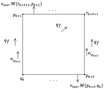
Figure 1: $\mathcal{M}(r_{k+\ell+1},q_{k})$ with orientations.

Our choice for the orientation of the relevant unstable submanifolds are

$$[U_{q_{k}}]=e_{k}\ldots e_{1}\,,\qquad\qquad\qquad [U_{p_{k+\ell}}]=e_{k+\ell+1}\ldots\widehat{e_{i_{p_{k+\ell}}}}\ldots e_{k}\ldots e_{1}\,,$$

$$[U_{p_{k+1}}]=e_{i_{p_{k+1}}}e_{k}\ldots e_{1}\,,\quad [U_{r_{k+\ell+1}}]=e_{k+\ell+1}\ldots e_{k}\ldots e_{1}\,.$$

Then by (A.3), $[\mathcal{M}(r,q)]=[U_{r}][U_{q}]^{-1}$, we find the orientations of the moduli spaces:

$$[\mathcal{M}(r_{k+\ell+1},q_{k})] =(e_{k+\ell+1}\ldots e_{k}\ldots e_{1})(e_{1}\ldots e_{k})=e_{k+\ell+1}\ldots e_{k+1}\,,$$ (A.7)

$$[\mathcal{M}(p_{k+\ell},q_{k})] =(e_{k+\ell+1}\ldots\widehat{e_{i_{p_{k+\ell}}}}\ldots e_{k}\ldots e_{1})(e_{1}\ldots e_{k})=e_{k+\ell+1}\ldots\widehat{e_{i_{p_{k+\ell}}}}\ldots e_{k+1}\,,$$

$$[\mathcal{M}(r_{k+\ell+1},p_{k+1})] =(e_{k+\ell+1}\ldots e_{k}\ldots e_{1})(e_{1}\ldots e_{k}e_{i_{p_{k+1}}})$$

$$=(-1)^{i_{p_{k+1}}-k-1}\,e_{k+\ell+1}\ldots\widehat{e_{i_{p_{k+1}}}}\ldots e_{k+1}\,.$$

And by (A.4), we also have

$$[\widetilde{\mathcal{M}}(r_{k+\ell+1},p_{k+\ell})] =[\mathcal{M}(r_{k+\ell+1},p_{k+\ell})][\nabla f]^{-1}$$

$$=(e_{k+\ell+1}\ldots e_{k}\ldots e_{1})(e_{1}\ldots e_{k}\ldots\widehat{e_{i_{p_{k+\ell}}}}\ldots e_{k+\ell+1})(e_{i_{p_{k+\ell}}})$$

$$=(-1)^{k+\ell+1-i_{p_{k+\ell}}}\,,$$

$$[\widetilde{\mathcal{M}}(p_{k+1},q_{k})] =[\mathcal{M}(p_{k+1},q_{k})][\nabla f]^{-1}$$

$$=(e_{i_{p_{k+1}}}e_{k}\ldots e_{1})(e_{1}\ldots e_{k})(e_{i_{p_{k+1}}})=1\,.$$

Hence, we find

$$[\mathcal{M}(p_{k+\ell},q_{k})\times\widetilde{\mathcal{M}}(r_{k+\ell+1},p_{k+\ell})] =(-1)^{k+\ell+1-i_{p_{k+\ell}}}\,e_{k+\ell+1}\ldots\widehat{e_{i_{p_{k+\ell}}}}\ldots e_{k+1}\,,$$ (A.8)

$$[\mathcal{M}(r_{k+\ell+1},p_{k+1})\times\widetilde{\mathcal{M}}(p_{k+1},q_{k})] =(-1)^{i_{p_{k+1}}-k-1}\,e_{k+\ell+1}\ldots\widehat{e_{i_{p_{k+1}}}}\ldots e_{k+1}\,.$$ (A.9)

Step 2: Orientation of the boundary components, $\mathcal{M}(p_{k+\ell},q_{k})\times\widetilde{\mathcal{M}}(r_{k+\ell+1},p_{k+\ell})$ and $\mathcal{M}(r_{k+\ell+1},p_{k+1})\times\widetilde{\mathcal{M}}(p_{k+1},q_{k})$, as specified by Stokes’ theorem.

For a manifold $N$ with boundary $\partial N$, Stokes’ theorem holds only if the orientation of the boundary $\partial N$ is chosen such that

$$[v_{out}][\partial N]=[N]$$ (A.10)

where $v_{out}$ is the outward pointing normal on the boundary.

For the boundary component $\mathcal{M}(p_{k+\ell},q_{k})\times\widetilde{\mathcal{M}}(r_{k+\ell+1},p_{k+\ell})$, the outward pointing normal at for instance $p_{k+\ell}$ can be expressed as (see Figure 1)

$$v_{out,\mathcal{M}(p_{k+\ell},q_{k})}=-e_{i_{p_{k+\ell}}}+\sum_{k+j\neq i_{p_{k+\ell}}}a_{j}e_{k+j}\,.$$

Therefore, the specified orientation from Stokes’ theorem (denoted with a subscript ‘$S$’) is

$$[\mathcal{M}(p_{k+\ell},q_{k})\times\widetilde{\mathcal{M}}(r_{k+\ell+1},p_{k+\ell})]_{S} =[v_{out,\mathcal{M}(p_{k+\ell},q_{k})}]^{-1}[\mathcal{M}(r_{k+\ell+1},q_{k})]$$

$$=(-e_{i_{p_{k+\ell}}})(e_{k+\ell+1}\ldots e_{k+1})$$

$$=(-1)^{k+\ell+i_{p_{k+\ell}}}\,e_{k+\ell+1}\ldots\widehat{e_{i_{p_{k+\ell}}}}\ldots e_{k+1}$$

$$=-[\mathcal{M}(p_{k+\ell},q_{k})\times\widetilde{\mathcal{M}}(r_{k+\ell+1},p_{k+\ell})]$$ (A.11)

having used (A.7) in the first line and (A.8) in the last line.

Similarly, for the boundary component $\mathcal{M}(r_{k+\ell+1},p_{k+1})\times\widetilde{\mathcal{M}}(p_{k+1},q_{k})$, the outward pointing normal at for instance $p_{k+1}$ can be expressed as (see Figure 1)

$$v_{out,\mathcal{M}(r_{k+\ell+1},p_{k+1})}=e_{i_{p_{k+1}}}+\sum_{k+j\neq i_{p_{k+1}}}a_{j}e_{k+j}\,.$$

This gives for the specified orientation from Stokes’ theorem

$$[\mathcal{M}(r_{k+\ell+1},p_{k+1})\times\widetilde{\mathcal{M}}(p_{k+1},q_{k})]_{S} =[v_{out,\mathcal{M}(r_{k+\ell+1},p_{k+1})}]^{-1}[\mathcal{M}(r_{k+\ell+1},q_{k})]$$

$$=(e_{i_{p_{k+1}}})(e_{k+\ell+1}\ldots e_{k+1})$$

$$=(-1)^{k+\ell+1-i_{p_{k+1}}}\,e_{k+\ell+1}\ldots\widehat{e_{i_{p_{k+1}}}}\ldots e_{k+1}$$

$$=(-1)^{\ell}[\mathcal{M}(r_{k+\ell+1},p_{k+1})\times\widetilde{\mathcal{M}}(p_{k+1},q_{k})]$$ (A.12)

having used (A.7) in the first line and (A.9) in the last line.

Finally, with (A.11)-(A.12) and matching up with the corresponding terms in (A.6), we have

$$c(d\psi)q_{k} =\sum_{r_{k+\ell+1}}\Bigg{[}-\sum_{p_{k+\ell}}\left(\int_{\overline{\mathcal{M}(p_{k+\ell},q_{k})}}\psi\right)n(r_{k+\ell+1},p_{k+\ell})$$

$$\qquad\qquad\qquad+\sum_{p_{k+1}}(-1)^{\ell}n(p_{k+1},q_{k})\left(\int_{\overline{\mathcal{M}(r_{k+\ell+1},p_{k+1})}}\psi\right)\Bigg{]}r_{k+\ell+1}$$

$$=-\partial c(\psi)q_{k}+(-1)^{\ell}c(\psi)\partial q_{k}$$

or equivalently, $-c(d\psi)=\partial c(\psi)+(-1)^{\ell+1}c(\psi)\partial$.

Department of Mathematics, University of California, Irvine, CA 92697, USA
Email address: dclausen@uci.edu

Department of Mathematics and Statistics, Washington University, St. Louis, MO 63130, USA
Email address: xtang@math.wustl.edu

Department of Mathematics, University of California, Irvine, CA 92697, USA
Email address: lstseng@math.uci.edu