ClawSAT: Towards Both Robust and Accurate Code Models

Abstract

We integrate contrastive learning (CL) with adversarial learning to co-optimize the robustness and accuracy of code models. Different from existing works, we show that code obfuscation, a standard code transformation operation, provides novel means to generate complementary ‘views’ of a code that enable us to achieve both robust and accurate code models. To the best of our knowledge, this is the first systematic study to explore and exploit the robustness and accuracy benefits of (multi-view) code obfuscations in code models. Specifically, we first adopt adversarial codes as robustness-promoting views in CL at the self-supervised pre-training phase. This yields improved robustness and transferability for downstream tasks. Next, at the supervised fine-tuning stage, we show that adversarial training with a proper temporally-staggered schedule of adversarial code generation can further improve robustness and accuracy of the pre-trained code model. Built on the above two modules, we develop ClawSAT, a novel self-supervised learning (SSL) framework for code by integrating CL with adversarial views (Claw) with staggered adversarial training (SAT). On evaluating three downstream tasks across Python and Java, we show that ClawSAT consistently yields the best robustness and accuracy (e.g. 11% in robustness and 6% in accuracy on the code summarization task in Python). We additionally demonstrate the effectiveness of adversarial learning in Claw by analyzing the characteristics of the loss landscape and interpretability of the pre-trained models. Codes are available at https://github.com/OPTML-Group/CLAW-SAT.

I Introduction

Recent progress in large language models for computer programs (i.e. code) suggests a growing interest in self-supervised learning (SSL) methods to learn code models–deep learning models that process and reason about code [1, 2, 3, 4, 5]. In these models, a task-agnostic encoder is learned in a pre-training step, typically on an unlabeled corpus. The encoder is appended to another predictive model which is then fine-tuned for a specific downstream task. In particular, contrastive learning (CL) based self-supervision [6, 7] has shown to improve the downstream performance of code reasoning tasks when compared to state-of-the-art task-specific supervised learning (SL) models [8, 9, 5].

While CL offers to be a promising SSL approach, nearly all the existing works focus on improving the accuracy of code models. Yet, some very recent works [10, 11, 12] showed that trained supervised code models are vulnerable to code obfuscation transformations. These works propose adversarial code–changing a given code via obfuscation transformations. Such transformed programs retain the functionality of the original program but can fool a trained model at test time. Figure 2 shows an example of adversarial code achieved by code obfuscation (more details in Section III). In software engineering, code obfuscation is a commonly-used method to hide code in software projects without altering their functionality [13, 14], and is consequently a popular choice among malware composers [15]. Thus, it is important to study how obfuscation-based adversarial code could affect code model representations learned by SSL. As an example, Schuster et al. [16] successfully demonstrate adversarial code attacks on a public code completion model pre-trained on GPT-2, a large language model of code.

Improving the robustness of ML models to adversarial code however comes at a cost–its accuracy (model generalization). Works in vision [17, 18] and text [19] have shown how adversarially trained models improve robustness at the cost of model accuracy. While some works [20, 21] provide a theoretical framework for how the robustness of learned models is always at odds with its accuracy, this argument is mainly confined to the SL paradigm and vision applications, and thus remains uninvestigated in SSL for code. While there exist similarities between SSL in vision and code, the discrete and structured nature of inputs, and the additional constraints enforced on views (obfuscated codes) introduce a new set of challenges that have been unexplored by the vision community.

I-A Overview of proposed approach

We offer two methods that help us improve not only the transfer of robustness from pre-trained models to downstream tasks, but also co-improve fine-tuned accuracy and robustness. The schematic overview of our proposal is shown in Figure 1. First, we propose a self-supervised pre-training method, contrastive learning with adversarial views (Claw), which leverages adversarially-obfuscating codes as positive views of CL so as to enforce the robustness of learned code representations. We formulate and achieve Claw through a bi-level optimization method. We show that the representations learned from these pre-trained models yield better robustness transfer to downstream tasks. Second, we propose staggered adversarial training (SAT) to preserve the robustness learned during pre-training while also learning task-specific generalization and robustness during fine-tuning. We show for the first time that the scheduler of adversarial code generation is adjustable and is a key to benefit both the generalization and robustness of code models.

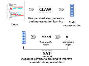
Figure 1: Schematic overview. We present Claw - a contrastive learning-based unsupervised method which learns adversarial views of the input code to in turn learn accurate and robust representations of the code. We also present SAT, a refinement to the adversarial training algorithm proposed by Madry et al. [22] which helps retain the task-independent robustness and accuracy learned by Claw while also learning task-specific accuracy and robustness. We show that ClawSAT yields better accuracy and robustness when compared to state-of-the-art self-supervised learning models for code.

I-B Contributions

On one hand, we propose Claw by extending the standard CL framework for code. As a baseline, we compare Claw to the state-of-the-art standard CL framework for code models - ContraCode released by [5]. We find Claw to ‘retain’ more robustness when compared to ContraCode. Further, we provide a detailed analysis of understanding this improved performance from the perspective of model interpretability and characteristics of its loss landscape. On the other hand, we integrate Claw with SAT to achieve the eventually fine-tuned ClawSAT models. We evaluate three tasks–code summarization, code completion, and code clone detection, in two programming languages - Python and Java, and two different decoder models–LSTMs and transformers. We show that ClawSAT outperforms ContraCode [5] by roughly $6\%$ on the summarization task, $2\%$ on the completion task, and $1\%$ on the code clone task in accuracy, and by $9\%$, $3\%$, and $1\%$ on robustness respectively. We study the effect of different attack strengths and attack transformations on this performance, and find it to be largely stable across different attack parameters.

II Related work

Due to a large body of literature on SSL and adversarial robustness, we focus our discussion on those relevant to code models and CL (contrastive learning).

II-A SSL for code

CL-based SSL methods offer a distinct advantage by being able to signal explicit examples where the representations of two codes are expected to be similar. While the method itself is agnostic to the input representation, all the works in CL for code models work on code tokens directly. Existing works [5, 23, 24, 25] show that CL models for code improve the generalization accuracy of fine-tuned models for different tasks when compared to other pre-training methods like masked language models. Each of these works uses semantics-preserving, random code transformations as positive views in its CL formulation. Such transformations help the pre-trained model learn the equivalence between representations of program elements which do not affect the executed output, such as the choice of variable names, the algorithmic ‘approach’ used to solve a problem, etc.

State-of-the-art CL-based representations generally provide an improvement in the range of $1\%$-$5\%$ points of F1/BLEU/accuracy scores when compared to their fully supervised counterparts and other pre-training methods like transformers, which is significant in the context of the code tasks they evaluate, providing clear evidence for the utility of SSL methods. While these methods improve the generalizability of task-specific models, none of these works have studied the robustness of these models, especially with a growing body of works showing the susceptibility of code models to adversarial attacks [12, 10, 11]. By contrast, the adversarial robustness of CL models for image classification has increasingly been studied by the vision community [26, 27, 28, 29]. These works have shown that CL has the potential to offer dual advantages of robustness and generalization. The fundamental differences in image and code processing, including how adversarial perturbations are defined in these two domains, motivate us to ask if and how the advantages offered by CL can be realized for code models.

II-B Adversarial robustness of code models: Attacks & defenses

[30, 31, 32, 33] showed that obfuscation transformations made to code can serve as adversarial attacks on code models. Following these works, recent papers [11, 10] proposed perturbing programs by replacing local variables and inserting print statements with replaceable string arguments. They found optimal replacements using a first-order optimization method, similar to HotFlip [34]. [12] framed the problem of attacking code models as a problem in combinatorial optimization, unifying the attempts made by prior works. [11, 10, 35] and [12] also proposed strategies to train code models against adversarial attacks. While [35] employed a novel formulation to decide if an input is adversarial, the other works employed the adversarial training strategy proposed by [18]. Recently,[36] proposed a black-box attack method to generate adversarial attacks for code, which is different from the white-box setting used in [30, 31, 32, 33]. In this paper, we only focused on the adversarial robustness of white-box attacks.

Work most relevant to ours. Our work comes closest to ContraCode, the system proposed by [5]. While they established the benefit of using CL-based unsupervised representation learning for code, the work neglects the interrelationship between pre-training and fine-tuning in the SSL paradigm, and the consequences of this relationship on both the robustness and generalization of the final model.

III Preliminaries

We begin by providing a brief background on code models, code obfuscation transformations, and SSL-aided predictive modeling for code. We then motivate the problem of how to advance SSL for code models. We study this through the lenses of accuracy and robustness of the learned models.

III-A Code and obfuscation transformations

Let $\mathcal{P}$ denote a computer program (i.e., code) which consists of a series of $n$ tokens $\{\mathcal{P}_{i}\}_{i=1}^{n}$ in the source code domain. For example, Figure 2 shows an example code $\mathcal{P}$. Given a vocabulary of tokens (denoted by $\Omega$), each token can be regarded as a one-hot vector of length $|\Omega|$. Here we ignore white spaces and other delimiters when tokenizing.

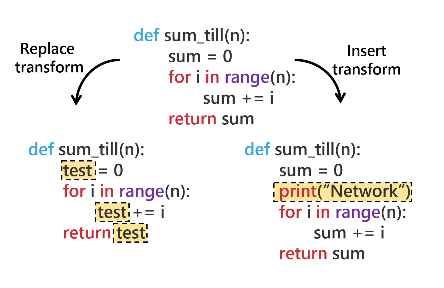
Figure 2: Two types of semantics-preserving transformations (obfuscations) can be made to a code to attack code models–replace - where existing code is modified at a site—location in the code, or insert - where new lines of code are inserted at a site. We select sites at random. The specific tokens used in these transformations (test and "Network" in the the example) can either be a random transformation $t_{\text{rand}}(\cdot)$–a randomly selected token from a pre-defined vocabulary, or can be an adversarial transformation $t_{\text{adv}}(\cdot)$, where the token is obtained from solving a first-order optimization designed to fool the model [12, 10, 11].

Let $t(\cdot)$ denote an obfuscation transformation, and $t(\mathcal{P})$ an obfuscated version of $\mathcal{P}$. $t(\mathcal{P})$ is semantically the same as $\mathcal{P}$ while possibly being different syntactically. Following the notations defined by [12] and [10], we refer to locations or tokens in a code which can be transformed as sites. We focus on replace and insert transformations, where either existing tokens in a source code are replaced by another token, or new lines of code are inserted in the existing code. For example, in Figure 2, the replace transformation modifies the variable sum with test, while the insert transformation introduces a new line of code print("Network").

Obfuscation transformations have been shown to serve as adversarial examples for code models (see Section II). During an adversarial attack, these transformations are made with the goal to get the resulting transformed code to successfully fool a model’s predictions. The transformations at any given site in a code, such as the tokens test, "Network" in Figure 2, can be obtained in two ways—by random transformations $t_{\text{rand}}(\cdot)$: they introduce a token sampled at random from $\Omega$, or through adversarial transformations $t_{\text{adv}}(\cdot)$: they solve a first-order optimization problem such that the transformed code maximizes the chances of the model making an incorrect prediction.

Our goal then turns to improve not only accuracy (i.e. prediction accuracy of properties of code $\mathcal{P}$) but also robustness (in terms of prediction accuracy of properties of $t(\mathcal{P})$, obfuscated transformations of $\mathcal{P}$).

III-B Problem statement

SSL typically includes two learning stages: self-supervised pre-training and supervised fine-tuning, where the former acquires deep representations of input data, and the latter uses these learned features to build a supervised predictor specific to a downstream task, e.g. code summarization [37] as considered in our experiments. In the pre-training phase, let $\boldsymbol{\theta}$ denote a feature-acquisition model (trained over unlabeled data), and $\ell(\boldsymbol{\theta})$ denote a pre-training loss, e.g. the normalized temperature-scaled cross-entropy (NT-Xent) loss used in CL [38, 6, 7]. In the supervised fine-tuning phase, let $\boldsymbol{\theta}_{\mathrm{ft}}$ denote the prediction head appended to the representation network $\boldsymbol{\theta}$, and $\ell_{\mathrm{ft}}(\boldsymbol{\theta}_{\mathrm{ft}}\circ\boldsymbol{\theta})$ denote a task-specific fine-tuning loss seen as a function of the entire model $\boldsymbol{\theta}_{\mathrm{ft}}\circ\boldsymbol{\theta}$, where $\circ$ denotes model composition. Fine-tuning is performed over labeled data. The SSL pipeline can then be summarized as

$$\begin{array}[]{rl}\text{Pre-training:}&\boldsymbol{\theta}_{\mathrm{pre}}=\displaystyle\arg\min_{\boldsymbol{\theta}}~{}\ell(\boldsymbol{\theta}),\\ \text{(Full) Fine-tuning:}&\displaystyle\operatorname*{\text{minimize}}_{\boldsymbol{\theta}_{\mathrm{ft}},\boldsymbol{\theta}}~{}\ell_{\mathrm{ft}}(\boldsymbol{\theta}_{\mathrm{ft}}\circ\boldsymbol{\theta}),{}\\ &\text{with initialization $\boldsymbol{\theta}=\boldsymbol{\theta}_{\mathrm{pre}}$}.\end{array}$$ (4)

We remark that if we fix $\boldsymbol{\theta}=\boldsymbol{\theta}_{\mathrm{pre}}$ in (4) during fine-tuning, then the resulting scheme is called partial fine-tuning (PF), which only learns the prediction head $\boldsymbol{\theta}_{\mathrm{ft}}$. Based on (4) for code, this work tackles the following research questions:

IV Method

In this section, we will study the above (Q1)-(Q2) in-depth. To address (Q1), we will develop a new pre-training method, termed Claw, which integrates CL with adversarial views of codes. The rationale is that promoting the invariance of representations to possible adversarial candidates should then likely improve the robustness of models fine-tuned on these representations. To answer (Q2), we will a novel fine-tuning method, termed staggered adversarial training (SAT), which can balance the supervised fine-tuning with unsupervised pre-training. The rationale is that the supervised fine-tuning overrides pre-trained data representations and hardly retains the robustness and generalization benefits achieved during pre-training. We will show that the interplay between pre-training and fine-tuning should be carefully studied for robustness-generalization co-improvement in SSL for code.

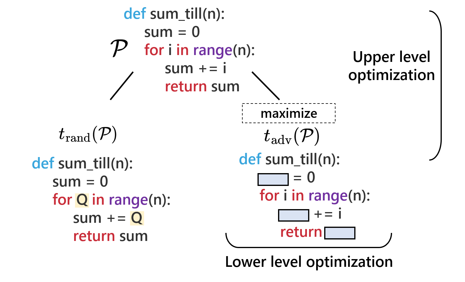
Figure 3: During pre-training, we propose Claw containing two optimization problems: (1) to learn invariant code representations by minimizing the representation distances of a code ($\mathcal{P}$) from all its views ($t_{\text{rand}}(\mathcal{P})$, $t_{\text{adv}}(\mathcal{P})$) via CL, and (2) to generate an adversarial code $t_{\text{adv}}(\mathcal{P})$ (‘hard’ positive example) by maximizing its representation distance from $\mathcal{P}$. In the example, this requires solving for a replacement token at the randomly selected site marked as •.

IV-A Claw: CL with adversarial codes

CL [6, 7] proposes to first construct ‘positive’ example pairs (i.e., original data paired with its transformations or ‘views’), and then maximize agreement between them while contrasting with the rest of the data (termed ‘negatives’). In programming languages, code obfuscation transformations naturally serve as view generators of an input code. While we reuse the same set of transformations (that are applicable to Python and Java programs) employed by the prior work [5], we generate transformed views of the code differently. [5] use random views in their CL setup, which select and apply a transformation at random from the set of permissible transformations. We generate worst-case, optimization-based adversarial codes [10, 12] resulting in ‘adversarial views’.

Infusing the original code, its random view, and its adversarial view into CL, we obtain a three-view positive tuple, denoted by ($\mathcal{P}$, $t_{\text{rand}}(\mathcal{P})$, $t_{\text{adv}}(\mathcal{P})$). Since the generation of adversarial code (the right tokens for a given site) is in itself an additional optimization task, we leverage a bi-level optimization (BLO) framework [39, 40] and define optimization problems at two levels: the upper-level problem aims to solve the multi-view CL, while the lower-level problem aims to solve adversarial code generation (see an illustration in Figure 3). This results in the following formulation for our proposed approach Claw:

$$\begin{array}[]{l}\displaystyle\operatorname*{\text{minimize}}_{\boldsymbol{\theta}}~{}\mathbb{E}_{\mathcal{P},t_{\text{rand}}}[\ell_{\mathrm{NT-Xent}}(\boldsymbol{\theta};\mathcal{P},t_{\text{rand}}(\mathcal{P}))]+\\ \hskip 45.5244pt\underbrace{\mathbb{E}_{\mathcal{P}}[\ell_{\mathrm{NT-Xent}}(\boldsymbol{\theta};t_{\text{rand}}(\mathcal{P}),t_{\text{adv}}(\mathcal{P}))]}_{\text{Upper level: Multi-view CL}}\vspace*{1mm}\\ \operatorname*{\text{subject to}}~{}t_{\text{adv}}(\mathcal{P})=\underbrace{\displaystyle\arg\max_{\mathcal{P}^{\prime}}\ell_{\mathrm{NT-Xent}}(\boldsymbol{\theta};\mathcal{P},\mathcal{P}^{\prime})}_{\text{Lower level: Adversarial code generation}},\end{array}$$ (8)

where the three-view objective function is constructed by NT-Xent losses applied to two positive pairs $(\mathcal{P},t_{\text{rand}}(\mathcal{P}))$ and $(t_{\text{rand}}(\mathcal{P}),t_{\text{adv}}(\mathcal{P}))$, respectively. The first positive pair is to gain the generalizable code representation by promoting the representation invariance across the original view $\mathcal{P}$ and its (benign) randomly-obfuscating view $t_{\text{rand}}$, as suggested in [5]. The second positive pair is to enforce the adversary-resilient code representation by promoting the representation invariance across the benign code $t_{\text{rand}}$ and the adversarial code $t_{\text{adv}}(\mathcal{P})$. Given two codes $\mathcal{P}_{1}$ and $\mathcal{P}_{2}$, the specific form of $\ell_{\mathrm{NT-Xent}}$ is given by as follows:

$$\begin{array}[]{l}\ell_{\mathrm{NT-Xent}}=-\frac{1}{2}\sum_{i=1}^{2}\log\frac{\exp\big{(}\text{sim}(\mathbf{z}_{1}(\boldsymbol{\theta}),\mathbf{z}_{2}(\boldsymbol{\theta}))/t\big{)}}{\sum_{k\in\mathcal{N}(i)},\exp\big{(}\text{sim}(\mathbf{z}_{i}(\boldsymbol{\theta}),\mathbf{z}_{k}(\boldsymbol{\theta}))/t\big{)}}\end{array}$$ (10)

where $\mathbf{z}_{i}$ denotes the feature representation of the input code $\mathcal{P}_{i}$ achieved through the representation network $\boldsymbol{\theta}$, $\mathrm{sim}(\mathbf{z}_{i},\mathbf{z}_{j})$ denotes the cosine similarity between two feature representations $\mathbf{z}_{i}$ and $\mathbf{z}_{j}$, $t>0$ is a temperature parameter, and $\mathcal{N}(i)$ is the set of batch data except the data sample $i$ [6].

To solve the BLO problem (8), we apply an alternating optimization method [41, 39]. Specifically, by fixing the representation network $\boldsymbol{\theta}$, the lower-level adversarial code generation is accomplished using first-order gradient descent following [12, 10]. Given the generated adversarial code $t_{\mathrm{adv}}(\mathcal{P})$, we then in turn solve the upper-level CL problem. The above procedure is alternatively executed for every data batch.

Adversarial view is beneficial to representation learning. To highlight the effectiveness of incorporating adversarial codes in CL at the pre-training phase, the rows ‘ContraCode-PF’ and ‘Claw-PF’ of Table I demonstrate a warm-up experiment by comparing the performance of the proposed pre-training method Claw with that of the baseline approach ContraCode [5]. To precisely characterize the effect of the learned representations on code model generalization and robustness, we partially fine-tune (PF) a seq2seq model on the downstream task of summarizing code (details in Section V) in Python (SummaryPy) and Java (SummaryJava) by fixing the set of weights learned during pre-training. Gen-F1 and Rob-F1 are the generalization F1-scores and the robust F1-scores, i.e., F1 scores of the model when attacked with adversarial codes. Partially fine-tuning these models allows us to study the sole contribution of the pre-training method in the learned robustness and generalization of the model. As we can see, the partially fine-tuned Claw model (termed Claw-PF) outperforms the baseline ContraCode-PF, evidenced by the substantial robustness improvement (4.38% increase in Rob-F1 in SummaryPy) as well as lossless or better generalization performance (1.58% increase in Gen-F1 scores on SummaryJava). It is worth noting that adversarial codes serve as ‘hard’ positive examples in the representation space (given by maximizing the representation distance between $\mathcal{P}$ and its perturbed variant $\mathcal{P}^{\prime}$ in the lower optimization level of Claw, (8)). The benefit of hard positive examples in improving generalization has also been seen in vision [42, 43, 44].

Model	Partial fine-tuning
	SummaryPy		SummaryJava
	Gen-F1	Rob-F1	Gen-F1	Rob-F1
ContraCode-PF	25.46	15.47	20.92	16.63
Claw-PF	25.45	19.05	22.50	17.14
	Full fine-tuning
ContraCode-ST	36.28	28.97	41.37	33.01
Claw-ST	36.57	29.97	41.23	32.53
ContraCode-AT	32.80	32.39	38.67	35.91
Claw-AT	32.97	32.65	38.86	36.10

TABLE I: Partially fine-tuned (PF) models show that Claw improves robustness. Standard training (ST) yields better generalization than adversarial training (AT) while the latter provides better robustness.

IV-B SAT: Staggered adversarial training for fine-tuning

As shown in the previous section, an appropriate pre-training method can improve the quality of learned deep representations, which help improve the robustness and accuracy of a code model. However, the state of the model present at the end of the pre-training phase may no longer hold after supervised fine-tuning. That is because supervised learning (trained on labeled data vs. unlabeled data in representation learning) may significantly alter the characteristics of the learned representations. Thus, a desirable fine-tuning scheme should be able to yield accuracy and robustness improvements complementary to the representation benefits provided by pre-training. Towards this goal, we posit that fine-tuning should not be designed in a way which merely optimizes a single performance metric–either accuracy or robustness.

To justify this hypothesis, we consider two extreme cases during fine-tuning: (i) standard training (ST)-based FF, and (ii) adversarial training (AT)-based FF [18]. ST is essentially the same setup as fully supervised training with the only difference being in the set of initial parameters of the model. This setup optimizes improving a model’s generalization ability. On the other hand, AT optimizes improving the model’s adversarial robustness.

The last four rows of Table I present the performance of these two extreme fine-tuning cases applied to the pre-trained models provided by ContraCode [5] and Claw, respectively. As we can see, when either ST or AT is used, different pre-training methods (ContraCode and Claw) lead to nearly the same generalization and robustness performance. This shows that fine-tuning, when aggressively optimizing one particular performance metric, could override the benefits achieved during pre-training. To this end, we propose staggered AT (SAT), a hybrid of ST and AT by adjusting the time instances (in terms of epoch numbers) at which adversarial codes are generated (see Algorithm LABEL:alg:sat). [8figures_tables.tex]alg:sat SAT involves two key steps—training a model $\mathcal{M}\mathrel{\mathop{:}}=\{\boldsymbol{\theta},\boldsymbol{\theta}_{\mathrm{ft}}\}$ on a batch $\mathcal{B}$ of data (step 1), and attacking the learned model at a staggered frequency $\tau$ (steps 2-3). Different from AT, adversarial code is not generated in every data batch. Instead, in SAT, we propose reducing the frequency of adversarial learning. Accordingly, adversarial code generation occurs at the frequency of each epoch or at every few epochs. This ensures the model parameters retain as much of the attributes from pre-training while also learning task-specific generalization and robustness. In SAT, the model is finetuned using ($\mathcal{B}_{i}$ + $\mathcal{B}^{\prime}_{i}$) where $\mathcal{B}_{i}^{\prime}$ refers to the generated adversarial code corresponding to $\mathcal{B}_{i}$. Eventually, by combining the proposed pre-training scheme Claw with the fine-tuning scheme SAT, we term the resulting SSL framework for code as ClawSAT.

V Experiment Setup

We describe the following aspects of our experiment setup - the task, dataset, and the details of the model.

[8figures_tables.tex]tab:generalization-robustness

Task, dataset, error metrics. We evaluate our algorithm on four tasks: (1) code summarization [37, 45, 46, 47, 48, 5] in Python, (2) code summarization in Java (generates English description for given code snippet), (3) code completion in Python [49] (generates the next six tokens for a given code snippet), and (4) code clone detection [50] in Java (classifies whether a pair of code snippets are clones of each other). For models evaluated in Python, we pre-train on the Py-CSN dataset [51], containing $\sim$ $500$K methods, and fine-tune on the Py150 dataset [52], containing $\sim$ $200$K methods. For Java, we pre-train on the Java-CSN dataset [51] containing $\sim$ $600$K and fine-tune on the Java-C2S [37] dataset containing $\sim$ $500$K methods. We use the F1-score $\in[0,100]$ to measure the performance of all our models, consistent with all the related works, including [5]. A higher value indicates that the model generalizes better to the task. While these F1-scores are correlated to BLEU scores, they directly account for token-wise mis-predictions. The F1 scores are computed following [53, 54] Specifically, for each of our models, we reuse the two F1 scores: Gen-F1 - the model’s generalization performance on a task, and Rob-F1 - the model’s performance on the task when semantics-preserving, adversarially-transformed obfuscated codes are input to it; see details below.

Adversarial attacks, attack strength, code transformations. When attacking code models, we use the formulation by [12] to define the strength of an attack. Specifically, selecting a larger number of sites in a code—locations or tokens in a code which can be transformed to produce an adversarial outcome—corresponds to a stronger adversarial attack, since this allows multiple changes to be made to the code. Also, we follow [12, 10] to specify the set of code transformations: replace (renaming local variables, renaming function parameters, renaming object fields, replacing boolean literals) and insert (inserting print statements, adding dead code).

In our setup, we can leverage the attack strength at three stages–during pre-training (using adversarially attacked code as views), when fine-tuning with adversarial training AT [18] or SAT, and when evaluating robustness on an unseen test set. Unless specified otherwise, we pre-train on one site, attack one site in each iteration of SAT, and attack one site during evaluation. In Table LABEL:tab:sensitivity ,we analyze the effect of varying the number of sites at each of these stages. We apply the first-order optimization method proposed in [10] to generate adversarial codes. To adversarially train these models during fine-tuning, we employ either AT [18] or our proposed SAT for code.

Baselines. We compare ClawSAT to three baselines. (1) A supervised model (model M₁ in Table LABEL:tab:generalization-robustness) - Pre-training has no effect on a fully supervised model. (2) Adversarially trained supervised model (M₂) on top of ${{M}\textsubscript{1}}$ - we use the AT setup first proposed by [10], which in turn employs the setup from [18]. Due to the characteristics of AT, we expect to see an improvement in its Rob-F1 as compared to M₁ but a decrease in Gen-F1. (3) The ContraCode model (M₃) from [5]. ContraCode reflects the state-of-the-art in pre-training methods as it outperforms other pre-training models like BERT-based models and GPT3-Codex. Hence, we do not compare ourselves again to other pre-training models.

Models. For the summarization and completion tasks, we experiment with two seq2seq architectures–LSTMs and transformers. For the detection task, we use a fully connected linear layer as a decoder. The decoders are trained to predict the task (generating English sentence summaries, generating code completions, flagging code clones respectively) in both the fine-tuned and standard training settings. When fine-tuning, we use the learned encoders from the pre-trained models. For the summarization and completion tasks, we report all our results on the LSTM decoder (Table LABEL:tab:generalization-robustness), and compare the performance of transformers in our ablation study. The LSTM encoder has 2 layers across all experiments. In the code summarization tasks, there exists another two-layer decoder added to the encoder to generate the summary of the programming language. In the code completion task, we also add a two-layer decoder to generate the code snippets. In the code clone detection task, we add one linear layer to map the data representations to the data labels. As for the transformer architecture, The transformer encoder has 6 layers and the transformer decoder has another 6 layers to generate the programming language summary.

Hyperparameter setup. We optimize model parameters using Adam with linear learning rate warm-up. For the bidirectional LSTM encoders, the maximum learning rate for ContraCode and Claw is $10^{-4}$, and then is decayed accordingly. For the transformer-type encoder, the maximum learning rate is $10^{-4}$ for ContraCode and $10^{-5}$ for Claw. For different downstream tasks, we optimize the parameters using Adam with step-wise learning rate decay. The maximum learning rates of ST, AT, SAT are $10^{-3}$ on code summarization and code completion tasks, and $10^{-4}$ for code clone detection tasks. For downstream tasks using transformer, the learning rates of ST, AT, SAT are $10^{-4}$. All of the downstream tasks are finetuned for 10 epochs with practical convergence, and we utilize a validation dataset to pick the best-performed model. All of the experiments are conducted on 4 Tesla V100 GPU with 16 GB memory.

VI Experiment Results

We summarize the overall performance of ClawSAT and follow that up with multiple additional analyses and ablations to better understand our model’s performance.

VI-A Overall performance

We evaluate the different pre-training and fine-tuning strategies we consider in Section IV. The accuracy and robustness F1-scores of the different models are shown in Table LABEL:tab:generalization-robustness. Models M₁-M₃ are the baselines described in the previous section. Model M₄ pertains to using a Claw encoder with standard training (ST) for the downstream task. Model M₅ pertains to using a Claw encoder with standard adversarial training (AT) for the downstream task. And finally, M₆ pertains to using SAT for the downstream task with a Claw encoder. We observe the following:

First, from the perspective of accuracy, Table LABEL:tab:generalization-robustness shows that our proposal ClawSAT (model M₆) outperforms all the baselines on Gen-F1. Particularly, ClawSAT achieves nearly 8% accuracy improvement over ContraCode (M₃) on SummaryPy. Second, we see that ClawSAT can substantially help improve the robustness (measured by Rob-F1) of a downstream model. Compared to M₃, we see an improvement of $14.7\%$ for SummaryPy, and $5.8\%$ for SummaryJava. Similarly, the gain in robustness is much more substantial in CompletePy than in accuracy. CloneJava is the simplest of the four tasks, and we see comparable accuracies across all the models we evaluate. Additionally, we adversarially train baselines as well (models M₂ and M₅ respectively) and compare their robustness scores to ours (M₆). We make two observations– (a) As is expected with AT, we notice a drop in these models’ accuracy–the Gen-F1 scores of M₅ is lower than that of its standard-training counterpart M₄ (the same trend is observed between M₂ and M₁ as well). (b) While AT-based fine-tuning provides an expected improvement in robustness over the other baselines that use ST-based fine-tuning, the Rob-F1 they achieve is still much lower than our model. This is because the robustness gain at the pre-training phase was overridden by AT at the fine-tuning phase.

In what follows, we analyze the performance of Claw and SAT separately from different perspectives.

VI-B Why is Claw effective? A model landscape perspective

[8figures_tables.tex]lossclaw

⬇ def _makeOne(self,discriminator=None ,family=None): from ..index import AllowedIndex index = AllowedIndex(discriminator,family=family) return index ⬇ def _makeOne(self,repeat=None ,family=None): from ..index import AllowedIndex index = AllowedIndex(repeat,family=family) return index (a) Sample (b) Adversarially perturbed version of sample (a1) ⬇ def _makeOne(self,discriminator=None family=None,action_Mode=None): from ..indexes import FieldIndex return FieldIndex(discriminator,family,action_mode) ⬇ def _makeOne(self,discriminator=None family=None,action_Mode=None): from ..indexes import FieldIndex return FieldIndex(discriminator,family,action_mode) (c) EBE similar to (a) - Claw (d) EBE similar to (a) - ContraCode ⬇ def _makeOne(self,discriminator=None family=None,action_Mode=None): from ..indexes import FieldIndex return FieldIndex(discriminator,family,action_mode) ⬇ def buildIndex(self,l): index = self.mIndex() for strat, end, value in self.l: index.add(strat,end) return index (e) EBE similar to (b) - Claw (f) EBE similar to (b) - ContraCode

Figure 4: Explanation-by-example to demonstrate the robustness benefits of Claw. (a) Sample program from the test set (b) Adversarially perturbed variant of the sample program. (c-d) Examples closest to the sample program (a) when using Claw and ContraCode. (e-f) Examples closest to the perturbed variant (b) when using Claw and ContraCode.

Liu et. al.[55] show that the generalization benefit of an approach in the‘pre-training + fine-tuning’ paradigm can be deduced by the flatness of the loss landscape of the pre-trained model. This would then let fine-tuning to force the optimization for fine-tuning to stay in a certain neighborhood of the pre-trained model of high quality.

To plot the loss landscapes, we follow the procedure from Li et. al.[56] by plotting

$$f(\alpha,\beta)=\ell(\theta^{\star}+\alpha\delta+\beta\eta)$$ (11)

where $\delta$ and $\eta$ are two random direction vectors in the parameters’ subspace, and $\theta^{\star}$ is the parameters of a model. We average the supervised loss from the partially fine-tuned models from $640$ randomly selected samples in our test set (out of $10000$, $6.4\%$).

Next, we show another way to justify the flatness merit of Claw’s loss landscape. The key idea is to track the deviations of the weights of the pre-trained encoders in the fine-tuned setting, as inspired by [55]. Specifically, let $\boldsymbol{\theta}_{\mathrm{pre}}$ and $\boldsymbol{\theta}_{\mathrm{pre}}^{\prime}$ denote the weights of the representation model $\boldsymbol{\theta}$ pre-trained by Claw and the fine-tuned weights obtained by using different fine-tuning methods, respectively. It was shown in [55] that the generalization benefit of an approach in the‘pre-training + fine-tuning’ paradigm can be deduced by the deviation between the fine-tuned weights $\boldsymbol{\theta}_{\mathrm{pre}}^{\prime}$ and the pre-trained weights $\boldsymbol{\theta}_{\mathrm{pre}}$. This would then let fine-tuning to force the optimization of $\boldsymbol{\theta}_{\mathrm{pre}}^{\prime}$ to stay in a certain neighborhood of $\boldsymbol{\theta}_{\mathrm{pre}}$. We have already shown that Claw will lead to a flatter loss landscape compared to ContraCodepreviously. Here we computed the Frobenius norm $||\boldsymbol{\theta}_{\mathrm{pre}}^{\prime}-\boldsymbol{\theta}_{\mathrm{pre}}||_{\mathrm{F}}$ as a proxy to justify the generalization benefit following [55].

[8figures_tables.tex]tab:weights-epoch-model

Table LABEL:tab:weights-epoch-model summarizes the aforementioned weight characteristics for the code summarization task. As we can see, the weight deviation corresponding to Claw is less than that associated with ContraCode given a finetuning method.

VI-C Interpretability of learned code representations

We evaluate the robustness benefit of Claw through the lens of (input-level) model explanation. Following the observations from Jeyakumar et. al.[57] on probing models locally, we investigate Claw and ContraCode using a training data-based model explanation method: explanation-by-example (EBE) [58]. The core idea is to leverage train-time data to explain test-time data by matching their respective representations. If the pre-trained models are robust, adversarially perturbing the samples should not alter their representations and thus should be mapped to the same set of closest training examples that were found without perturbations.

In what follows, we peer into the EBE method’s results with an example below.

$\bullet$ A sample program from the test-set:

⬇

def __init__(self,helper_name):

self.helper_name = helper_name

self.cheeks = []

$\bullet$ Adversarially perturbed variant of the sample program: The adversarial attack algorithm replaces the method argument helper with edges.

⬇

def __init__(self,edges):

self.helper_name = edges

self.cheeks = []

$\bullet$ EBE sample in the train-set closest to the sample program when using ContraCode or Claw: This is the example whose ContraCode or Claw representation (encoder trained by ContraCode or Claw) is closest to the representation of the sample program. We can find that they have the same functionality.

⬇

def __init__(self,name):

self.name = name

self.warning = []

$\bullet$ EBE sample in the train-set closest to the perturbed variants of sample program from ContraCode: We can observe that the closest program of the perturbed program in the training dataset is different from that of the original program. The new closest program has different functionality from the previous test sample program.

⬇

def setUp(self):

super(ApiCallHandlerRegressionTest,self).setUp()

self.checks = []

$\bullet$ EBE sample in the training-set closest to the perturbed sample program from Claw: This example pertains to the representation that is closest to the representation of the sample program computed by an encoder trained by Claw. We see that despite comparing it to a perturbed sample’s representation, the example found by EBE corresponds to the unpertrubed sample program, suggesting the robustness of Claw over ContraCode.

⬇

def __init__(self,name):

self.name = name

self.warning = []

We also provide more examples in Figure 4. Figure 4.a shows a sample Python program and Figure 4.b shows its respective adversarially perturbed variant. The closest training programs in the training set mapped to the representations before perturbations are shown in Figures 4.c and 4.d; and those mapped to the representations after perturbations are shown in Figures 4.e and 4.f.

VI-D SAT enables generalization-robustness sweet spot

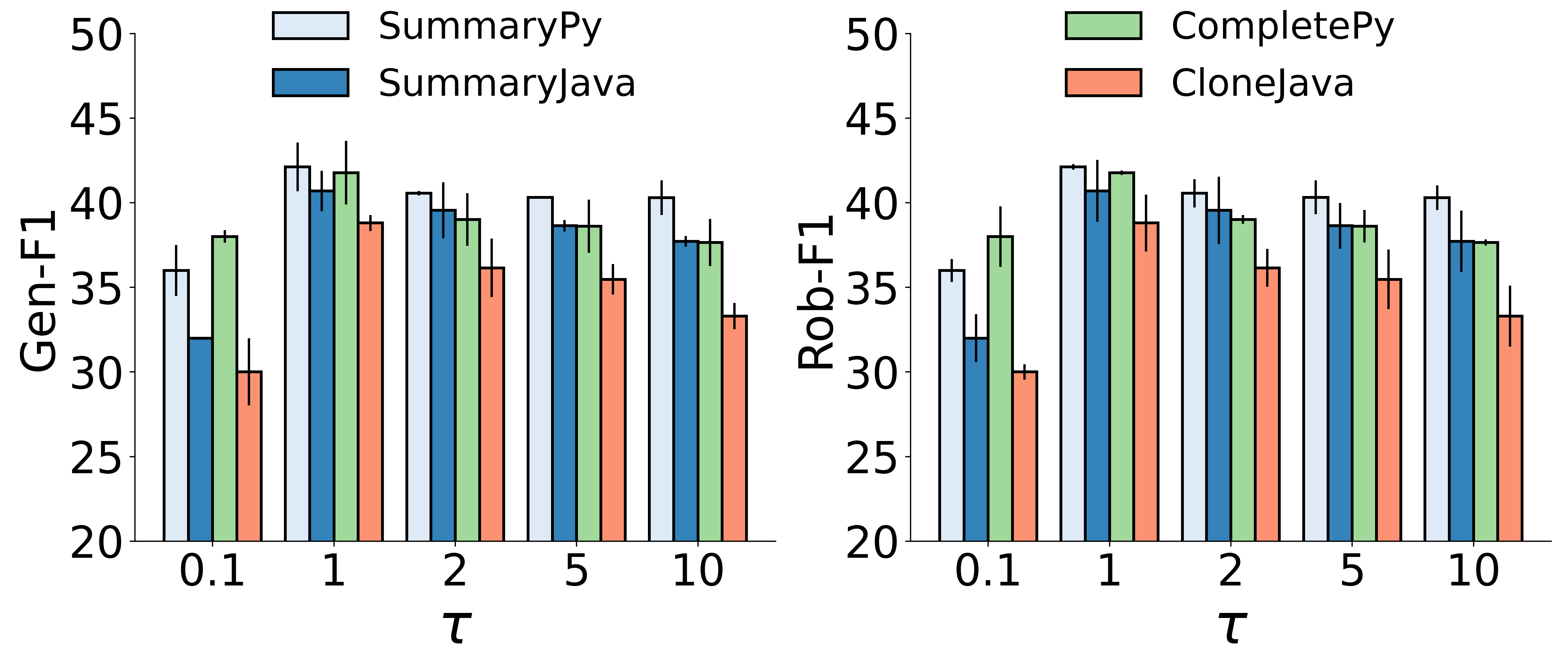
Figure 5: Effect of different update schedules ($\tau$, see Algorithm LABEL:alg:sat) on Gen-F1 and Rob-F1.

Figure 5.(A) shows the results from our experiments on the code summarization task where we vary $\tau$, the frequency of attacking the code model during SAT (see Algorithm LABEL:alg:sat).

We generate adversarial code tokens every $\tau^{\text{th}}$ epoch, where we vary $\tau$ from less than $1$ (corresponds to an update occurring at every batch within an epoch; this is the AT algorithm from [18]) to $10$. The X-axis shows this frequency. We plot both Gen-F1 (left) and Rob-F1 (right) of the adversarially trained model when varying $n$. Across the four tasks we evaluate in this work, We find that a sweet spot exists in a less frequent epoch-wise schedule, associated with ClawSAT (M₆, which corresponds to $\tau=1$), which improves both Gen-F1 and Rob-F1 over M₅ (which corresponds to $\tau=0.1$).

VI-E ClawSAT on a different architecture

[8figures_tables.tex]tab:transformer We further evaluate SAT on a different model architecture. We consider the transformer architecture (6-layer encoder and 6-layer decoder following [5]), and observe similar results (see Table LABEL:tab:transformer): ClawSAT offers the best accuracy and robustness.

VI-F Extended study to integrate SAT with ContraCode

[8figures_tables.tex]tab:generalization-robustness2 To further verify the effectiveness of SAT, we employ it in ContraCode—we modify their implementation to introduce a staggered adversarial training schedule. Table LABEL:tab:generalization-robustness2 tabulates its performance. We find that SAT also benefits ContraCode, but the gain is smaller than ClawSAT (M₆, Table LABEL:tab:generalization-robustness). This justifies the complementary benefits of Claw and SAT.

VI-G Sensitivity of SAT to code transformation and attack strength types.

[8figures_tables.tex]tab:sensitivity We evaluate the sensitivity of our best-performing model on differing attack conditions. We consider two factors: (1) Transformation type: we study the effect of the two transformation types–replace and insert, and their combination. (2) Attack strength: we vary the number of sites—locations in the codes that can be adversarially transformed.

We summarize our results in Table LABEL:tab:sensitivity. The values a, b in each cell correspond to Gen-F1 and Rob-F1 of ClawSAT respectively.

VII Conclusion & Discussion

In this work, we aim to achieve the twin goals of improved robustness and generalization in SSL for code, specifically in contrastive learning. We realize this by proposing two improvements–adversarial positive views in contrastive learning, and a staggered AT schedule during fine-tuning. We find that each of these proposals provides substantial improvements in both the generalization and robustness of downstream models; their combination, ClawSAT, provides the best overall performance. Given the growing adoption of SSL-based models for code-related tasks, we believe our work lays out a framework to gain a principled understanding into the working of these models. Future works should study this problem while attempting to also establish a theoretically sound foundation.

When compared to SSL for vision, it seems SSL for codes benefits from milder adversarial training during fine-tuning. Stronger attack methods for code might be needed to explore this phenomenon further. It will also be beneficial to understand how code models respond to perturbations, and to contrast it to our understanding of continuous data perturbations in vision.

References

- [1] A. Kanade, P. Maniatis, G. Balakrishnan, and K. Shi, “Learning and evaluating contextual embedding of source code,” in International Conference on Machine Learning. PMLR, 2020, pp. 5110–5121.
- [2] M. Chen, J. Tworek, H. Jun, Q. Yuan, H. P. de Oliveira Pinto, J. Kaplan, H. Edwards, Y. Burda, N. Joseph, G. Brockman, A. Ray, R. Puri, G. Krueger, M. Petrov, H. Khlaaf, G. Sastry, P. Mishkin, B. Chan, S. Gray, N. Ryder, M. Pavlov, A. Power, L. Kaiser, M. Bavarian, C. Winter, P. Tillet, F. P. Such, D. Cummings, M. Plappert, F. Chantzis, E. Barnes, A. Herbert-Voss, W. H. Guss, A. Nichol, A. Paino, N. Tezak, J. Tang, I. Babuschkin, S. Balaji, S. Jain, W. Saunders, C. Hesse, A. N. Carr, J. Leike, J. Achiam, V. Misra, E. Morikawa, A. Radford, M. Knight, M. Brundage, M. Murati, K. Mayer, P. Welinder, B. McGrew, D. Amodei, S. McCandlish, I. Sutskever, and W. Zaremba, “Evaluating large language models trained on code,” 2021.
- [3] Z. Chen, V. J. Hellendoorn, P. Lamblin, P. Maniatis, P.-A. Manzagol, D. Tarlow, and S. Moitra, “PLUR: A unifying, graph-based view of program learning, understanding, and repair,” in Advances in Neural Information Processing Systems, A. Beygelzimer, Y. Dauphin, P. Liang, and J. W. Vaughan, Eds., 2021. [Online]. Available: https://openreview.net/forum?id=GEm4o9A6Jfb
- [4] N. Jain, S. Vaidyanath, A. S. Iyer, N. Natarajan, S. Parthasarathy, S. K. Rajamani, and R. Sharma, “Jigsaw: Large language models meet program synthesis,” CoRR, vol. abs/2112.02969, 2021. [Online]. Available: https://arxiv.org/abs/2112.02969
- [5] P. Jain, A. Jain, T. Zhang, P. Abbeel, J. Gonzalez, and I. Stoica, “Contrastive code representation learning,” in Proceedings of the 2021 Conference on Empirical Methods in Natural Language Processing. Online and Punta Cana, Dominican Republic: Association for Computational Linguistics, Nov. 2021, pp. 5954–5971. [Online]. Available: https://aclanthology.org/2021.emnlp-main.482
- [6] T. Chen, S. Kornblith, M. Norouzi, and G. Hinton, “A simple framework for contrastive learning of visual representations,” in International conference on machine learning. PMLR, 2020, pp. 1597–1607.
- [7] K. He, H. Fan, Y. Wu, S. Xie, and R. Girshick, “Momentum contrast for unsupervised visual representation learning,” in Proceedings of the IEEE/CVF Conference on Computer Vision and Pattern Recognition, 2020, pp. 9729–9738.
- [8] N. D. Bui, Y. Yu, and L. Jiang, “Self-supervised contrastive learning for code retrieval and summarization via semantic-preserving transformations,” in Proceedings of the 44th International ACM SIGIR Conference on Research and Development in Information Retrieval, 2021, pp. 511–521.
- [9] Y. Ding, L. Buratti, S. Pujar, A. Morari, B. Ray, and S. Chakraborty, “Contrastive learning for source code with structural and functional properties,” CoRR, vol. abs/2110.03868, 2021. [Online]. Available: https://arxiv.org/abs/2110.03868
- [10] J. Henkel, G. Ramakrishnan, Z. Wang, A. Albarghouthi, S. Jha, and T. Reps, “Semantic robustness of models of source code,” in 2022 IEEE International Conference on Software Analysis, Evolution and Reengineering (SANER), 2022, pp. 526–537.
- [11] N. Yefet, U. Alon, and E. Yahav, “Adversarial examples for models of code,” Proceedings of the ACM on Programming Languages, vol. 4, no. OOPSLA, pp. 1–30, 2020.
- [12] S. Srikant, S. Liu, T. Mitrovska, S. Chang, Q. Fan, G. Zhang, and U. O’Reilly, “Generating adversarial computer programs using optimized obfuscations,” in International Conference on Learning Representations, 2021. [Online]. Available: https://openreview.net/forum?id=PH5PH9ZO_4
- [13] C. S. Collberg and C. Thomborson, “Watermarking, tamper-proofing, and obfuscation-tools for software protection,” IEEE Transactions on software engineering, vol. 28, no. 8, pp. 735–746, 2002.
- [14] C. Linn and S. Debray, “Obfuscation of executable code to improve resistance to static disassembly,” in Proceedings of the 10th ACM conference on Computer and communications security, 2003, pp. 290–299.
- [15] S. Schrittwieser, S. Katzenbeisser, J. Kinder, G. Merzdovnik, and E. Weippl, “Protecting software through obfuscation: Can it keep pace with progress in code analysis?” ACM Computing Surveys (CSUR), vol. 49, no. 1, pp. 1–37, 2016.
- [16] R. Schuster, C. Song, E. Tromer, and V. Shmatikov, “You autocomplete me: Poisoning vulnerabilities in neural code completion,” in 30th USENIX Security Symposium (USENIX Security 21), 2021.
- [17] I. Goodfellow, J. Shlens, and C. Szegedy, “Explaining and harnessing adversarial examples,” International Conference on Learning Representations, vol. arXiv preprint arXiv:1412.6572, 2015.
- [18] A. Madry, A. Makelov, L. Schmidt, D. Tsipras, and A. Vladu, “Towards deep learning models resistant to adversarial attacks,” in International Conference on Learning Representations, 2018. [Online]. Available: https://openreview.net/forum?id=rJzIBfZAb
- [19] T. Miyato, A. M. Dai, and I. Goodfellow, “Adversarial training methods for semi-supervised text classification,” arXiv preprint arXiv:1605.07725, 2016.
- [20] D. Su, H. Zhang, H. Chen, J. Yi, P.-Y. Chen, and Y. Gao, “Is robustness the cost of accuracy?–a comprehensive study on the robustness of 18 deep image classification models,” arXiv preprint arXiv:1808.01688, 2018.
- [21] D. Tsipras, S. Santurkar, L. Engstrom, A. Turner, and A. Madry, “Robustness may be at odds with accuracy,” in International Conference on Learning Representations, 2019. [Online]. Available: https://openreview.net/forum?id=SyxAb30cY7
- [22] A. Madry, A. Makelov, L. Schmidt, D. Tsipras, and A. Vladu, “Towards deep learning models resistant to adversarial attacks,” 2018 ICLR, vol. arXiv preprint arXiv:1706.06083, 2018.
- [23] Q. Chen, J. Lacomis, E. J. Schwartz, G. Neubig, B. Vasilescu, and C. L. Goues, “Varclr: Variable semantic representation pre-training via contrastive learning,” 2021.
- [24] N. D. Q. Bui, Y. Yu, and L. Jiang, Self-Supervised Contrastive Learning for Code Retrieval and Summarization via Semantic-Preserving Transformations. New York, NY, USA: Association for Computing Machinery, 2021, p. 511–521. [Online]. Available: https://doi.org/10.1145/3404835.3462840
- [25] X. Wang, Y. Wang, F. Mi, P. Zhou, Y. Wan, X. Liu, L. Li, H. Wu, J. Liu, and X. Jiang, “Syncobert: Syntax-guided multi-modal contrastive pre-training for code representation.” AAAI, 2022.
- [26] L. Fan, S. Liu, P.-Y. Chen, G. Zhang, and C. Gan, “When does contrastive learning preserve adversarial robustness from pretraining to finetuning?” Advances in Neural Information Processing Systems, vol. 34, 2021.
- [27] Z. Jiang, T. Chen, T. Chen, and Z. Wang, “Robust pre-training by adversarial contrastive learning,” arXiv preprint arXiv:2010.13337, 2020.
- [28] M. Kim, J. Tack, and S. J. Hwang, “Adversarial self-supervised contrastive learning,” arXiv preprint arXiv:2006.07589, 2020.
- [29] S. Gowal, P.-S. Huang, A. van den Oord, T. Mann, and P. Kohli, “Self-supervised adversarial robustness for the low-label, high-data regime,” in International Conference on Learning Representations, 2021. [Online]. Available: https://openreview.net/forum?id=bgQek2O63w
- [30] K. Wang and M. Christodorescu, “Coset: A benchmark for evaluating neural program embeddings,” arXiv preprint arXiv:1905.11445, 2019.
- [31] E. Quiring, A. Maier, and K. Rieck, “Misleading authorship attribution of source code using adversarial learning,” in 28th USENIX Security Symposium (USENIX Security 19), 2019, pp. 479–496.
- [32] M. Rabin, R. Islam, and M. A. Alipour, “Evaluation of generalizability of neural program analyzers under semantic-preserving transformations,” arXiv preprint arXiv:2004.07313, 2020.
- [33] F. Pierazzi, F. Pendlebury, J. Cortellazzi, and L. Cavallaro, “Intriguing properties of adversarial ml attacks in the problem space,” in 2020 IEEE Symposium on Security and Privacy (SP). IEEE, 2020, pp. 1332–1349.
- [34] J. Ebrahimi, A. Rao, D. Lowd, and D. Dou, “Hotflip: White-box adversarial examples for text classification,” arXiv preprint arXiv:1712.06751, 2017.
- [35] P. Bielik and M. Vechev, “Adversarial robustness for code,” in International Conference on Machine Learning. PMLR, 2020, pp. 896–907.
- [36] Z. Yang, J. Shi, J. He, and D. Lo, “Natural attack for pre-trained models of code,” in Proceedings of the 44th International Conference on Software Engineering, 2022, pp. 1482–1493.
- [37] U. Alon, M. Zilberstein, O. Levy, and E. Yahav, “A general path-based representation for predicting program properties,” ACM SIGPLAN Notices, vol. 53, no. 4, pp. 404–419, 2018.
- [38] Z. Wu, Y. Xiong, S. X. Yu, and D. Lin, “Unsupervised feature learning via non-parametric instance discrimination,” in Proceedings of the IEEE conference on computer vision and pattern recognition, 2018, pp. 3733–3742.
- [39] R. Liu, J. Gao, J. Zhang, D. Meng, and Z. Lin, “Investigating bi-level optimization for learning and vision from a unified perspective: A survey and beyond,” arXiv preprint arXiv:2101.11517, 2021.
- [40] Y. Zhang, G. Zhang, P. Khanduri, M. Hong, S. Chang, and S. Liu, “Revisiting and advancing fast adversarial training through the lens of bi-level optimization,” in International Conference on Machine Learning, 2022, pp. 26 693–26 712.
- [41] J. C. Bezdek and R. J. Hathaway, “Convergence of alternating optimization,” Neural, Parallel & Scientific Computations, vol. 11, no. 4, pp. 351–368, 2003.
- [42] C.-Y. Chuang, J. Robinson, L. Yen-Chen, A. Torralba, and S. Jegelka, “Debiased contrastive learning,” arXiv preprint arXiv:2007.00224, 2020.
- [43] F. Wang, H. Liu, D. Guo, and F. Sun, “Unsupervised representation learning by invariancepropagation,” arXiv preprint arXiv:2010.11694, 2020.
- [44] L. Fan, S. Liu, P.-Y. Chen, G. Zhang, and C. Gan, “When does contrastive learning preserve adversarial robustness from pretraining to finetuning?” in Advances in Neural Information Processing Systems, A. Beygelzimer, Y. Dauphin, P. Liang, and J. W. Vaughan, Eds., 2021. [Online]. Available: https://openreview.net/forum?id=70kOIgjKhbA
- [45] U. Alon, M. Zilberstein, O. Levy, and E. Yahav, “Code2vec: Learning distributed representations of code,” Proc. ACM Program. Lang., vol. 3, no. POPL, jan 2019. [Online]. Available: https://doi.org/10.1145/3290353
- [46] M. Allamanis, M. Brockschmidt, and M. Khademi, “Learning to represent programs with graphs,” in International Conference on Learning Representations, 2018. [Online]. Available: https://openreview.net/forum?id=BJOFETxR-
- [47] Y. Wang, K. Wang, F. Gao, and L. Wang, “Learning semantic program embeddings with graph interval neural network,” Proceedings of the ACM on Programming Languages, vol. 4, no. OOPSLA, pp. 1–27, 2020.
- [48] Y. David, U. Alon, and E. Yahav, “Neural reverse engineering of stripped binaries using augmented control flow graphs,” Proceedings of the ACM on Programming Languages, vol. 4, no. OOPSLA, pp. 1–28, 2020.
- [49] S. Lu, D. Guo, S. Ren, J. Huang, A. Svyatkovskiy, A. Blanco, C. Clement, D. Drain, D. Jiang, D. Tang et al., “Codexglue: A machine learning benchmark dataset for code understanding and generation,” arXiv preprint arXiv:2102.04664, 2021.
- [50] W. Wang, G. Li, B. Ma, X. Xia, and Z. Jin, “Detecting code clones with graph neural network and flow-augmented abstract syntax tree,” in 2020 IEEE 27th International Conference on Software Analysis, Evolution and Reengineering (SANER). IEEE, 2020, pp. 261–271.
- [51] H. Husain, H. Wu, T. Gazit, M. Allamanis, and M. Brockschmidt, “Codesearchnet challenge: Evaluating the state of semantic code search,” CoRR, vol. abs/1909.09436, 2019. [Online]. Available: http://arxiv.org/abs/1909.09436
- [52] V. Raychev, P. Bielik, and M. Vechev, “Probabilistic model for code with decision trees,” SIGPLAN Not., vol. 51, no. 10, p. 731–747, oct 2016. [Online]. Available: https://doi.org/10.1145/3022671.2984041
- [53] M. Allamanis, H. Peng, and C. Sutton, “A convolutional attention network for extreme summarization of source code,” in International conference on machine learning. PMLR, 2016, pp. 2091–2100.
- [54] U. Alon, M. Zilberstein, O. Levy, and E. Yahav, “code2vec: Learning distributed representations of code,” Proceedings of the ACM on Programming Languages, vol. 3, no. POPL, pp. 1–29, 2019.
- [55] H. Liu, M. Long, J. Wang, and M. I. Jordan, “Towards understanding the transferability of deep representations,” 2020. [Online]. Available: https://openreview.net/forum?id=BylKL1SKvr
- [56] H. Li, Z. Xu, G. Taylor, C. Studer, and T. Goldstein, “Visualizing the loss landscape of neural nets,” Advances in neural information processing systems, vol. 31, 2018.
- [57] J. V. Jeyakumar, J. Noor, Y.-H. Cheng, L. Garcia, and M. Srivastava, “How can i explain this to you? an empirical study of deep neural network explanation methods,” in Advances in Neural Information Processing Systems, H. Larochelle, M. Ranzato, R. Hadsell, M. Balcan, and H. Lin, Eds., vol. 33. Curran Associates, Inc., 2020, pp. 4211–4222. [Online]. Available: https://proceedings.neurips.cc/paper/2020/file/2c29d89cc56cdb191c60db2f0bae796b-Paper.pdf
- [58] B. Kim, R. Khanna, and O. O. Koyejo, “Examples are not enough, learn to criticize! criticism for interpretability,” Advances in neural information processing systems, vol. 29, 2016.