Influence of mechanical deformations on the performance of a coaxial shield for a cryogenic current comparator

Abstract

This paper studies the impact of mechanical deformations on the performance of a coaxial-type cryogenic current comparator (CCC). Such deformations may become a concern as the size of the CCC increases (e.g. when used as a diagnostic device in a particle accelerator facility involving beamlines with a large diameter). In addition to static deformations, this paper also discusses the effect of mechanical vibrations on the CCC performance.

I Introduction

The cryogenic current comparator (CCC) is nowadays among the most sensitive instruments to measure very low-amplitude electric currents with high accuracy. This often cylindrically shaped apparatus contains a superconducting shield separating all magnetic induction field components from a superconducting quantum interference device (SQUID) [1, 2, 3], except the azimuthal field component attributed to the current through its bore. This component is magnetically coupled with a pickup loop and (optionally) a highly permeable core. Depending on the geometry of the shield and on the location of the pickup coil, different variants can be built, such as the (folded-)coaxial [4, 5, 6], the ring [7] or the overlapped tube [8] CCC shields just to name a few. Among the applications of those CCCs, let us mention that overlapped tube variants have been successfully used in metrological applications, such as the accurate measurement of resistances for instance (see e.g. [9] and references therein). On the other hand, ring and folded-coaxial CCCs can be used, for example, in the non-perturbative measurement of low-intensity charged particle beams, as encountered in particle accelerator facilities [5, 10]. In this paper, we will focus on the simplest configuration, namely the coaxial one, as sketched in Fig. 1.

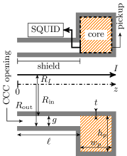
Figure 1: Coaxial-type CCC (two-dimensional meridian schematics with symmetry axis); in this variant, the CCC itself is part of the pickup loop (represented by the thick black dashed lines) and contains optionally a highly permeable magnetic core.

The keystone of the CCC’s exceptional precision is its superconducting shield which reduces the amplitude of the magnetic induction field (written as $\vec{B}$) [4], with the exception of its azimuthal component that is left intact. More precisely, by assuming a cylindrical coordinate system $(r,z,\varphi)$ and by expanding $\vec{B}$ in a Fourier series along the azimuthal direction, all Fourier modes but the zeroth one will be attenuated by the shield (when comparing the amplitude of $\vec{B}$ at the CCC opening and at the pickup loop). This property allows a measurement which is quasi independent from the position of the current carrying path through the CCC. Formally, let us assume a current $I$ flowing through a one-dimensional wire located at a radial coordinate $R_{I}$, as shown in Fig. 1. Then, the mutual inductance

$$M(R_{I})=\frac{\mathit{\Phi}(R_{I})}{I},$$ (1)

where $\mathit{\Phi}(R_{I})$ is the magnetic flux passing through the pickup loop for a given $R_{I}$, is quasi constant with respect to $R_{I}$. Evidently, $\mathit{\Phi}$ does not depend solely upon $R_{I}$, but also on the relative position of the pickup loop with respect to the wire. This aspect will be further discussed in section IV-A.

The damping of the CCC shield can be mathematically proven and quantified when considering a geometry with an axial symmetry (e.g. see [4] or [6]). However, in practice, mechanical deformations break this symmetry. Their impact may become non-negligible when considering devices with a large radius and weight. Moreover, when considering such devices, low-frequency mechanical vibrations are triggered by the acoustic environment, increasing thus the background noise sensed by the whole CCC [11, 12]. Therefore, in order to tackle the aforementioned problems, this paper aims at i) presenting a numerical framework for quantifying the impact of static mechanical deformations on the coaxial CCC shield performance; ii) determining whether static mechanical deformations impact significantly the coaxial CCC shield noise performance and iii) motivating a quasi-static approach for studying to the impact of mechanical vibrations.

This paper is organized as follows. Section II presents the numerical toolchain and the mathematical framework for simulating deformed CCCs. Afterwards, the quantity of interest used for assessing the performance of the CCC shield is discussed in section III. Subsequently, the numerical methodology used to compute this quantity is exposed in section IV and the simulation results are further presented and discussed in section V. Finally, the case of dynamic problems is treated in section VI and conclusions are drawn in section VII.

II Numerical Toolchain for Static Deformations

In order to assess the CCC performance when undergoing static deformations, a stepwise approach is employed: i) determine a deformed configuration starting from the undeformed coaxial-type CCC shown in Fig. 1 (see section II-A) and ii) compute $M(R_{I})$ for this deformed geometry (see sections II-B and II-C). Let us note that a coreless variant will be considered throughout this work, with the exception of section V-F where the case of CCCs with a magnetic core is briefly discussed. Indeed, within a coreless framework, the numerical setting can be simplified by integrating the CCC itself in the pickup loop (see section II-B for more details), as shown in Fig 1. This variant was selected in the folded-coaxial CCC shield presented in [5].

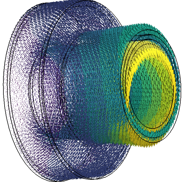
(a) Mode pattern I
(bending).

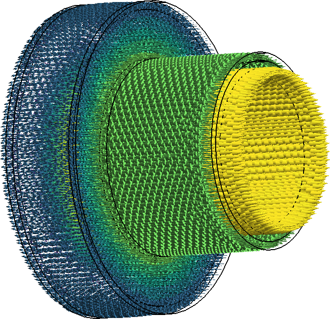
(b) Mode pattern II
(axial traction).

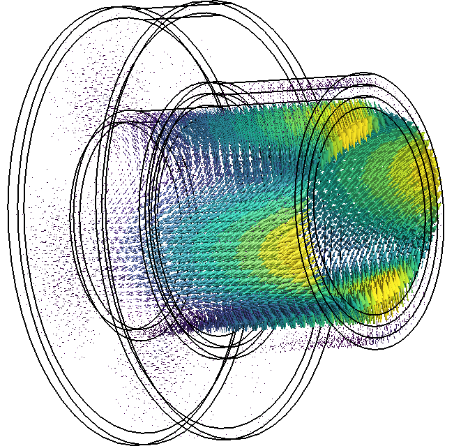
(c) Mode pattern III
(radial compression /
inner tube).

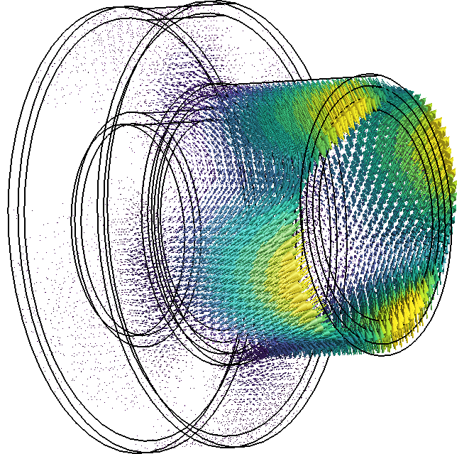
(d) Mode pattern IV
(radial compression /
outer tube).

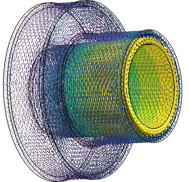
(e) Mode pattern V
(torsion).

Figure 2: Normalized mode patterns: brightest (resp. darkest) colour for $\mathinner{\!\left\lVert\vec{u}\right\rVert}=1$ (resp. $\mathinner{\!\left\lVert\vec{u}\right\rVert}=0$).

II-A Mechanical Problem and Mesh Deformation

Let us start with the mechanical problem: in order to determine a deformed geometry, we propose in this work to exploit the normal mechanical modes of the CCC. More precisely, we consider the modes of an unclamped CCC (i.e. with all six rigid body motions allowed) free of pressure/traction at its boundary. This approach is obviously computationally expensive, but i) provides meaningful deformations patterns, while considering simple boundary conditions and ii) brings a helpful insight into the dynamical performance of the CCC, as discussed further in section VI.

The mechanical modes are obtained by discretizing the time-harmonic elastodynamic equation, in terms of the displacement field $\vec{u}$, with a second-order finite element (FE) method [13]. In order to accurately discretize the axisymmetric CCC geometry, while keeping the number mesh elements as low as possible, a second-order curved mesh is used as well.

From the mode patterns determined by the mechanical solver, the most important low frequency modes are selected as shown in Fig. 2. Afterwards, a new set of meshes is generated by deforming the original axisymmetric CCC mesh according to each of the mode patterns. Regarding the amplitude of the deformation, each mode is rescaled such that $\max\mathinner{\!\left\lVert\vec{u}\right\rVert}=g/s$, where $g$ is the CCC’s air gap (see Fig. 1) and $s$ a real-valued scaling factor (see section IV-C for more details). Ultimately, this rescaled mode pattern is employed for deforming the mesh.

For reasons of completeness, let us mention that, despite the aforementioned advantages, the computation of the normal mechanical modes is inconvenient in one aspect: it cannot determine the amplitude of a deformation, as an eigenmode is defined up to a scaling factor. Such computations can become relevant when assessing that a deformed shield does not exhibit local short circuits (i.e. contact(s) between different parts of the shield that were not present in the undeformed configuration). In this regard, driven simulations (i.e. with an actual excitation field) can be carried out instead (see e.g. [13]). The impact of such short circuits is out of the scope of this work and is not further considered.

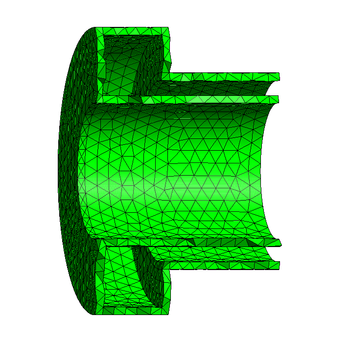
(a) Undeformed CCC
(mechanical problem).

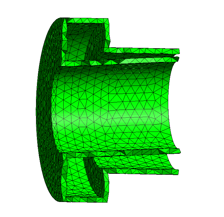
(b) Deformed CCC $\mathit{\Omega}_{\text{ccc}}$
(mechanical problem).

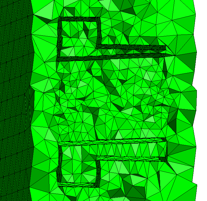
(c) Air domain $\mathit{\Omega}_{\text{air}}$
(magnetostatic problem).

Figure 3: Finite element meshes (exaggerated air gap, exaggerated deformation, meridian view).

II-B Magnetostatic Problem

The magnetic computations can now be carried out on the deformed CCC geometries. Since the problem considered here is static, the magnetostatic approximation is clearly the appropriate choice. However, one question remains: which of the vector-potential FE formulation or scalar-potential FE formulation is the most appropriate [14]? In order to answer this question, the flux coupling with the SQUID must be first discussed.

When assuming a perfect flux transformer, the SQUID will measure the magnetic induction flux passing through the pickup area. Evidently, if the CCC undergoes a deformation, this pickup area is modified. However, determining the new pickup surface $\mathcal{S}_{\mathit{\Phi}}$ is a difficult task, since the deformed geometry is known only via a discrete mesh representation and not via a computer-aided design (CAD) model. Nonetheless, when using the vector-potential formulation, this surface must not be known since

$$\mathit{\Phi}=\int_{\mathcal{S}_{\mathit{\Phi}}}\vec{B}\cdot\mathrm{d}\vec{n}=\int_{\partial\mathcal{S}_{\mathit{\Phi}}}\vec{A}\cdot\mathrm{d}\vec{t},$$ (2)

where $\vec{A}$ is the vector-potential (i.e. such that $\vec{B}=\operatorname{curl}{\vec{A}}$), $\vec{n}$ is the unit vector normal to $\mathcal{S}_{\mathit{\Phi}}$ and $\vec{t}$ is the unit vector tangent to $\partial\mathcal{S}_{\mathit{\Phi}}$ (the boundary of $\mathcal{S}_{\mathit{\Phi}}$). In other words, only the boundary of the pickup surface needs to be known when using the vector-potential. Additionally, by assuming that the CCC itself is part of the pickup loop, and since the CCC is made of an ideal superconducting material, the only portion of $\partial\mathcal{S}_{\mathit{\Phi}}$ where $\vec{A}\neq{}0$ is in the air gap (i.e. the plain line part of the pickup loop in Fig. 1). Therefore, by selecting a vector-potential formulation, the problem of determining $\mathcal{S}_{\mathit{\Phi}}$ reduces to the easier task of finding an appropriate curve $\mathit{\Gamma}_{\mathit{\Phi}}$ in the air gap defining implicitly $\mathcal{S}_{\mathit{\Phi}}$. A simple approach for determining this curve is presented in the next paragraph.

Technically, $\mathit{\Gamma}_{\mathit{\Phi}}$ is the path followed by the wires of the flux transformer between the pickup loop and the SQUID. However, to avoid the modelling of such a complex path, and since this study focuses on the CCC shield, we propose to define $\mathit{\Gamma}_{\mathit{\Phi}}$ as follows: a straight line segment defined by i) the plane of constant axial coordinate $z=\ell$ (where $\ell$ is the shield length); ii) a plane of constant azimuth $\varphi$ and iii) the endpoints located at the radial positions $r=R_{\text{in}}$ (CCC inner radius) and $r=R_{\text{out}}$ (CCC outer radius), as shown in Fig. 1 (plain black line segment). Let us mention that this definition holds for the undeformed CCC. When considering a deformed configuration, we simply assume that $\mathit{\Gamma}_{\mathit{\Phi}}$ remains a straight line segment anchored at the same endpoints (whose coordinates have been modified by the deformation).

Now that the use of a vector-potential approach has been motivated, the magnetostatic problem can be formulated. By defining the computational domain as $\mathit{\Omega}=\mathit{\Omega}_{\text{air}}\cup\mathit{\Omega}_{\text{ccc}}$, where $\mathit{\Omega}_{\text{air}}$ (resp. $\mathit{\Omega}_{\text{ccc}}$) refers to the air surrounding the CCC (resp. the CCC itself), and by designating the current carrying wire as $\mathit{\Gamma}_{I}$, the magnetostatic problem reads (in a weak sense):

$$\text{for all}~{}\vec{A}^{\prime}\in{}H_{0}(\operatorname{curl},\mathit{\Omega}_{\text{air}}),~{}\text{find}~{}\vec{A}\in{}H_{0}(\operatorname{curl},\mathit{\Omega}_{\text{air}})~{}\text{s.t.}$$

$$\int_{\mathit{\Omega}_{\text{air}}}\nu_{0}\operatorname{curl}{\vec{A}}\cdot\operatorname{curl}{\vec{A}^{\prime}}\mathrm{d}\mathit{\Omega}_{\text{air}}=\int_{\mathit{\Gamma}_{I}}I\vec{t}\cdot\vec{A}^{\prime}\mathrm{d}\mathit{\Gamma}_{I},$$ (3)

since $\vec{A}=0$ in $\mathit{\Omega}_{\text{ccc}}$ (as we assumed the CCC to be made of an ideal superconducting material) and where i) $\nu_{0}$is the magnetic reluctivity of vacuum, ii) $\vec{t}$is the unit vector tangent to $\mathit{\Gamma}_{I}$, and iii) $H_{0}(\operatorname{curl},\mathit{\Omega}_{\text{air}})$is the set of curl-conforming functions defined over $\mathit{\Omega}_{\text{air}}$ exhibiting a vanishing tangential component on $\partial\mathit{\Omega}_{\text{air}}$ [14]. This variational formulation is discretized with a second-order FE method and the unbounded domain $\mathit{\Omega}_{\text{air}}$ is truncated with a shell transformation [15]. Additionally, let us mention that the discretized system is solved with a direct method, requiring thus a gauge condition: in this work, a spanning tree gauge is exploited [16] to minimise the size of the discrete system.

II-C Mesh for the Magnetostatic Problem

As already explained in section II-A, a description of $\mathit{\Omega}_{\text{ccc}}$ (i.e. the deformed CCC geometry) is available in the form of a discrete mesh. Therefore, a hybrid description of $\mathit{\Omega}_{\text{air}}$ can be obtained, where i) its inner boundary is discretely defined by the facet elements of $\partial\mathit{\Omega}_{\text{ccc}}$ and ii) its volume and outer boundary are defined by a classical CAD model. In practice, $\mathit{\Omega}_{\text{air}}$ is a cylindrical domain truncated with a cylindrical shell.

Such hybrid descriptions are possible in the software framework offered by Gmsh [17]. However, since curved meshes are considered in this work, no guarantee exists (at the time of writing) that the final mesh obtained from such an hybrid description will be valid (i.e. with an invertible Jacobian matrix). For this reason, the mesh validity must be checked a posteriori [18]. In practice, no invalid elements where generated when using the “Frontal-Delaunay” [19] (2D mesh) and the “HXT” [20] (3D mesh) algorithms of Gmsh. To conclude this section, and for illustration purposes, both meshes (i.e. for $\mathit{\Omega}_{\text{ccc}}$ and $\mathit{\Omega}_{\text{air}}$) are depicted in Fig. 3.

II-D Software Implementation

Before concluding this section, let us mention that the above presented toolchain is implemented using a homemade FE library. Concerning the mesh related aspects, the software Gmsh is used, as previously mentioned.

III Quantity of Interest

In order to assess the CCC shield performance, the dependency of $M(R_{I})$, as defined in (1), with respect to $R_{I}$ is determined, requiring thus the computation of $\frac{\partial{}M}{\partial{}R_{I}}$. However, as different geometrical configurations will be considered, we will prefer the dimensionless quantity

$$\eta(R_{I})=\frac{\partial{}M}{\partial{}R_{I}}\frac{R_{\text{in}}}{M_{0}},$$ (4)

where $M_{0}=M(0)$. Evidently, low values of $\eta$ are associated with good position independence properties of the shield.

Additionally, let us recall that when considering undeformed coaxial-type CCCs, the shield performance is classically characterised by the dimensionless quantity [4]:

$$d=\exp\frac{\ell}{R_{\text{in}}},$$ (5)

where $\ell$ is the length of the shield. It is important to stress that the above expression relies on the assumption of an axisymmetric shield geometry. Therefore, $d$ cannot be a priori used to assess the performance of a deformed shield. Nonetheless, and by anticipating the discussion of section V, this simple criterion remains sharp, even in a deformed framework.

While this paper focuses on the shield itself, let us briefly discuss the dependence between the change of magnetic flux in the SQUID of the CCC and the current $I$ to be measured. This can be achieved by following for instance the magnetic circuit approach discussed in [5]. It is however important to stress that this requires not only the mutual inductance $M$ but also the self inductance $L$ of the pickup coil. The latter can be determined i) by setting a test current $I_{t}$ (say $1$ A) in the pickup loop, ii) by setting the current to be measured $I$ to zero, iii) by carrying out the magnetostatic computation for this setting and iv) by extracting $L$ from $\vec{A}$. It is important to stress that if more than one pickup loop is considered (see below), this procedure must be carried out for each loop (i.e. the test current is applied to only one loop at a time).

IV Numerical Methodology

By exploiting the numerical toolchain presented in section II, the quantity $M(R_{I})$ can be computed on both geometries: the undeformed and deformed ones. Afterwards, by evaluating $M$ for different values of $R_{I}$, the performance criterion $\eta$ can be approximated with a finite difference scheme. Nonetheless, before starting the simulations, a few practical questions remain to be answered: i) the angular position of the pickup surface $\mathcal{S}_{\mathit{\Phi}}$ with respect to the current carrying wire; ii) the geometric parameters of the undeformed CCC; and iii) the mode pattern used for the deformation and its amplitude. In the subsequent subsections, those three topics are addressed.

IV-A Pickup Surfaces and Current Carrying Wire

Obviously, the quantity $M(R_{I})$ is primarily impacted by the relative position of the current carrying wire with respect to the pickup surface $\mathcal{S}_{\mathit{\Phi}}$. Therefore, and in order to draw the most general picture of the CCC shield performance, different pickup surfaces $\mathcal{S}_{\mathit{\Phi}}$ must be considered. Let us recall that since $\mathcal{S}_{\mathit{\Phi}}$ is defined implicitly via $\mathit{\Gamma}_{\mathit{\Phi}}$ (see section II-B), we need hence to consider multiple paths $\mathit{\mathit{\Gamma}_{\mathit{\Phi}}}$ associated with different angular positions $\mathit{\varphi}$.

In particular, we consider in this work eight different angular positions which are uniformly distributed around the CCC, as illustrated by Fig. 4. Concerning the nomenclature, and in order to distinguish the different surfaces, the azimuthal position $\varphi$ of $\mathcal{S}_{\mathit{\Phi}}$ (or $\mathit{\Gamma}_{\mathit{\Phi}}$) will be specified as $\mathcal{S}_{\mathit{\Phi}}^{\varphi}$ (or $\mathit{\Gamma}_{\mathit{\Phi}}^{\varphi}$). This typographic convention is furthermore extended to $M(R_{I})$ and $\eta$, thus $M^{\frac{\pi}{4}}(R_{I})$ refers to the inductance associated to the pickup surface located at $\varphi=\frac{\pi}{4}$. Let us note that the first pickup surface is $\mathcal{S}_{\mathit{\Phi}}^{0}$ (or $\mathit{\Gamma}_{\mathit{\Phi}}^{0}$) by convention.

Concerning the current carrying wire $\mathit{\Gamma}_{I}$, we arbitrarily restrict its position to the meridian plane $\varphi=0$, and assume that a positive value of $R_{I}$ corresponds to a decrease of the distance between $\mathit{\Gamma}_{I}$ and $\mathcal{S}_{\mathit{\Phi}}^{0}$, as suggested in Fig. 4.

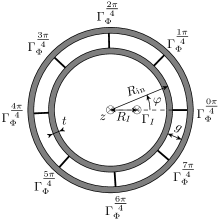
Figure 4: Location of the pickup surfaces $\mathcal{S}_{\mathit{\Phi}}^{\varphi}$ (defined implicitely via $\mathit{\Gamma}_{\mathit{\Phi}}^{\varphi}$) with respect to the current carrying wire $\mathit{\Gamma}_{I}$ (two-dimensional axial view, the entire pickup region is not shown).

IV-B Geometrical Parameters and Undeformed CCCs

In order to determine the dependence of $\eta$ with respect to geometric factors, different tuples of $R_{\text{in}}$, $\ell$ and $g$ will be studied. However, in order to avoid a too high computational cost, all possible combinations presented will not be considered. In particular, the simulations will be divided into two groups, as shown in Table I. In this table, $h_{p}$ refers to the height of the pickup surface and $w_{p}$ to the width of the pickup surface (see Fig. 1). As those two parameters define only the geometry of the pickup surface and not of the CCC shield, they are held constant and chosen as $h_{p}=w_{p}=4$ mm in this work. For all simulations, the thickness of the superconducting material is selected as $t=0.5$ mm.

TABLE I: Geometrical parameters of the coaxial CCC shield (values in mm).

Parameter set 1	$(R_{\text{in}},\ell)\in\{2.5,5,10\}\times\{8,16,32,64\}$
	with $g=0.5$, $h_{p}=4$ and $w_{p}=4$
Parameter set 2	$(g,\ell)\in\{0.25,0.5,1\}\times\{8,16,32,64\}$
	with $R_{\text{in}}=5$, $h_{p}=4$ and $w_{p}=4$

IV-C Mode Patterns and Deformed CCCs

As already mentioned, we will consider in this work the five mode patterns presented in Fig. 2. The material properties of niobium at $4.2$ K, as discussed in [21], are used. Let us note that while each CCC exhibits those mode patterns, their relative ordering (with respect to the associated resonance frequency) might differ between two geometrical configurations. The numbering given in Fig. 2 is associated with a CCC where $R_{\text{in}}=5$ mm, $\ell=8$ mm and $g=0.5$ mm. For illustration purposes, this configuration exhibits the following resonance frequencies: $f_{\text{Mode I}}\simeq 31$ Hz, $f_{\text{Mode II}}\simeq 37$ Hz, $f_{\text{Mode III}}\simeq 42$ Hz, $f_{\text{Mode VI}}\simeq 43$ Hz and $f_{\text{Mode V}}\simeq 79$ Hz. In the more realistic case of the FAIR-CCC [11], the fundamental mode has been found at approximately $80$ Hz, by assuming however that the CCC is clamped at its inner radius.

As discussed in section II-A, each mode pattern is first rescaled such that $\max\mathinner{\!\left\lVert\vec{u}\right\rVert}=g/s$ before deforming the CCC mesh accordingly. In this work, $s$ is selected in the set $s\in\{2,4,8\}$. Before concluding this section, let us indicate that because of the axial symmetry, the mode patterns are degenerated along the azimuthal direction. In order to compare similar patterns, this degeneracy is lifted by rotating the mode pattern such that $\max\mathinner{\!\left\lVert{\vec{u}}\right\rVert}$ is aligned with the angular position $\varphi=0$. Let us also note that a sign inversion might be additionally required.

V Results and Discussion

In this section, the results of the simulations described in the previous section are discussed. However, before entering into the heart of this work, let us first discuss the numerical accuracy of our computations.

V-A Numerical Accuracy

In order to determine the accuracy of the magnetostatic simulations, let us remind that in the ideal case, i.e. with the current carrying wire located directly on the symmetry axis and without deformations, the inductance $M^{\text{ideal}}$ can be computed with the formula for toroidal coils with a rectangular cross section [22]:

$$M^{\text{ideal}}=\frac{I}{\nu_{0}}\frac{w_{p}}{2\pi}\ln\frac{R_{\text{in}}+h_{p}}{R_{\text{in}}},$$ (6)

since $\vec{B}$ is fully azimuthal in this case and the CCC shield is thus transparent. While being an idealised setting, this simpler configuration offers a practical way to estimate the FE error. In the case of the parameter set $R_{\text{in}}=5$ mm and $g=0.5$ mm, the relative error is presented in Fig. 5. Let us note that this figure shows the error for different vales of $\ell\in\{8,16,32,64\}$ mm. However, in order to keep this parameter dimensionless, the coaxial damping $d(R_{\text{in}},\ell)$, as defined in equation (5), is preferred. Its systematic use will be motivated in the next subsections.

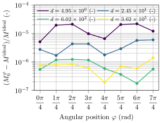
Figure 5: Accuracy of the magnetostatic FE solution for the ideal undeformed case ($R_{\text{in}}=5$ mm and $g=0.5$ mm).

From the data shown in Fig. 5, it is clear that the FE error decreases with the parameter $d$ until it reaches a plateau at approximately $10^{-6}$: it is interesting to notice that the damping properties of the CCC shield are also expressed at the discretized level. Let us also indicate that a similar behaviour of the FE error is observed for each parameter set in Table I, up to a few exceptions associated with a low damping $d<50$. We also observe that the FE error is quasi symmetric with $\varphi$ when $d=4.95$, but becomes more and more asymmetric as $d$ increases. This behaviour can be explained by the fact that the FE mesh is not perfectly symmetric. Therefore, as the numerical error decreases with increasing values of $d$, this asymmetry becomes more visible. In addition, the accuracy of the linear system solver is not infinite.

Concerning the mechanical simulations, the validity of the computations is assessed with a mesh refinement analysis based on the eigenvalues associated with the mode patterns. However, given the computational cost of such an analysis, only the smallest geometric configuration is considered with only three level of refinements. In this regard, the maximum relative change between two levels is smaller than $3~{}\%$. Nonetheless, and by anticipating the next subsections, the impact of the considered mode patterns on $\eta$ is low, and therefore highly accurate mechanical simulations are not required.

V-B Impact of $d$ on $\eta^{\varphi}$

Now that our numerical models are validated, let us enter the core of this work and discuss the influence of deformations on $\eta^{\varphi}$. To begin with, let us investigate the dependency of $\eta^{\varphi}$ with respect to the shield length, or more precisely the coaxial damping $d(R_{\text{in}},\ell)$. It is worth stressing that the CCC is deformed in this test case, while the quantity $d$ refers to the coaxial damping in the undeformed configuration.

Fig. 6 shows the behaviour of $\eta^{\varphi}$ with respect to $R_{I}/R_{\text{in}}$ for different values of $d$ and $\varphi$. In those data, i) the geometrical parameters are fixed to $R_{\text{in}}=5$ mm and $g=0.5$ mm; ii) the deformation pattern I is used; and iii) the deformation scaling factor is fixed to $s=4$. From those data, it is clear that two angular positions, namely $\varphi=\pi/2$ and $\varphi=3\pi/2$, exhibit a significantly lower value for $\eta^{\varphi}$, as compared to the other angular positions for a fixed $d$. The existence of two particular angular positions can be justified theoretically in the undeformed case, as demonstrated in appendix A. Furthermore, their precise location at $\varphi=\pi/2$ and $\varphi=3\pi/2$ is a consequence of the restriction of the current carrying wire to the plane $\varphi=0$, as also shown in appendix A. In order to improve the readability of the subsequent plots, those two special angles are omitted from now on.

Additionally, it is obvious from Fig. 6 that the higher the $d$, the lower the $\eta^{\varphi}$. In particular, for an increase of $d$ by a power of $2$, $\eta^{\varphi}$ is reduced by a power of $\sim{}2$ as well. In light of this behaviour, it is tempting to directly conclude that the intrinsic property of the CCC shield, i.e. the damping of the non-azimuthal components of $\vec{B}$ (in the sense of the Fourier decomposition discussed in the introduction), are kept despite the deformations. Nonetheless, this hypothesis must be first validated by means of other numerical experiments, as discussed in the next subsections.

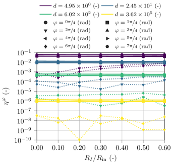
Figure 6: Impact of $d$ on $\eta^{\varphi}$ ($R_{\text{in}}=5$ mm, $g=0.5$ mm, mode pattern I and $s=4$).

V-C Impact of the Geometrical Parameters on $\eta^{\varphi}$

In order to validate our previous hypothesis, let us start with determining the impact of the inner radius $R_{\text{in}}$ on $\eta^{\varphi}$ for different values of $d(R_{\text{in}},\ell)$, which corresponds to the first data set in Table I. This influence is depicted in Fig. 7 for the case $\varphi=0$. Let us note that a similar behaviour is observed for the other angles, but only $\varphi=0$ is shown for clarity reasons. Let us also mention that the combinations $(R_{\text{in}},d)\in\{(2.5~{}\text{mm},4.95),(10~{}\text{mm},3.62\times{}10^{5})\}$ do not exist. From the data displayed in Fig. 7, it is obvious that, while $R_{\text{in}}$ affects $\eta^{\varphi}$, its impact is negligible in regard to $d$.

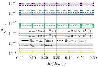
Figure 7: Impact of $R_{\text{in}}$ on $\eta^{0}$ (parameter set 1, mode pattern I and $s=4$).

In Fig. 8, the influence of the air gap size $g$ on $\eta^{\varphi}$ is shown for different values of $d(R_{\text{in}}=5~{}\text{mm},\ell)$. This case corresponds to the second data set in Table I, and only the case $\varphi=0$ is shown for the same above mentioned reasons. It is clear from Fig. 8 that an increase in $g$ leads to an increase in $\eta$. Let us note that this behaviour is expected, since larger air gap sizes are known to decrease the coaxial CCC shield performance even in the ideal undeformed case [6].

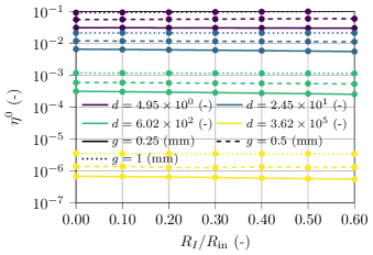
Figure 8: Impact of $g$ on $\eta^{0}$ (parameter set 2, mode pattern I and $s=4$).

V-D Impact of Deformations on $\eta^{\varphi}$

Now that the effect of the geometrical parameters are assessed for a deformed coaxial-type CCC, let us focus on the impact of the deformations themselves on $\eta^{\varphi}$. Again, the data presented below are restricted to the case $\varphi=0$ for clarity reasons, but the discussion remains valid for the other angular positions. As it can be seen in Fig. 9, the performance of the coaxial CCC shield is only mildly affected by the deformations, when compared to the impact of $d$. In particular, this figure shows $\eta^{0}$ for all five deformation patterns and for all three deformation amplitudes together with the undeformed configuration. The geometric parameters are those of the parameters set 1 in Table I restricted to $R_{\text{in}}=5$ mm. Nonetheless, the same conclusion can be drawn for the other values of $R_{\text{in}}$, which are not shown here for conciseness reasons.

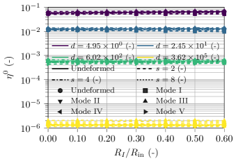
Figure 9: Impact of deformations on $\eta^{0}$ (parameter set 1 restricted to $R_{\text{in}}=5$ mm).

In order to complement the data shown in Fig. 9, let us first take the average value of $\eta^{0}$ over $R_{I}/R_{\text{in}}$, as it is clear from Fig. 9 that $\eta^{0}$ is quasi independent from $R_{I}/R_{\text{in}}$, and denote it by $\overline{\eta^{0}}$. We then compute the relative deviation $\varepsilon_{d,m,s}$ for a given value of $d$, a given deformation pattern $m$ and a given value of $s$:

$$\varepsilon_{d,m,s}=\frac{\mathinner{\!\left\lvert\overline{\eta^{0,\text{def}}_{d,m,s}}-\overline{\eta^{0,\text{und}}_{d}}\right\rvert}}{\overline{\eta^{0,\text{und}}_{d}}},$$ (7)

where $\overline{\eta^{0,\text{def}}_{d,m,s}}$ is associated with the deformed geometry and $\overline{\eta^{0,\text{und}}_{d}}$ with the undeformed one. Afterwards, we collect in Table II the maximum value of $\varepsilon_{d,m,s}$ for each $d$, that is formally

$$\varepsilon_{d}^{\max}=\max_{(m,s)}\varepsilon_{d,m,s}.$$ (8)

From these data, the relative variations $\varepsilon_{d}^{\max}$ appear to be large, but it must be noted that they are small compared with the variations induced by $d$ itself. Let us also note that the increase in $\varepsilon_{d}^{\max}$ with $d$ must be considered with care, as it might be simply due to the limit of the numerical model being reached.

$d$	$\varepsilon_{d}^{\max}$	Associated pair $(m,s)$	Associated $\overline{\eta^{0,\text{und}}_{d}}$	Associated $\overline{\eta^{0,\text{def}}_{d,m,s}}$
$4.95\times{}10^{0}$	$16$ %	$(I,2)$	$6.22\times{}10^{-2}$	$5.24\times{}10^{-2}$
$2.45\times{}10^{1}$	$16$ %	$(I,2)$	$1.26\times{}10^{-2}$	$1.06\times{}10^{-2}$
$6.02\times{}10^{2}$	$22$ %	$(IV,2)$	$5.91\times{}10^{-4}$	$4.58\times{}10^{-4}$
$3.62\times{}10^{5}$	$33$ %	$(III,2)$	$1.34\times{}10^{-6}$	$1.78\times{}10^{-6}$

TABLE II: Relative and absolute variations of the shield performance (all quantities are dimensionless, parameter set 1 restricted to $R_{\text{in}}=5$ mm).

V-E Impact of Deformations on $M^{\varphi}(0)$

So far, our discussion was focused solely on $\eta^{\varphi}$, which reflects how effective the coaxial CCC shield is in terms of position independence. While this paper aims primarily at studying this aspect, the behaviour of $M$ itself deserves nonetheless a few comments. As mentioned in the previous subsection, the value of $\eta$ is only mildly affected by deformations: it is therefore legitimate to concentrate this subsection on $M^{\varphi}(0)=M^{\varphi}_{0}$ only.

As it can be seen in Fig. 10, deformations have clearly a higher impact on $M$ than $\eta$. This behaviour is easily explained, since the value of $M$ is directly related to the pickup surface, which can undergo significant deformations. It is also unequivocal from Fig. 10 that deformations have less impact on $M_{0}$ for larger values of $d$. The reason for this is however unrelated to the magnetic properties of the coaxial CCC shield. Indeed, a deformation whose maximum amplitude is located at the tip of the CCC opening (exactly as the mode patterns in Fig. 2) is impacting less the pickup surface when $\ell$ (and thus $d$) is large, since the distance between the maximum displacement and the pickup surface is increased.

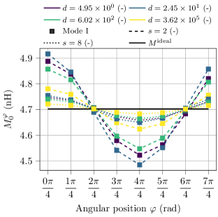
Figure 10: Impact of deformations on $M^{\varphi}(0)=M^{\varphi}_{0}$ (parameter set 1 restricted to $R_{\text{in}}=5$ mm).

V-F Summary and Additional Comment

We recognized in this section that $\eta$ can be significantly lowered when $d$ is large, even if some geometrical parameters may worsen its value mildly. Moreover, we observed that the amplitude of the deformation or the mode pattern have also a negligible impact on $\eta$ compared to $d$. For all these reasons, it is legitimate to conclude that the coaxial CCC shield keeps its intrinsic damping properties, even when considering deformations. Nonetheless, as a direct consequence of the deformations of the pickup surface, deformations have a non-negligible impact on $M$ itself.

It is also worth mentioning that we considered a coreless variant of the coaxial-type CCC, where the CCC itself is part of the pickup loop. In the case of a CCC with a highly permeable magnetic core, it is however more usual to separate shield and pickup circuit by winding a superconducting coil around the core. Nonetheless, as this variation does not modify the shield itself, our conclusions about $\eta$ and the coaxial CCC shield damping remain unchanged. Let us also note that CCCs with highly magnetic permeable materials suffer from temperature dependent drifts and low-frequency noise caused by flipping of individual magnetic domains inside the core material [5].

To conclude this section, let us recall that our model cannot allow arbitrary deformations. Indeed, large deformations with respect to the air gap my lead to new contacts within the shield (see section II-A). Those topological changes may lead to drastic modifications in the shielding properties, but are out of the scope of this paper.

VI Dynamic Problems

In the previous section, only static deformations were investigated. However, the CCC can be submitted to mechanical vibrations during operation, especially in the context of particle beam diagnostics. For this reason, the treatment of dynamic problems is also highly relevant. From an electromagnetic point of view, the position independence property of the CCC shield follows from the ability of superconducting materials to expel any interior magnetic induction field [4]. This perfect diamagnetism is attributed to shielding currents, which are in practice well described by the London theory [24], as CCCs are usually made of thick superconductors (e.g. $3$ mm in the case of the FAIR-CCC [11] or $1$ mm for the CCC discussed in [5]) held well below the critical temperature. In this theoretical framework, and by neglecting the displacement currents, the London equation do not contain any dynamics. For this reasons, the static electromagnetic properties of the CCC shield remain valid even in a dynamic context, allowing us to conclude that i) our static analysis can be applied in a dynamic context (quasi-static framework) and ii) the intrinsic performance of the coaxial CCC shield are kept, even when undergoing mechanical vibrations, at least as long as our working hypothesis are met. In particular, we assumed implicitly that the stress and strain fields do not impact the electromagnetic properties of the superconducting material. Let us note that the same holds for the magnetic core when this one is present, this latter hypothesis being however quite restrictive in practice.

VII Conclusions

Via numerical computations, we showed that the intrinsic position independence property of the coaxial CCC shield is negligibly affected by mechanical deformations. Nonetheless, as those deformations may change the size and orientation of the CCC pickup surface, the coupling inductance $M$ may be significantly affected. We furthermore discussed the case of mechanical vibrations, and showed that the above mentioned conclusions remain valid, as long as London theory remains valid, which we expect to be true in practical situations. Last but not least, let us also mention that the numerical toolchain developed in this work is not specific to the analysis of CCCs and can be used to assess the performance of any deformed superconducting magnetic shield. Additionally, this approach can be also used to analyse CCCs with other types of shielding, such as the ring or the overlapped ones.

Appendix A Why is $\eta^{\varphi}$ lower for $\varphi=\pi/2$ and $\varphi=3\pi/2$?

As already mentioned in the introduction, by expanding $\vec{B}$ in a Fourier series along the azimuthal direction, it can be shown that the coaxial CCC shield damps all Fourier modes but the zeroth one. In particular, the higher the Fourier mode, the higher the attenuation [4]. In the case of the numerical setting presented in section IV-A, the source current density $\vec{j}_{s}$ due to the current carrying wire can be formally written in a cylindrical coordinate system as (see Fig. 4):

$$\vec{j}_{s}=\frac{I}{R_{I}}\delta(\varphi)\hat{z},$$ (9)

where $\delta$ is a $2\pi$-periodic Dirac delta function and $\hat{z}$ is the unit vector oriented along the symmetry axis. It is worth mentioning that this expression is compatible with the right-hand side of (3) when restricted to $\mathit{\Gamma}_{I}$.

Let us now expand (9) in a Fourier series along $\varphi$:

$$\vec{j}_{s}=\frac{I}{R_{I}}\left(\frac{1}{2\pi}+\frac{1}{\pi}\sum_{n=1}^{\infty}\cos(n\varphi)\right)\hat{z},$$ (10)

and define its modal components as

$$\vec{j}^{0}_{s}=\frac{I}{2\pi R_{I}}\hat{z}\quad\text{and}\quad\vec{j}^{n}_{s}=\frac{I}{\pi R_{I}}\cos(n\varphi)\hat{z}~{}\forall{}n>0.$$ (11)

According to the aforementioned theory of undeformed coaxial CCC shields [4], each modal component of $\vec{j}_{s}$ will be damped, with $\vec{j}^{1}_{s}$ undergoing the lowest damping (by excluding of course $\vec{j}^{0}_{s}$ which is undamped). Therefore, when considering the angular positions $\varphi=\pi/2$ and $\varphi=3\pi/2$, it is clear that $\vec{j}^{1}_{s}=0$. Thus, the component undergoing the lowest damping is for those angles unexcited, reducing thereby $\eta^{\varphi}$ by a large factor when compared to $\varphi=0$.

References

- [1] I. K. Harvey, “A precise low temperature dc ratio transformer,” Review of Scientific Instruments, vol. 43, no. 11, pp. 1626–1629, 1972.
- [2] J. M. Williams, “Cryogenic current comparators and their application to electrical metrology,” IET Science, Measurement and Technology, vol. 5, no. 6, pp. 211–224, 2011.
- [3] J. Clarke and A. I. Braginski, eds., The SQUID Handbook I: Fundamentals and Technology of SQUIDs and SQUID Systems. Weinheim: Wiley-VCH, 2004.
- [4] K. Grohmann, H. D. Hahlbohm, D. Hechtfischer, and H. Lübbig, “Field attenuation as the underlying principle of cryo current comparators,” Cryogenics, vol. 16, no. 7, pp. 423–429, 1976.
- [5] V. Zakosarenko, M. Schmelz, T. Schönau, S. Anders, J. Kunert, V. Tympel, R. Neubert, F. Schmidl, P. Seidel, T. Stöhlker, D. Haider, M. Schwickert, T. Sieber, and R. Stolz, “Coreless SQUID-based cryogenic current comparator for non-destructive intensity diagnostics of charged particle beams,” Superconductor Science and Technology, vol. 32, no. 1, p. 014002, 2018.
- [6] N. Marsic, W. F. O. Müller, H. De Gersem, M. Schmelz, V. Zakosarenko, R. Stolz, F. Kurian, T. Sieber, and M. Schwickert, “Numerical analysis of a folded superconducting coaxial shield for cryogenic current comparators,” Nuclear Instruments and Methods in Physics Research Section A: Accelerators, Spectrometers, Detectors and Associated Equipment, vol. 922, pp. 134–142, 2019.
- [7] K. Grohmann, H. D. Hahlbohm, D. Hechtfischer, and H. Lübbig, “Field attenuation as the underlying principle of cryo-current comparators 2. Ring cavity elements,” Cryogenics, vol. 16, no. 10, pp. 601–605, 1976.
- [8] D. B. Sullivan and R. F. Dziuba, “Low temperature direct current comparators,” Review of Scientific Instruments, vol. 45, no. 4, pp. 517–519, 1974.
- [9] J. M. Williams, T. J. B. M. Janssen, G. Rietveld, and E. Houtzager, “An automated cryogenic current comparator resistance ratio bridge for routine resistance measurements,” Metrologia, vol. 47, no. 3, pp. 167–174, 2010.
- [10] M. Fernandes, R. Geithner, J. Golm, R. Neubert, M. Schwickert, T. Stöhlker, J. Tan, and C. P. Welsch, “Non-perturbative measurement of low-intensity charged particle beams,” Superconductor Science and Technology, vol. 30, no. 1, p. 015001, 2017.
- [11] P. Seidel, V. Tympel, R. Neubert, J. Golm, M. Schmelz, R. Stolz, V. Zakosarenko, T. Sieber, M. Schwickert, F. Kurian, F. Schmidl, and T. Stohlker, “Cryogenic current comparators for larger beamlines,” IEEE Transactions on Applied Superconductivity, vol. 28, no. 4, pp. 1–5, 2018.
- [12] V. Tympel, H. De Gersem, M. Fernandes, J. Golm, D. M. Haider, F. Kurian, N. Marsic, W. F. O. Müller, R. Neubert, M. Schmelz, F. Schmidl, M. Schwickert, P. Seidel, T. Sieber, T. Stöhlker, R. Stolz, J. Tan, C. Welsch, and V. Zakosarenko, “Comparative measurement and characterisation of three cryogenic current comparators based on low-temperature superconductors,” in Proceedings of the 7th International Beam Instrumentation Conference (IBIC’18), no. 7 in International Beam Instrumentation Conference, (Geneva, Switzerland), pp. 126–129, JACoW Publishing, 2018.
- [13] M. Géradin and D. J. Rixen, Mechanical Vibrations. Chichester: John Wiley & Sons, 3 ed., 2015.
- [14] A. Bossavit, Computational Electromagnetism. Cambridge, MA: Academic Press, 1998.
- [15] F. Henrotte, B. Meys, H. Hedia, P. Dular, and W. Legros, “Finite element modelling with transformation techniques,” IEEE Transactions on Magnetics, vol. 35, no. 3, pp. 1434–1437, 1999.
- [16] P. Dular, A. Nicolet, A. Genon, and W. Legros, “A discrete sequence associated with mixed finite elements and its gauge condition for vector potentials,” IEEE Transactions on Magnetics, vol. 31, no. 3, pp. 1356–1359, 1995.
- [17] C. Geuzaine and J.-F. Remacle, “Gmsh: A 3-D finite element mesh generator with built-in pre- and post-processing facilities,” International Journal for Numerical Methods in Engineering, vol. 79, no. 11, pp. 1309–1331, 2009.
- [18] A. Johnen, J.-F. Remacle, and C. Geuzaine, “Geometrical validity of curvilinear finite elements,” Journal of Computational Physics, vol. 233, pp. 359–372, 2013.
- [19] S. Rebay, “Efficient unstructured mesh generation by means of Delaunay triangulation and Bowyer-Watson algorithm,” Journal of Computational Physics, vol. 106, no. 1, pp. 125–138, 1993.
- [20] C. Marot, J. Pellerin, and J.-F. Remacle, “One machine, one minute, three billion tetrahedra,” International Journal for Numerical Methods in Engineering, vol. 117, no. 9, pp. 967–990, 2019.
- [21] M. C. Lin, C. Wang, L. H. Chang, G. H. Luo, and M. K. Yeh, “Effects of material properties on resonance frequency of a CESR-III type 500 MHz SRF cavity,” in Proceedings of the 2003 Particle Accelerator Conference, pp. 1371–1373, 2003.
- [22] E. Durand, Électrostatique et magnétostatique. Paris: Masson, 1953.
- [23] M. Arioli, J. W. Demmel, and I. S. Duff, “Solving sparse linear systems with sparse backward error,” SIAM Journal on Matrix Analysis and Applications, vol. 10, no. 2, pp. 165–190, 1989.
- [24] F. London and H. London, “The electromagnetic equations of the supraconductor,” Proceedings of the Royal Society of London A: Mathematical, Physical and Engineering Sciences, vol. 149, no. 866, pp. 71–88, 1935.