Understanding the Vulnerability of Skeleton-based
Human Activity Recognition via Black-box Attack

Abstract

Human Activity Recognition (HAR) has been employed in a wide range of applications, e.g. self-driving cars, where safety and lives are at stake. Recently, the robustness of existing skeleton-based HAR methods have been questioned due to their vulnerability to adversarial attacks [1], which causes concerns considering the scale of the implication. However, the proposed attacks require the full-knowledge of the attacked classifier, which is overly restrictive. In this paper, we show such threats indeed exist, even when the attacker only has access to the input/output of the model. To this end, we propose the very first black-box adversarial attack approach in skeleton-based HAR called BASAR. BASAR explores the interplay between the classification boundary and the natural motion manifold. To our best knowledge, this is the first time data manifold is introduced in adversarial attacks on time series. Via BASAR, we find on-manifold adversarial samples are extremely deceitful and rather common in skeletal motions, in contrast to the common belief that adversarial samples only exist off-manifold [2]. Through exhaustive evaluation, we show that BASAR can deliver successful attacks across classifiers, datasets, and attack modes. By attack, BASAR helps identify the potential causes of the model vulnerability and provides insights on possible improvements. Finally, to mitigate the newly identified threat, we propose a new adversarial training approach by leveraging the sophisticated distributions of on/off-manifold adversarial samples, called mixed manifold-based adversarial training (MMAT). MMAT can successfully help defend against adversarial attacks without compromising classification accuracy.

I Introduction

Current state-of-the-art Human Activity Recognition (HAR) solutions are mainly based on deep learning, which are vulnerable to adversarial attack [3]. This causes major concerns especially in safety and security [4], as the perturbations are imperceptible to humans but destructive to machine intelligence. Detecting and defending against attacks have been actively investigated [5]. While the research on static data (e.g. images, texts, graphs) has been widely studied, the attack on time-series data has only been recently explored  [6, 7, 8]. We investigate a specific yet important type of time series data, skeletal motions, in HAR.

Skeletal motion is widely employed in HAR to mitigate issues such as lighting, occlusion, view angles, etc [9]. Therefore, the vulnerability of skeleton-based classifiers under adversarial attack has recently drawn attention [10, 11, 1]. Albeit identifying a key issue that needs to be addressed, their methods are essentially white-box. The only attempt on black-box attack is via surrogate models, i.e. attack a classifier in a white-box manner then use the results to attack the target classifier. While white-box attack requires the full knowledge of the attacked model which is overly restrictive, black-box attack via surrogate models cannot guarantee success due to its heavy dependence on the choice of the surrogate model [1]. Is true black-box attack possible in skeleton-based HAR? To answer the question, we restrict the accessible knowledge to be only the inputs/outputs of the classifiers, and propose BASAR, the very first black-box attack method on skeleton-based activity recognition to our best knowledge.

Black-box attack on skeletal motions brings new challenges and discoveries due to their unique features compared with other data. First, a skeleton usually has less than 100 Degrees of freedom (Dofs), much smaller than previously attacked data such as images/meshes. This low dimensionality leads to low-redundancy [12], restricting possible attacks within small subspaces. Second, imperceptibility is a prerequisite for any successful attack, but its evaluation on skeletal motions is under-explored. Different from the attack where visual imperceptibility has high correlations with the perturbation magnitude (e.g. images), a skeletal motion has dynamics that are well-recognized by human perception. Any sparse attack, e.g. on individual joints or individual poses, albeit small, would break the dynamics and therefore be easily perceptible. In contrast, coordinated attacks on all joints and poses can provide better imperceptibility even when perturbations are relatively large [1]. Consequently, the perturbation magnitude alone (as in most existing methods) is not a reliable metric for skeletal motion. Last but not least, prior methods assume that adversarial samples are off the data manifold [2]. As we will show, skeletal motion is one real-world example where on-manifold adversarial samples not only exist but are rather common, raising serious concerns as these on-manifold adversarial samples are implementable.

Given a motion $\mathbf{x}$ with class label $c_{\mathbf{x}}$, BASAR aims to find $\mathbf{x}^{\prime}$ that is close to $\mathbf{x}$ (measured by some distance function) and can fool a black-box classifier such that $c_{\mathbf{x}^{\prime}}\neq c_{\mathbf{x}}$. BASAR formulates this process as a constrained optimization problem, aiming to find $\mathbf{x}^{\prime}$ that is just outside $c_{\mathbf{x}}$ with a new requirement: $\mathbf{x}^{\prime}$ being on the data manifold. The optimization is highly non-linear due to the compounded non-linearity of the classification boundary and the data manifold. The former dictates that any greedy search (e.g. gradient-based) near the boundary will suffer from local minima; while the latter means that not all perturbation directions result in equal visual quality (in-manifold perturbations tend to be better than off-manifold perturbations). Consequently, there are often conflicts between these two spaces when searching for $\mathbf{x}^{\prime}$. To reconcile the conflicts, we propose a new simple yet effective method called guided manifold walk (GMW) which can compute $\mathbf{x}^{\prime}$ that is close to $\mathbf{x}$ and also on the data manifold.

We exhaustively evaluate BASAR on state-of-the-art classifiers on multiple datasets in both untargeted and targeted attack tasks. The results show that not only is BASAR successful across models and datasets, it can also find on-manifold adversarial samples, in contrast to the common assumption that adversarial samples only exist off-manifold [2]. On par with very recent work that also found on-manifold samples in images [13], we show, for the first time, the existence and commonality of such samples in skeletal motions. We also comprehensively compare BASAR with other methods, showing the superiority of BASAR by large margins. In addition, since the perturbation magnitude alone is not enough to evaluate the attack quality, we propose a new protocol for perceptual study and conduct harsh perceptual evaluation on the naturalness, deceitfulness, and indistinguishability of the attack. The perceptual results show on-manifold adversarial examples seem more natural and realistic than regular adversarial examples. Further motivated by this observation, we recognize that on/off-manifold adversarial examples have different distributions, which forms a new more fine-grained description of the adversarial sample distribution. Consequently, we propose a new adversarial training approach called mixed manifold-based adversarial training (MMAT) to explore the interactions between on/off-manifold adversarial samples and clean samples during the adversarial training. We show that a proper mixture of adversarial samples with clean samples can simultaneously improve the accuracy and robustness, as opposed to the common assumption that there is always a trade-off between them [14, 15, 16]. Overall, the philosophy behind MMAT is general and can be potentially employed on other data/tasks, e.g. images.

Formally, we demonstrate that adversarial attack is truly a threat to human activity recognition, and systematically study their robustness towards adversaries. To this end, we

1. propose the first black-box attack method and comprehensively evaluate the vulnerability of several state-of-the-art classifiers.

2. show the existence of on-manifold adversarial samples in various datasets and provide key insights on what classifiers tend to resist on-manifold adversarial samples.

3. show on-manifold adversarial samples are truly dangerous because they are not easily identifiable under even strict perceptual studies.

4. propose a new defense approach by leveraging the sophisticated distributions of on/off-manifold adversarial samples in data augmentation, simultaneously improving robustness and accuracy.

5. propose a new perceptual study protocol to evaluate motion attack quality, addressing that there is currently no metrics suitable for evaluating motion attack quality.

This paper is an extension of our prior research [1, 17]. The improvements and extensions include: (1) a new adversarial training method for skeleton-based HAR and detailed defense evaluation, (2) additional attack experiments in new datasets, (3) new experiments integrating manifold projection with other attacks, (4) new literature review on Adversarial Defense, (5) new discussions about limitations, (6) additional details of mathematical deduction, implementation, and performance and (7) details for perceptual studies.

II Related Work

II-A Skeleton-based Activity Recognition

Early HAR research focuses on useful hand-crafted features [18, 19]. In the era of deep learning, features are automatically learnt. Motions can be treated as time series of joint coordinates and modeled by Recurrent Neural Networks [20, 21]. Motions can also be converted into pseudo-images and learned with Convolutional Neural Networks [22, 23]. Graph Convolutional Networks (GCN) recently achieve the state-of-the-art performance, by considering the skeleton as a graph (joints as the nodes and bones as edges) [24, 25, 26, 27]. Liu et al. [27] utilize disentangled multi-scale graph convolutions, which contains a unified spatial-temporal GCN operator for capturing complex spatial-temporal dependencies. Zhang et al. [26] introduce joint semantics to the GCN model, resulting in a lightweight yet effective method. Our work is complementary to HAR, by demonstrating their vulnerability to adversarial attacks and suggesting potential improvements. We extensively evaluated BASAR on state-of-the-art methods, showing that even the very recent methods with remarkable successes are still vulnerable to adversarial attacks.

II-B Adversarial Attack

II-B1 White-box Attack

Since [3], an increasing number of adversarial attack methods have been proposed in different tasks [4, 28, 29]. Most of them consider the white-box setting, where the model is accessible to the attacker. Apart from common computer vision tasks such as classification [30, 31, 32], adversarial attacks on general time series [6, 7, 8] and HAR [10, 1, 33] have attracted attention recently. Specifically on skeleton-based HAR, an adapted version of [31] is proposed in [10] to attack skeletal motions. Wang et al. [1] introduced a novel perceptual loss to achieve effective and imperceptible attack. Despite existing successes, current methods are based on the full access to the attacked models, and therefore are not very applicable in real-world scenarios since the details of classifiers are not usually exposed to the attacker. Hence, it is unclear whether the classifier vulnerability under (white-box) adversarial attack is a real threat. We on the other hand show that black-box attack is possible and is more threatening.

II-B2 Black-box Attack

The difficulties of white-box attack in the real-world motivates the black-box attack, where attackers cannot access the full information of the attacked model. A simple approach is transfer-based attack, which generates adversarial samples from one surrogate model via white-box attack [34]. Existing black-box methods on skeletal motions [10, 1] all rely on such a method, and cannot guarantee success due to the heavy dependence on the surrogate model [1]. Another approach is to use the predicted scores or soft labels (e.g. the softmax layer output) for attack [35, 36]. However, this is not truly black-box since the attacker still needs access the model. In a truly black-box setting, only the final class labels (hard-labels) can be used, such setting is also called hard-label attack. Brendel et al. [37] perform the first hard-label attack by a random walk along the decision boundary. Later optimization-based approaches are employed to search for adversarial samples, by estimating the gradient of the loss function using the information computed at the decision boundary [38, 39, 40]. Li et al. [41] explore three subspaces including spatial, frequency, and intrinsic component for attack. The Rays attack [42] employs a discrete search algorithm to reduce unnecessary searches. However, existing methods do not explicitly model the data manifold, and are hence incapable of considering the visual imperceptibility of the attack if they are adapted to attack skeletal motions.

In addition, black-box attacks on time-series has recently started to emerge [8, 6], in which one active sub-field is on a specific type of time-series task-HAR. Black-box adversaries have been developed in video-based recognition [43, 44, 45, 46], but skeleton-based HAR is still a research gap. Unlike existing black-box video-based attacks that achieve imperceptibility by constraining the pixel-wise or frame-wise perturbation magnitude measured by $l$ norms, skeletal motion is one real-world example and hence is more visually sensitive to attack. Any perturbations, albeit small, can easily break the motion dynamics, bone length, and joint angle constraints, making the adversarial samples visually identifiable. To tackle this problem, we propose the first hard-label black-box attack on skeleton-based HAR via explicitly modeling the data manifold.

II-C Adversarial Defense

After the threat of adversarial attack being identified, a spike of effort has been made to improve model robustness against attacks. Certified defense and adversarial training based methods [30, 47] are two mainstreams. The former seeks a theoretical robustness guarantee in model design; while the latter employs data augmentation in training and is more popular and successful to date.

II-C1 Certified defenses

A classifier with robustness guarantee against adversarial perturbations is said to be certifiably robust. Existing approaches achieve such robustness based on linear relaxations [48], convex relaxations [49], mixed-integer linear programs [50], Lipschitz constants [51] and so on. Lecuyer et al. [52] presented the first defense mechanism with robustness guarantee for randomized smoothing classifiers. Cohen et al. [53] employed a smoothed classifier with a tighter robustness guarantee by utilizing Neyman-Pearson lemma.

II-C2 Adversarial training

The original idea of adversarial training (AT) [3] is to train classifiers with a mixture of adversarial samples and clean data, to defend against adversarial attacks. Goodfellow et al. [30] further extended the approach by using an attacker to generate adversarial examples during AT. Madry et al.  [47] later redefined AT using robust optimization. Despite the significant progresses in AT [54], existing methods all compromise the accuracy to different extents. Early research [14, 15, 16] postulates that the trade-off between adversarial robustness and accuracy may be inherent. However, some recent works have proven that the trade-off can be mitigated or even theoretically eliminated. Semi-Supervised Learning-based methods can utilize extra data [55, 56] to mitigate the problem, and infinite data will improve the trade-off [57]. Stutz et al. [58] showed the existence of on-manifold adversarial samples, and reckon that on-manifold robustness is essentially related to the model generalization. Yang et al. [59] found if different classes are at least $2r$ apart, then there exists an ideal classifier which can defend against any attacks bounded by $r$ without compromising the accuracy.

Considering that the defense for skeleton-based HAR has been largely under-explored, we further extend [1, 17] to propose a new on-manifold adversarial training for skeleton-based HAR, with thorough evaluation and comparisons with other defense methods. The results show the proposed defense can potentially truly eliminate the trade-off between robustness and accuracy for skeletal motions.

III Methodology

We denote a motion with $n$ poses as $\mathbf{x}$ = $\{\textbf{x}^{1},\dots,\textbf{x}^{n}\}$, each pose $\textbf{x}^{t}$ = $\{q_{1},\dots,q_{m}\}$ including $m$ Dofs (joint positions or angles). A trained activity classifier $G$ maps a motion to a probabilistic distribution over classes, $G$: $\mathbf{x}\rightarrow\mathbb{R}^{C}$ where $C$ is the total number of action classes. The class label $c_{\mathbf{x}}$ then can be derived e.g. via softmax. An adversarial sample $\mathbf{x^{\prime}}$ corresponding to $\mathbf{x}$ can be found via [32]:

$$\text{minimize }\ \ L(\mathbf{x},\mathbf{x^{\prime}})\ \ \text{ s.t. }\ \ c_{\mathbf{x^{\prime}}}=c\text{ and }\mathbf{x^{\prime}}\in[0,1]^{m\times n}$$ (1)

where $L$ is the Euclidean distance. $c$ is the targeted class. Note that the constraint can also be replaced by $c_{\mathbf{x^{\prime}}}\neq c_{\mathbf{x}}$ for untargeted attack. However, simply applying this attack to skeletal motions is not sufficient because it only restricts the adversarial sample $\mathbf{x^{\prime}}$ in a hyper-cube $[0,1]^{m\times n}$. Given that human poses lie in a natural pose manifold $\mathcal{M}$ [60, 61], $\mathbf{x^{\prime}}$ can easily contain off-manifold poses which are unnatural/implausible and easily perceptible. We therefore add another constraint $\mathbf{x^{\prime}}\in\mathcal{M}$:

$$\text{minimize }\ \ L(\mathbf{x},\mathbf{x^{\prime}})\ \ \text{ s.t. }\ \ \mathbf{x^{\prime}}\in[0,1]^{m\times n},\mathbf{x^{\prime}}\in\mathcal{M}$$

$$c_{\mathbf{x^{\prime}}}=c\text{ (targeted)}\text{ or }c_{\mathbf{x^{\prime}}}\neq c_{\mathbf{x}}\text{ (untargeted)}.$$ (2)

In practice, we find that $\mathbf{x^{\prime}}\in[0,1]^{m\times n}$ is less restrictive than other constraints and always satisfied. The optimization is highly nonlinear and cannot be solved analytically. It thus requires a numerical solution.

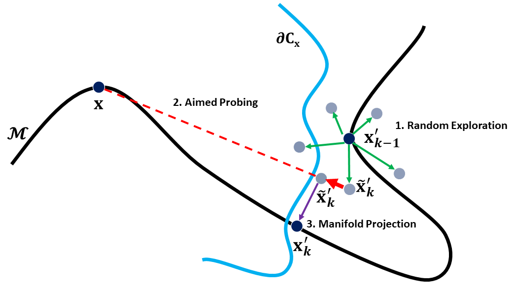
Figure 1: An abstract 2D illustration of BASAR. x is the attacked motion. $\textbf{x}^{\prime}_{k}$ is the ideal adversarial sample in iteration $k$. $\mathcal{M}$ (black line) is the natural pose manifold and $\partial C_{\mathbf{x}}$ (blue line) is the class boundary of $c_{\mathbf{x}}$. $\textbf{x}^{\prime}_{k-1}$ is the result of last iteration. $\tilde{\textbf{x}}^{\prime}_{k}$ is the intermediate result of the current iteration.

III-A Guided Manifold Walk

We propose a new method called Guided Manifold Walk (GMW) to solve Equation III. For simplicity, we start with an abstract 2D illustration of GMW on $\mathbf{x}$ shown in Figure 1. $\mathbf{x}^{\prime}_{k}$ is the ideal adversarial sample which is on-manifold and close to $\mathbf{x}$ in the $k$th iteration. Given the non-linearity of the classification boundary and the data manifold, BASAR aims to exploit the properties of both simultaneously. The GMW is an iterative approach where two major steps are alternatively conducted. One step is to find an adversarial sample that is close to $\mathbf{x}$ and the other one is to find the closest sample on the data manifold from an arbitrary off-manifold position. Since the former mainly considers the classification boundary, we design two sub-routines: random exploration and aimed probing. Similar sampling strategies have been attempted in attacking images [37]. We extend them to motions by treating a whole motion as an $n\times m$ image, with joint weighting and automatically thresholded attacks. Random exploration is to explore the vicinity of the current adversarial sample to find a random sample (step 1 in Figure 1). Aimed probing is to find a sample in proximity to $\partial C_{\mathbf{x}}$ and is closer to $\mathbf{x}$ (step 2 and 4 in Figure 1). The details are given in Section III-B and III-C. Finally, we design a sub-routine: manifold projection which is to project an off-manifold sample $\tilde{\mathbf{x}}^{\prime}_{k}$ onto $\mathcal{M}$ to obtain $\mathbf{x}^{\prime}_{k}$ (step 3 in Figure 1). This is one key element of our approach in bringing the motion manifold into adversarial attack. The algorithm overview is given in Algorithm 1, where $\lambda$ and $\beta$ are hyper-parameters and $l$ is a distance function. Next, we give details of all sub-routines.

Input: $\mathbf{x}$: attacked motion;

$\widetilde{\mathbf{x}}_{0}$: random sample, where

      $c_{\widetilde{\mathbf{x}}_{0}}=c\text{ (targeted)}\text{ or }c_{\widetilde{\mathbf{x}}_{0}}\neq c_{\mathbf{x}}\text{ (untargeted)}$;

$K$: maximum number of iterations; $\epsilon$: perturbation threshold; $\lambda$, $\beta_{1}$ and $\beta_{2}$: hyper-parameters;

Initialization: $\mathbf{x}^{\prime}_{0}=AimedProbing(\widetilde{\mathbf{x}}_{0},\mathbf{x},\beta_{1})$, so that $\mathbf{x}^{\prime}_{0}$ is adversarial and $\beta_{1}$ = update($\beta_{1}$, $\mathbf{x}^{\prime}_{0}$);

for $k=1$ to $K$ do

       $\widetilde{\mathbf{x}}_{k}=RandomExploration(\mathbf{x}^{\prime}_{k-1},\mathbf{x},\lambda)$;

       while $\widetilde{\mathbf{x}}_{k}$ is not adversarial and $\lambda\geq 10^{-10}$  do

             $\lambda$ = update($\lambda$, $\widetilde{\mathbf{x}}_{k}$);

             $\widetilde{\mathbf{x}}_{k}=RandomExploration(\mathbf{x}^{\prime}_{k-1},\mathbf{x},\lambda)$;

            

       end while

      if $\lambda\geq 10^{-10}$ then $\mathbf{x}^{\prime}_{k}=\widetilde{\mathbf{x}}_{k}$; $\lambda$ = update($\lambda$, $\widetilde{\mathbf{x}}_{k}$);

       else $\mathbf{x}^{\prime}_{k}=\mathbf{x}^{\prime}_{k-1}$; break;

        $\widetilde{\mathbf{x}}_{k}=AimedProbing(\mathbf{x}^{\prime}_{k},\mathbf{x},\beta_{1})$;

       while $\widetilde{\mathbf{x}}_{k}$ is not adversarial and $\beta_{1}\geq 10^{-10}$  do

             $\beta_{1}$ = update($\beta_{1}$, $\widetilde{\mathbf{x}}_{k}$);

             $\widetilde{\mathbf{x}}_{k}=AimedProbing(\mathbf{x}^{\prime}_{k},\mathbf{x},\beta_{1})$;

            

       end while

      if $\beta_{1}\geq 10^{-10}$ then $\mathbf{x}^{\prime}_{k}=\widetilde{\mathbf{x}}_{k}$; $\beta_{1}$ = update($\beta_{1}$, $\widetilde{\mathbf{x}}_{k}$);

       else break;

        $\widetilde{\mathbf{x}}_{k}=ManifoldProjection(\mathbf{x}^{\prime}_{k},\mathbf{x})$; $\hat{\mathbf{x}}_{k}=\widetilde{\mathbf{x}}_{k}$;

       while $\widetilde{\mathbf{x}}_{k}$ is not adversarial and $\beta_{2}\geq 10^{-10}$ do

             $\beta_{2}$ = update($\beta_{2}$, $\hat{\mathbf{x}}_{k}$);

             $\widetilde{\mathbf{x}}_{k}=AimedProbing(\mathbf{x}^{\prime}_{k},\hat{\mathbf{x}}_{k},\beta_{2})$;

            

       end while

      if $\beta_{2}\geq 10^{-10}$ then $\mathbf{x}^{\prime}_{k}=\widetilde{\mathbf{x}}_{k}$; $\beta_{2}$ = update($\beta_{2}$, $\widetilde{\mathbf{x}}_{k}$);

       else break;

        if l($\mathbf{x}^{\prime}_{k}$,$\mathbf{x}$) $<\epsilon$ then break;

      

end for

return $\mathbf{x}^{\prime}_{k}$;

Algorithm 1 Overview of the GMW

III-B Random Exploration

Random exploration is to explore in proximity to the classification boundary, by making a small step towards a random direction:

$$\widetilde{\mathbf{x}}=\mathbf{x}^{\prime}+\mathbf{W}\Delta,\text{where }\Delta=\mathbf{R}-(\mathbf{R}^{T}\mathbf{d})\mathbf{d},\ \mathbf{d}=\frac{\mathbf{x}-\mathbf{x}^{\prime}}{\|\mathbf{x}-\mathbf{x}^{\prime}\|},$$

$$\mathbf{R}=\lambda\frac{\mathbf{r}}{\|\mathbf{r}\|}\|\mathbf{x}-\mathbf{x}^{\prime}\|\text{, }r\in N(0,\mathbf{I}),$$ (3)

where $\widetilde{\mathbf{x}}$ is the new perturbed sample, $\mathbf{x}$ and $\mathbf{x}^{\prime}$ are the attacked motion and current adversarial sample. The perturbation on $\mathbf{x}^{\prime}$, $\Delta$, is weighted by $\mathbf{W}$ - a diagonal matrix with joint weights. This is based on the experiments and perceptual study which suggest that equal perturbations on different joints are not equally effective and imperceptible, e.g. perturbations on the spinal joints cause larger visual distortion but are less effective in attacks. We therefore weight them differently. $\Delta$ controls the direction and magnitude of the perturbation, and depends on two variables $\mathbf{R}$ and $\mathbf{d}$. $\mathbf{d}$ is the directional vector from $\mathbf{x}^{\prime}$ to $\mathbf{x}$. $\mathbf{R}$ is a random directional vector sampled from a Normal distribution $N(0,\mathbf{I})$ where $\mathbf{I}$ is an identity matrix, $\mathbf{I}\in R^{z\times z}$, $z=mn$, $m$ is the number of Dofs in one frame and $n$ is total frame number. This directional vector is scaled by $\|\mathbf{x}-\mathbf{x}^{\prime}\|$ and $\lambda$.

In Equation III-B, $\Delta$ is orthogonal to $\mathbf{d}$. The random exploration essentially explores in the directions that are orthogonal to the direction towards $\mathbf{x}$, within the local area around $\mathbf{x}^{\prime}$: $\mathbf{x}^{\prime}+\mathbf{W}\Delta$. This mainly aims to avoid local minima along the $\partial C_{\mathbf{x}}$ when approaching $\mathbf{x}$. Also, we introduce adaptive attack (update($\lambda$, $\widetilde{\mathbf{x}}$ in Algorithm 1). If $\widetilde{\mathbf{x}}$ is not adversarial, we decrease $\lambda$ and perform the random exploration again; otherwise, we increase $\lambda$, then enter the next sub-routine. A similar perturbation strategy to Equation III-B is employed in [37] for images, but we adapt it for skeletal motions with joint weights and adaptive attack. More details can be found in supplementary material.

III-C Aimed Probing

Aimed probing is straightforward, aiming to find a new adversarial sample between the perturbed motion and the original, so that the new sample is closer to the attacked motion and remains adversarial: $\widetilde{\mathbf{x}}=\mathbf{x}^{\prime}+\beta(\mathbf{x}-\mathbf{x}^{\prime})$, where $\beta$ is a forward step size. Similar to $\lambda$, $\beta$ is decreased to conduct the aimed probing again if $\widetilde{\mathbf{x}}$ is not adversarial; otherwise, we increase $\beta$, then enter the next sub-routine.

III-D Manifold Projection

After aimed probing and random exploration, the perturbed motion $\widetilde{\mathbf{x}}$ is often off the manifold, resulting in implausible and unnatural poses. We thus project them back to the manifold. The natural pose manifold can be regarded as poses that do not violate bone lengths or joint limits, i.e. they are realizable by humans [62]. Further, a motion is regarded as on-manifold if all its poses are on-manifold. The motion manifold can be obtained in two ways: explicit modeling [62] or implicit learning [60, 63]. Using implicit learning would require to train a data-driven model then use it for projection [60], breaking BASAR into a two-step system. Therefore we employ explicit modeling. Specifically, we replace the constraint $\mathbf{x}^{\prime}\in\mathcal{M}$ in Equation III with hard constraints on bone lengths and joint limits. We also constrain the dynamics of $\mathbf{x}^{\prime}$ to be similar to the original motion $\mathbf{x}$:

$$\min_{\mathbf{x^{\prime}}}\ \ L(\widetilde{\mathbf{x}},\mathbf{x^{\prime}})+wL(\mathbf{\ddot{x}},\mathbf{\ddot{x}^{\prime}})$$

$$\text{s.t.}\ \ B^{\prime}_{i}=B_{i}\text{ and }\theta_{j}^{\min}\leq\theta^{\prime}_{j}\leq\theta_{j}^{\max}$$

$$C_{\mathbf{x^{\prime}}}=c\text{ (targeted)}\text{ or }C_{\mathbf{x^{\prime}}}\neq C_{\mathbf{x}}\text{ (untargeted)},$$ (4)

where $\mathbf{\ddot{x}}$ and $\mathbf{\ddot{x}^{\prime}}$ are the $2nd$-order derivatives of $\mathbf{x}$ and $\mathbf{x}^{\prime}$, $w$ is a weight. Matching the $2nd$-order derivatives is proven to be important for visual imperceptibility in adversarial attack [1]. $L$ is the Euclidean distance. $B_{i}$ and $B^{\prime}_{i}$ are the $i$-th bone’s lengths of the attacked and adversarial motion respectively. When the bone lengths change from frame to frame in the original data, we impose the bone-length constraint on each frame. $\theta^{\prime}_{j}$ is the $j$-th joint angle in every pose of $\mathbf{x^{\prime}}$ and subject to joint limits bounded by $\theta_{j}^{\min}$ and $\theta_{j}^{\max}$. Essentially, the optimization above seeks an adversarial sample that is: (1) close to the perturbed motion $\tilde{\mathbf{x}}$ in terms of the Euclidean distance, (2) matching the motion dynamics to the original motion $\mathbf{x}$ and (3) on the manifold.

Equation III-D is difficult to solve, especially to satisfy both the bone length and joint limit constraints in the joint position space [11]. We therefore solve Equation III-D in two steps. First, we solve it without any constraints by Inverse Kinematics [62] in the joint angle space, which automatically preserves the bone lengths. Next, Equation III-D is solved in the joint angle space:

$$\min_{\mathbf{\theta^{\prime}}}\ \ L(\widetilde{\mathbf{\theta}},\mathbf{\theta^{\prime}})+wL(\mathbf{\ddot{\theta}},\mathbf{\ddot{\theta}^{\prime}})\ \ \text{s.t.}\ \ \theta_{j}^{\min}\leq\mathbf{\theta^{\prime}_{j}}\leq\theta_{j}^{\max},$$

$$C_{\mathbf{x^{\prime}}}=c\text{ (targeted)}\text{ or }C_{\mathbf{x^{\prime}}}\neq C_{\mathbf{x}}\text{ (untargeted)}.$$ (5)

Note that the objective function in Equation III-D is designed to match the joint angles and the joint angular acceleration. We use a primal-dual interior-point method [64] to solve Equation III-D. After solving for $\theta^{\prime}$, the joint positions of the adversarial motion are computed using Forward Kinematics. Please refer to the supplementary materials for details of mathematical deduction.

III-E Mixed On-manifold Adversarial Training

The assumption of adversarial training is that adversarial samples can help regulate classification boundaries to resist attacks [58]. A common adversarial training (AT) strategy  [47] is:

$$\min_{\theta}\mathbb{E}_{(\mathbf{x},y)\sim{D}}\ [\max_{\bm{\delta}\in{B(\epsilon)}}\mathcal{L}(\mathbf{x}+\bm{\delta},\bm{\theta},y)]$$ (6)

where $D$ is the distribution over data pairs of $\mathbf{x}\in{\mathbb{R}^{d}}$ and label $y$. $\bm{\theta}\in{\mathbb{R}^{p}}$ is the model parameters. $B(\epsilon)=\{\bm{\delta}\ |\ \|\bm{\delta}\|_{\infty}\leq\epsilon$ } is the perturbation set. $\mathcal{L}$ is a loss function, e.g. cross-entropy. During training, the perturbation $\delta$ is drawn from a prior e.g. Gaussian and uniform distribution [52], or some adversarial attack method [47], and restricted within the $\epsilon$-ball $B(\epsilon)$.

One issue in Equation 6 is that there is an underlying assumption of the structural simplicity of the adversarial sample distribution in $B(\epsilon)$, which enables the usage of well-defined priors (e.g. Gaussians). However, we argue this assumption is overly simplified. The structure of the adversarial sample distribution can be arbitrarily complex. Consequently, when drawing perturbations from a prior, a conservative prior (e.g. Gaussians with too small variances) cannot resist attacks, while an aggressive one (e.g. Gaussians with too large variances) can be detrimental to the accuracy. On the other hand, drawing perturbations via attack leads to a more guided approximation of the adversarial sample distribution, but it also ignores the different importance across different adversarial samples. As a result, existing AT methods always need to compromise between accuracy and robustness  [54].

Unlike existing methods, we explore a finer structure depicted by two distributions in $B(\epsilon)$: the distributions of on-manifold and off-manifold adversarial samples. We first assume the distribution of adversarial samples is different from the clean data [65]. Next, we further make a more fine-grained assumption: the distribution of on-manifold adversarial samples is different from that of the off-manifold adversarial samples. We expect the fine-grained distribution modeling to be able to eliminate the trade-off between accuracy and robustness, which remains unsolved currently. This is because on-manifold samples should be directly useful in simultaneously improving the accuracy and robustness, while the off-manifold samples are more aggressive and hence helpful in improving the robustness.

To this end, we propose a mixed manifold-based adversarial training (MMAT) which optimizes a hybrid loss consisting of a standard classification loss ($\mathcal{L}_{c}$), an on-manifold robustness loss ($\mathcal{L}_{on}$) and an off-manifold robustness loss ($\mathcal{L}_{off}$) term:

$$\min_{\theta}\mathbb{E}_{(\mathbf{x},y)\sim{D}}\ [\mu_{c}\mathcal{L}_{c}+\mu_{on}\mathcal{L}_{on}+\mu_{off}\mathcal{L}_{off}]$$ (7)

where $\mu_{c}$, $\mu_{on}$ and $\mu_{off}$ are weights, $\mu_{c}=1-\mu_{on}-\mu_{off}$. The losses are:

$$\mathcal{L}_{c}=\mathcal{L}(\mathbf{x},\bm{\theta},y))$$ (8)

$$\mathcal{L}_{on}=\mathcal{L}(\mathbf{x}^{\prime}_{on},\bm{\theta},y))\ \text{s.t.}\ \mathbf{x}^{\prime}_{on}\in[0,1]^{m\times n},\ \mathbf{x}^{\prime}_{on}\in\mathcal{M}$$ (9)

$$\mathcal{L}_{off}=\max\mathcal{L}(\mathbf{x}^{\prime}_{off},\bm{\theta},y)\ \text{s.t.}\ \mathbf{x}^{\prime}_{off}\in[0,1]^{m\times n}$$ (10)

Adversary Sampling: During optimization, we need to sample $\mathbf{x}^{\prime}_{on}$ and $\mathbf{x}^{\prime}_{off}$ as they cannot be described in any analytical form. We propose a black-box and a white-box sampling strategy: BASAR and SMART [1] with MMAT, named BASAR-MMAT and SMART-MMAT respectively. In BASAR-MMAT, $\mathbf{x}^{\prime}_{on}$ and $\mathbf{x}^{\prime}_{off}$ are generated with/without Manifold Projection (BASAR-NoMP). For SMART-MMAT, we propose:

$$\arg\min_{\mathbf{x}^{\prime}}\mathcal{L}=\arg\min_{\mathbf{x}^{\prime}}\ w\mathcal{L}_{c}(\mathbf{x},\mathbf{x}^{\prime})+(1-w)\mathcal{L}_{p}(\mathbf{x},\mathbf{x}^{\prime})$$ (11)

where $\mathcal{L}_{c}(\mathbf{x},\mathbf{x}^{\prime})$ is a classification loss. It can be achieved by maximizing the cross entropy between $\Phi(\mathbf{x})$ and $\Phi(\mathbf{x}^{\prime})$:$\mathcal{L}_{c}(\mathbf{x},\mathbf{x}^{\prime})=-cross\_entropy(\Phi(\mathbf{x}),\Phi(\mathbf{x}^{\prime}))$, where $\Phi$ is namely a deep neural network and $\Phi(\mathbf{x})$ is the predicted distribution over class labels. ${L}_{p}(\mathbf{x},\mathbf{x}^{\prime})$ is the perceptual loss which dictates that $\mathbf{x}^{\prime}$ should look natural. $w$ is a weight. In SMART-MMAT, we set $w=0.6$ when sampling $\mathbf{x}^{\prime}_{on}$, and $w=1$ when sampling $\mathbf{x}^{\prime}_{off}$, i.e. not considering perceptual loss.

Given the white-box setting, we can compute the gradient $\frac{\partial\mathcal{L}}{\partial\mathbf{x}^{\prime}}$, and compute $\mathbf{x}^{\prime}$ iteratively by $\mathbf{x}^{\prime}_{t+1}=\mathbf{x}^{\prime}_{t}+\epsilon f(\frac{\partial\mathcal{L}}{\partial\mathbf{x}^{\prime}_{t}},\mathbf{x}^{\prime}_{t})$ where $\mathbf{x}^{\prime}_{t}$ is $\mathbf{x}^{\prime}$ at step $t$. $f$ computes the updates and $\epsilon$ is the learning rate. We set $\mathbf{x}^{\prime}_{0}=\mathbf{x}$ and $\epsilon=0.02$. Considering that the natural motion manifold can be well described by the motion dynamics and bone lengths [60, 62, 61], we employ a perceptual loss ${L}_{p}(\mathbf{x},\mathbf{x}^{\prime})$ for remedying the dynamics and bone length error:

$$\mathcal{L}_{p}(\mathbf{x},\mathbf{x}^{\prime})=\alpha l_{dyn}+(1-\alpha)l_{bl}$$ (12)

$$l_{bl}=\frac{1}{n}\sum||BL(\mathbf{x})-BL(\tilde{\mathbf{x}})||^{2}_{2}$$ (13)

$$l_{dyn}=\sum_{n=0}^{K}\beta_{k}||\gamma(q^{k}-{q^{\prime}}^{k})||^{2}_{2}\ \ \text{where}\sum_{n=0}^{K}\beta_{k}=1$$ (14)

where $\alpha$ is a weight and set to 0.3 for our experiments. $l_{bl}$ penalizes any bone length deviations in every frame where $n$ is the total frame number. $BL$ computes the bone lengths in each frame. $l_{dyn}$ is the dynamics loss. We use a strategy called derivative matching. It is a weighted (by $\beta_{k}$) sum of $l_{2}$ distance between $q^{k}$ and ${q^{\prime}}^{k}$, where $q^{k}$ and ${q^{\prime}}^{k}$ are the $k$th-order derivatives of the clean sample and its adversary respectively. $\gamma$ is a weight matrix. This is because a dynamical system can be represented by a collection of partial derivatives, each of which encodes information at a different order. For human motions, we empirically consider the first three orders: position, velocity and acceleration, e.g. $K=2$. High-order information can also be considered but would incur extra computation.

IV Attack Experiments

IV-A Target Models and Datasets

We select three models: STGCN [24], MS-G3D [27] and SGN [26], and four benchmark datasets: HDM05 [66], NTU60 [67], Kinetics [68] and UAV-Human [69] for experiments. HDM05 has 130 action classes, 2337 sequences from 5 subjects. Its high quality makes it suitable for our perceptual study where any visual difference between the adversarial and the original motion easily noticeable. We process HDM05 following [1] and train the target models achieving 87.2%, 94.4%, 94.1% on STGCN, MS-G3D and SGN respectively. NTU60 [67] includes 56578 skeleton sequences with 60 action classes from 40 subjects. Due to the large intra-class and viewpoint variations, it is ideal for verifying the effectiveness and generalizability of our approach. Kinetics 400 [68] is a large and highly noisy dataset taken from different YouTube Videos. The skeletons are extracted by Openpose [70], consisting of over 260000 skeleton sequences. Since SGN is not trained on it, we follow [26] to preprocess Kinetics skeletons and then train the model. UAV-Human [69] is a challenging benchmark since it was collected by an unmanned aerial vehicle, containing 22476 skeleton sequences. The queries can be slow for large target models, so we randomly sample motions to attack. We gradually increase the number of motions to attack until all evaluation metrics (explained below) stabilize, so that we know the attacked motions are sufficiently representative in the dataset. The implementation details are in the supplementary material.

IV-B Evaluation Metrics

We employ the success rate as for evaluation. In addition, to further numerically evaluate the quality of the adversarial samples, we also define metrics between the original motion $\mathbf{x}$ and its adversarial sample $\mathbf{x}^{\prime}$, including the averaged joint position deviation $l=\frac{1}{nN}\sum_{j=0}^{N}\|\mathbf{x}^{(j)}-\mathbf{x}^{{}^{\prime}(j)}\|_{2}$, the averaged joint acceleration deviation $\Delta a=\frac{1}{nON}\sum_{j=0}^{N}\|\mathbf{\ddot{x}}^{(j)}-\mathbf{\ddot{x}}^{{}^{\prime}(j)}\|_{2}$, the averaged joint angular acceleration deviation $\Delta\alpha=\frac{1}{nON}\sum_{j=0}^{N}\|\mathbf{\ddot{\theta}}^{(j)}-\mathbf{\ddot{\theta}}^{{}^{\prime}(j)}\|_{2}$, and the averaged bone-length deviation percentage $\Delta B/B=\frac{\sum_{j=0}^{N}\sum_{i=0}^{T}((B_{i}^{(j)}-B_{i}^{{}^{\prime}(j)})/B_{i}^{(j)})}{TN}$, where $N$ is the number of adversarial samples. $O$ and $T$ are the total number of joints and bones in a skeleton. $n$ is the number of poses in a motion. We also investigate the percentage of on-manifold (OM) adversarial motions. An attack sample is regarded as on-manifold if all its poses respect the bone-length and joint limit constraints. Finally, since Kinetics and UAV-Human has missing joints, it is impossible to attack it in the joint angle space. So we only attack it in the joint position space. Consequently, $\Delta\alpha$ and OM cannot be computed on Kinetics and UAV-Human.

IV-C Quantitative Evaluation

TABLE I: Untargeted attack on HDM05 (top), NTU (middle) and Kinetics (bottom). All attacks have a 100% success rate. $l$: averaged joint position deviation; $\Delta$a: averaged joint acceleration deviation; $\Delta\alpha$: averaged joint angular acceleration deviation; $\Delta$B/B: averaged bone-length deviation percentage; on-manifold sample percentage (OM). MP means Manifold Projection.

Models		$l$$\downarrow$	$\Delta a$$\downarrow$	$\Delta\alpha\downarrow$	$\Delta B/B$$\downarrow$	OM$\uparrow$
STGCN	MP	0.13	0.05	0.11	0.00%	99.55%
	No MP	0.10	0.04	0.34	0.66%	0.00%
MSG3D	MP	0.76	0.12	0.49	1.78%	0.13%
	No MP	0.70	0.09	0.82	1.81%	0.00%
SGN	MP	11.53	1.92	6.70	9.60%	60.52%
	No MP	7.93	2.00	14.36	39.64%	0.00%
STGCN	MP	0.08	0.02	0.07	4.82%	4.68%
	No MP	0.10	0.02	0.09	5.57%	1.82%
MSG3D	MP	0.08	0.03	0.12	8.14%	0.86%
	No MP	0.12	0.03	0.17	10.02%	0.57%
SGN	MP	0.28	0.08	0.21	11.11%	28.95%
	No MP	0.30	0.10	0.42	28.00%	4.55%
STGCN	MP	0.05	0.0057	n/a	2.54%	n/a
	No MP	0.07	0.0062	n/a	3.53%	n/a
MSG3D	MP	0.10	0.011	n/a	5.16%	n/a
	No MP	0.10	0.012	n/a	5.69%	n/a
SGN	MP	0.12	0.020	n/a	4.23%	n/a
	No MP	0.13	0.022	n/a	6.93%	n/a

To initialize for untargeted attack, we randomly sample a motion $\mathbf{x}^{\prime}$ for a target motion $\mathbf{x}$ where $c_{\mathbf{x}^{\prime}}\neq c_{\mathbf{x}}$. For HDM05, we randomly select 700 motions to attack STGCN, MSG3D and SGN. For NTU, Kinetics and UAV-Human, we randomly sample 1200, 500 and 500 motions respectively. The maximum iterations are 500, 1000, 1000 and 2000 on HDM05, Kinetics, UAV-Human and NTU respectively. The results are shown in Table I. Note BASAR achieves 100% success in all tasks. Here we also conduct ablation studies (MP/No MP) to show the effects of the manifold projection. First, the universal successes across all datasets and models demonstrate the effectiveness of BASAR. The manifold projection directly affects the OM results. BASAR can generate as high as 99.55% on-manifold adversarial samples. As shown in the perceptual study later, the on-manifold samples are very hard to be distinguished from the original motions even under very harsh visual comparisons.

TABLE II: Targeted attack on HDM05 (top), NTU (middle) and Kinetics (bottom). All attacks have a 100% success rate.

Models		$l$$\downarrow$	$\Delta a$$\downarrow$	$\Delta\alpha\downarrow$	$\Delta B/B$$\downarrow$	OM$\uparrow$
STGCN	MP	4.97	0.10	0.65	3.44%	56.98%
	No MP	6.25	0.09	0.92	5.85%	0.00%
MSG3D	MP	4.34	0.12	0.71	4.51%	1.64%
	No MP	4.35	0.11	1.01	5.08%	0.00%
SGN	MP	16.31	1.28	6.97	12.29%	20.96%
	No MP	16.13	1.63	13.28	29.86%	0.00%
STGCN	MP	0.37	0.03	0.25	9.73%	0.63%
	No MP	0.38	0.04	0.16	11.55%	0.16%
MSG3D	MP	0.36	0.05	0.24	15.43%	0.00%
	No OP	0.40	0.06	0.27	17.72%	0.00%
SGN	MP	1.28	0.09	0.38	28.24%	2.63%
	No MP	1.35	0.10	0.53	39.43%	0.00%
STGCN	MP	0.63	0.03	n/a	29.10%	n/a
	No MP	0.67	0.03	n/a	31.48%	n/a
MSG3D	MP	0.56	0.05	n/a	27.26%	n/a
	No MP	0.57	0.07	n/a	28.35%	n/a
SGN	MP	1.51	0.18	n/a	68.45%	n/a
	No MP	1.54	0.19	n/a	72.09%	n/a

For targeted attack, we randomly select the same number of motions from each dataset as in untargeted attack, with maximum 3000 iterations. To initiate a targeted attack on $\mathbf{x}$, we randomly select a $\mathbf{x}^{\prime}$ where $C_{\mathbf{x}^{\prime}}$ = $c$ and $c$ is the targeted class. The results are shown in Table II. All attacks achieve 100% success. The targeted attack is more challenging than the untargeted attack [1], because the randomly selected label often has completely different semantic meanings from the original one. Attacking an ‘eating’ motion to ‘drinking’ is much easier than to ‘running’. This is why the targeted attack in general has worse results than untargeted attack under every metric. Even under such harsh settings, BASAR can still produce as high as 56.98% on-manifold adversarial samples. The performance variation across models is consistent with the untargeted attack.

We also test BASAR on UAV-Human (Table III). The data quality of UAV-Human is similar to Kinetics and so is the attack performance. Overall, BASAR with manifold projection can improve the attack quality via reducing the $l$, $\Delta a$ and $\Delta B/B$.

TABLE III: STGCN Attack on UAV-Human. SR means attack success rate.

Attack Type		$l$$\downarrow$	$\Delta a$$\downarrow$	$\Delta B/B$$\downarrow$	SR
Untargeted	No MP	21.83	11.41	8.05%	100%
	MP	17.68	9.30	6.81%	100%
Targeted	No MP	69.51	32.24	28.77%	63.91%
	MP	60.07	30.59	25.10%	63.07%

Performance. The query time and number of queries for all experiments are shown in the supplementary material. Our naive implementation is sequential and did not make use of parallel computing. A GPU implementation will be significantly faster.

IV-D Classifier Robustness

From the varying performances across target models and attack modes, we can see that classifiers are not equally gullible. SGN, in general, is the hardest to fool, requiring larger perturbation compared with STGCN and MSG3D (Table I-II). This includes both joint-angle and joint-position attack. We speculate that it has to do with the features that SGN uses. Unlike STGCN and MSG3D which use raw joints and bones and rely on networks to learn good features, SGN also employs semantic features, where different joint types are encoded in learning their patterns and correlations. This requires large perturbations to bring the motion out of its pattern. Therefore, semantic information improves its robustness against attacks, as larger perturbations are more likely to be perceptible. Although SGN sometimes has a higher OM percentage, we find that some OM motions have noticeable differences from the original motions. In other words, unlike STGCN and MSG3D where a higher OM percentage indicates more visually indistinguishable adversarial samples, some OM samples of SGN look natural, can fool the classifier and probably can fool humans when being observed independently, but are unlikely to survive strict side-by-side comparisons with the original motions. Next, MSG3D is slightly harder to fool than STGCN. Although both use joint positions, MSG3D explicitly uses the bone information, which essentially recognizes the relative movements of joints. The relative movement pattern of joints helps resist attack.

To further verify our analysis, we employ an ablation study to investigate the relation between the number of queries and metrics, shown in Fig 2. Being consistent with our analysis, compared with STGCN and MSG3D, SGN usually converges faster but it is difficult for BASAR to further improve the adversarial sample as it does on STGCN and MSG3D. We speculate that this is due to the semantic information that SGN uses prevents small perturbations from altering the class labels. More details can be found in the supplementary materials.

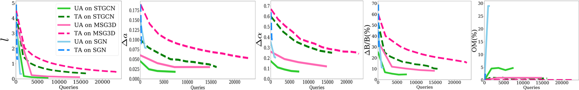
Figure 2: Metrics versus number of queries on NTU with STGCN, MSG3D and SGN.

IV-E Qualitative Evaluation

Random attacks often converge to a few classes in untargeted attack, e.g., actions on STGCN tends to be attacked into ‘clapping’(9) and ‘Use a fan’(48) on NTU, as shown in Figure 3. We call them high-connectivity classes. Since untargeted attack starts from random motions, it is more likely to find adversaries that are close to the original motion. Usually these adversaries are in classes that share boundaries with the original class. These high-connectivity classes share boundaries with many classes so that random attacks are more likely to land in them. In addition, the connectivity of classes heavily depends on the classifier itself hence different classifiers have different high-connectivity classes. Fuller results and analysis are in the supplementary materials.

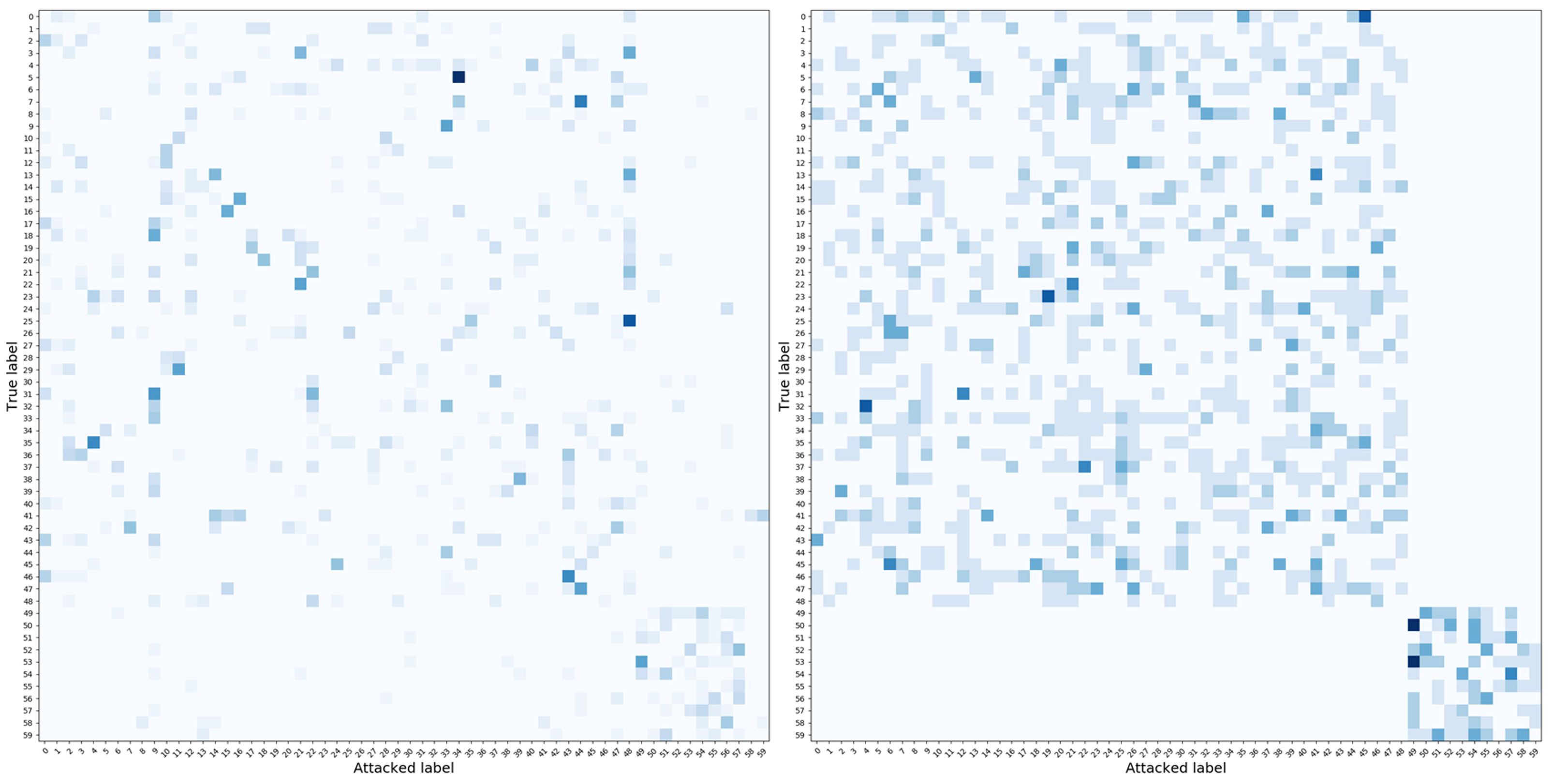
Figure 3: Confusion matrix of STGCN on NTU. Left: untargeted attack, Right: targeted attack. The darker the cell, the higher the value.

IV-F Perceptual Study

One key difference between our work and existing work is that we employ both numerical accuracy and rigorous perceptual studies to evaluate the success of attacks. Imperceptibility is a requirement for any adversarial attack. All the success shown above would have been meaningless if the attack were noticeable to humans. To evaluate imperceptibility, rigorous perceptual studies are needed for complex data, as the numerical success can always be achieved by sacrificing the imperceptibility [1]. Therefore, we propose a new perceptual study protocol which includes three studies: Deceitfulness, Naturalness and Indistinguishability. Since we have 36 scenarios (models vs datasets vs attack types vs MP/No MP), it is unrealistic to exhaustively cover all conditions. We choose HDM05 and untargeted attack for our perceptual studies. We exclude NTU and Kinetics as they contain severe and noticeable noises. Our preliminary study shows that it is hard for people to tell if a motion is attacked therein. The quality of HDM05 is high where perturbations can be easily identified. In total, we recruited 50 subjects and details of the subjects can be found in the supplementary material.

Deceitfulness. We first test whether BASAR visually changes the meaning of the motion and whether the meaning of the original motion is clear to the subjects. In each user study, we randomly choose 45 motions (15 from STGCN, MSG3D and SGN respectively) with the ground truth label and after-attack label for 45 trials. In each trial, the video is played for 6 seconds then the user is asked the question,‘which label best describes the motion? and choose Left or Right’, with no time limits.

Naturalness. This ablation study aims to test whether on-manifold adversarial samples look more natural than off-manifold samples. We design two settings: MP and No MP. MP refers to BASAR, with Manifold Projection. No MP is where the proposed method without Manifold Projection. In each study, 60 (20 from STGCN, MSG3D and SGN respectively) pairs of motions are randomly selected for 60 trials. Each trial includes one from MP and one from No MP. The two motions are played together for 6 seconds twice, then the user is asked, ‘which motion looks more natural? and choose Left, Right or Can’t tell’, with no time limits.

Indistinguishability. Indistinguishability is the strictest test to see whether adversarial samples by BASAR can survive a side-by-side scrutiny. In each user study, 40 pairs of motion are randomly selected, half from STGCN and half from MSG3D. For each trial, two motions are displayed side by side. The left motion is always the original and the user is told so. The right one can be original (sensitivity) or attacked (perceivability). The two motions are played together for 6 seconds twice, then the user is asked, ‘Do they look same? and choose Yes or No’, with no time limits. This user study serves two purposes. Perceivability is a direct test on indistinguishability while sensitivity aims to screen out users who tend to choose randomly. We discard any user data which falls below 80% accuracy on the sensitivity test.

IV-F1 Results

The average success rate of Deceitfulness is 79.64% across three models, with 88.13% , 83.33%, 67.47% on STGCN, MS-G3D and SGN respectively. This is consistent with our prediction because SGN requires larger perturbations, thus is more likely to lead to the change of the motion semantics. Next, 85% of the on-manifold adersarial samples looks more natural than off-manifold samples. This is understandable as manifold projection not only makes sure the poses are on the manifold, but also enforces the similarity of the dynamics between the attacked and original motion. Finally, the results of Indistinguishability are 89.90% on average. BASAR even outperforms the white-box attack (80.83%) in [1]. We further look into on-manifold vs off-manifold. Both samples are tested in Indistinguishability, but 94.63% of the on-manifold samples fooled the users; while 84.69% of the off-manifold samples fooled the users, showing that on-manifold samples are more deceitful. The off-manifold samples which successfully fool the users contain only small deviations.

IV-G Comparison

Since BASAR is the very first black-box adversarial attack method on skeletal motions, there is no baseline for comparison. So we employ methods that are closet to our approach as baselines. The first is SMART [1] which is a white-box approach. Although it can deliver a black-box attack, it needs a surrogate model. According to their work, we choose HRNN [20] and 2SAGCN [25] as the surrogate models. The second baseline is MTS [8] which is a black-box method but only on general time-series. It is the most similar method to BASAR but does not model the data manifold. Another baseline is BA [37], a decision-boundary based attack designed for images. We choose HDM05 and NTU for comparisons. For each comparison, we randomly select 1200 and 490 motions from NTU and HDM05. Since MTS is not designed for untargeted attack, we only compare BASAR with it on the targeted attack.

Table IV lists the success rates of all methods. BASAR performs the best and often by big margins. In the targeted attack, the highest among the baseline methods is merely 30.31% which is achieved by SMART on HDM05/MSG3D. BASAR achieves 100%. In the untargeted attack, the baseline methods achieve higher performances but still worse than BASAR. SMART achieves as high as 99.33% on NTU/MSG3D. However, its performance is not reliable as it highly depends on the chosen surrogate model, which is consistent with [1]. In addition, we further look into the results and find that SMART’s results are inconsistent. When the attack is transferred, the result labels are often different from the labels obtained during the attack.

We find that BA can also achieve 100% success. However, BA is designed to attack image data and does not consider the data manifold. We therefore compare detailed metrics and show the results in Table V. BA is in general worse than BASAR under every metric. The worst is the bone-length constraint violation. Visually, the skeletal structure cannot be observed at all. This happens for both the untargeted and the targeted attack across all datasets and models. This is understandable because BA does not consider the data manifold, while BASAR assumes that in-manifold perturbations provide better visual quality. One qualitative comparison with BA can be found in Figure 4.

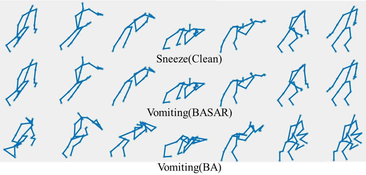
Figure 4: The visual comparison with BA. The first row is the clean motion labeled as ‘Squeeze’. The second row is the adversarial motion generated by BASAR and misclassified as ‘Vomiting’. The third row is the adversarial motion generated by BA and misclassified as ‘Vomiting’.

TABLE IV: Attack success rate comparison with baseline methods.

Models	Attacked Method	Untargeted Attack		Targeted Attack
		HDM05	NTU	HDM05	NTU
STGCN	BASAR	100%	100%	100%	100%
	MTS	n/a	n/a	3.27%	12.00%
	SMART(HRNN)	66.87%	89.25%	3.20%	2.27%
	SMART(2SAGCN)	86.10%	12.88%	2.33%	0.19%
MSG3D	BASAR	100%	100%	100%	100%
	MTS	n/a	n/a	2.18%	12.90%
	SMART(HRNN)	86.88%	99.33%	30.31%	1.16%
	SMART(2SAGCN)	88.73%	3.08%	2.46%	0.00%
SGN	BASAR	100%	100%	100%	100%
	MTS	n/a	n/a	2.91%	0.00%
	SMART(HRNN)	89.25%	98.25%	29.69%	1.42%
	SMART(2SAGCN)	0.41%	97.75%	3.28%	1.83%

TABLE V: Boundary Attack (BA) on HDM05 (top), NTU (bottom). UA/TA refers Untargeted/Targeted Attack.

Models		l$\downarrow$	$\Delta$a$\downarrow$	$\Delta\alpha\downarrow$	$\Delta$B/B$\downarrow$	OM$\uparrow$
STGCN	UA	1.44	0.65	4.74	10.60%	0.00%
	TA	8.83	0.17	1.60	8.56%	0.00%
MSG3D	UA	1.17	0.36	2.81	6.00%	0.00%
	TA	7.93	0.10	1.07	7.49%	0.00%
SGN	UA	13.35	3.45	21.96	75.11%	0.00%
	TA	15.40	1.52	11.77	29.45%	0.00%
STGCN	UA	1.04	0.47	1.97	235.10%	0.00%
	TA	0.41	0.08	0.37	35.00%	0.00%
MSG3D	UA	1.24	1.73	2.38	911.7%	0.00%
	TA	0.27	0.07	0.34	25.72%	0.00%
SGN	UA	0.22	0.28	1.26	125.57%	3.60%
	TA	0.42	0.15	0.66	65.31%	0.17%

IV-G1 Effectiveness of Manifold Projection

The manifold projection is a general operation which can theoretically work with other attackers. To verify this, we adapt Rays [42], a state-of-the-art decision-based attack for images, to attack motions by treating a motion sample as an image. Based on our experiments, Rays fails in targeted attack even with manifold projection, which is not surprising as it is not designed for attacking motions. Therefore, we only report the untargeted attack results. The model queries are the same as BASAR. As shown in Table VI, Rays-MP with manifold projection can always improve the attack success rate and the attack quality via reducing the l, $\Delta$a, $\Delta\alpha$ and $\Delta$B/B metrics. Moreover, Rays-MP can generate more natural adversarial motions.

TABLE VI: The results of Rays and Rays with manifold projection(Rays-MP) on HDM05(top) and NTU 60(bottom). $l_{\infty}$ means the $l_{\infty}$ norm distance between adversarial examples and original examples. SR means attack success rate. We show the best performance with bold.

Models	Attacks	Numerical Evaluation					$l_{\infty}$
		l$\downarrow$	$\Delta$a$\downarrow$	$\Delta\alpha\downarrow$	$\Delta$B/B$\downarrow$	OM$\uparrow$	$l_{\infty}$	SR$\uparrow$
STGCN	Rays	0.08	0.015	0.19	0.02%	27.2%	0.5	100%
	Rays-MP	0.07	0.013	0.13	0.01%	56.7%		100%
MSG3D	Rays	1.67	0.07	0.28	0.11%	0%	0.5	95.2%
	Rays-MP	1.57	0.06	0.25	0.07%	3.1%		96.9%
SGN	Rays	1.35	0.17	0.2	0.1%	60.8%	0.5	73.1%
	Rays-MP	0.89	0.06	0.1	0.0%	94.0%		96.0%
STGCN	Rays	0.061	0.028	0.019	4.6%	2.2%	0.05	99.9%
	Rays-MP	0.056	0.026	0.018	4.2%	4.8%		100%
MSG3D	Rays	0.069	0.0154	0.050	2.86%	1.2%	0.05	98.8%
	Rays-MP	0.039	0.0146	0.047	2.61%	3.8%		100%
SGN	Rays	0.19	0.003	0.0006	0.32%	95.9%	0.05	95.9%
	Rays-MP	0.07	0.0003	0.0001	0.27%	99.3%		98.5%

V Defense Experiments

V-A Experiment Setup

(A) Datasets and Models: We evaluate MMAT on HDM05 [66] using STGCN [24], MSG3D [27] and SGN [26]. NTU 60 [67] and Kinetics [68] are excluded for their extensive noises making it difficult to evaluate the effects of on-manifold samples in AT. We set the initial learning rate to 0.05 and batch size 64 on STGCN, the initial learning rate 0.025 and batch size 32 on MSG3D. For other settings we follow [24, 27, 26] to train these networks. (B) Adversarial sample sampling: For BASAR-MMAT, We utilize BASAR to attack with 500 iterations and BASAR-NoMP with 1 iteration for training. Empirically, BASAR with 500 iterations can guarantee that most of the adversarial examples are on the manifold, and BASAR-NoMP with 1 iteration can generate powerful adversaries while not severely compromising accuracy. For SMART-MMAT, we use SMART-50 (SMART with 50 iterations) for training. (C) Defense Evaluation: After adversarial training, we attack the trained model with BASAR-NoMP with 500 iterations, as it generates more violent attacks than BASAR. We also employ SMART-200 [1] and CIASA-200 [10] to test the classifier robustness under white-box attacks. (D) Weights: Since there are three weights in our adversarial training loss, we conduct an ablation study in different settings to evaluate their impacts, including (1) standard training ($\mu_{c}=1$), (2) mixture training with on-manifold adversarial samples and clean samples ($\mu_{off}=0$), (3) mixture training with on-manifold, off-manifold adversarial samples and clean samples. More settings can be found in the supplementary material.

V-B Evaluation Results

We first show the defense results of BASAR-MMAT with the best overall performance under every loss setting across different models (more results are in supplementary materials) in Table VII. We observe BASAR-MMAT can simultaneously improve the accuracy and robustness of all three models. The accuracy even outperforms the prior arts in standard training ($+4\%$, $+1.5\%$, $+0.6\%$ on STGCN, MSG3D, SGN respectively). This is also different from existing AT methods [54], which have to determine the trade-off between accuracy and robustness, BASAR-MMAT can achieve both goals. We speculate that this is because on-manifold adversarial samples can be essentially treated as unobserved ground truth data, which is strongly related to the generalization error [13]. Therefore, incorporating such samples into training naturally boosts the accuracy. Meanwhile, they help move boundaries to include the surrounding areas of the data, and hence improve the robustness.

The optimal weighting however varies across models. For STGCN and MSG3D, the effects of on/off-manifold adversarial samples are consistent with our expectation, i.e. on-manifold adversarial examples mainly contributing to improving accuracy while off-manifold adversarial examples mainly contributing on improving robustness. Somewhat surprisingly, the results on SGN show that on-manifold samples alone can achieve both goals, and adding off-manifold samples could worsen the performance (the last and penultimate row in Table VII). We speculate that this is largely due to the structure and geometry of the decision boundaries of different models. Nevertheless, BASAR-MMAT can always achieve better accuracy and robustness. Next, we show the SMART-MMAT results in Table VIII. Similarly, SMART-MMAT has consistent robustness performance across various tested attacks, and does not compromise standard accuracy. We leave the performance variation analysis across BASAR-MMAT and SMART-MMAT to Section V-C.

TABLE VII: Robustness of BASAR-MMAT against BASAR-NoMP. Top: STGCN, Middle: MSG3D, Bottom: SGN. Acc is the classification accuracy, i.e. average accuracy on clean data.

$\mu$	$l\uparrow$	$\Delta a\uparrow$	$\Delta B/B\uparrow$	Acc$\uparrow$
$\mu_{c}=1$, $\mu_{on}=0$,  $\mu_{off}=0$	0.10	0.04	0.66%	87.2%
$\mu_{c}=0.4$, $\mu_{on}=0.6$,  $\mu_{off}=0$	0.76	0.17	2.85%	90.0%
$\mu_{c}=0.4$, $\mu_{on}=0.2$,  $\mu_{off}=0.4$	2.07	0.67	10.91%	91.2%
$\mu_{c}=1$, $\mu_{on}=0$,  $\mu_{off}=0$	0.70	0.09	1.81%	94.4%
$\mu_{c}=0.4$, $\mu_{on}=0$,  $\mu_{off}=0.6$	4.53	0.86	15.86%	94.4%
$\mu_{c}=0.6$, $\mu_{on}=0.2$,  $\mu_{off}=0.2$	4.09	0.79	14.15%	95.9%
$\mu_{c}=1$, $\mu_{on}=0$,  $\mu_{off}=0$	7.93	2.00	39.64%	94.1%
$\mu_{c}=0.6$, $\mu_{on}=0$,  $\mu_{off}=0.4$	10.97	1.60	29.39%	94.1%
$\mu_{c}=0.6$, $\mu_{on}=0.4$,  $\mu_{off}=0$	14.85	3.76	80.26%	94.7%

TABLE VIII: Robustness of SMART-MMAT against white-box attacks with different iterations. Top: STGCN, Middle: MSG3D, Bottom: SGN. ’SMART’ and ’CIASA’ are the attack success rate of SMART and CIASA. Acc is the classification accuracy, i.e. average accuracy on clean data.

$\mu$	SMART		CIASA		Acc
	@50	@200	@50	@200
$\mu_{c}=1$, $\mu_{on}=0$,  $\mu_{off}=0$	95.75%	99.33%	97.99%	99.33%	87.2%
$\mu_{c}=0.4$, $\mu_{on}=0.6$,  $\mu_{off}=0$	5.80%	29.01%	6.69%	32.59%	90.6%
$\mu_{c}=0.2$, $\mu_{on}=0.6$,  $\mu_{off}=0.2$	5.80%	31.47%	5.80%	33.40%	91.0%
$\mu_{c}=1$, $\mu_{on}=0$,  $\mu_{off}=0$	92.96%	98.44%	93.54%	95.56%	94.4%
$\mu_{c}=0.6$, $\mu_{on}=0.4$,  $\mu_{off}=0$	3.64%	16.14%	2.82%	15.12%	95.1%
$\mu_{c}=0.4$, $\mu_{on}=0.2$,  $\mu_{off}=0.4$	3.13%	14.51%	3.13%	17.44%	94.5%
$\mu_{c}=1$, $\mu_{on}=0$,  $\mu_{off}=0$	29.24%	74.28%	26.56%	76.04%	94.1%
$\mu_{c}=0.4$, $\mu_{on}=0.6$,  $\mu_{off}=0$	11.46%	68.75%	14.58%	70.83%	94.0%
$\mu_{c}=0.4$, $\mu_{on}=0.4$,  $\mu_{off}=0.2$	7.03%	49.21%	7.42%	51.95%	93.9%

V-C Comparison

To our best knowledge, the only AT method on HAR is an adapted random smoothing [52] approach in defending against white-box attack in a tech report [11]. Therefore, we use [11] as a baseline for comparisons. We first add Gaussian noises to the input and then smooth the actions along the temporal axis by a $1\times 5$ Gaussian filter. Samples through such operations are called noisy samples. The Gaussian noise is sampled from a Gaussian distribution $N(0,\sigma^{2}\mathbf{I})$ where $\sigma$ is the standard deviation, $\mathbf{I}$ is an identity matrix, $\mathbf{I}\in R^{m\times n}$. We treat noisy samples as additional training samples [11]: $\min_{\theta}\mathbb{E}_{(\mathbf{x},y)\sim{D}}\ [\mathcal{L}(\mathbf{x},\bm{\theta},y))+\mathcal{L}(\widehat{x},\bm{\theta},y)]$ where $\widehat{x}$ is the noisy samples. We use different Gaussians and the results are shown in Table IX. In line with previous research, Gaussian smoothing for adversarial training [11] indeed can also improve the defense performance on skeleton motions. However, as shown in Table IX, MMAT still outperforms [11] in simultaneously improving the accuracy and robustness. In addition, MMAT maintains the highest accuracy compared with Gaussian Smoothing. The only exception is STGCN where there is a 0.7% difference, but Gaussian Smoothing with too small variance ($\sigma=0.01$) fails to defend against SMART and CIASA, while MMAT still shows strong robustness while improving accuracy.

To further understand the reason, we plot the deviation distributions of on/off-manifold adversarial samples across three models. The deviation is computed based on the $l_{2}$ distance between each clean sample and its corresponding adversarial sample. Since the distributions are similar across the three models, we only shown the distribution on STGCN (Figure 5). Figure 5 first confirms the validity of Gaussian Smoothing as there is a single mode in the on-manifold distribution near zero. A properly designed Gaussian noise could capture mass in this distribution. However, when we combine the two distributions in Figure 5, it is far from single-modal. There are long tails in both distributions. Further there is clearly more than one mode when combining both distributions. Gaussian Smoothing essentially expands the data distribution homogeneously and symmetrically by a fixed distance at every data point  [52, 53]. This strategy is overly simplified, not only making the performance sensitive to the manually tuned hyperparameters (e.g. the covariances), but also introducing the common trade-off between accuracy and robustness. This shows the necessity of modeling the distributions of on/off manifold samples separately and non-parametrically.

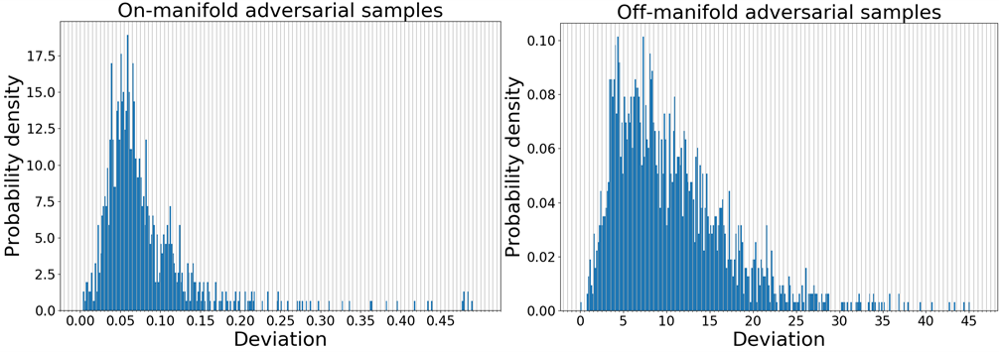
Figure 5: Deviation distributions of on/off-manifold adversarial samples (attacking STGCN) on HDM05 dataset.

TABLE IX: Comparisons. Top: STGCN, Middle: MSG3D, Bottom: SGN. ’SMART’ and ’CIASA’ are the attack success rate of SMART and CIASA. Acc is the classification accuracy, i.e. average accuracy on clean data. ST means standard training. GS means Gaussian Smoothing.

Methods	BASAR-NoMP			SMART		CIASA		Acc
	$l\uparrow$	$\Delta a\uparrow$	$\Delta B/B\uparrow$	@50	@200	@50	@200
ST	0.1	0.04	0.66%	95.75%	99.33%	97.99%	99.33%	87.2%
BASAR-MMAT	2.07	0.67	10.91%	47.54%	92.63%	48.75%	93.75%	91.2%
SMART-MMAT	5.98	2.56	47.98%	5.80%	31.47%	5.80%	33.40%	91.0%
GS($\sigma=0.01$)	0.61	0.20	4.13%	86.16%	99.11%	86.61%	99.33%	91.9%
GS($\sigma=0.1$)	2.80	1.16	19.72%	28.57%	84.15%	30.80%	87.05%	90.4%
ST	0.70	0.09	1.81%	92.96%	98.44%	93.54%	95.56%	94.4%
BASAR-MMAT	4.53	0.86	15.86%	77.23%	92.41%	70.76%	91.13%	95.9%
SMART-MMAT	9.26	3.09	61.39%	3.64%	16.14%	2.82%	15.12%	95.1%
GS($\sigma=0.01$)	2.16	0.67	11.09%	49.06%	97.50%	51.62%	97.69%	94.4%
GS($\sigma=0.1$)	6.90	2.59	48.08%	4.24%	35.94%	4.01%	39.11%	94.4%
ST	7.93	2.00	39.64%	29.24%	74.28%	26.56%	76.04%	94.1%
BASAR-MMAT	14.85	3.76	80.26%	20.31%	71.09%	22.10%	70.31%	94.7%
SMART-MMAT	3.01	0.73	11.71%	7.03%	49.21%	7.42%	51.95%	93.9%
GS($\sigma=0.01$)	6.13	1.10	19.10%	32.29%	90.63%	35.04%	91.52%	94.7%
GS($\sigma=0.1$)	12.87	3.07	64.18%	15.10%	64.84%	17.71%	73.44%	93.2%

Both BASAR-MMAT and SMART-MMAT can improve the robustness (Table IX) and SMART-MMAT has slightly better overall performance. This is understandable since SMART-MMAT is while-box and computes more aggressive adversaries. However, BASAR-MMAT can achieve better accuracy than standard training and SMART-MMAT, which show BASAR-MMAT can potentially eliminate the accuracy-robustness trade-off. Overall, MMAT is effective under both white-box and black-box samplers.

VI Discussion and Conclusion

We proposed the very first black-box adversarial attack method which gives strong performance across datasets, models and attack modes. Exhaustive qualitative and quantitative evaluations and comparisons show the superiority of the proposed method. More broadly, we show, for the first time, the wide existence of on-manifold adversarial samples in skeletal motions. Based on the attack, we discuss what classifiers tend to be robust against attack. We also proposed a new adversarial training method to achieve simultaneous improvement on accuracy and robustness in general.

One limitation is that BASAR relies on an explicit manifold parameterization which is not always feasible. This can be mitigated by learning from a large motion dataset and use the learned model to do the manifold projection, similar to [60]. Another limitation is we still need human-in-the-loop perceptual study to evaluate the quality of the attack. However, objective perceptual metrics regarding skeleton motions is still a research gap. Finally, BASAR adversarial samples can be theoretically realized by humans because they are on the natural manifold. However, how to attack a system in the real world using BASAR still depends on the specific setting of the system. In this research, we make the first step to identify the potential danger.

In future, we will investigate the perceptually-guided adversarial attack. We found that imperceptible perturbations form a small subspace of the adversarial samples, which intersects with both on-manifold and off-manifold samples. The interplay among the decision boundary, the data manifold and the imperceptible subspace will lead to adversarial samples with higher quality.

References

- [1] H. Wang, F. He, Z. Peng, Y.-L. Yang, T. Shao, K. Zhou, and D. Hogg, “Understanding the robustness of skeleton-based action recognition under adversarial attack,” in CVPR, 2021.
- [2] J. Gilmer, L. Metz, F. Faghri, S. S. Schoenholz, M. Raghu, M. Wattenberg, and I. Goodfellow, “Adversarial Spheres,” arXiv:1801.02774 [cs], 2018.
- [3] C. Szegedy, W. Zaremba, I. Sutskever, J. Bruna, D. Erhan, I. Goodfellow, and R. Fergus, “Intriguing properties of neural networks,” arXiv:1312.6199 [cs], 2014.
- [4] N. Akhtar and A. Mian, “Threat of adversarial attacks on deep learning in computer vision: A survey,” IEEE Access, vol. 6, pp. 14 410–14 430, 2018.
- [5] A. Chakraborty, M. Alam, V. Dey, A. Chattopadhyay, and D. Mukhopadhyay, “Adversarial Attacks and Defences: A Survey,” arXiv:1810.00069 [cs, stat], 2018.
- [6] F. Karim, S. Majumdar, and H. Darabi, “Adversarial attacks on time series,” IEEE Transactions on Pattern Analysis and Machine Intelligence, 2020.
- [7] H. I. Fawaz, G. Forestier, J. Weber, L. Idoumghar, and P.-A. Muller, “Adversarial attacks on deep neural networks for time series classification,” IEEE, pp. 1–8, 2019.
- [8] S. Harford, F. Karim, and H. Darabi, “Adversarial attacks on multivariate time series,” arXiv preprint arXiv:2004.00410, 2020.
- [9] B. Ren, M. Liu, R. Ding, and H. Liu, “A Survey on 3D Skeleton-Based Action Recognition Using Learning Method,” arXiv:2002.05907 [cs], 2020.
- [10] J. Liu, N. Akhtar, and A. Mian, “Adversarial attack on skeleton-based human action recognition,” IEEE Transactions on Neural Networks and Learning Systems, pp. 1–14, 2020.
- [11] T. Zheng, S. Liu, C. Chen, J. Yuan, B. Li, and K. Ren, “Towards Understanding the Adversarial Vulnerability of Skeleton-based Action Recognition,” arXiv:2005.07151 [cs], 2020.
- [12] F. Tramèr, N. Papernot, I. Goodfellow, D. Boneh, and P. McDaniel, “The Space of Transferable Adversarial Examples,” arXiv:1704.03453 [cs, stat], 2017.
- [13] D. Stutz, M. Hein, and B. Schiele, “Disentangling adversarial robustness and generalization,” CVPR, pp. 6969–6980, 2019.
- [14] D. Tsipras, S. Santurkar, L. Engstrom, A. Turner, and A. Madry, “Robustness may be at odds with accuracy,” in ICLR, 2019.
- [15] H. Zhang, Y. Yu, J. Jiao, E. P. Xing, L. E. Ghaoui, and M. I. Jordan, “Theoretically principled trade-off between robustness and accuracy,” in ICML, vol. 97, 2019, pp. 7472–7482.
- [16] D. Su, H. Zhang, H. Chen, J. Yi, P.-Y. Chen, and Y. Gao, “Is robustness the cost of accuracy?–a comprehensive study on the robustness of 18 deep image classification models,” in ECCV, 2018, pp. 631–648.
- [17] Y. Diao, T. Shao, Y.-L. Yang, K. Zhou, and H. Wang, “Basar:black-box attack on skeletal action recognition,” in CVPR, 2021.
- [18] R. Vemulapalli, F. Arrate, and R. Chellappa, “Human action recognition by representing 3d skeletons as points in a lie group,” in CVPR, 2014, pp. 588–595.
- [19] B. Fernando, E. Gavves, J. O. M., A. Ghodrati, and T. Tuytelaars, “Modeling video evolution for action recognition,” in CVPR, 2015, pp. 5378–5387.
- [20] Y. Du, W. Wang, and L. Wang, “Hierarchical recurrent neural network for skeleton based action recognition,” in CVPR, 2015, pp. 1110–1118.
- [21] J. Liu, A. Shahroudy, D. Xu, and G. Wang, “Spatio-temporal lstm with trust gates for 3d human action recognition,” in ECCV, 2016, pp. 816–833.
- [22] M. Liu, H. Liu, and C. Chen, “Enhanced skeleton visualization for view invariant human action recognition,” Pattern Recogn., vol. 68, no. C, pp. 346–362, 2017.
- [23] Q. Ke, M. Bennamoun, S. An, F. A. Sohel, and F. Boussaïd, “A new representation of skeleton sequences for 3d action recognition,” in CVPR, 2017, pp. 4570–4579.
- [24] S. Yan, Y. Xiong, and D. Lin, “Spatial temporal graph convolutional networks for skeleton-based action recognition,” in AAAI, 2018.
- [25] L. Shi, Y. Zhang, J. Cheng, and H. Lu, “Two-stream adaptive graph convolutional networks for skeleton-based action recognition,” in CVPR, 2019.
- [26] P. Zhang, C. Lan, W. Zeng, J. Xing, J. Xue, and N. Zheng, “Semantics-guided neural networks for efficient skeleton-based human action recognition,” in CVPR, 2020.
- [27] Z. Liu, H. Zhang, Z. Chen, Z. Wang, and W. Ouyang, “Disentangling and unifying graph convolutions for skeleton-based action recognition,” in CVPR, 2020.
- [28] L. Sun, Y. Dou, C. Yang, J. Wang, P. S. Yu, and B. Li, “Adversarial attack and defense on graph data: A survey,” arXiv preprint arXiv:1812.10528, 2018.
- [29] W. E. Zhang, Q. Z. Sheng, A. Alhazmi, and C. Li, “Adversarial attacks on deep-learning models in natural language processing: A survey,” ACM Transactions on Intelligent Systems and Technology, vol. 11, no. 3, pp. 1–41, 2020.
- [30] I. J. Goodfellow, J. Shlens, and C. Szegedy, “Explaining and harnessing adversarial examples,” ICLR, 2015.
- [31] A. Kurakin, I. Goodfellow, and S. Bengio, “Adversarial examples in the physical world,” ICLR Workshop, 2017.
- [32] N. Carlini and D. Wagner, “Towards evaluating the robustness of neural networks,” IEEE Symposium on Security and Privacy, 2017.
- [33] J. Hwang, J.-H. Kim, J.-H. Choi, and J.-S. Lee, “Just one moment: Structural vulnerability of deep action recognition against one frame attack,” in CVPR, 2021, pp. 7668–7676.
- [34] N. Papernot, P. D. McDaniel, and I. J. Goodfellow, “Transferability in machine learning: from phenomena to black-box attacks using adversarial samples,” CoRR, vol. abs/1605.07277, 2016.
- [35] P.-Y. Chen, H. Zhang, Y. Sharma, J. Yi, and C.-J. Hsieh, “Zoo: Zeroth order optimization based black-box attacks to deep neural networks without training substitute models,” in Proceedings of the 10th ACM Workshop on Artificial Intelligence and Security, 2017, pp. 15–26.
- [36] C. Tu, P. Ting, P. Chen, S. Liu, H. Zhang, J. Yi, C. Hsieh, and S. Cheng, “Autozoom: Autoencoder-based zeroth order optimization method for attacking black-box neural networks,” in AAAI, 2019, pp. 742–749.
- [37] W. Brendel, J. Rauber, and M. Bethge, “Decision-based adversarial attacks: Reliable attacks against black-box machine learning models,” in ICLR, 2018.
- [38] J. Chen, M. I. Jordan, and M. J. Wainwright, “Hopskipjumpattack: A query-efficient decision-based attack,” in IEEE Symposium on Security and Privacy (SP), 2020, pp. 1277–1294.
- [39] M. Cheng, S. Singh, P. H. Chen, P. Chen, S. Liu, and C. Hsieh, “Sign-opt: A query-efficient hard-label adversarial attack,” in ICLR, 2020.
- [40] M. Cheng, T. Le, P. Chen, H. Zhang, J. Yi, and C. Hsieh, “Query-efficient hard-label black-box attack: An optimization-based approach,” in ICLR, 2019.
- [41] H. Li, X. Xu, X. Zhang, S. Yang, and B. Li, “Qeba: Query-efficient boundary-based blackbox attack,” CVPR, pp. 1218–1227, 2020.
- [42] J. Chen and Q. Gu, “Rays: A ray searching method for hard-label adversarial attack,” in KDD ’20, 2020, pp. 1739–1747.
- [43] Z. Wei, J. Chen, X. Wei, L. Jiang, T. Chua, F. Zhou, and Y. Jiang, “Heuristic black-box adversarial attacks on video recognition models,” in AAAI, 2020, pp. 12 338–12 345.
- [44] X. Wei, H. Yan, and B. Li, “Sparse black-box video attack with reinforcement learning,” International Journal of Computer Vision, pp. 1–15, 2022.
- [45] L. Jiang, X. Ma, S. Chen, J. Bailey, and Y.-G. Jiang, “Black-box adversarial attacks on video recognition models,” in ACM MM, 2019, pp. 864–872.
- [46] S. Li, A. Aich, S. Zhu, S. Asif, C. Song, A. Roy-Chowdhury, and S. Krishnamurthy, “Adversarial attacks on black box video classifiers: Leveraging the power of geometric transformations,” NIPS, vol. 34, 2021.
- [47] A. Madry, A. Makelov, L. Schmidt, D. Tsipras, and A. Vladu, “Towards deep learning models resistant to adversarial attacks,” in ICLR, 2018.
- [48] E. Wong and J. Z. Kolter, “Provable defenses against adversarial examples via the convex outer adversarial polytope,” in ICML, vol. 80, 2018, pp. 5283–5292.
- [49] A. Raghunathan, J. Steinhardt, and P. Liang, “Certified defenses against adversarial examples,” in ICLR, 2018.
- [50] V. Tjeng, K. Y. Xiao, and R. Tedrake, “Evaluating robustness of neural networks with mixed integer programming,” in ICLR, 2019.
- [51] Y. Tsuzuku, I. Sato, and M. Sugiyama, “Lipschitz-margin training: scalable certification of perturbation invariance for deep neural networks,” in NeurIPS, 2018, pp. 6542–6551.
- [52] M. Lécuyer, V. Atlidakis, R. Geambasu, D. Hsu, and S. Jana, “Certified robustness to adversarial examples with differential privacy,” in 2019 IEEE Symposium on Security and Privacy, SP 2019. IEEE, 2019, pp. 656–672.
- [53] J. M. Cohen, E. Rosenfeld, and J. Z. Kolter, “Certified adversarial robustness via randomized smoothing,” in ICML, vol. 97, 2019, pp. 1310–1320.
- [54] F. Croce, M. Andriushchenko, V. Sehwag, N. Flammarion, M. Chiang, P. Mittal, and M. Hein, “Robustbench: a standardized adversarial robustness benchmark,” arXiv preprint arXiv:2010.09670, 2020.
- [55] T. Miyato, S. Maeda, M. Koyama, and S. Ishii, “Virtual adversarial training: A regularization method for supervised and semi-supervised learning,” IEEE Transactions on Pattern Analysis and Machine Intelligence, vol. 41, no. 8, pp. 1979–1993, 2019.
- [56] Y. Carmon, A. Raghunathan, L. Schmidt, J. C. Duchi, and P. Liang, “Unlabeled data improves adversarial robustness,” in NeurIPS, 2019, pp. 11 190–11 201.
- [57] A. Raghunathan, S. M. Xie, F. Yang, J. C. Duchi, and P. Liang, “Understanding and mitigating the tradeoff between robustness and accuracy,” in ICML, 2020.
- [58] D. Stutz, M. Hein, and B. Schiele, “Disentangling adversarial robustness and generalization,” in CVPR, 2019, pp. 6976–6987.
- [59] Y. Yang, C. Rashtchian, H. Zhang, R. R. Salakhutdinov, and K. Chaudhuri, “A closer look at accuracy vs. robustness,” in NeurIPS, 2020.
- [60] H. Wang, E. S. L. Ho, H. P. H. Shum, and Z. Zhu, “Spatio-temporal manifold learning for human motions via long-horizon modeling,” IEEE Transactions on Visualization and Computer Graphics, pp. 1–1, 2019.
- [61] H. Wang, K. A. Sidorov, P. Sandilands, and T. Komura, “Harmonic parameterization by electrostatics,” ACM Transactions on Graphics (TOG), vol. 32, no. 5, p. 155, 2013.
- [62] H. Wang, E. S. Ho, and T. Komura, “An energy-driven motion planning method for two distant postures,” IEEE transactions on visualization and computer graphics, vol. 21, no. 1, pp. 18–30, 2015.
- [63] W. Chen, H. Wang, Y. Yuan, T. Shao, and K. Zhou, “Dynamic future net: Diversified human motion generation,” in ACM MM, 2020.
- [64] J. D. Hedengren, R. A. Shishavan, K. M. Powell, and T. F. Edgar, “Nonlinear modeling, estimation and predictive control in apmonitor,” Computers & Chemical Engineering, vol. 70, pp. 133–148, 2014.
- [65] C. Xie, M. Tan, B. Gong, J. Wang, A. L. Yuille, and Q. V. Le, “Adversarial examples improve image recognition,” in CVPR, 2020, pp. 819–828.
- [66] M. Müller, T. Röder, M. Clausen, B. Eberhardt, B. Krüger, and A. Weber, “Documentation mocap database hdm05,” Universität Bonn, Tech. Rep. CG-2007-2, 2007.
- [67] A. Shahroudy, J. Liu, T.-T. Ng, and G. Wang, “Ntu rgb+ d: A large scale dataset for 3d human activity analysis,” in CVPR, 2016, pp. 1010–1019.
- [68] W. Kay, J. Carreira, K. Simonyan, B. Zhang, C. Hillier, S. Vijayanarasimhan, F. Viola, T. Green, T. Back, P. Natsev, M. Suleyman, and A. Zisserman, “The kinetics human action video dataset,” 2017.
- [69] T. Li, J. Liu, W. Zhang, Y. Ni, W. Wang, and Z. Li, “Uav-human: A large benchmark for human behavior understanding with unmanned aerial vehicles,” CVPR, pp. 16 261–16 270, 2021.
- [70] Z. Cao, T. Simon, S.-E. Wei, and Y. Sheikh, “Realtime multi-person 2d pose estimation using part affinity fields,” in CVPR, 2017, pp. 7291–7299.