An Optimal $k$ Nearest Neighbours Ensemble for Classification Based on Extended Neighbourhood Rule with Features subspace

Abstract

To minimize the effect of outliers, $k$NN ensembles identify a set of closest observations to a new sample point to estimate its unknown class by using majority voting in the labels of the training instances in the neighbourhood. Ordinary $k$NN based procedures determine $k$ closest training observations in the neighbourhood region (enclosed by a sphere) by using a distance formula. The $k$ nearest neighbours procedure may not work in a situation where sample points in the test data follow the pattern of the nearest observations that lie on a certain path not contained in the given sphere of nearest neighbours. Furthermore, these methods combine hundreds of base $k$NN learners and many of them might have high classification errors thereby resulting in poor ensembles. To overcome these problems, an optimal extended neighbourhood rule based ensemble is proposed where the neighbours are determined in $k$ steps. It starts from the first nearest sample point to the unseen observation. The second nearest data point is identified that is closest to the previously selected data point. This process is continued until the required number of the $k$ observations are obtained. Each base model in the ensemble is constructed on a bootstrap sample in conjunction with a random subset of features. After building a sufficiently large number of base models, the optimal models are then selected based on their performance on out-of-bag (OOB) data. The proposed ensemble is compared with other state-of-the-art procedures on 17 benchmark datasets. Performance metrics used for comparison are accuracy, Cohen’s kappa and Brier score (BS). The performance of the proposed method and other classical procedures are also assessed by adding contrived features to the given datasets. For further assessment of the methods, boxplots of the results are also constructed. The results reveal that the proposed method outperforms the other methods in most of the cases.

I Introduction

Classification is a supervised learning problem dealing with the prediction of categorical response values for unseen observations using a set of independent features according to training data. $k$ nearest neighbours ($k$NN) is one of the top-ranked procedures used for classification learning problems [1, 2, 3, 4]. It is a simple, easy to understand and non-parametric procedure which gives effective results in many cases, especially in large datasets [5, 6, 7, 8]. The $k$NN procedure determines $k$ nearest observations in the neighbourhood of a test point using a distance formula and predicts its class by using majority voting. As the $k$NN method is simple, easy and outperforms other complex classifiers in many cases, however, $k$NN is affected by many data-related problems, such as noise and irrelevant features in the data.

To improve the classification accuracy of the $k$NN based classifiers, various ensemble procedures have been proposed. For example, bootstrap aggregated $k$NN [9], ensemble of subset of $k$NN [10], random $k$NN [11], weighted heterogeneous distance Metric [12], optimal $k$NN ensemble [13], ensemble of random subspace $k$NN [14], etc. These methods try to make the base $k$NN learners more diverse and accurate to reduce the chance of the same errors repetition [15, 16, 17, 18]. Almost all these techniques use majority voting based on the response values of the observations in the neighbourhood of the unseen sample point. To estimate the final prediction of the query point, the second round of majority voting is used based on the results given by the base learners. However, the prediction accuracy of these methods might be affected in the case of datasets with a majority of features as irrelevant and/or observations outside the general pattern of the data. This increases the likelihood of the ensemble being adversely affected by the noisy features and/or outliers. Therefore, modifying the nearest neighbourhood rule and selecting optimal models in such situations are needed to maintain the prediction accuracy. Several studies in literature are devoted to model selection for ensemble creation [19, 20, 21, 22, 10, 23, 24]. Similarly, to mitigate the effect of an outlier on the nearest neighbours, several studies have proposed modified neighbourhood identification methods. Examples of such procedures could be found in [25, 26, 27, 28, 29, 30, 31, 32].

The current paper proposes an optimal ensemble procedure using the extended neighbourhood rule (ExNRule) for $k$NN [33] as a merger of modified neighbourhood identification and model selection. The method is named optimal extended neighbourhood rule ensemble (OExNRule). A large number of base ExNRule models are constructed each on a bootstrap sample with a subset of features and the error rate of each model is computed on out-of-bag (OOB) data points. After building a large number of $k$NN models via the ExNRule, the proportion of best performing models is selected based on their OOB errors as the final ensemble. To assess the performance of the proposed procedure, 17 benchmark datasets are considered using classification accuracy, Cohen’s kappa and Brier score (BS) as performance metrics. The performance is compared with state-of-the-art procedures i.e. $k$ nearest neighbour ($k$NN), weighted $k$ nearest neighbours (W$k$NN), random $k$ nearest neighbour (R$k$NN), random forest (RF), optimal trees ensemble (OTE) and support vector machine (SVM). Boxplots have also been constructed for further assessment of the results of the proposed OExNRule and the other competitors. The rest of the article is organized as follows:

The related literature is summarized in Section II. The suggested procedure, its algorithm and mathematical description are given in Section III. Experimental setup, detailed discussion on results and the considered datasets with additional contrived features are given in Section IV. Section V, summarize the paper with concluding remarks.

II Related works

Various $k$NN based procedures have been proposed to improve the performance of the classical $k$NN algorithm. As observations in the neighbourhood of a test point determined by the classical $k$NN procedure have equal weights, Bailey et al. [34] suggested a weighted $k$ nearest neighbours (W$k$NN) technique based on the distance computed from the test observation to the nearest neighbours. This method improves the performance of the base $k$NN in many cases. However, W$k$NN is a global procedure as it utilizes all the training samples which makes the method time-consuming. To overcome this problem, others have proposed condensed nearest neighbour (CNN) procedures such as methods given in [35, 36, 37]. These methods remove similar data points as they do not add valuable information. Although the CNN procedures boost the query time, there is a possibility to ignore training observations on the boundary as they depend on the order of the dataset. Like the CNN methods, Gyeoffrey et al. [38] suggested a procedure by ignoring those instances which do not affect the results known as a reduced nearest neighbour (RNN). This procedure removes templates and reduces the data in the training part. However, like the CNN method, the RNN procedure is computationally complex. For further improvement, a model based $k$NN procedure is proposed by Guo et al. [39]. This method uses a function fitted to the training part of the data to predict unseen observations. Like CNN and RNN, this technique also reduces the size of the training data and gives promising results. However, this procedure ignores the marginal observations which lie beyond the region. A more robust procedure called clustered $k$NN is proposed in [40], to overcome the problem of uneven distribution of observations in training data. This method selects the instances in the neighbourhood from the clusters. Threshold selection used in this method to calculate distances among sample points within clusters is a difficult task and optimization of $k$ value for each class is also unknown. Parvin et al. [41] suggested a modified $k$ nearest neighbour (M$k$NN) procedure using weights and validity of the observations to predict an unseen sample point. Carlotta et al. [42] proposed a locally adaptive nearest neighbour classifier for bias reduction known as adaptive metric nearest neighbor algorithm (ADAMENN). Authors have used a Chi-squared distance analysis to calculate a flexible/pliable metric for determining nearest neighbours that are more adaptive to the location of the test point. ADAMENN selects those nearest observations which exhort more importance to the more relevant features as compared to the irrelevant features. Sproull [43] proposed a $k$ dimensional tree nearest neighbour ($k$DTNN) technique. This method divides the training observations into half planes to organize the multi-dimensional instances. $k$dNN algorithm produces a balance tree and is simple to understand. However, it needs intensive search and slices the data samples into half blindly. Furthermore, it is computationally complex and might miss the structure of the data. Authors in [44] constructed a hybrid technique based on support vector machine (SVM) and $k$NN procedures. Further improvements in the $k$NN based techniques can be seen in [45, 46, 47, 48, 49, 50].

In addition to the above studies, there are several $k$NN based ensemble techniques proposed to improve the model accuracy and make the models more diverse. Breiman in [51] suggested a bootstrap aggregation (or simply bagging) procedure, it is one of the basic ensemble methods and develops a novel model to estimate the exact bootstrap average in the long run of the model [52, 53, 54]. Bagging is the fundamental block of many classical ensemble procedures. Methods based on the bagging technique draw a large number of random bootstrap samples of the same size and construct a base classifier on each sample. The final estimated class of a test point is the majority vote in the results given by all base learners [51]. The exact bagging technique is further extended by Steel [9] to sub-sampling with and without replacement aggregation. Several ensemble procedures have been proposed that use bagging and features subsets for constructing base $k$NN learners [55, 11, 10, 56]. Moreover, [57, 49] have proposed $k$ value optimization in base $k$NN classifiers to construct ensemble methods. The idea of boosting $k$NN is given by Pedrajas and Boyer [18], it is a combination of two methodologies to improve the performance of the ensemble. The first methodology is based on feature subset while the second is based on the transformation of the feature space using a non-linear projection. Other studies can be seen in [58, 59, 60, 61, 62, 63] to boost up the $k$NN procedure and get improved results.

Ensemble procedures have a large number of base models, therefore, they are computationally complex and time-consuming. To reduce this issue, several authors have proposed algorithms such as the ensemble of a subset of $k$NN models (ES$k$NN) [10] for model selection. It is an ensemble procedure based on optimal models selected based on out-of-bag errors. It gives efficient results particularly in the case of datasets which have non-informative features. Further examples of similar procedures can be found in [19, 20, 21, 22, 24, 64]. Although these procedures have shown promising results in many situations. However, they might give poor results due to mixed patterns in the data. Therefore, these methods need further improvement.

This paper proposes an optimal extended neighbourhood rule (OExNRule) for $k$NN ensemble. This method takes a large number $B$ bootstrap samples from training data at first stage, each with a subsets of features. The method applies ExNRule [33] on each bootstrap sample and compute out-of-bag (OOB) error. It then orders the models based on the OOB errors given by all $B$ models and selects a proportion of top ranked ExNRule learners with minimum OOB errors. Final ensemble is constructed by combining the selected models to predict the test data. This procedure improves the performance in the following ways.

1. The $k$ nearest instances are chosen in a step-wise manner to determine the true representative pattern of the unseen observation in the training data.

2. The base models are diverse as each model fitted on a random bootstrap sample in conjunction with a random subset of features for each model. Furthermore, it also avoids over-fitting.

3. To ensure accuracy for the base learners, models are selected from a large number $B$ ExNRule learners [33] on the basis of their OOB errors.

III The Optimal Extended Neighbourhood Rule (OExNRule) for $k$NN Ensemble

Suppose a training dataset $\mathcal{L}=(X,Y)_{n\times(p+1)}$, where $X_{n\times p}$ is feature space with $n$ observations and $p$ features and $Y$ is a binary response variable i.e. $Y\in(0,1)$. Let $B$ random bootstrap sample of size $n$ with replacement are taken from the training data $\mathcal{L}$ and a random sub-sample without replacement of $p^{\prime}\leq p$ features with each bootstrap sample is also drawn i.e. $S_{n\times(p^{\prime}+1)}^{b}$, where, $b=1,2,3,\ldots,B$. Then apply ExNRule [33] on each bootstrap sample i.e. $S_{n\times(p^{\prime}+1)}^{b}$ and compute out-of-bag (OOB) errors i.e. $E^{b}$, where, $b=1,2,3,\ldots,B$. Rank the models with respect to the OOB errors $E^{b}$s in ascending order and choose a proportion of the top ranked $B^{\prime}$ models. Based on the selected models, determine the predictions of an unseen observation by all $B^{\prime}$ ExNRule models i.e. $\hat{Y}^{1},\hat{Y}^{2},\hat{Y}^{3},\ldots,\hat{Y}^{B^{\prime}}$. The final estimated class of the unseen observation is the majority vote of the predictions given by the top ranked $B^{\prime}$ models.

III-A Mathematical Description of the Optimal Extended Neighbourhood Rule

Extended neighbourhood rule [33] determines $k$ nearest observations in a sequence to a test point $X_{1\times p^{\prime}}^{0}$ in $b^{th}$ bootstrap sample using a distance formula as follows:

$$\delta_{b}(X_{1\times p^{\prime}}^{i-1},X_{1\times p^{\prime}}^{i})_{min}=\left[\sum_{j=1}^{p^{\prime}}|x_{j}^{i-1}-x_{j}^{i}|^{q}\right]^{1/q},$$ (1)

$$\text{where, }i=1,2,\ldots,k\text{ and }b=1,2,\ldots,B.$$

Equation 1 gives the required sequence of the distances as bellows:

$$\delta_{b}(X_{1\times p^{\prime}}^{0},X_{1\times p^{\prime}}^{1})_{min},\delta_{b}(X_{1\times p^{\prime}}^{1},X_{1\times p^{\prime}}^{2})_{min},$$

$$\delta_{b}(X_{1\times p^{\prime}}^{2},X_{1\times p^{\prime}}^{3})_{min},\ldots,\delta_{b}(X_{1\times p^{\prime}}^{k-1},X_{1\times p^{\prime}}^{k})_{min}.$$

The above sequence indicates that, the nearest data point to $X_{1\times p^{\prime}}^{i-1}$ is $X_{1\times p^{\prime}}^{i}$, where, $i=1,2,3,\ldots,k$. This gives the required $k$ observations in the pattern i.e. $X_{1\times p^{\prime}}^{1},X_{1\times p^{\prime}}^{2},X_{1\times p^{\prime}}^{3},\ldots,X_{1\times p^{\prime}}^{k}$ and their corresponding classes are $y^{1},y^{2},y^{3},\ldots,y^{k}$ respectively. The estimated class label of $X_{1\times p}^{0}$ from the $b^{th}$ learner is determine by the majority voting i.e.

$$\hat{Y}^{b}=\text{majority vote of }(y^{1},y^{2},y^{3},\ldots,y^{k}),$$

The $b^{th}$ base model $H^{b}(.)$, uses the above rule to compute the out-of-bag error $E^{b}$. In this way, a total of $B$ base models are constructed and their out-of-bag errors are also computed. These models are ranked in ascending order according to their performance i.e. $H^{1}(.),H^{2}(.),H^{3}(.),\ldots,H^{B}(.)$. A proportion of top ranked $B^{\prime}$ models is selected i.e. $H^{1}(.),H^{2}(.),H^{3}(.),\ldots,H^{B^{\prime}}(.)$, which comprise the final ensemble to predict the test data.

III-B Algorithm

The proposed OExNRule based ensemble takes the following steps.

1. Draw $B$ random bootstrap samples from training observations in conjunction with a random subset of $p^{\prime}<p$ features without replacement.

2. Using ExNRule [33] in each sample drawn in Step 1 to construct base models.

3. Compute out-of-bag (OOB) errors $E^{b}$ for each base model constructed in Step 2.

4. Rank the models according to their OOB errors $E^{b}$ in ascending order.

5. Select $B^{\prime}$ models based on the individual $E^{b}$ values and combine them in an ensemble.

6. Use the ensemble formed in Step 5 for prediction purposes.

Algorithm 1 shows the pseudo code of the proposed OExNRule procedure and an illustrating flow chart of the method given in Figure 1.

Algorithm 1 Pseudo code of the proposed OExNRule.

1:  $\mathcal{L}=(X,Y)_{n\times(p+1)}$ $\leftarrow$ Training dataset with dimension $n\times(p+1)$;

2:  $X_{n\times p}$ $\leftarrow$ Training feature space with dimension $n\times p$;

3:  $Y$ $\leftarrow$ Vector of $n$ response values of training data;

4:  $p$ $\leftarrow$ Total number of features in the training data;

5:  $n$ $\leftarrow$ Total number of observations in training data;

6:  $B$ $\leftarrow$ Number of bootstrap samples each with dimension $n\times(p^{\prime}+1)$;

7:  $B^{\prime}$ $\leftarrow$ Number of top ranked models according to the individual performance;

8:  $p^{\prime}$ $\leftarrow$ Size of the random subset of features taken with each bootstrap sample;

9:  $k$ $\leftarrow$ Number of data points to determine for a test point in $k$ steps;

10:  for $b\leftarrow 1:B$ do

11:     $S_{n\times(p^{\prime}+1)}^{b}$ $\leftarrow$ Bootstrap sample with dimension $n\times p^{\prime}$ taken from $X_{n\times p}$;

12:     $OH^{b}(.)$ $\leftarrow$ Construct a $k$NN model using ExNRule [33] on $S_{n\times(p^{\prime}+1)}^{b}$;

13:     $E^{b}$ $\leftarrow$ Error rate on out-of-bag observations computed by $OH^{b}(.)$;

14:  end for

15:  $OH^{b}(.)$ $\leftarrow$ Rank the $B$ models according to the individual performance in ascending order;

16:  Select $B^{\prime}$ top ranked models based on their individual performance;

17:  Use it as the final ensemble;

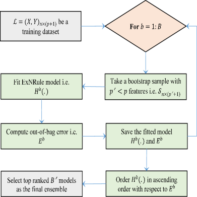
Figure 1: Flow chart of the proposed optimal extended neighbourhood rule (OExNRule) ensemble.

IV Experiments and results

This section describes the benchmark datasets and experimental setup of the analysis as given in the following subsections.

IV-A Benchmark datasets

IV-A1 Benchmark datasets with original features

For assessing the performance of the proposed model against the other standard procedures, 17 benchmark datasets (downloaded from various openly accessed repositories) are used. A short summary of these datasets is presented in Table I, showing the data ID, name, number of features $p$, number of observations $n$, class wise distribution (+/-) and source of the datasets.

TABLE I: This table describes the characteristics of the benchmark datasets used in this paper.

ID	Data	p	n	$+/-$	Sources
A	ILPD	10	583	(167, 415)	https://www.openml.org/d/1480
B	Heart	13	303	(99, 204)	[65]
C	EMon	9	130	(64, 66)	https://www.openml.org/d/944
D	AR5	29	36	(8, 28)	https://www.openml.org/d/1062
E	Cleve	13	303	(138, 165)	https://www.openml.org/d/40710
F	BTum	9	286	(120, 166)	https://www.openml.org/d/844
G	Wisc	32	194	(90, 104)	https://www.openml.org/d/753
H	MC2	39	161	(52, 109)	https://www.openml.org/d/1054
I	PRel	12	182	(52, 130)	https://www.openml.org/d/1490
J	Sonar	60	208	(97, 111)	https://www.openml.org/d/40
K	Sleep	7	62	(29, 33)	https://www.openml.org/d/739
L	TSVM	80	156	(102, 54)	https://www.openml.org/d/41976
M	JEdit	8	369	(204, 165)	https://www.openml.org/d/1048
N	GDam	8	155	(49, 106)	https://www.openml.org/d/1026
O	CVine	8	52	(24, 28)	https://www.openml.org/d/815
P	PLRL	13	315	(182, 133)	https://www.openml.org/d/915
Q	KC1B	86	145	(60, 85)	https://www.openml.org/d/1066

IV-A2 Benchmark datasets with contrived features

For further assessment of the proposed OExNRule based ensemble and classical $k$NN based classifiers, the original datasets are contaminated by adding contrived features synthetically. The number of contrived features is equal to the actual number of features in the original datasets. These features are generated from the uniform distribution over the interval $[0,1]$.

IV-B Experimental setup

The experimental setup based on 17 benchmark datasets given in Table I is designed as follows. Each dataset is divided randomly into two non-overlapping parts, i.e. 70% training and 30% testing of the total observations in the dataset. This splitting criterion is repeated 500 times for each dataset. The proposed OExNRule and other state-of-the-art competitors i.e. $k$NN, Weighted $k$NN, Random $k$NN, random forest (RF), optimal trees ensemble (OTE) and support vector machine (SVM) are trained on the training part and tested on the testing part. Final results are given in Tables II-IV, which are obtained by averaging all the results of 500 splittings.

The proposed method is used with $B=500$ base models each on $p^{\prime}=\sqrt{p}$ features, $k=3$ nearest steps determined by Euclidean distance and a proportion (25%) of $B$ models are selected based on out-of-bag (OOB) errors $E^{b}$ i.e. $B^{\prime}$ models. Pooling the results of these models is done by using majority voting. For further assessment of the proposed method against standard $k$NN based procedures, the values of $k=3,5\text{and }7$ are used. The novel procedure is also compared with $k$NN based methods on the contaminated datasets by adding contrived/irrelevant features.

The R package caret [66] is used to train the $k$NN model, while package kknn [67] is used for the implementation of W$k$NN. The R package rknn [68] is used to fit R$k$NN classifier. For random forest (RF) and optimal trees ensemble (OTE), the R packages randomForest [69] and OTE [70] are used, respectively. For support vector machine (SVM), the R package kernlab [71] is used. Furthermore, to tune the hyper-parameter $k$, the R function tune.knn in package e1071 [72] is used. For R$k$NN different hyper-parameters are tuned manually in the R package rknn [68]. R function tune.randomForest is used to tune nodesize, ntree and mtry in the R package e1071 [72]. The same procedure is used to tune the parameters for the OTE method. The R library kernlab [71] is used for SVM with linear kernel and default parameter values.

IV-C Results

Table II shows that the novel OExNRule method has outperformed the other state-of-the-art procedures in the majority of the cases. The proposed OExNRule is giving optimal accuracy as compared to the other classical procedures on 10 datasets and gives similar results to R$k$NN on 2 datasets. $k$NN outperforms on 1 dataset, while W$k$NN does not give satisfactory results on any dataset. R$k$NN gives maximum accuracy on 2 datasets, while RF and OTE do not outperform the rest of the procedures on any of the datasets. SVM gives maximum accuracy on 2 datasets as compared to the other procedures.

In terms of Cohen’s kappa, the proposed OExNRule gives optimal results on 10 datasets, while the $k$NN procedure does not give better results on any of the datasets. W$k$NN outperformed the others on 2 datasets, while R$k$NN and RF give optimal performance in terms of kappa each on 1-1 dataset. OTE does not win on any dataset, while SVM outperformed the others on 3 datasets. Similarly, the proposed OExNRule outperformed all the other classical procedures on the Brier score (BS) metric. For further assessment, boxplots are also constructed and are given in Figures 2-4. The plots reveal that the proposed method has outperformed the rest of the procedures in the majority of the cases.

For assessing the performance of the proposed OExNRule and other $k$NN based methods using different $k$ values (i.e. $k=3,5$ and $7$). Table III shows results for 5 datasets regarding different $k$ values. It reveals that the proposed algorithm has outperformed the other procedures in the majority of the cases and is not affected by the $k$ value. Moreover, boxplots are also given in Figures 5-7. A similar conclusion could be drawn from the plots.

For further assessment, contrived/irrelevant features are added to the given datasets and the results are given in Table IV. It is clear from the table that OExNRule is robust to the problem of non-informative/irrelevant features in the datasets. The proposed method outperformed the rest of the methods in the majority of the cases. Furthermore, Figures 8-10 shows the boxplots of the results of the datasets with contrived features.

V Conclusion

The method proposed in this paper selects a proportion of optimal extended neighbourhood rule (ExNRule) based models using out-of-bag (OOB) error from a total of $B$ learners. The selected base ExNRule models are combined to predict the class labels of test data using majority voting. The results given in the paper suggest that the proposed method outperforms the other classical procedures and demonstrates high prediction accuracy when data have irrelevant features.

Furthermore, each ExNRule based model is constructed on a random bootstrap sample in conjunction with a random subset of features, showing diversity in the ensemble. The proposed method ensures high prediction performance due to randomization, selection of neighbours in $k$ steps pattern and model selection based on OOB error.

The performance of the proposed procedure could further be improved by using a proper distance formula and weighting schemes for choosing the nearest neighbours. Moreover, improvement in the performance can be maximized by using the feature selection methods as given in [73, 74, 75, 76, 77, 78, 79] during base model construction. These methods select top ranked features from the features space in the dataset and use them to fit the base learners.

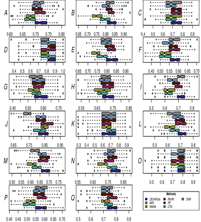
Figure 2: This figure shows the accuracy of the OExNRule and the other state-of-the-art procedures on the benchmark datasets in their original form.

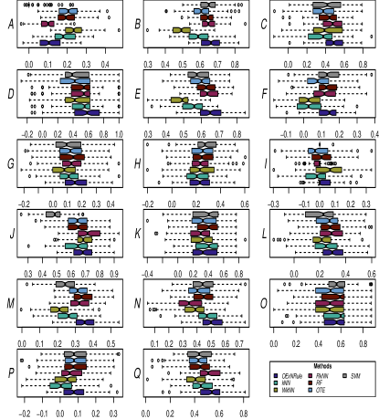
Figure 3: This figure shows the Cohen’s kappa of the OExNRule and the other state-of-the-art procedures on the benchmark datasets in their original form.

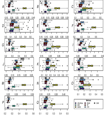
Figure 4: This figure shows the Brier score (BS) of the OExNRule and the other state-of-the-art procedures on the benchmark datasets in their original form.

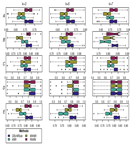
Figure 5: This figure shows the accuracy of the OExNRule and the other $k$NN based competitive procedures on the benchmark datasets in their original form using $k=3,5$ and $7$.

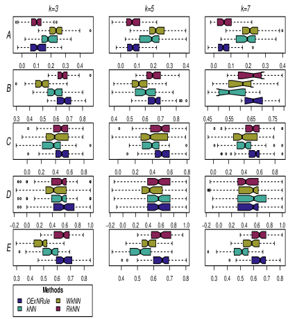
Figure 6: This figure shows the Cohen’s kappa of the OExNRule and the other $k$NN based competitive procedures on the benchmark datasets in their original form using $k=3,5$ and $7$.

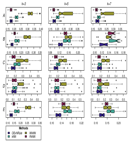
Figure 7: This figure shows the Brier score of the OExNRule and the other $k$NN based competitive procedures on the benchmark datasets in their original form using $k=3,5$ and $7$.

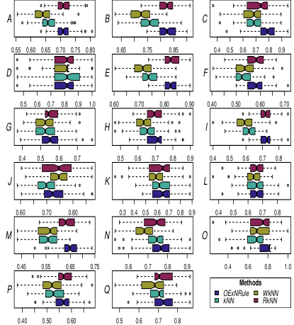
Figure 8: This figure shows the accuracy of the OExNRule and the other $k$NN based competitive procedures on the benchmark dataset with contrived features.

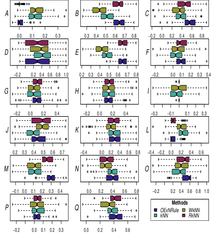
Figure 9: This figure shows the Cohen’s kappa of the OExNRule and the other $k$NN based competitive procedures on the benchmark dataset with contrived features.

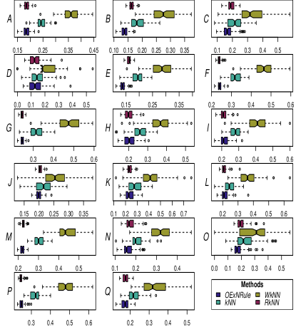
Figure 10: This figure shows the Brier score (BS) of the OExNRule and the other $k$NN based competitive procedures on the benchmark dataset with contrived features.

TABLE II: This table shows the accuracy, Cohen’s kappa and Brier score (BS) of the OExNRule and the other state-of-the-art procedures on the benchmark datasets in their original form.

Metrics	Methods	Datasets																	Mean
		$A$	$B$	$C$	$D$	$E$	$F$	$G$	$H$	$I$	$J$	$K$	$L$	$M$	$N$	$O$	$P$	$Q$
Accuracy	OExNRule	0.717	0.835	0.746	0.838	0.827	0.581	0.581	0.716	0.711	0.846	0.665	0.709	0.678	0.793	0.775	0.583	0.767	0.728
	$k$NN	0.678	0.798	0.677	0.821	0.776	0.525	0.556	0.677	0.625	0.820	0.680	0.651	0.632	0.772	0.782	0.515	0.742	0.690
	W$k$NN	0.682	0.750	0.707	0.789	0.745	0.530	0.538	0.686	0.623	0.850	0.661	0.622	0.608	0.720	0.756	0.521	0.709	0.676
	R$k$NN	0.717	0.828	0.732	0.826	0.823	0.577	0.568	0.716	0.700	0.864	0.645	0.697	0.667	0.751	0.750	0.584	0.764	0.718
	RF	0.707	0.825	0.711	0.824	0.814	0.571	0.570	0.712	0.681	0.824	0.679	0.694	0.676	0.769	0.779	0.570	0.723	0.713
	OTE	0.703	0.808	0.693	0.790	0.801	0.544	0.565	0.701	0.653	0.824	0.652	0.681	0.664	0.749	0.763	0.567	0.716	0.698
	SVM	0.710	0.828	0.698	0.782	0.793	0.577	0.551	0.706	0.713	0.740	0.679	0.643	0.623	0.772	0.786	0.580	0.734	0.701
Kappa	OExNRule	0.111	0.665	0.490	0.558	0.647	0.139	0.158	0.229	0.019	0.686	0.340	0.300	0.351	0.502	0.547	0.082	0.526	0.374
	$k$NN	0.186	0.591	0.355	0.516	0.550	0.027	0.113	0.202	-0.026	0.635	0.363	0.248	0.253	0.471	0.559	0.001	0.465	0.324
	W$k$NN	0.238	0.494	0.412	0.437	0.483	0.035	0.076	0.241	0.063	0.695	0.322	0.207	0.211	0.374	0.504	0.033	0.406	0.308
	R$k$NN	0.100	0.651	0.466	0.503	0.638	0.120	0.132	0.236	-0.014	0.724	0.298	0.284	0.325	0.349	0.500	0.067	0.520	0.347
	RF	0.195	0.645	0.422	0.493	0.623	0.128	0.136	0.254	0.009	0.644	0.369	0.289	0.344	0.447	0.552	0.081	0.440	0.357
	OTE	0.207	0.610	0.386	0.394	0.597	0.075	0.124	0.253	-0.014	0.643	0.315	0.261	0.318	0.410	0.518	0.081	0.429	0.330
	SVM	0.018	0.650	0.397	0.415	0.580	0.137	0.101	0.280	0.001	0.477	0.363	0.212	0.241	0.447	0.564	0.083	0.447	0.318
BS	OExNRule	0.177	0.125	0.178	0.119	0.127	0.255	0.254	0.200	0.226	0.118	0.228	0.198	0.207	0.155	0.164	0.242	0.173	0.185
	$k$NN	0.218	0.167	0.227	0.132	0.172	0.317	0.308	0.237	0.278	0.131	0.243	0.244	0.266	0.186	0.151	0.324	0.186	0.223
	W$k$NN	0.318	0.250	0.293	0.211	0.255	0.470	0.462	0.314	0.377	0.150	0.339	0.378	0.392	0.280	0.244	0.479	0.291	0.324
	R$k$NN	0.176	0.147	0.179	0.122	0.148	0.254	0.252	0.195	0.225	0.123	0.230	0.198	0.215	0.164	0.172	0.239	0.171	0.189
	RF	0.178	0.127	0.186	0.124	0.132	0.274	0.254	0.196	0.238	0.134	0.227	0.190	0.211	0.166	0.157	0.247	0.179	0.189
	OTE	0.183	0.133	0.206	0.185	0.138	0.311	0.262	0.206	0.248	0.129	0.258	0.198	0.222	0.181	0.178	0.255	0.187	0.205
	SVM	0.200	0.128	0.221	0.153	0.148	0.239	0.251	0.197	0.208	0.178	0.242	0.216	0.226	0.165	0.165	0.245	0.193	0.199

TABLE III: This table shows the accuracy, Cohen’s kappa and Brier score (BS) of the OExNRule and the other $k$NN based competitive procedures on the benchmark datasets in their original form using $k=3,5$ and $7$.

Metrics	Methods	Datasets															Mean
		$A$			$B$			$C$			$D$			$E$
		$k=3$	$k=5$	$k=7$	$k=3$	$k=5$	$k=7$	$k=3$	$k=5$	$k=7$	$k=3$	$k=5$	$k=7$	$k=3$	$k=5$	$k=7$
Accuracy	OEXNRule	0.717	0.716	0.717	0.835	0.833	0.838	0.746	0.761	0.767	0.838	0.825	0.813	0.827	0.826	0.826	0.792
	$k$NN	0.678	0.689	0.699	0.798	0.801	0.784	0.677	0.693	0.702	0.821	0.835	0.826	0.776	0.761	0.752	0.753
	W$k$NN	0.682	0.683	0.683	0.750	0.786	0.808	0.707	0.702	0.700	0.789	0.789	0.800	0.745	0.787	0.794	0.747
	R$k$NN	0.717	0.717	0.717	0.828	0.831	0.826	0.731	0.749	0.756	0.827	0.826	0.814	0.822	0.826	0.825	0.787
Kappa	OEXNRule	0.111	0.078	0.060	0.665	0.661	0.671	0.490	0.519	0.534	0.558	0.531	0.484	0.647	0.646	0.646	0.487
	$k$NN	0.186	0.184	0.194	0.591	0.598	0.564	0.355	0.387	0.409	0.516	0.531	0.498	0.550	0.520	0.500	0.439
	W$k$NN	0.238	0.221	0.215	0.494	0.567	0.610	0.412	0.404	0.401	0.437	0.437	0.457	0.483	0.571	0.584	0.435
	R$k$NN	0.100	0.076	0.063	0.651	0.658	0.649	0.463	0.503	0.519	0.511	0.512	0.461	0.638	0.645	0.645	0.473
BS	OEXNRule	0.177	0.180	0.184	0.125	0.124	0.124	0.178	0.180	0.185	0.119	0.120	0.125	0.127	0.127	0.128	0.147
	$k$NN	0.218	0.203	0.193	0.167	0.152	0.149	0.227	0.207	0.193	0.132	0.121	0.121	0.172	0.164	0.165	0.172
	W$k$NN	0.318	0.258	0.250	0.250	0.158	0.140	0.293	0.277	0.270	0.211	0.211	0.185	0.255	0.157	0.150	0.226
	R$k$NN	0.176	0.176	0.177	0.147	0.146	0.148	0.180	0.178	0.179	0.122	0.121	0.123	0.148	0.148	0.148	0.154

TABLE IV: This table shows the accuracy, Cohen’s kappa and Brier score (BS) of the OExNRule and the other $k$NN based competitive procedures on the benchmark datasets with contrived features.

Metrics	Methods	Datasets																	Mean
		$A$	$B$	$C$	$D$	$E$	$F$	$G$	$H$	$I$	$J$	$K$	$L$	$M$	$N$	$O$	$P$	$Q$
Accuracy	OExNRule	0.711	0.826	0.764	0.777	0.829	0.580	0.551	0.704	0.717	0.728	0.634	0.656	0.650	0.763	0.762	0.565	0.725	0.702
	$k$NN	0.659	0.760	0.693	0.801	0.740	0.528	0.527	0.653	0.616	0.702	0.621	0.655	0.560	0.738	0.677	0.531	0.700	0.657
	W$k$NN	0.640	0.722	0.665	0.769	0.712	0.538	0.527	0.635	0.592	0.748	0.599	0.626	0.555	0.682	0.704	0.521	0.669	0.641
	R$k$NN	0.711	0.820	0.716	0.785	0.827	0.581	0.555	0.704	0.716	0.745	0.614	0.658	0.634	0.738	0.716	0.571	0.725	0.695
Kappa	OExNRule	0.013	0.645	0.531	0.304	0.652	0.091	0.103	0.152	0.000	0.450	0.286	0.047	0.291	0.397	0.524	0.031	0.427	0.291
	$k$NN	0.125	0.513	0.387	0.422	0.474	0.035	0.054	0.141	-0.029	0.397	0.252	0.240	0.113	0.385	0.352	0.038	0.380	0.252
	W$k$NN	0.132	0.437	0.330	0.353	0.418	0.059	0.056	0.141	0.000	0.488	0.206	0.205	0.107	0.280	0.402	0.028	0.313	0.233
	R$k$NN	0.002	0.631	0.447	0.325	0.647	0.086	0.109	0.157	-0.001	0.484	0.251	0.059	0.256	0.302	0.440	0.038	0.427	0.274
BS	OExNRule	0.185	0.138	0.172	0.135	0.137	0.241	0.246	0.205	0.216	0.199	0.236	0.215	0.220	0.163	0.178	0.249	0.173	0.195
	$k$NN	0.243	0.182	0.215	0.146	0.193	0.321	0.317	0.259	0.280	0.214	0.282	0.245	0.302	0.204	0.232	0.320	0.218	0.245
	W$k$NN	0.360	0.278	0.335	0.231	0.288	0.462	0.473	0.365	0.408	0.252	0.401	0.374	0.445	0.318	0.296	0.479	0.331	0.359
	R$k$NN	0.185	0.162	0.191	0.131	0.162	0.239	0.245	0.201	0.213	0.204	0.234	0.210	0.226	0.174	0.197	0.246	0.175	0.200

Amjad Ali received the bachelor’s degree in statistics, the master’s in statistics from University of Peshawar, Pakistan, in 2014 and 2017, respectively. He is pursuing the Ph.D. degree with the Department of Statistics, Abdul Wali Khan University Mardan, Pakistan. His focus is on linear models, machine learning, applied statistics, causal inference, and computational statistics.

Muhammad Hamraz received the bachelor’s degree in statistics, the master’s and M. Phil. degrees in statistics from Quaid Azam University Islamabad, Pakistan, in 2004, 2007 and 2010 respectively. He is an Assistant Professor of statistics with Abdul Wali Khan University Mardan, Pakistan. His focus is on linear models, biostatics, applied statistics, and computational statistics.

Dost Muhammad Khan received the bachelor’s degree in statistics, the master’s and Ph.D. degrees in statistics from the University of Peshawar, Pakistan, in 2000, 2003, and 2012, respectively. He is an Assistant Professor of statistics with Abdul Wali Khan University Mardan, Pakistan. His focus is on robust statistics, applied statistics, survival analysis, statistical inference, and computational statistics.

Saeed Aldahmani received the bachelor’s degree in statistics from United Arab Emirates University, UAE, in 2007, the master’s degree in statistics from Macquarie University, Australia, in 2010, the master’s degree in applied finance from Western Sydney University, Australia, in 2011, and the Ph.D. degree in statistics from the University of Essex, U.K., in 2017. He is currently an Assistant Professor of statistics with United Arab Emirates University. His focus is on graphical models, biostatistics, applied statistics in finance, and computational statistics.

Zardad Khan received the master’s degree in statistics with distinction from the University of Peshawar, Pakistan, in 2008, M.Phil. in statistics from Quaid-i-Azam University Islamabad, Pakistan, in 2011, and the Ph.D. degree in statistics from the University of Essex, U.K., in 2015. He is an Assistant Professor of statistics with Abdul Wali Khan University Mardan, Pakistan. He has also done a 1 year postdoctorate from the University of Essex, UK, and is currently a Visiting Fellow in the same University. Zardad’s focus is on machine learning, applied statistics, computational statistics, biostatistics, graphical modelling, causal inference, and survival analysis.

References

- [1] P. Cunningham and S. J. Delany, “k-nearest neighbour classifiers-a tutorial,” ACM Computing Surveys (CSUR), vol. 54, no. 6, pp. 1–25, 2021.
- [2] N. S. Altman, “An introduction to kernel and nearest-neighbor nonparametric regression,” The American Statistician, vol. 46, no. 3, pp. 175–185, 1992.
- [3] T. Hastie and R. Tibshirani, The Elements of Statistical Learning; Data Mining, Inference and Prediction. Springer, New York, 2009.
- [4] T. Cover and P. Hart, “Nearest neighbor pattern classification,” IEEE transactions on information theory, vol. 13, no. 1, pp. 21–27, 1967.
- [5] D. J. Hand, “Principles of data mining,” Drug safety, vol. 30, no. 7, pp. 621–622, 2007.
- [6] M.-A. Amal and B.-A. A. Riadh, “Survey of nearest neighbor condensing techniques,” International Journal of Advanced Computer Science and Applications, vol. 2, no. 11, pp. 59–64, 2011.
- [7] S. Kulkarni and M. V. Babu, “Introspection of various k-nearest neighbor techniques,” UACEE International Journal of Advances in Computer Science and Its Applications, vol. 3, pp. 89–92, 2013.
- [8] M. R. Abbasifard, B. Ghahremani, and H. Naderi, “A survey on nearest neighbor search methods,” International Journal of Computer Applications, vol. 95, no. 25, pp. 39–52.
- [9] B. M. Steele, “Exact bootstrap k-nearest neighbor learners,” Machine Learning, vol. 74, no. 3, pp. 235–255, 2009.
- [10] A. Gul, A. Perperoglou, Z. Khan, O. Mahmoud, M. Miftahuddin, W. Adler, and B. Lausen, “Ensemble of a subset of k nn classifiers,” Advances in data analysis and classification, vol. 12, no. 4, pp. 827–840, 2018.
- [11] S. Li, E. J. Harner, and D. A. Adjeroh, “Random knn,” in 2014 IEEE International Conference on Data Mining Workshop, pp. 629–636, IEEE, 2014.
- [12] Y. Zhang, G. Cao, B. Wang, and X. Li, “A novel ensemble method for k-nearest neighbor,” Pattern Recognition, vol. 85, pp. 13–25, 2019.
- [13] A. Ali, M. Hamraz, P. Kumam, D. M. Khan, U. Khalil, M. Sulaiman, and Z. Khan, “A k-nearest neighbours based ensemble via optimal model selection for regression,” IEEE Access, vol. 8, pp. 132095–132105, 2020.
- [14] M. Rashid, M. Mustafa, N. Sulaiman, N. R. H. Abdullah, and R. Samad, “Random subspace k-nn based ensemble classifier for driver fatigue detection utilizing selected eeg channels.,” Traitement du Signal, vol. 38, no. 5, pp. 1259–1270.
- [15] S. D. Bay, “Nearest neighbor classification from multiple feature subsets,” Intelligent data analysis, vol. 3, no. 3, pp. 191–209, 1999.
- [16] S. Kaneko, “Combining multiple k-neighbor classifiers using feature combinations,” IEICE TRANSACTIONS on Information and Systems, vol. 2, no. 3, pp. 23–31, 2000.
- [17] C. Domeniconi and B. Yan, “Nearest neighbor ensemble,” in Proceedings of the 17th International Conference on Pattern Recognition, 2004. ICPR 2004., vol. 1, pp. 228–231, IEEE, 2004.
- [18] N. García-Pedrajas and D. Ortiz-Boyer, “Boosting k-nearest neighbor classifier by means of input space projection,” Expert Systems with Applications, vol. 36, no. 7, pp. 10570–10582, 2009.
- [19] P. Latinne, O. Debeir, and C. Decaestecker, “Limiting the number of trees in random forests,” in International workshop on multiple classifier systems, pp. 178–187, Springer, 2001.
- [20] S. Bernard, L. Heutte, and S. Adam, “On the selection of decision trees in random forests,” in 2009 International Joint Conference on Neural Networks, pp. 302–307, IEEE, 2009.
- [21] N. Meinshausen, “Node harvest,” The Annals of Applied Statistics, pp. 2049–2072, 2010.
- [22] T. M. Oshiro, P. S. Perez, and J. A. Baranauskas, “How many trees in a random forest?,” in International workshop on machine learning and data mining in pattern recognition, pp. 154–168, Springer, 2012.
- [23] Z. Khan, A. Gul, O. Mahmoud, M. Miftahuddin, A. Perperoglou, W. Adler, and B. Lausen, “An ensemble of optimal trees for class membership probability estimation,” in Analysis of Large and Complex Data, pp. 395–409, Springer, 2016.
- [24] Z. Khan, A. Gul, A. Perperoglou, M. Miftahuddin, O. Mahmoud, W. Adler, and B. Lausen, “Ensemble of optimal trees, random forest and random projection ensemble classification,” Advances in Data Analysis and Classification, vol. 14, no. 1, pp. 97–116, 2020.
- [25] J. Xie, H. Gao, W. Xie, X. Liu, and P. W. Grant, “Robust clustering by detecting density peaks and assigning points based on fuzzy weighted k-nearest neighbors,” Information Sciences, vol. 354, pp. 19–40, 2016.
- [26] Y. Song, J. Liang, J. Lu, and X. Zhao, “An efficient instance selection algorithm for k nearest neighbor regression,” Neurocomputing, vol. 251, pp. 26–34, 2017.
- [27] C. Sitawarin and D. Wagner, “On the robustness of deep k-nearest neighbors,” in 2019 IEEE Security and Privacy Workshops (SPW), pp. 1–7, IEEE, 2019.
- [28] A. I. Saleh, F. M. Talaat, and L. M. Labib, “A hybrid intrusion detection system (hids) based on prioritized k-nearest neighbors and optimized svm classifiers,” Artificial Intelligence Review, vol. 51, no. 3, pp. 403–443, 2019.
- [29] Y. Chen, Q. Zhao, and L. Lu, “Combining the outputs of various k-nearest neighbor anomaly detectors to form a robust ensemble model for high-dimensional geochemical anomaly detection,” Journal of Geochemical Exploration, vol. 231, p. 106875, 2021.
- [30] D. Cheng, J. Huang, S. Zhang, and Q. Wu, “A robust method based on locality sensitive hashing for k-nearest neighbors searching,” Wireless Networks, pp. 1–14, 2022.
- [31] M. H. Rohban and H. R. Rabiee, “Supervised neighborhood graph construction for semi-supervised classification,” Pattern Recognition, vol. 45, no. 4, pp. 1363–1372, 2012.
- [32] M. Chen, L. Li, B. Wang, J. Cheng, L. Pan, and X. Chen, “Effectively clustering by finding density backbone based-on knn,” Pattern Recognition, vol. 60, pp. 486–498, 2016.
- [33] A. Ali, M. Hamraz, N. Gul, D. M. Khan, Z. Khan, and S. Aldahmani, “A k nearest neighbours classifiers ensemble based on extended neighbourhood rule and features subsets,” arXiv preprint arXiv:2205.15111, 2022.
- [34] T. Bailey, J. AK, et al., “A note on distance-weighted k-nearest neighbor rules.,” vol. 8, no. 4, p. 311–313, 1978.
- [35] E. Alpaydin, “Voting over multiple condensed nearest neighbors,” in Lazy learning, pp. 115–132, Springer, 1997.
- [36] F. Angiulli, “Fast condensed nearest neighbor rule,” in Proceedings of the 22nd international conference on Machine learning, pp. 25–32, 2005.
- [37] K. Gowda and G. Krishna, “The condensed nearest neighbor rule using the concept of mutual nearest neighborhood (corresp.),” IEEE Transactions on Information Theory, vol. 25, no. 4, pp. 488–490, 1979.
- [38] G. Gates, “The reduced nearest neighbor rule (corresp.),” IEEE transactions on information theory, vol. 18, no. 3, pp. 431–433, 1972.
- [39] G. Guo, H. Wang, D. Bell, Y. Bi, and K. Greer, “Knn model-based approach in classification,” in OTM Confederated International Conferences” On the Move to Meaningful Internet Systems”, pp. 986–996, Springer, 2003.
- [40] Z. Yong, L. Youwen, and X. Shixiong, “An improved knn text classification algorithm based on clustering,” Journal of computers, vol. 4, no. 3, pp. 230–237, 2009.
- [41] H. Parvin, H. Alizadeh, and B. Minaei-Bidgoli, “Mknn: Modified k-nearest neighbor,” in Proceedings of the world congress on engineering and computer science, vol. 1, Citeseer, 2008.
- [42] C. Domeniconi, J. Peng, and D. Gunopulos, “Locally adaptive metric nearest-neighbor classification,” IEEE transactions on pattern analysis and machine intelligence, vol. 24, no. 9, pp. 1281–1285, 2002.
- [43] R. F. Sproull, “Refinements to nearest-neighbor searching in k-dimensional trees,” Algorithmica, vol. 6, no. 1, pp. 579–589, 1991.
- [44] H. Zhang, A. C. Berg, M. Maire, and J. Malik, “Svm-knn: Discriminative nearest neighbor classification for visual category recognition,” in 2006 IEEE Computer Society Conference on Computer Vision and Pattern Recognition (CVPR’06), vol. 2, pp. 2126–2136, IEEE, 2006.
- [45] B. S. Kim and S. B. Park, “A fast k nearest neighbor finding algorithm based on the ordered partition,” IEEE Transactions on Pattern Analysis and Machine Intelligence, no. 6, pp. 761–766, 1986.
- [46] A. Djouadi and E. Bouktache, “A fast algorithm for the nearest-neighbor classifier,” IEEE Transactions on Pattern Analysis and Machine Intelligence, vol. 19, no. 3, pp. 277–282, 1997.
- [47] Y. Wu, K. Ianakiev, and V. Govindaraju, “Improved k-nearest neighbor classification,” Pattern recognition, vol. 35, no. 10, pp. 2311–2318, 2002.
- [48] N. García-Pedrajas, J. A. R. Del Castillo, and G. Cerruela-García, “A proposal for local values for -nearest neighbor rule,” IEEE transactions on neural networks and learning systems, vol. 28, no. 2, pp. 470–475, 2015.
- [49] S. Zhang, X. Li, M. Zong, X. Zhu, and R. Wang, “Efficient knn classification with different numbers of nearest neighbors,” IEEE transactions on neural networks and learning systems, vol. 29, no. 5, pp. 1774–1785, 2017.
- [50] S. S. Mullick, S. Datta, and S. Das, “Adaptive learning-based -nearest neighbor classifiers with resilience to class imbalance,” IEEE transactions on neural networks and learning systems, vol. 29, no. 11, pp. 5713–5725, 2018.
- [51] L. Breiman, “Bagging predictors,” Machine learning, vol. 24, no. 2, pp. 123–140, 1996.
- [52] B. Caprile, S. Merler, C. Furlanello, and G. Jurman, “Exact bagging with k-nearest neighbour classifiers,” in International Workshop on Multiple Classifier Systems, pp. 72–81, Springer, 2004.
- [53] Z.-H. Zhou and Y. Yu, “Adapt bagging to nearest neighbor classifiers,” Journal of Computer Science and Technology, vol. 20, no. 1, pp. 48–54, 2005.
- [54] Z.-H. Zhou and Y. Yu, “Ensembling local learners throughmultimodal perturbation,” IEEE Transactions on Systems, Man, and Cybernetics, Part B (Cybernetics), vol. 35, no. 4, pp. 725–735, 2005.
- [55] S. Li, E. J. Harner, and D. A. Adjeroh, “Random knn feature selection-a fast and stable alternative to random forests,” BMC bioinformatics, vol. 12, no. 1, pp. 1–11, 2011.
- [56] J. Gu, L. Jiao, F. Liu, S. Yang, R. Wang, P. Chen, Y. Cui, J. Xie, and Y. Zhang, “Random subspace based ensemble sparse representation,” Pattern Recognition, vol. 74, pp. 544–555, 2018.
- [57] S. Grabowski, “Voting over multiple k-nn classifiers,” in Modern Problems of Radio Engineering, Telecommunications and Computer Science (IEEE Cat. No. 02EX542), pp. 223–225, IEEE, 2002.
- [58] Y. Freund, R. E. Schapire, et al., “Experiments with a new boosting algorithm,” in icml, vol. 96, pp. 148–156, Citeseer, 1996.
- [59] J. O’Sullivan, J. Langford, R. Caruana, and A. Blum, “Featureboost: A meta learning algorithm that improves model robustness,” 2000.
- [60] A. K. Ghosh, P. Chaudhuri, and C. Murthy, “On visualization and aggregation of nearest neighbor classifiers,” IEEE transactions on pattern analysis and machine intelligence, vol. 27, no. 10, pp. 1592–1602, 2005.
- [61] J. Amores, N. Sebe, and P. Radeva, “Boosting the distance estimation: Application to the k-nearest neighbor classifier,” Pattern Recognition Letters, vol. 27, no. 3, pp. 201–209, 2006.
- [62] A.-J. Gallego, J. Calvo-Zaragoza, J. J. Valero-Mas, and J. R. Rico-Juan, “Clustering-based k-nearest neighbor classification for large-scale data with neural codes representation,” Pattern Recognition, vol. 74, pp. 531–543, 2018.
- [63] Y. Zhang, G. Cao, B. Wang, and X. Li, “A novel ensemble method for k-nearest neighbor,” Pattern Recognition, vol. 85, pp. 13–25, 2019.
- [64] Z. Khan, N. Gul, N. Faiz, A. Gul, W. Adler, and B. Lausen, “Optimal trees selection for classification via out-of-bag assessment and sub-bagging,” IEEE Access, vol. 9, pp. 28591–28607, 2021.
- [65] R. Rahman, ““heart attack analysis & prediction dataset.” kaggle.” https://www.kaggle.com/rashikrahmanpritom/heart-attack-analysis-prediction-dataset. Accessed: 2022-03-09.
- [66] M. Kuhn, caret: Classification and Regression Training, 2021. R package version 6.0-90.
- [67] K. Schliep and K. Hechenbichler, kknn: Weighted k-Nearest Neighbors, 2016. R package version 1.3.1.
- [68] S. Li, rknn: Random KNN Classification and Regression, 2015. R package version 1.2-1.
- [69] A. Liaw and M. Wiener, “Classification and regression by randomforest,” R News, vol. 2, no. 3, pp. 18–22, 2002.
- [70] Z. Khan, A. Gul, A. Perperoglou, O. Mahmoud, W. Adler, Miftahuddin, and B. Lausen, OTE: Optimal Trees Ensembles for Regression, Classification and Class Membership Probability Estimation, 2020. R package version 1.0.1.
- [71] A. Karatzoglou, A. Smola, K. Hornik, and A. Zeileis, “kernlab – an S4 package for kernel methods in R,” Journal of Statistical Software, vol. 11, no. 9, pp. 1–20, 2004.
- [72] D. Meyer, E. Dimitriadou, K. Hornik, A. Weingessel, and F. Leisch, e1071: Misc Functions of the Department of Statistics, Probability Theory Group (Formerly: E1071), TU Wien, 2021. R package version 1.7-9.
- [73] J.-N. Sun, H.-Y. Yang, J. Yao, H. Ding, S.-G. Han, C.-Y. Wu, and H. Tang, “Prediction of cyclin protein using two-step feature selection technique,” IEEE Access, vol. 8, pp. 109535–109542, 2020.
- [74] Q. Hu, X.-S. Si, A.-S. Qin, Y.-R. Lv, and Q.-H. Zhang, “Machinery fault diagnosis scheme using redefined dimensionless indicators and mrmr feature selection,” IEEE Access, vol. 8, pp. 40313–40326, 2020.
- [75] Z. Khan, M. Naeem, U. Khalil, D. M. Khan, S. Aldahmani, and M. Hamraz, “Feature selection for binary classification within functional genomics experiments via interquartile range and clustering,” IEEE Access, vol. 7, pp. 78159–78169, 2019.
- [76] B. Chatterjee, T. Bhattacharyya, K. K. Ghosh, P. K. Singh, Z. W. Geem, and R. Sarkar, “Late acceptance hill climbing based social ski driver algorithm for feature selection,” IEEE Access, vol. 8, pp. 75393–75408, 2020.
- [77] M. Hamraz, N. Gul, M. Raza, D. M. Khan, U. Khalil, S. Zubair, and Z. Khan, “Robust proportional overlapping analysis for feature selection in binary classification within functional genomic experiments,” PeerJ Computer Science, vol. 7, p. e562, 2021.
- [78] A. Mishra, M. Chandra, A. Biswas, and S. Sharan, “Robust features for connected hindi digits recognition,” International Journal of Signal Processing, Image Processing and Pattern Recognition, vol. 4, no. 2, pp. 79–90, 2011.
- [79] Z. Li and A. G. Bors, “Selection of robust features for the cover source mismatch problem in 3d steganalysis,” in 2016 23rd International Conference on Pattern Recognition (ICPR), pp. 4256–4261, IEEE, 2016.