Vacuum-Induced Symmetry Breaking of Chiral Enantiomer
Formation in Chemical Reactions

Abstract

A material with symmetry breaking inside can transmit the symmetry breaking to its vicinity by vacuum electromagnetic fluctuations. Here, we show that vacuum quantum fluctuations proximate to a parity-symmetry-broken material can induce a chirality-dependent spectral shift of chiral molecules, resulting in a chemical reaction process that favors producing one chirality over the other. We calculate concrete examples and evaluate the chirality production rate with experimentally realizable parameters, showing the promise of selecting chirality with symmetry-broken vacuum quantum fluctuations.

Introduction.— The notion of chirality (or handedness) dates back to the year 1848 when Louis Pasteur noticed two types of crystals, each one a mirror image of the other. Since then, the ubiquitous existence of chirality has been recognized and appreciated in different areas ranging from fundamental physics to chemistry and biology. One of the most promising endeavors is to explain the origin of molecular handedness in natureHegstrom and Kondepudi (1990).

Chemists often refer to mirror-image molecules as L enantiomers and D enantiomers, where L and D conventionally stand for left- and right-handedness. When chiral molecules are synthesized from achiral building blocks, equal amounts of the L and D enantiomers are usually produced in the absence of external influences. Therefore, chirality selection in chemical reactions remains an important but painstakingly difficult taskAvalos et al. (1998).

The most common approach to selecting chirality in chemistry is by using a chiral catalyst in a sophisticated procedureMaier et al. (2001); Noyori (2003). However, it is difficult to identify the appropriate chiral catalyst for a specific chemical reaction. Additional methods involve employing external influences, such as static EM fields or circularly polarized radiation, to discriminate chiralityBalavoine et al. (1974); Power and Thirunamachandran (1974); Huck et al. (1996); Salam and Meath (1997); Shao and Hänggi (1997); Salam and Meath (1998); Hoki et al. (2002); Böwering et al. (2001); Ma and Salam (2006); Eilam and Shapiro (2013); Bliokh et al. (2014); Li et al. (2020); Hollander et al. (2017); Khanbekyan and Scheel (2022). The efficiency of these approaches depends on specific circumstances Avalos et al. (1998) and typically does not exceed the efficiency of the catalytic approach Inoue (1992); Rikken and Raupach (2000). Therefore, the quest for a universal and more efficient method to select chirality is of great practical importance.

Vacuum quantum fluctuations are a promising candidate for selecting chirality in chemical reactions. At first glance, it would appear impossible since a vacuum, by definition, contains nothing and would not affect chemical reactions. However, quantum fluctuations in the vacuum have successfully explained many famous phenomena, such as the anomalous magnetic momentSchwinger (1948), Lamb shiftLamb Jr and Retherford (1947); Bethe (1947), and Casimir forcesCasimir (1948); Bordag et al. (2001); Milton (2004); Plunien et al. (1986). In particular, quantum-fluctuation-related effects could be enhanced or modified by confining light modes in a small cavityHinds and Sandoghdar (1991); Ikuta et al. (2021); Garziano et al. (2015); Shapiro et al. (2015). Indeed, physicists have come to appreciate using quantum fluctuations in cavities to tailor the properties of materials or molecules Hübener et al. (2021); Schlawin et al. (2022). For example, quantum fluctuations in cavities can mediate interactions between electrons, leading to the enhancement of superconductivitySentef et al. (2018); Curtis et al. (2019); Schlawin et al. (2019); Curtis et al. (2022); Li and Eckstein (2020), the breakdown of the quantization of Hall conductanceCiuti (2021); Appugliese et al. (2022); Rokaj et al. (2022a), or new phases of matterDeng et al. (2002); Schiró et al. (2012); Byrnes et al. (2014); Román-Roche et al. (2021); Nataf et al. (2019); Stokes and Nazir (2020); Rokaj et al. (2022b). Furthermore, pioneering works have shown that quantum fluctuations in cavities can modify activation barriers and even affect chemical reaction rates significantlyHerrera and Spano (2016); Flick et al. (2017); Galego et al. (2017, 2019); Schäfer et al. (2019); Altman et al. (2021); Mauro et al. (2021).

However, quantum fluctuations in the vacuum (or a trivial cavity) preserve parity symmetry (PS) and are unable to induce an access of chirality in chemical reactions. Incorporating PS breaking into the quantum fluctuations is essential for selecting chirality. Several studies have demonstrated the influence of symmetry breaking on phenomena induced by quantum fluctuations, such as chirality-dependent Casimir forcesSalam and Thirunamachandran (1994); Jenkins et al. (1994); Butcher et al. (2012); Barcellona et al. (2017); Wilson et al. (2015); Oude Weernink et al. (2018); Jiang and Wilczek (2019a); Farias et al. (2020); Høye and Brevik (2020); Safari et al. (2020), dissipationless Casimir viscosityJiang and Wilczek (2019b), and band gap generationKibis et al. (2011); Wang et al. (2019); Tokatly et al. (2021); Jiang et al. (2023). To highlight the combined power of the symmetry breaking and quantum fluctuations, Wilczek and one of us proposed a general framework, showing that symmetry breaking can be transmitted from materials to their vicinity via vacuum quantum fluctuations. The vacuum in proximity to a symmetry-broken material is referred as its quantum atmosphereJiang and Wilczek (2019c).

In this paper, we show that the quantum fluctuations proximate to a PS-broken material can induce a notable energy difference between a chiral molecule and its mirror-image enantiomer. The energy difference shifts the activation barrier in chemical reactions, resulting in an excess of one particular chirality over the other. We propose two setups for exploring this effect: one involving a Pasteur material and the other utilizing a gyrotropic cavity (Fig. 1). Notice that gyrotropic cavities, which permit the existence of only one circular polarization of photonic mode, have been realized experimentally using patterned chiral mirrors Fedotov et al. (2006); Voronin et al. (2022); Baranov et al. (2023), spin-orbital coupled materials Gautier et al. (2022), and topological photonic materials Semnani et al. (2020); Owens et al. (2022).

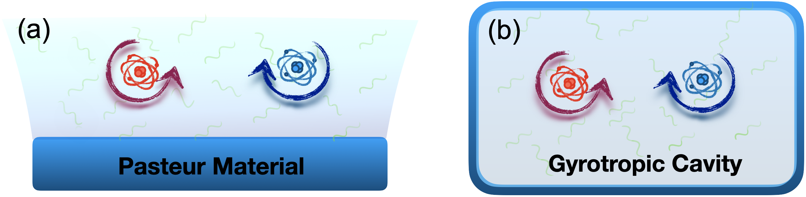
Figure 1: A pair of enantiomers (red and blue colors refer to opposite chirality) immersed in PS-broken quantum fluctuations proximate to a Pasteur material (a) and in a gyrotropic cavity (b).

The paper is organized as follows: We first review the theoretical model of chiral molecules based on the Born-Oppenheimer (BO) approximationBorn and Oppenheimer (1927). Second, we identify a chiral energy shift that can characterize chiral ensembles in a PS-broken vacuum. Through first-principle calculation, we uncover a sizable energy disparity of a pair of enantiomers. Finally, we evaluate the chemical reaction rate and obtain a notable chirality production rate, amply illustrating the selective power of symmetry-broken quantum fluctuations.

BO approximation and the model of chiral molecules.— The Hamiltonian of a molecule contains three parts: the energy of nucleus, the energy of electrons, and the interaction energy between the electrons and the nucleus:

$$\widehat{H}_{mol}=\widehat{T}_{n}+\widehat{V}_{n}(\hat{\mathbb{R}})+\widehat{T}_{el}+\widehat{V}_{el}(\hat{\mathbb{r}})+\widehat{V}_{n-el}(\hat{\mathbb{R}},\hat{\mathbb{r}}).$$ (1)

Here, $\widehat{T}$ and $\widehat{V}$ denote the kinetic energy and Coulomb interactions, respectively; subindices $n$ and $el$ represent nucleus and electrons, respectively; variables $\left\{\mathbb{R}_{1},\mathbb{R}_{2},\dots,\mathbb{R}_{N_{1}}\right\}$ and $\left\{\mathbb{r}_{1},\mathbb{r}_{2},\dots,\mathbb{r}_{N_{2}}\right\}$ stand for the positions of $N_{1}$ nucleus and $N_{2}$ electrons, respectively.

BO approximation is based on the fact that the kinetic energy of electrons is much larger than the nucleus. The energy-scale separation allows one to treat the electron movement first while the nuclear positions are regarded as fixed parameters. According to this scenario, the BO approximation is a two-step procedureBorn and Oppenheimer (1927); Henriksen and Hansen (2018):

1. Solve the electronic Hamiltonian $\widehat{H}_{el}=\widehat{T}_{el}+\widehat{V}_{el}+\widehat{V}_{n-el}(\mathbb{R},\hat{\mathbb{r}}),$ whose $i$-th eigenenergy and eigenstate are functions of $\mathbb{R}$, denoted as $E_{el,i}(\mathbb{R})$ and $|\phi_{i}(\mathbb{R})\rangle$ $(i=0,1,2...)$, respectively.

2. Promoting $\mathbf{R}$ to be an operator yields an $\mathbf{\hat{R}}$-dependent electronic Hamiltonian $\widehat{H}_{el}(\mathbf{\hat{R}})=\sum_{i}E_{el,i}(\mathbf{\hat{R}})|\phi_{i}(\mathbf{\hat{R}})\rangle\langle\phi_{i}(\mathbf{\hat{R}})|$.

The potential energy surface (PES) for the $i$th electronic energy level is defined as

$${{\widehat{V}}_{i}}({{\mathbf{\hat{R}}}})\equiv{{\widehat{V}}_{n}}({{\mathbf{\hat{R}}}})+E_{el,i}(\mathbf{\hat{R}})|\phi_{i}(\mathbf{\hat{R}})\rangle\langle\phi_{i}(\mathbf{\hat{R}})|.$$ (2)

Because of the well-separated PESs, the transition between different PESs can be ignored, and the effective Hamiltonian for the $i$th PES reduces to ${{\widehat{H}}^{(i)}_{mol}}={{\widehat{T}}_{n}}({{\mathbf{\hat{R}}}})+{{\widehat{V}}_{i}}({{\mathbf{\hat{R}}}})$. We will focus on the shift of the ground-state PES of a chiral molecule induced by PS-broken quantum fluctuations.

To characterize chiral molecules, we introduce a parity operator $\mathcal{J}_{P}$ and a rotation operator $\mathcal{J}_{R}$. For a chiral molecule, any rotation of nuclear configurations could not bring the electronic Hamiltonian identical to its enantiomer, i.e., ${{\widehat{H}}_{el}}(\mathcal{J}_{R}\mathbf{\hat{R}})\neq{{\widehat{H}}_{el}}(\mathcal{J}_{P}\mathbf{\hat{R}})$ for all $\mathcal{J}_{R}\in{\rm SO(3)}$. By contrast, for achiral molecules, there always exists a rotation operation that can bring the electronic Hamiltonian identical to its parity counterpart.

Energy shift of chiral molecules in vacuum.— We consider a molecule interacting with a nearby symmetry-broken material through vacuum quantum EM fluctuations. Within the BO approximation, and the total Hamiltonian consists the electronic Hamiltonian $\widehat{H}_{el}$ of the molecule, the vacuum EM Hamiltonian $\widehat{H}_{em}$, the electron-EM interaction $\widehat{H}_{el-em}$, and the material-EM interaction $\widehat{H}_{mat-em}$:

$$\widehat{H}=\widehat{H}_{el}+\widehat{H}_{el-em}+\widehat{H}_{em}+\widehat{H}_{mat-em}.$$ (3)

Tracing out the material degrees of freedom $|\psi_{mat}\rangle$ yields an effective Hamiltonian $H_{sb}$ that embodies the symmetry-breaking information of the material:

$$\widehat{H}_{sb}=\widehat{H}_{em}+{\rm Tr}_{mat}\left(\widehat{H}_{mat-em}\right)$$ (4)

where ${\rm Tr}_{mat}$ denotes the trace of the matrix with respect to the states of the material. Since $\widehat{H}_{sb}$ encodes all the material’s influence on the vacuum EM fields, a simplified Hamiltonian can be employed to address the interaction between the molecules and the symmetry-broken material:

$$\widehat{H}=\widehat{H}_{el}+\widehat{H}_{el-em}+\widehat{H}_{sb}.$$ (5)

When considering the interactions between molecules and EM fields, the important Fourier components of EM fields are those whose frequencies are on the order of atomic frequencies or less. Since the corresponding wavelength is much larger than the size of the molecule, one could employ the interaction Hamiltonian in the multipolar coupling scheme and long-wavelength approximation, describing the interaction of a molecule with the EM fields: $\widehat{H}_{el-em}=-\mathbf{\widehat{d}}\cdot\mathbf{\widehat{E}}-\mathbf{\widehat{m}}\cdot\mathbf{\widehat{B}}$, where $\mathbb{d}$ and $\mathbb{m}$ denote the electric and magnetic dipoles of the molecule, respectively. This multipolar coupling Hamiltonian has been extensively studied in the literaturePower and Thirunamachandran (1983); Salam and Thirunamachandran (1994); Salam (1997); Jenkins et al. (1994); Butcher et al. (2012). Electromagnetic quantum fluctuations renormalize the electronic energy levels, yielding a shift of the ground-state energy (we use the unit $\hbar=c=1$)

$$\Delta E_{0}=-\sum_{i,I,F}p(I)\frac{\left|\left\langle\phi_{i},F\left|\widehat{\mathbb{d}}\cdot\widehat{\mathbb{E}}+\widehat{\mathbb{m}}\cdot\widehat{\mathbb{B}}\right|\phi_{0},I\right\rangle\right|^{2}}{E_{i0}+\Omega_{FI}}.$$

Here, $|\phi_{i},I\rangle\equiv|\phi_{i}(\mathbb{R})\rangle\otimes|I\rangle$ is the direct product state of the $i$th PES’s state $|\phi_{i}(\mathbb{R})\rangle$ and the photonic state $|I\rangle$. $p(I)=e^{-\beta E_{I}}/Z_{ph}$ is the thermal probability of the initial photonic state $|I\rangle$. $E_{i0}$ is the energy gap between the $i$th PES and the lowest PES. $\Omega_{FI}=\Omega_{F}-\Omega_{I}$ is the energy gap between the photonic states $|F\rangle$ and $|I\rangle$.

The ground-state energy shift includes two parts: The first contribution

$$\Delta E_{0}^{a\chi}=-\sum\limits_{i,I,F}p(I)\frac{\left|\mathbf{d}_{0i}\cdot\mathbf{E}_{IF}\right|^{2}+\left|\mathbf{m}_{0i}\cdot\mathbf{B}_{IF}\right|^{2}}{E_{i0}+\Omega_{FI}}$$ (6)

is achiral, because it remains invariant under a parity operation (i.e., $\mathbb{m}\rightarrow\mathbb{m}$ and $\mathbb{d}\rightarrow-\mathbb{d}$). By contrast, the second contribution

$$\Delta E_{0}^{\chi}=-\sum_{i,I,F}p(I)\frac{2\,{\rm Re}\left[\left(\mathbb{d}_{0i}\cdot\mathbb{E}_{IF}\right)\left(\mathbb{m}_{i0}\cdot\mathbb{B}_{FI}\right)\right]}{E_{i0}+\Omega_{FI}}$$ (7)

reverses its sign under the parity operation and is called chiral energy shift. The transition matrices are defined as $\mathbb{d}_{0i}=\langle\phi_{0}|\widehat{\mathbb{d}}|\phi_{i}\rangle$, $\mathbb{m}_{i0}=\langle\phi_{i}|\widehat{\mathbb{m}}|\phi_{0}\rangle$, $\mathbb{E}_{IF}=\langle I|\mathbb{\widehat{E}}|F\rangle$, and $\mathbb{B}_{FI}=\langle F|\mathbb{\widehat{B}}|I\rangle$.

The chiral energy shift arises for a molecule (regardless of being chiral or not) with finite electronic and magnetic dipoles. However, to calculate the average chiral energy shift of an isotropic ensemble (liquid or gas), one should integrate over all orientations. And that makes the key difference: The average chiral energy shift vanishes for achiral ensembles but remains finite for chiral ensembles (see the proof ):

$$\langle\Delta E_{0}^{\chi}\rangle=-\sum_{i,I,F}\frac{2\,p(I)\,{\rm Re}\left[\mathcal{R}_{i0}\left(\mathbb{E}_{IF}\cdot\mathbb{B}_{FI}\right)\right]}{3\left(E_{i0}+\Omega_{FI}\right)},$$ (8)

where $\mathcal{R}_{i0}\equiv\left(\mathbb{d}_{0i}\cdot\mathbb{m}_{i0}\right)$, the imaginary part of which is called rotatory strengthCraig and Thirunamachandran (1998); Barron (2009). In what follows, we will evaluate the chiral energy shift of chiral molecules induced by two types of PS-broken quantum fluctuations.

Chiral molecules above a Pasteur material.— The EM response of a Pasteur material is governed by the constitutive relations $\mathbb{D}=\epsilon\mathbb{E}-i\kappa\mathbb{H}$ and $\mathbb{B}=\mu\mathbb{H}+i\kappa\mathbb{E}$, where, following Landau’s convention, $\mathbb{D}$ and $\mathbb{B}$ ($\mathbb{E}$ and $\mathbb{H}$) are called electric and magnetic induction (field); $\epsilon=\epsilon_{r}\epsilon_{0}$ ($\mu=\mu_{r}\mu_{0}$) are the permittivity (permeability) of the Pasteur materialLindell et al. (1994); the parameter $\kappa$ characterizes the strength of PS breaking. While the Casimir-Polder forces between a chiral molecule and a Pasteur material have been nicely investigatedButcher et al. (2012), we focus on the spectral change.

We can alternatively express Eq. (8) in terms of Green’s functions:

$$\langle\Delta E_{0}^{\chi}\rangle=\frac{{2{\mu_{0}}}}{{3\pi}}\sum\limits_{i}{\text{Im}}{\mathcal{R}_{i0}}{\int_{0}^{+\infty}{\frac{{{\xi^{2}}d\xi}}{{E_{i0}^{2}+{\xi^{2}}}}{\text{Tr}}\nabla\times{\mathbf{G}}\left({i\xi}\right)}}$$ (9)

with $\mathbb{G}$ the Green’s function of EM fields, which includes the free-space contribution $\mathbb{G}_{free}$ and the symmetry-breaking contribution from Pasteur material $\mathbb{G}_{sb}$. Similar formulas Eqs.(6), (7), and (9) have been used to derive chiral-surface-molecule interactions and chiral-surface-mediated interactions previouslyButcher et al. (2012); Barcellona et al. (2017). While the free-space contribution embodies no symmetry-breaking information and leads to identical energy shift for enantiomers, the symmetry-breaking contribution differentiates chiral enantiomers. One can obtain $\mathbb{G}_{sb}$ from the reflection coefficients of the Pasteur plate, namely $r_{ss}$, $r_{sp}$, $r_{ps}$, and $r_{pp}$, where the subindices indicate the polarization of the incoming and reflected EM wave. We numerically calculate the distance-dependent energy shift, and compare it with the analytical nonretarded limit $\frac{{{\mu_{0}}\left({{r_{sp}}-{r_{ps}}}\right)}}{{48i\pi{z^{3}}}}\operatorname{Im}{\mathcal{R}_{eg}}$ (Fig. 2). Here, $z$ is the distance between the chiral molecule and Pasteur plate, and ${\rm Im}\mathcal{R}_{10}$ is the rotatory strength considering the molecular ground state and its first excited state.

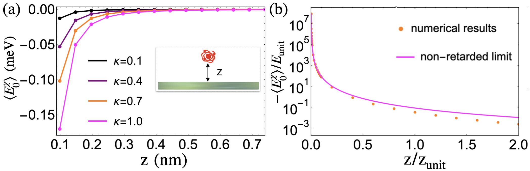
Figure 2: (a) Numerically calculation of average chiral energy shift for different parameter $\kappa$. We set $E_{10}=2\,{\rm eV}$ and $\operatorname{Im}\mathcal{R}_{10}=0.1ea_{0}\mu_{B}$ with $a_{0}$ and $\mu_{B}$ the Bohr radius and Bohr magnetic moment, respectively. (b) The analytical nonretarded result works for $z\ll z_{\rm unit}=1/E_{10}$; the energy unit is defined as $E_{\rm unit}={\mu_{0}\operatorname{Im}\mathcal{R}_{10}E_{10}^{3}}/{3\pi^{2}}$; $\kappa=0.4$. We set ${\varepsilon_{r}}={\mu_{r}}=1$.

Chiral molecules in gyrotropic cavities.— We study chiral molecules in a PS-broken gyrotropic cavity. The Hamiltonian for the cavity photonic modes reads $\hat{H}_{qa}=\sum_{n}\Omega_{n}\left(\hat{a}_{n}^{\dagger}\hat{a}_{n}+\frac{1}{2}\right)$, where $\hat{a}_{n}^{\dagger}$ is the creation operator of a photonic mode $n$ and frequency $\Omega_{n}$. In terms of creation and annihilation operators, the vector potential is

$$\mathbb{\hat{A}}(\mathbb{r})=\sum_{n}g_{n}\left[\mathbb{A}_{n}(\mathbb{r})\hat{a}_{n}+\mathbb{A}_{n}^{*}(\mathbb{r})\hat{a}_{n}^{\dagger}\right],$$ (10)

where the coupling strength $g_{n}=\sqrt{{1}/{2\epsilon_{0}\Omega_{n}V_{{\rm eff}}}}$; and $\mathbb{A}_{n}(\mathbb{r})=e^{i\mathbb{k}_{n}\cdot\mathbb{r}}\mathbf{\hat{e}}$ represents the EM wave of polarization $\mathbf{\hat{e}}$. We assume a general polarization $\mathbf{\hat{e}}=\mathbb{\hat{e}}_{R}+i\mathbb{\hat{e}}_{I}$ with real $\mathbf{\hat{e}}_{R}$ and $\mathbf{\hat{e}}_{I}$, which encodes the symmetry-broken information. Substituting the EM fields operators (Coulomb gauge)

$$\hat{\mathbb{E}}(\mathbb{r}) =i\sum_{n}g_{n}\Omega_{n}\left[\mathbb{A}_{n}(\mathbb{r})\hat{a}-\mathbb{A}_{n}^{*}(\mathbb{r})\hat{a}^{\dagger}\right],~{}\text{and}$$ (11)

$$\hat{\mathbb{B}}(\mathbb{r}) =i\sum_{n}g_{n}\left[\boldsymbol{\nabla}\times\mathbb{A}_{n}(\mathbb{r})\hat{a}+\boldsymbol{\nabla}\times\mathbb{A}_{n}^{*}(\mathbb{r})\hat{a}^{\dagger}\right]$$

into Eq. (8) yields the chiral energy shift

$$\langle\Delta E_{0}^{\chi}\rangle=\sum_{n}\frac{4g_{n}^{2}\Omega_{n}^{2}}{3}\mathbb{\hat{e}_{k}}\cdot\left(\mathbb{\hat{e}}_{R}\times\mathbb{\hat{e}}_{I}\right)\sum_{i}\frac{{\rm Im}\mathcal{R}_{i0}}{E_{i0}+\Omega_{n}}.$$ (12)

Here, the factor $\mathbb{\hat{e}_{k}}\cdot\left(\mathbb{\hat{e}}_{R}\times\mathbb{\hat{e}}_{I}\right)$ flips sign under parity operation and implies the chirality of the cavity mode. $\mathbb{\hat{e}_{k}}\cdot\left(\mathbb{\hat{e}}_{R}\times\mathbb{\hat{e}}_{I}\right)=\pm\frac{1}{2}$ for a right(left)-handed circularly polarized mode, whereas it vanishes in a linearly polarized one. Let us estimate the magnitude of the chiral energy shift with promising experimental parameters. Considering two-level systems (ground state $|g\rangle$ and excited state $|e\rangle$), we estimate the chiral energy shift in a left-handed gyrotropic cavity

$$\langle\Delta E_{0}^{\chi}\rangle=-\frac{4\pi\alpha}{3}\sum_{n}\left(\frac{{\rm Im}\mathcal{R}_{eg}}{ea_{0}\mu_{B}}\right)\left(\frac{a_{0}^{3}}{V_{\rm eff}}\right)\frac{\Omega_{n}}{{\Delta E+\Omega_{n}}}E_{\rm Ryd}$$ (13)

where $\alpha$, $a_{0}$, and $\mu_{B}$ are the fine structure constant, Bohr radius, and Bohr magnetic moment, respectively. $\Delta E$ denotes the electronic energy gap; $\Omega_{n}$ is the frequency of the $n$th photonic mode; $E_{\rm Ryd}$ is the Rydberg energy; ${\rm Im}\mathcal{R}_{eg}$ is the molecular rotatory strength, and the effective mode volume of a cavity is defined as the ratio between the total field energy in the cavity divided by the field energy density at the molecular position, i.e., ${V_{\rm eff}}=\int_{V}{{d^{3}}r\varepsilon\left({\mathbf{r}}\right){{\left|{{\mathbf{E}}\left({\mathbf{r}}\right)}\right|}^{2}}}/{\epsilon_{0}\left|{{\mathbf{E}}\left({{{\mathbf{r}}_{m}}}\right)}\right|^{2}}$. Setting ${\rm Im}\mathcal{R}_{eg}\approx 0.1\,ea_{0}\mu_{B}$, $\Delta E\approx 2\,{\rm eV}$, $\Omega_{n}=0.1n\,{\rm eV}$ (ten modes $n=1,2...10$), and the smallest effective volume reachable in experiments $V_{\rm eff}\approx 0.2\,\text{nm}^{3}$, we obtain an experimental detectable chiral energy shift $\overline{\delta E_{0}^{\rm\chi}}\approx-0.06\,{\rm meV}$.

Figure 3: (a) Atomic structure of a chiral molecule and its enantiomer. Gray and white balls represent carbon and hydrogen atoms, respectively. (b) DFT calculated electric dipole as a function of the reaction coordinate. The reaction coordinate is defined as a certain average of nuclei displacement, which captures the change of molecular configuration. The reaction coordinate is defined as a certain average displacement of nucleus, capturing the change of molecular configuration. (c) Bare molecular PES. The barrier is symmetric for left-handed and right-handed molecules. (d) Molecular PES versus the reaction coordinate induced by chiral energy shift [see Eq. (16)]. Different colors correspond to different numbers of molecules.

Collective enhancement.— Here, we explore how the chiral energy shift can be enhanced by collective effects. For this analysis, it is important to identify two types of terms in Eq. (7), commonly called the Debye term ($i=0$) and the London term ($i\neq 0$). While both terms contribute to the measurable spectral shift, only the Debye term can benefit from collective effect in a polarized ensemble of molecules (see below). Similar to Eq. (7), we calculate the Debye part of the chiral energy shift of all $N$ molecules at zero temperature:

$${\left.{\Delta E_{0,N}^{\chi}}\right|_{{\text{Debye}}}}\hfill$$

$$=-\sum\limits_{n}{\frac{{2\operatorname{Re}\left[{\left({\sum\limits_{j=1}^{N}{{\mathbf{d}}_{00}^{\left(j\right)}\cdot{{\mathbf{E}}_{n,01}^{(j)}}}}\right)\left({\sum\limits_{j=1}^{N}{{\mathbf{m}}_{00}^{\left(j\right)}\cdot{{\mathbf{B}}_{n,10}^{(j)}}}}\right)}\right]}}{{{\Omega_{n}}}}}$$

$$=-{N^{2}}\sum\limits_{n}{\frac{{2\operatorname{Re}\left[{\left({{\mathbf{d}}_{00}\cdot{{\mathbf{E}}_{n,01}}}\right)\left({{\mathbf{m}}_{00}\cdot{{\mathbf{B}}_{n,10}}}\right)}\right]}}{{{\Omega_{n}}}}}$$ (14)

where $n$ labels the cavity modes, and $(j)$ represents the physical quantities of the $j$th molecule. The second equality follows that the molecules are polarized, ${\mathbf{d}}_{00}^{\left(j\right)}\cdot{{\mathbf{E}}_{n,01}^{(j)}}={\mathbf{d}}_{00}\cdot{{\mathbf{E}}_{n,01}},\,{\mathbf{m}}_{00}^{\left(j\right)}\cdot{{\mathbf{B}}_{n,10}^{(j)}}={\mathbf{m}}_{00}\cdot{{\mathbf{B}}_{n,10}}$. (A similar derivation was also given in Galego et al. (2019).) Modeling chiral cavity modes the same as before, the Debye term per molecule is

$${\left.{\Delta E_{0}^{\chi}}\right|_{{\text{Debye}}}}= -N\sum\limits_{n}{\frac{{2\operatorname{Re}\left[{\left({{{\mathbf{d}}_{00}}\cdot{{\mathbf{E}}_{n,01}}}\right)\left({{{\mathbf{m}}_{00}}\cdot{{\mathbf{B}}_{n,10}}}\right)}\right]}}{{{\Omega_{n}}}}}\hfill$$ (15)

$$= -N\sum\limits_{n}{g_{n}^{2}\Omega_{n}\left({{d_{00,x}}{m_{00,y}}-{d_{00,y}}{m_{00,x}}}\right)}\hfill$$

To illustrate the opposite energy shift for a pair of enantiomers, we consider a concrete example — an ensemble of chiral molecules named hydrogen-missing helicene [Fig. 3(a)]. Using density functional theory (DFT), we calculate the ground-state electric dipole moment of this molecule as it undergoes a transition from left-handed to right-handed configuration [Fig. 3(b)]. Enantiomers are mirror images of each other across the $y$-$z$ plane, resulting in dipole moments of $\left({\pm{d_{00,x}},{d_{00,y}},{d_{00,z}}}\right)$. The ground-state magnetic moment arises from an unpaired electron, which can be polarized in the $y$ direction. Consequently, the pair of enantiomers experience opposite chiral energy shifts (note that the London term does not scale with $N$ and can be ignored here ):

$$\Delta E_{0}^{\chi}\approx{\left.{\Delta E_{0}^{\chi}}\right|_{{\text{Debye}}}}=\mp N\sum\limits_{n}{g_{n}^{2}\Omega_{n}{d_{00,x}}{m_{00,y}}}$$ (16)

Using the same parameters as given below Eq. (13) except with ${{\mathbf{d}}_{00}}=0.2e{a_{0}}{{\mathbf{e}}_{x}}$ and ${{\mathbf{m}}_{00}}={\mu_{B}}{{\mathbf{e}}_{y}}$, we find the magnitude $\mp N\times 0.92\,{\text{meV}}$. Our DFT calculations in Fig. 3(d) show that the chiral energy shift in a cluster of 100 molecules can be significantly enhanced. We have not considered the effect of intermolecular interactionsJenkins et al. (1994); Salam and Thirunamachandran (1994); Safari et al. (2020), which may influence the collective enhancement quantitatively by either strengthening or weakening the molecular alignment.

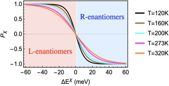
Figure 4: Chirality-selective rate as a function of the chiral energy shift at different temperatures. Upon reversing the chiral energy shift, opposite chirality is selected.

Finally, we evaluate the impact of chiral energy shift in chemical reactions. According to the collision theory, chemical reaction rates depends on the activation energy $E_{a}$—a minimum amount of energy that the reactants need to overcome to form products. The chemical reaction rates can be approximately calculated by the Arrhenius equation $k=A\exp(-\beta E_{a})$ ($k$ is the rate constant and $E_{a}$ is the activation energy)Laidler (1984). We define a chirality-selective rate to characterize the reaction-rate difference between chiral enantiomers:

$$P_{\chi}=\frac{k_{L}-k_{R}}{k_{L}+k_{R}}=\frac{1-\exp{\left(-2\beta{\Delta E_{0}^{\chi}}\right)}}{1+\exp{\left(-2\beta{\Delta E_{0}^{\chi}}\right)}}$$ (17)

with $k_{L}$ ($k_{R}$) denoting the chemical reaction rates for the L(D) enantiomer. In Supplemental Material , we use transition state theory to justify the above result. One could tune the sign of the chiral energy shift to select desired chirality in chemical reactions (see Fig. 4).

Summary.— We studied the effect of quantum fluctuations on the spectra of chiral molecules. Our research demonstrates that PS-broken quantum fluctuations can induce a chirality-dependent shift in the ground-state energy. We predicted a significant rate of chirality selection for chiral enantiomers in a gyrotropic cavity. Since chirality selection is related to the rotational strength or the ground-state dipole moments (generally nonzero), our findings have broad applicability and are not limited to any specific molecular model. We remark that our logic, content, and proposals differ fundamentally from the recent papers discussing chirality discriminationRiso et al. (2023); Vu et al. (2022).

The authors gratefully acknowledge helpful discussions and suggestions from anonymous referees. We are sponsored by Pujiang Talent Program 21PJ1405400, TDLI starting up grant, Jiaoda 2030 program WH510363001, and Innovation Program for Quantum Science and Technology Grant No.2021ZD0301900.

Supplemental Materials

The supplemental materials are structured as follows:

• Section A discusses the average of chiral energy shift across all spatial orientations, as given by Equation (8).

• Sections B and C are dedicated to the scattering Green’s function method for calculating the chiral energy shift. The specific calculation for the Pasteur plate case can be found in Section C.

• Section D presents the derivation of the chiral energy shift in a gyrotropic cavity, as given by Equation (12).

• Section E explores the effects of finite temperature on our results.

• Section F provides an explanation of the approximations utilized in the Arrhenius equation we employ.

• Section G contains information regarding the density functional theory calculation.

Appendix A Isotropic average of chiral energy shift

In this section, we delve deeper into the derivation of averaging the chiral energy shift over various molecular orientations. We provide the derivation of Equation (8) presented in the main text and explain the reason behind its vanishing value for achiral molecules. Considering a molecule with nuclear positions denoted as $\mathbf{R}$, the chiral energy shift can be expressed as:

$${\Delta E_{0}^{\chi}}=-\sum\limits_{i,I,F}{{p_{I}}\frac{{2\operatorname{Re}\left({{{\mathbf{d}}_{0i}}\left({\mathbf{R}}\right)\cdot{{\mathbf{E}}_{IF}}}\right)\left({{{\mathbf{m}}_{i0}}\left({\mathbf{R}}\right)\cdot{{\mathbf{B}}_{FI}}}\right)}}{{{E_{i0}}+{\omega_{FI}}}}}$$ (18)

It is important to note that the matrix elements of electric and magnetic dipoles are dependent on the orientation of $\mathbf{R}$. In the case of isotropic samples of molecules, as discussed in the main text, it is necessary to take an average over all orientations. Therefore, the expression can be written as follows:

$$\left\langle{\Delta E_{0}^{\chi}}\right\rangle=-\int_{{\mathcal{J}_{R}}\in{\text{SO}}\left(3\right)}{d{\mathcal{J}_{R}}\sum\limits_{i,I,F}{{p_{I}}\frac{{2\operatorname{Re}\left({{{\mathbf{d}}_{0i}}\left({{\mathcal{J}_{R}}{\mathbf{R}}}\right)\cdot{{\mathbf{E}}_{IF}}}\right)\left({{{\mathbf{m}}_{i0}}\left({{\mathcal{J}_{R}}{\mathbf{R}}}\right)\cdot{{\mathbf{B}}_{FI}}}\right)}}{{{E_{i0}}+{\omega_{FI}}}}}}$$ (19)

But what are ${{\mathbf{d}}_{0i}}\left({{\mathcal{J}_{R}}{\mathbf{R}}}\right)$ and ${{\mathbf{m}}_{0i}}\left({{\mathcal{J}_{R}}{\mathbf{R}}}\right)$? Define a unitary representation of SO(3), $\hat{J}_{R}$, acting on electronic position eigenstates as ${\hat{J}_{R}}\left|{\mathbf{r}}\right\rangle=\left|{{\mathcal{J}_{R}}{\mathbf{r}}}\right\rangle$. Then, using the fact that electronic Hamiltonian (see the discussion of BO approximation in the main text) is unchanged under rotating both the nuclear and electronic positions, $\hat{J}_{R}^{-1}H\left({{\mathcal{J}_{R}}{\mathbf{R}}}\right){{\hat{J}}_{R}}=H\left({\mathbf{R}}\right)$, one can verify that $\left|{{\phi_{i}}\left({{\mathcal{J}_{R}}{\mathbf{R}}}\right)}\right\rangle={{\hat{J}}_{R}}\left|{{\phi_{i}}\left({\mathbf{R}}\right)}\right\rangle$. Moreover, for matrix elements of electric dipole moment,

$${{\mathbf{d}}_{ij}}\left({\mathbf{R}}\right)= \sum\nolimits_{\alpha\in\{{\text{nuclei}}\}}{{Z_{\alpha}}e{{\mathbf{R}}_{\alpha}}}-\left\langle{{\phi_{i}}\left({\mathbf{R}}\right)}\right|\sum\nolimits_{\beta\in\{{\text{electrons}}\}}{e{{\hat{\mathbf{r}}}_{\beta}}}\left|{{\phi_{j}}\left({\mathbf{R}}\right)}\right\rangle\hfill$$ (20)

$${{\mathbf{d}}_{ij}}\left({{\mathcal{J}_{R}}{\mathbf{R}}}\right)= \sum\nolimits_{\alpha\in\{{\text{nuclei}}\}}{{Z_{\alpha}}e{\mathcal{J}_{R}}{{\mathbf{R}}_{\alpha}}}-\left\langle{{\phi_{i}}\left({\mathbf{R}}\right)}\right|\hat{J}_{R}^{-1}\sum\nolimits_{\beta\in\{{\text{electrons}}\}}{e{{\hat{\mathbf{r}}}_{\beta}}}{{\hat{J}}_{R}}\left|{{\phi_{j}}\left({\mathbf{R}}\right)}\right\rangle\hfill$$

$$= {\mathcal{J}_{R}}{{\mathbf{d}}_{ij}}\left({\mathbf{R}}\right)\hfill$$

Similarly, magnetic moment $\displaystyle{{\mathbf{m}}_{ij}}\left({\mathbf{R}}\right)=\left\langle{{\phi_{i}}\left({\mathbf{R}}\right)}\right|\sum\nolimits_{\beta\in\{{\text{electrons}}\}}{\frac{{-e}}{{2{m_{e}}}}{{{\mathbf{\hat{r}}}}_{\beta}}\times{{{\mathbf{\hat{p}}}}_{\beta}}}\left|{{\phi_{j}}\left({\mathbf{R}}\right)}\right\rangle$ satisfies

$${{\mathbf{m}}_{ij}}\left({{\mathcal{J}_{R}}{\mathbf{R}}}\right)={\mathcal{J}_{R}}{{\mathbf{m}}_{ij}}\left({\mathbf{R}}\right)$$ (21)

Also, for parity operator introduced in the main text, ${\mathcal{J}_{P}}$, which is a spatial inversion around the center of a molecule, one can prove that

$${{\mathbf{d}}_{ij}}\left({{\mathcal{J}_{P}}{\mathbf{R}}}\right)=-{{\mathbf{d}}_{ij}}\left({\mathbf{R}}\right),{{\mathbf{m}}_{ij}}\left({{\mathcal{J}_{P}}{\mathbf{R}}}\right)={{\mathbf{m}}_{ij}}\left({\mathbf{R}}\right)$$ (22)

Using these definitions, (19) becomes

$$\left\langle{\Delta E_{0}^{\chi}}\right\rangle= -\int_{{\mathcal{J}_{R}}\in{\text{SO}}\left(3\right)}{d{\mathcal{J}_{R}}\sum\limits_{i,I,F}{{p_{I}}\frac{{2\operatorname{Re}\left[{\left({{\mathcal{J}_{R}}{{\mathbf{d}}_{0i}}\cdot{{\mathbf{E}}_{IF}}}\right)\left({{\mathcal{J}_{R}}{{\mathbf{m}}_{i0}}\cdot{{\mathbf{B}}_{FI}}}\right)}\right]}}{{{E_{i0}}+{\omega_{FI}}}}}}\hfill$$ (23)

$$= -\frac{2}{3}\sum\limits_{i,I,F}{{p_{I}}\frac{{\operatorname{Re}\left[{\left({{{\mathbf{d}}_{0i}}\cdot{{\mathbf{m}}_{i0}}}\right)\left({{{\mathbf{E}}_{IF}}\cdot{{\mathbf{B}}_{FI}}}\right)}\right]}}{{{E_{i0}}+{\omega_{FI}}}}}\hfill$$

This is eq.8 in the main text. Note that ${{{\mathbf{d}}_{0i}}\cdot{{\mathbf{m}}_{i0}}}$ changes sign under parity operation, $\left\langle{\Delta E_{0}^{\chi}\left({{\mathcal{J}_{P}}{\mathbf{R}}}\right)}\right\rangle=-\left\langle{\Delta E_{0}^{\chi}\left({\mathbf{R}}\right)}\right\rangle$. However, as mentioned in the main text, for an achiral molecule, there is a specific rotation $\mathcal{J}_{{R_{0}}}$, s.t. $H\left({{\mathcal{J}_{{R_{0}}}}{\mathbf{R}}}\right)=H\left({{\mathcal{J}_{P}}{\mathbf{R}}}\right)$ and $\left\langle{\Delta E_{0}^{\chi}\left({{\mathcal{J}_{{R_{0}}}}{\mathbf{R}}}\right)}\right\rangle=\left\langle{\Delta E_{0}^{\chi}\left({{\mathcal{J}_{P}}{\mathbf{R}}}\right)}\right\rangle$. So,

$$\left\langle{\Delta E_{0}^{\chi}\left({{\mathcal{J}_{P}}{\mathbf{R}}}\right)}\right\rangle= \int_{{J_{R}}\in{\text{SO}}\left(3\right)}{d{\mathcal{J}_{R}}\delta E_{0}^{{\text{ch}}}\left({{\mathcal{J}_{R}}{\mathcal{J}_{P}}{\mathbf{R}}}\right)}\hfill$$

$$= \int_{{J_{R}}\in{\text{SO}}\left(3\right)}{d{\mathcal{J}_{R}}\delta E_{0}^{{\text{ch}}}\left({{\mathcal{J}_{{R_{0}}}}{\mathcal{J}_{R}}{\mathbf{R}}}\right)}\hfill$$

$$= \left\langle{\Delta E_{0}^{\chi}\left({\mathbf{R}}\right)}\right\rangle\hfill$$

In the second equality we use that parity and rotation commute. Therefore, average chiral energy shift indeed vanishes for achiral molecules.

Appendix B Chiral Casimir-Polder energy in electromagnetic Green’s function

In this section, we derive the explicit expression for chiral Casimir-Polder energy using electromagnetic Green’s function, i.e., Eq.(9) in the main text, on which the next section is based.

According to Eq.(7) of the main text, the chiral energy shift is,

$$\Delta E_{0}^{\chi}\left({{{\mathbf{r}}_{M}}}\right)=-\sum\limits_{i,I,F}{p\left(I\right)\frac{{2\operatorname{Re}\left[{{{\mathbf{d}}_{0i}}\cdot{{\mathbf{E}}_{IF}}\left({{{\mathbf{r}}_{M}}}\right)\otimes{{\mathbf{B}}_{IF}}\left({{{\mathbf{r}}_{M}}}\right)\cdot{{\mathbf{m}}_{i0}}}\right]}}{{{E_{i0}}+{E_{FI}}}}}$$ (24)

where we combine vectors $\mathbf{E}$ and $\mathbf{B}$ to be a tensor.

Electromagnetic Green’s function is a useful tool for studying this problem. Roughly, it is both the Green’s function for the equation of motion of vector potential in $\phi=0$ gauge, obeying $\left({-\frac{{{\omega^{2}}}}{{{c^{2}}}}{\varepsilon_{r}}\left({{\mathbf{r}},\omega}\right)+\nabla\times\frac{1}{{{\mu_{r}}\left({{\mathbf{r}},\omega}\right)}}\nabla\times}\right){\mathbf{G}}\left({{\mathbf{r}},{\mathbf{r}}^{\prime},\omega}\right)=\delta\left({{\mathbf{r}}-{\mathbf{r}}^{\prime}}\right)$ (where Pasteur parameter $\kappa$ is zero for simplicity), and the retarded response function of vector potential (times $-\mu_{0}^{-1}$) (For an introduction to electromagnetic Green’s function, see Ref.[S1,S2]). To use Green’s function in the following derivation, we need the analytic structure of correlation function. The frequency domain retarded response function of operators ${\widehat{O}_{1,2}}$ is ${G^{R}_{12}}\left(\omega\right)={Z^{-1}}\sum\limits_{I,F}{{O_{1,IF}}{O_{2,FI}}\frac{{{e^{-\beta{E_{I}}}}-{e^{-\beta{E_{F}}}}}}{{\omega+{E_{IF}}+i0+}}}$. Generalized imaginary part can be defined as $\operatorname{Im}^{\prime}{G^{R}}(\omega)=\frac{1}{2i}\left[{G_{12}^{R}(\omega)-G_{21}^{R\;*}(\omega)}\right]$, and thus

$$\operatorname{Im}^{\prime}{G^{R}}\left(\omega\right)=-\pi\sum\limits_{I,F}{p\left(I\right){O_{1,IF}}{O_{2,FI}}\left({1-{e^{-\beta\omega}}}\right)\delta\left({\omega-{E_{FI}}}\right)}$$ (25)

Therefore, we have the following expression of the generalized imaginary part of the correlation function of electric and magnetic fields

$$-\frac{1}{\pi}\int_{-\infty}^{+\infty}{d\omega\frac{{\operatorname{Im}^{\prime}{\mathbf{G}}_{em}^{R}\left({{\mathbf{r}},{\mathbf{r}}^{\prime},\omega}\right)}}{{\left({1-{e^{-\beta\omega}}}\right)\left({{E_{i0}}+\omega}\right)}}}=\sum\limits_{I,F}{p\left(I\right)\frac{{{{\mathbf{E}}_{IF}}\left({\mathbf{r}}\right)\otimes{{\mathbf{B}}_{IF}}\left({{\mathbf{r}}^{\prime}}\right)}}{{{E_{i0}}+{E_{FI}}}}}$$ (26)

The $em$ correlation function can be related to the Green function (of vector potential) through $\operatorname{Im}^{\prime}{\mathbf{G}}_{em}^{R}\left({{\mathbf{r}},{\mathbf{r}}^{\prime},\omega}\right)=i{\mu_{0}}\omega\operatorname{Im}^{\prime}{\mathbf{G}}\left({{\mathbf{r}},{\mathbf{r}}^{\prime},\omega}\right)\times\overleftarrow{\nabla}^{\prime}$[S4]. So we can write the chiral energy shift in a compact form,

$$\Delta E_{0}^{\chi}\left({{{\mathbf{r}}_{M}}}\right)=-\sum\limits_{i}{\int_{-\infty}^{+\infty}{\frac{{{\mu_{0}}\omega d\omega}}{{\pi\left({1-{e^{-\beta\omega}}}\right)\left({{E_{i0}}+\omega}\right)}}{\text{2Im Tr}}\left({{{\mathbf{m}}_{i0}}{{\mathbf{d}}_{0i}}\cdot\operatorname{Im}^{\prime}{\mathbf{G}}\left({{{\mathbf{r}}_{M}},{{\mathbf{r}}_{M}},\omega}\right)\times\overleftarrow{\nabla}^{\prime}}\right)}}$$ (27)

We study an easier case here. We assume zero temperature, i.e. only consider vacuum field contribution, and isotropic molecular sample. The latter is to say that we replace the tensor like ${\mathbf{dm}}$ with its average over all directions $\left\langle{{\mathbf{dm}}}\right\rangle=\frac{{{\mathbf{d}}\cdot{\mathbf{m}}}}{3}{\mathbf{I}}$ (see section A). Note that $\operatorname{Im}^{\prime}{\mathbf{G}}\left({{\mathbf{r}},{\mathbf{r}}^{\prime},\omega}\right)=\left[{{\mathbf{G}}\left({{\mathbf{r}},{\mathbf{r}}^{\prime},\omega}\right)-{{\mathbf{G}}^{T}}\left({{\mathbf{r}}^{\prime},{\mathbf{r}},\omega}\right)}\right]/2i$, so $\operatorname{Im}^{\prime}{\mathbf{G}}\left({{{\mathbf{r}}_{M}},{{\mathbf{r}}_{M}},\omega}\right)\times\overleftarrow{\nabla}^{\prime}=\frac{1}{{2i}}\left\{{{\mathbf{G}}\left({{{\mathbf{r}}_{M}},{{\mathbf{r}}_{M}},\omega}\right)\times\overleftarrow{\nabla}^{\prime}+{{\left[{\nabla\times{{\mathbf{G}}^{*}}\left({{{\mathbf{r}}_{M}},{{\mathbf{r}}_{M}},\omega}\right)}\right]}^{T}}}\right\}$, and (27) can be written as

$$\left\langle{\Delta E_{0}^{\chi}\left({{{\mathbf{r}}_{M}}}\right)}\right\rangle=\sum\limits_{i}{\int_{0}^{+\infty}{\frac{{{\mu_{0}}\omega d\omega}}{{3\pi\left({{E_{i0}}+\omega}\right)}}{\text{Re}}\left[{{\mathcal{R}_{i0}}\left({{\text{Tr}}\left({{\mathbf{G}}\times\overleftarrow{\nabla}^{\prime}}\right)+{\text{Tr}}\left({\nabla\times{{\mathbf{G}}^{*}}}\right)}\right)}\right]}}$$ (28)

where $\mathcal{R}_{i0}\equiv\left(\mathbb{d}_{0i}\cdot\mathbb{m}_{i0}\right)$

To treat the ${\nabla\times{{\mathbf{G}}^{*}}\left({{{\mathbf{r}}_{M}},{{\mathbf{r}}_{M}},\omega}\right)}$ term, we use the Schwarz reflection principle,

$${{\mathbf{G}}^{*}}\left({{\mathbf{r}},{{\mathbf{r}}^{\prime}},\omega}\right)={\mathbf{G}}\left({{\mathbf{r}},{{\mathbf{r}}^{\prime}},-{\omega^{*}}}\right)$$ (29)

which is actually a general property of response functions. We also need Onsager reciprocal relation for electromagnetic Green’s function, which leads to ${\text{Tr}}\left({\nabla\times{\mathbf{G}}\left({{{\mathbf{r}}_{M}},{{\mathbf{r}}_{M}}}\right)}\right)=-{\text{Tr}}\left({{\mathbf{G}}\left({{{\mathbf{r}}_{M}},{{\mathbf{r}}_{M}}}\right)\times\overleftarrow{\nabla}^{\prime}}\right)$. Combining them, (28) is now

$$\left\langle{\Delta E_{0}^{\chi}\left({{{\mathbf{r}}_{M}}}\right)}\right\rangle =\sum\limits_{i}{\int_{0}^{+\infty}{\frac{{{\mu_{0}}\omega d\omega}}{{3\pi\left({{E_{i0}}+\omega}\right)}}{\text{Re}}\left[{{\mathcal{R}_{i0}}\left({-{\text{Tr}}\left[{\nabla\times{\mathbf{G}}\left(\omega\right)}\right]+{\text{Tr}}\left[{\nabla\times{{\mathbf{G}}}\left({-\omega}\right)}\right]}\right)}\right]}}\hfill$$ (30)

$$=-\sum\limits_{i}{\frac{{i{\mu_{0}}\operatorname{Im}{\mathcal{R}_{i0}}}}{{3\pi}}\left({\int_{0}^{+\infty}{\frac{{\omega d\omega}}{{{E_{i0}}+\omega}}{\text{Tr}}\left[{\nabla\times{\mathbf{G}}\left(\omega\right)}\right]}-\int_{0}^{-\infty}{\frac{{\omega d\omega}}{{{E_{i0}}-\omega}}{\text{Tr}}\left[{\nabla\times{{\mathbf{G}}}\left(\omega\right)}\right]}}\right)}\hfill$$

The second equality can be checked by simply expanding all $\operatorname{Re}$ and $\operatorname{Im}$ part and using Eq.(29).

By using the contour integration techniques, the integral interval can be transformed to the upper imaginary axis, $\omega=i\xi$ with $\xi$ from $0$ to $+\infty$. The expression becomes

$$\left\langle{\Delta E_{0}^{\chi}\left({{{\mathbf{r}}_{M}}}\right)}\right\rangle =\sum\limits_{i}{\frac{{i{\mu_{0}}\operatorname{Im}{\mathcal{R}_{i0}}}}{{3\pi}}\int_{0}^{+\infty}{\xi d\xi\left({\frac{{{\text{Tr}}\left[{\nabla\times{\mathbf{G}}\left({i\xi}\right)}\right]}}{{{E_{i0}}+i\xi}}-\frac{{{\text{Tr}}\left[{\nabla\times{{\mathbf{G}}}\left({i\xi}\right)}\right]}}{{{E_{i0}}-i\xi}}}\right)}}\hfill$$ (31)

$$=\sum\limits_{i}{\frac{{2{\mu_{0}}\operatorname{Im}{\mathcal{R}_{i0}}}}{{3\pi}}\int_{0}^{+\infty}{\frac{{{\xi^{2}}d\xi}}{{E_{i0}^{2}+{\xi^{2}}}}{\text{Tr}}\left[{\nabla\times{\mathbf{G}}\left({i\xi}\right)}\right]}}\hfill$$

which proves Eq.(9) in the main text.

Note that a well-defined ${\kappa\left({\omega}\right)}$ also follows a ”Schwarz reflection principle” ${\kappa^{*}}\left(\omega\right)=-\kappa\left({-{\omega^{*}}}\right)$ such that the Green’s function satisfies (29). To make things easier, in Appendix.C, we simply model the Pasteur parameter to be $\operatorname{sgn}\left({\operatorname{Re}\omega}\right)\kappa$, where $\kappa$ is real. Now, when doing continuation from the positive/negative real-axis to the upper imaginary-axis, the results are different; we denote the Green’s function in the half plane $\operatorname{Re}\omega>0$ or $<0$ as ${{\mathbf{G}}_{+\kappa}\left({i\xi}\right)}$ or ${{\mathbf{G}}_{-\kappa}\left({i\xi}\right)}$, i.e., ${\mathbf{G}}\left({\operatorname{Re}\omega>0}\right)={{\mathbf{G}}_{+\kappa}}\left(\omega\right)$, ${\mathbf{G}}\left({\operatorname{Re}\omega<0}\right)={{\mathbf{G}}_{-\kappa}}\left(\omega\right)$. They are related by ${{\mathbf{G}}_{-\kappa}}\left({-{\omega^{*}}}\right)={\mathbf{G}}_{+\kappa}^{*}\left(\omega\right)$, with which (31) should be revised:

$$\left\langle{\Delta E_{0}^{\chi}\left({{{\mathbf{r}}_{M}}}\right)}\right\rangle= \sum\limits_{i}{\frac{{i{\mu_{0}}\operatorname{Im}{\mathcal{R}_{i0}}}}{{3\pi}}\int_{0}^{+\infty}{\xi d\xi\left({\frac{{{\text{Tr}}\left[{\nabla\times{{\mathbf{G}}_{+\kappa}}\left({i\xi}\right)}\right]}}{{{E_{i0}}+i\xi}}-\frac{{{\text{Tr}}\left[{\nabla\times{{\mathbf{G}}_{-\kappa}}\left({i\xi}\right)}\right]}}{{{E_{i0}}-i\xi}}}\right)}}\hfill$$ (32)

$$= -\sum\limits_{i}{\frac{{2{\mu_{0}}\operatorname{Im}{\mathcal{R}_{i0}}}}{{3\pi}}\int_{0}^{+\infty}{\frac{{\xi d\xi}}{{E_{i0}^{2}+{\xi^{2}}}}\left({{E_{i0}}\operatorname{Im}{\text{ Tr}}\left[{\nabla\times{{\mathbf{G}}_{+\kappa}}\left({i\xi}\right)}\right]-\xi\operatorname{Re}{\text{ Tr}}\left[{\nabla\times{{\mathbf{G}}_{+\kappa}}\left({i\xi}\right)}\right]}\right)}}\hfill$$

Appendix C Chiral Casimir-Polder effect near a half-space Pasteur material

Based on Appendix.B, here we discuss the effect of a chiral molecule near a half-space Pasteur material, as shown in Fig.2 in the main text, with numerical results and a non-retarded limit asymptotic forms. In this section, we will calculate Green’s function on the positive real-axis and then do continuation to the upper imaginary-axis, and instead of ${{{\mathbf{G}}_{+\kappa}}\left({\omega}\right)}$ we write ${{\mathbf{G}}\left({\omega}\right)}$ for simplicity (see the last paragraph of Appendix.B).

Note that we only consider quantum atmosphere contribution to the Green’s function here [S5], which is the scattering Green’s function. The expression is

$$\begin{gathered}{\mathbf{G}}\left({{\mathbf{r}},{\mathbf{r}}^{\prime},\omega}\right)=\int{{d^{2}}{k_{\parallel}}\frac{i}{{8{\pi^{2}}{k_{\bot}}}}\left({{{\mathbf{a}}_{k+,s}}\left({\mathbf{r}}\right){\mathbf{a}}_{k-,s}^{*}\left({{\mathbf{r}}^{\prime}}\right){r_{ss}}+{{\mathbf{a}}_{k+,p}}\left({\mathbf{r}}\right){\mathbf{a}}_{k-,p}^{*}\left({{\mathbf{r}}^{\prime}}\right){r_{pp}}}\right.}\hfill\\ \left.{+{{\mathbf{a}}_{k+,s}}\left({\mathbf{r}}\right){\mathbf{a}}_{k-,p}^{*}\left({{\mathbf{r}}^{\prime}}\right){r_{sp}}+{{\mathbf{a}}_{k+,p}}\left({\mathbf{r}}\right){\mathbf{a}}_{k-,s}^{*}\left({{\mathbf{r}}^{\prime}}\right){r_{ps}}}\right)\hfill\end{gathered}$$ (33)

$k_{\parallel}$ is the wave vector projection in $xOy$ plane and ${k_{\bot}}=\sqrt{{{\left({\omega/c}\right)}^{2}}-k_{\parallel}^{2}}$ with $\operatorname{Im}k_{\bot}\leq 0$. ${{\mathbf{a}}_{k\pm,\sigma}}\left({\mathbf{r}}\right)={{\mathbf{e}}_{\sigma\pm}}{e^{i\left({{{\mathbf{k}}_{\parallel}}\cdot{\mathbf{r}}\pm{k_{\bot}}z}\right)}}$ with $s$ and $p$-wave polarization unit vectors ${{\mathbf{e}}_{s\pm}}={{\mathbf{e}}_{{{\mathbf{k}}_{\parallel}}}}\times{{\mathbf{e}}_{z}}$ and ${{\mathbf{e}}_{p\pm}}=\frac{c}{\omega}\left({{k_{\parallel}}{{\mathbf{e}}_{z}}\mp{k_{\bot}}{{\mathbf{e}}_{{{\mathbf{k}}_{\parallel}}}}}\right)$.

$r_{ss}$ and $r_{pp}$ are $s$ and $p$-wave reflection coefficients, and $r_{sp(ps)}$ is the coefficient of $p$($s$) to $s$($p$)-wave reflection process, which are[S3] opposite when Pasteur parameter $\kappa\neq 0$, $r_{sp}=-r_{ps}$.

$${r_{sp\left({ps}\right)}}=\pm\frac{{2i{\eta_{0}}\eta c}}{\Delta}\left({{c_{+}}-{c_{-}}}\right)$$ (34)

Here, $\eta=\sqrt{\mu/\varepsilon}$ (${\eta_{0}}=\sqrt{{\mu_{0}}/{\varepsilon_{0}}}$) is the impedance of material (vaccum); $c={k_{\bot}}/k$ is the $\cos$ of incident angle; ${c_{\pm}}=\cos{\theta_{\pm}}=\sqrt{k_{\pm}^{2}-k_{\parallel}^{2}}/{k_{\pm}}$ are two transmission angles, with ${k_{\pm}}=\sqrt{{\varepsilon_{r}}{\mu_{r}}}k\left({1\pm{\kappa_{r}}}\right)$; ${\kappa_{r}}=\kappa/\sqrt{{\varepsilon_{r}}{\mu_{r}}}$ is the relative Pasteur parameters, which is normally between $\left[{-1,1}\right]$; and $\Delta=\left({\eta_{0}^{2}+{\eta^{2}}}\right)c\left({{c_{+}}+{c_{-}}}\right)+2{\eta_{0}}\eta\left({{c^{2}}+{c_{+}}{c_{-}}}\right)$. If $\kappa=0$, then $r_{ps}$ and $r_{sp}$ vanish; and if $\kappa$ change sign $r_{ps}$ and $r_{sp}$ also change signs. Define $r_{sp}=ir$, with $r=r(c)$ a function of incident angle cosine $c$.

Take the curl of $\mathbf{G}$ is equal to acting ${\mathbf{k}}\times...$ to it, such as

$$\nabla\times{{\mathbf{a}}_{k+,s}}\left({\mathbf{r}}\right){\mathbf{a}}_{k-,s}^{*}\left({{\mathbf{r}}^{\prime}}\right){r_{ss}} =i{{\mathbf{k}}_{+}}\times{{\mathbf{a}}_{k+,s}}\left({\mathbf{r}}\right){\mathbf{a}}_{k-,s}^{*}\left({{\mathbf{r}}^{\prime}}\right){r_{ss}}\hfill$$

$$=-ik{{\mathbf{a}}_{k+,p}}\left({\mathbf{r}}\right){\mathbf{a}}_{k-,s}^{*}\left({{\mathbf{r}}^{\prime}}\right){r_{ss}}\hfill$$

If we take the trace, since $s$ and $p$ polarization is orthogonal, it vanishes. Therefore, only the last two terms in (33) contribute to ${\text{Tr}}\operatorname{Im}\left({\nabla\times{\mathbf{G}}}\right)$. So the cross reflections $r_{sp(ps)}$, or $\chi$ and $\kappa$, are necessary in the chiral CP effect. Finally we have

$${\text{Tr}}\left({\nabla\times{\mathbf{G}}\left({{\mathbf{r}},{\mathbf{r}},\omega}\right)}\right)\hfill$$ (35)

$$= \int{{d^{2}}{k_{\parallel}}\frac{i}{{8{\pi^{2}}{k_{\bot}}}}{e^{2i{k_{\bot}}z}}\left[{-ik{{\mathbf{e}}_{k+,p}}\cdot{{\mathbf{e}}_{k-,p}}\left(r_{sp}\right)+ik{{\mathbf{e}}_{k+,p}}\cdot{{\mathbf{e}}_{k-,p}}\left(-r_{sp}\right)}\right]}\hfill$$

$$= \int{{d^{2}}{k_{\parallel}}\frac{k}{{8{\pi^{2}}{k_{\bot}}}}{e^{2i{k_{\bot}}z}}\left[{\frac{{k_{\parallel}^{2}-k_{\bot}^{2}}}{{{k^{2}}}}r_{sp}-\left({-r_{sp}}\right)}\right]}\hfill$$

$$= \frac{i}{{4{\pi^{2}}{\omega^{2}}}}\int{{d^{2}}{k_{\parallel}}\frac{{{e^{2i\sqrt{1-{{\left({{k_{\parallel}}/\omega}\right)}^{2}}}\omega z}}}}{{\sqrt{1-{{\left({\frac{{{k_{\parallel}}}}{\omega}}\right)}^{2}}}}}{r(c)}k_{\parallel}^{2}}\hfill$$

In imaginary frequency, this becomes

$${\text{Tr}}\left({\nabla\times{\mathbf{G}}\left({{\mathbf{r}},{\mathbf{r}},i\xi}\right)}\right)\hfill$$ (36)

$$= -\frac{{{i}}}{{4{\pi^{2}}{\xi^{2}}}}\int{{d^{2}}{k_{\parallel}}\frac{{{e^{-2\sqrt{1+{{\left({{k_{\parallel}}/\xi}\right)}^{2}}}\xi z/c}}}}{{\sqrt{1+{{\left({\frac{{{k_{\parallel}}}}{\xi}}\right)}^{2}}}}}{r(c^{\prime})}k_{\parallel}^{2}}\hfill$$

$$= -\frac{{{i}}}{{2\pi{\xi^{2}}}}\int_{0}^{+\infty}{{k_{\parallel}}d{k_{\parallel}}\frac{{{e^{-2\sqrt{1+{{\left({{k_{\parallel}}/\xi}\right)}^{2}}}\xi z/c}}}}{{\sqrt{1+{{\left({\frac{{{k_{\parallel}}}}{\xi}}\right)}^{2}}}}}{r(c^{\prime})}k_{\parallel}^{2}}\hfill$$

Here $c$ in $r$ is replaced by $c^{\prime}$, because of changing $\omega\rightarrow i\xi$:

$$c=\sqrt{1-{{\left({\frac{{{k_{\parallel}}}}{\omega}}\right)}^{2}}}\to\sqrt{1+{{\left({\frac{{{k_{\parallel}}}}{\xi}}\right)}^{2}}}=c^{\prime}$$ (37)

Change the integral variable to $c^{\prime}={\sqrt{1+{{\left({{k_{\parallel}}/\xi}\right)}^{2}}}}$,

$${\text{Tr}}\left({\nabla\times{\mathbf{G}}\left({{\mathbf{r}},{\mathbf{r}},i\xi}\right)}\right)=-\frac{{i{\xi^{2}}}}{{2\pi}}\int_{1}^{+\infty}{dc^{\prime}{e^{-2c^{\prime}\xi z}}r\left({c^{\prime}}\right)}$$ (38)

Substitute it into (31) and change the integral variable $\xi\to\xi z$, note that now ${\text{Tr}}\nabla\times{\mathbf{G}}$ only have imaginary part.

$$\left\langle{\Delta E_{0}^{\chi}\left({z}\right)}\right\rangle=\frac{{{\mu_{0}}}}{{3{\pi^{2}}{z^{2}}}}\sum\limits_{i}{{\omega_{i0}}\operatorname{Im}{\mathcal{R}_{i0}}\int_{0}^{+\infty}{\frac{{{x^{3}}dx}}{{{{\left({{\omega_{i0}}z}\right)}^{2}}+{x^{2}}}}\int_{1}^{+\infty}{dc^{\prime}{e^{-2xc^{\prime}}}\left({c{{}^{\prime 2}}-1}\right)r\left({c^{\prime}}\right)}}}$$ (39)

In the following we consider the case of $z\to 0+$, or the non-retarded limit.

C.1 Non-retarded limit

In the non-retarded limit, i.e. $a={\omega_{i0}}z/c\ll 1$, the integral in (39) is

$$\int_{0}^{+\infty}{\frac{{{x^{3}}dx}}{{{a^{2}}+{x^{2}}}}\int_{1}^{+\infty}{dc^{\prime}{e^{-2xc^{\prime}}}\left({c{{}^{\prime 2}}-1}\right)r}}$$

$\frac{1}{{{a^{2}}+{x^{2}}}}$ is only significant near $0+$, so we replace ${x^{3}}\int_{1}^{+\infty}{dc^{\prime}{e^{-2xc^{\prime}}}r^{\prime\prime}\left({c{{}^{\prime 2}}-1}\right)}$ with its limit when approaching $0+$,

$${\lim_{x\to 0+}}{x^{3}}\int_{0}^{+\infty}{dc^{\prime}{e^{-2xc^{\prime}}}r\left({c^{\prime}}\right)\left({c{{}^{\prime 2}}-1}\right)}\hfill$$

$$= r\left({+\infty}\right){\lim_{x\to 0+}}{x^{3}}\int_{0}^{+\infty}{dc^{\prime}{e^{-2xc^{\prime}}}\left({c{{}^{\prime 2}}-1}\right)}\hfill$$

$$= r\left({+\infty}\right){\lim_{x\to 0+}}{e^{-2x}}\left({1+2x}\right)\hfill$$

$$= r\left({+\infty}\right)\hfill$$

Therefore, the $x$-integral is

$$\int_{0}^{+\infty}{\frac{{{x^{3}}dx}}{{{a^{2}}+{x^{2}}}}\int_{0}^{+\infty}{dc^{\prime}{e^{-2xc^{\prime}}}r(c^{\prime})\left({c{{}^{\prime 2}}-1}\right)}}\xrightarrow{{a\to 0+}}\frac{{r\left({+\infty}\right)}}{4}\int_{0}^{+\infty}{\frac{{dx}}{{{a^{2}}+{x^{2}}}}}=\frac{\pi}{{8a}}r\left({+\infty}\right)$$

Substitute it into Eq.(C7), we obtain (in SI unit. The $c$ here is the light velocity)

$$\left\langle{\Delta E_{0}^{\chi}\left({z}\right)}\right\rangle=\frac{{{\mu_{0}}c}}{{24\pi{z^{3}}}}r\left({+\infty}\right)\operatorname{Im}{\mathcal{R}_{eg}}$$ (40)

where $r(+\infty)$ is valued in the limit $c^{\prime}\to+\infty$ or imaginary frequency $\xi\to 0+$. This is $\frac{{{\mu_{0}}c\left({{r_{sp}}-{r_{ps}}}\right)}}{{48i\pi{z^{3}}}}\operatorname{Im}{\mathcal{R}_{eg}}$, which has been compared with the numerical result in Fig.2 of the main text.

Appendix D Chiral Casimir-Polder effect in a gyrotropic cavity

This section focuses on the derivation from Eq.10 to Eq.12 in the main text.

At zero temperature, a gyrotropic cavity mode (labeled $n$) as described in the main text is at zero photon state. Since the only involved intermediate states in eq.8 of main text is one photon state, eq.8 gives chiral energy shift due to this mode:

$$-\sum\limits_{i\neq 0}{\frac{{2{\mkern 1.0mu}{\mkern 1.0mu}{\text{Re}}\;{\text{Tr}}\left[{{\mathcal{R}_{i0}}\left({{{\mathbf{E}}_{01}}\cdot{{\mathbf{B}}_{10}}}\right)}\right]}}{{3\left({{E_{i0}}+{\Omega_{n}}}\right)}}}$$ (41)

Using eq.11, and $\left\langle 0\right|\hat{a}\left|1\right\rangle=1$ and $\left\langle 1\right|\hat{a}\left|0\right\rangle=0$, we obtain ${{\mathbf{E}}_{01}}\cdot{{\mathbf{B}}_{10}}=\frac{{g_{n}^{2}\Omega_{n}^{2}}}{c}{{\mathbf{e}}_{\mathbf{k}}}\times{\mathbf{e}}\cdot{{\mathbf{e}}^{*}}=\frac{{2ig_{n}^{2}\Omega_{n}^{2}}}{c}{{\mathbf{e}}_{\mathbf{k}}}\cdot{{\mathbf{e}}_{R}}\times{{\mathbf{e}}_{I}}$. Finally, summing over cavity modes $n$ gives eq.12:

$$\left\langle{\Delta E_{0}^{\chi}}\right\rangle=\sum\limits_{n}{\frac{{4g_{n}^{2}\Omega_{n}^{2}}}{3}}{{{\mathbf{\hat{e}}}}_{\mathbf{k}}}\cdot\left({{{{\mathbf{\hat{e}}}}_{R}}\times{{{\mathbf{\hat{e}}}}_{I}}}\right)\sum\limits_{i}{\frac{{{\text{Im}}{\mathcal{R}_{i0}}}}{{{E_{i0}}+{\Omega_{n}}}}}$$ (42)

Appendix E Chiral Casimir-Polder energy modified by temperature

Thus far, our discussions have mainly focused the zero-temperature scenario, where the uncoupled state is a direct product state of the molecular eigenenergy state and the photon state of zero occupation number. In what follows, we will show that the condition is not too far from reality. Our discussion will be based on the gyrotropic cavity setting, both the London-type and the Debye-type terms.

London-type chiral energy shift.— The argument includes two steps. Firstly, we examine the energy shift caused by cavity modes with $\Omega_{n}\ll E_{eg}$ and establish that this component only undergoes a negligible correction at finite temperatures due to the smallness of $\Omega_{n}$. Secondly, we consider the case of $\Omega_{n}\gtrsim E_{eg}$ and demonstrate that this part also experiences a minor correction.

Eq.(8) in the main text, combined with the linearity of ${{\mathbf{\hat{E}}}}$ and ${{\mathbf{\hat{B}}}}$ with respect to photon operators, indicates that the energy shift of the molecule’s ground states resulting from different optical modes is independent. Let us now calculate the contribution of a single mode when it is in a state of thermal equilibrium. For the mode $n$,

$${\left\langle{\Delta E_{0}^{\chi}}\right\rangle_{n}}= -\sum\limits_{i\neq 0}{\frac{{2p\left(0\right)}}{3}\frac{{{\text{Re}}\;{\text{Tr}}\left[{{\mathcal{R}_{i0}}\left({{{\mathbf{E}}_{01}}\cdot{{\mathbf{B}}_{10}}}\right)}\right]}}{{\left({{E_{i0}}+\hbar{\Omega_{n}}}\right)}}}\hfill$$ (43)

$$-\sum\limits_{i\neq 0,I\neq 0}{\frac{{2p\left(I\right)}}{3}\left({\frac{{{\text{Re}}\;{\text{Tr}}\left[{{\mathcal{R}_{i0}}\left({{{\mathbf{E}}_{I,I+1}}\cdot{{\mathbf{B}}_{I+1,I}}}\right)}\right]}}{{\left({{E_{i0}}+\hbar{\Omega_{n}}}\right)}}+\frac{{{\text{Re}}\;{\text{Tr}}\left[{{\mathcal{R}_{i0}}\left({{{\mathbf{E}}_{I,I-1}}\cdot{{\mathbf{B}}_{I-1,I}}}\right)}\right]}}{{\left({{E_{i0}}-\hbar{\Omega_{n}}}\right)}}}\right)}\hfill$$

Make use of eq.11,

$$\begin{gathered}{{\mathbf{E}}_{I,I+1}}=i{g_{n}}{\Omega_{n}}\sqrt{I+1}{e^{i{\mathbf{k}}\cdot{\mathbf{r}}}}{\mathbf{\hat{e}}},\;{{\mathbf{B}}_{I+1,I}}=-i\frac{{{g_{n}}{\Omega_{n}}}}{c}\sqrt{I+1}{e^{-i{\mathbf{k}}\cdot{\mathbf{r}}}}{{{\mathbf{\hat{e}}}}_{\mathbf{k}}}\times{{{\mathbf{\hat{e}}}}^{*}}\hfill\\ {{\mathbf{E}}_{I,I-1}}=-i{g_{n}}{\Omega_{n}}\sqrt{I}{e^{-i{\mathbf{k}}\cdot{\mathbf{r}}}}{{{\mathbf{\hat{e}}}}^{*}},{\text{ }}{{\mathbf{B}}_{I-1,I}}=i\frac{{{g_{n}}{\Omega_{n}}}}{c}\sqrt{I}{e^{i{\mathbf{k}}\cdot{\mathbf{r}}}}{{{\mathbf{\hat{e}}}}_{\mathbf{k}}}\times{\mathbf{\hat{e}}}\hfill\\ \end{gathered}$$

Assume the factor ${{\mathbf{e}}_{\mathbf{k}}}\cdot{{\mathbf{e}}_{R}}\times{{\mathbf{e}}_{I}}$ takes maximum $\frac{1}{2}$ for simplicity. (43) becomes

$${\left\langle{\Delta E_{0}^{\chi}}\right\rangle_{n}} =\frac{{2g_{n}^{2}\Omega_{n}^{2}}}{{3c}}\sum\limits_{i\neq 0,I}{p\left(I\right)\left({\left({I+1}\right)\frac{{{\text{Im}}{\mathcal{R}_{i0}}}}{{{E_{i0}}+\hbar{\Omega_{n}}}}-I\frac{{\operatorname{Im}{\mathcal{R}_{i0}}}}{{{E_{i0}}-\hbar{\Omega_{n}}}}}\right)}\hfill$$ (44)

$$=\left\langle{\Delta E_{0}^{\chi}}\right\rangle_{n}^{\left(+\right)}+{n_{B}}\left({\beta{\Omega_{n}}}\right)\left({\left\langle{\Delta E_{0}^{\chi}}\right\rangle_{n}^{\left(+\right)}-\left\langle{\Delta E_{0}^{\chi}}\right\rangle_{n}^{\left(-\right)}}\right)\hfill$$

where ${n_{B}}\left({\beta\omega}\right)=1/\left({{e^{\beta\omega}}-1}\right)$ is Bose distribution and $\left\langle{\Delta E_{0}^{\chi}}\right\rangle_{n}^{\left(\pm\right)}=\frac{{2g_{n}^{2}\Omega_{n}^{2}}}{{3c}}\frac{{{\text{Im}}{\mathcal{R}_{i0}}}}{{{E_{i0}}\pm\hbar{\Omega_{n}}}}$ correspond to ground state molecule energy shift due to a emission and a subsequent absorption (absorption and a subsequent emission) of one virtual photon.

$\left\langle{\Delta E_{0}^{\chi}}\right\rangle_{n}^{\left(+\right)}$ is just the zero temperature energy shift and ${n_{B}}\left({\beta{\Omega_{n}}}\right)\left({\left\langle{\Delta E_{0}^{\chi}}\right\rangle_{n}^{\left(+\right)}-\left\langle{\Delta E_{0}^{\chi}}\right\rangle_{n}^{\left(-\right)}}\right)$ is the finite temperature correction. For $\Omega_{n}$ much smaller than molecule energy level, $\Omega_{n}\ll E_{eg}$, the correction is small:

$$\frac{{{{\left\langle{\Delta E_{0}^{\chi}}\right\rangle}_{n}}\left(T\right)}}{{{{\left\langle{\Delta E_{0}^{\chi}}\right\rangle}_{n}}\left({T=0}\right)}}=1-{n_{B}}\left({\beta{\Omega_{n}}}\right)\frac{{2\hbar{\Omega_{n}}}}{{{E_{eg}}-\hbar{\Omega_{n}}}}$$ (45)

To estimate the correction ${n_{B}}\left({\beta{\Omega_{n}}}\right)\frac{{2\hbar{\Omega_{n}}}}{{{E_{eg}}-\hbar{\Omega_{n}}}}$, we use the same parameters as in the main text, $\Delta E\approx 2\,{\rm eV}$, $\Omega_{n}=0.1n\,{\rm eV}$ (ten modes $n=1,2...10$), and temperature $400\,\mathrm{K}\approx 0.034\,\mathrm{eV}$. All the modes’ corrections are less than $0.6\%$, which is negligible. We then conclude that at finite temperature, the energy shift due to the modes whose frequencies are much smaller than $E_{eg}$ is slightly less than that of zero temperature.

How about the modes whose $\Omega_{n}\gtrsim E_{eg}$? The $\left\langle{\Delta E_{0}^{\chi}}\right\rangle_{n}^{\left(-\right)}$ seems diverge when $\Omega_{n}\to E_{eg}$, leading to a divergent finite temperature correction. But this is because non-degenerate perturbation theory is used. If $\Omega_{n}\sim E_{eg}$, the excited states $\left|{I+1,g}\right\rangle$ with $(I+1)$ ($I\leq 0$) photons and ground state molecule and $\left|{I,e}\right\rangle$ with $I$ photons and excited state molecule are degenerate, so the energy shift of $\left|{n+1,g}\right\rangle$ diverges, which caused a divergent $\left\langle{\Delta E_{0}^{\chi}}\right\rangle_{n}^{\left(-\right)}$. In degenerate perturbation theory, one can prove that the low energy eigenstate in this subspace only obtain a finite energy shift and $\left\langle{\Delta E_{0}^{\chi}}\right\rangle_{n}^{\left(-\right)}$ is now finite. Though the expression $\left\langle{\Delta E_{0}^{\chi}}\right\rangle_{n}^{\left(-\right)}$ of modes with $\Omega_{n}\gtrsim E_{eg}$ is more complicated, we don’t care much about them as long as they are finite, since their contribution will be multiplied by a prefactor ${n_{B}}\left(\beta E\right)=1/\left({{e^{\beta E}}-1}\right)$ with $E$ the energy scale of these excited states. $E$ is at least $\gtrsim E_{eg}\sim 2.3\times 10^{4}\text{K}$, much higher than normal temperature. We conclude that the energy shift due to these mode can be safely obtained by ${\left\langle{\Delta E_{0}^{\chi}}\right\rangle_{n}}\left(T\right)=\left\langle{\Delta E_{0}^{\chi}}\right\rangle_{n}^{\left(+\right)}+{n_{B}}\left({\beta{\Omega_{n}}}\right)\left({\left\langle{\Delta E_{0}^{\chi}}\right\rangle_{n}^{\left(+\right)}-\left\langle{\Delta E_{0}^{\chi}}\right\rangle_{n}^{\left(-\right)}}\right)\approx\left\langle{\Delta E_{0}^{\chi}}\right\rangle_{n}^{\left(+\right)}={\left\langle{\Delta E_{0}^{\chi}}\right\rangle_{n}}\left({T=0}\right)$.

Combining the two conclusions above, we can argue that the finite temperature chiral energy shift should be only slightly smaller than in the zero temperature case.

Debye-type chiral energy shift.— To obtain the Debye-type version of Eq.(45), we simply replace $E_{eg}$ with $0$. It is important to note that in this case, there is no resonance in this case and $\left\langle{\Delta E_{0}^{\chi}}\right\rangle_{n}^{\left(-\right)}$ does not go to infinite. The ratio is simply

$$\frac{{{{\left\langle{\Delta E_{0}^{\chi}}\right\rangle}_{n}}\left(T\right)}}{{{{\left\langle{\Delta E_{0}^{\chi}}\right\rangle}_{n}}\left({T=0}\right)}}=1+2{n_{B}}\left({\beta{\Omega_{n}}}\right)$$ (46)

Therefore, the finite temperature chiral energy shift is expected to be higher than the zero temperature one. With the previous given parameters, $\Omega_{n}=0.1n\,{\rm eV}$ (ten modes $n=1,2...10$), and temperature $400\,\mathrm{K}\approx 0.034\,\mathrm{eV}$, the relative correction does not exceed $2{n_{B}}\left({0.1/0.034}\right)=11\%$.

Appendix F Approximations behind the rate equation (Arrhenius equation)

In this section, we explain the two approximations behind translating the Casimir-Polder energy shift to reaction rate difference, Eq.(17) and Fig.4. First, we use the ground state potential energy surface (PES) to describe the process of chemical reactions. Within the adiabatic approximation, the nucleus in a molecule move independently on distinct PESs. In this work, we assume this approximation and thus only the lowest/ground state PES is relevant. Secondly, we use the Arrhenius equation to estimate the rate difference between the enantiomers. Consequently, the rates are determined solely by the disparity in barrier heights. We analyze more on these two approximations below.

The adiabatic approximation, or the lowest PES approximation, is valid as long as the non-adiabatic couplings between PESs are negligible. In real world, typically, an exception only happens when two PESs come close to each other, such as the conical intersection. In cavity chemistry, i.e., quantum chemistry involving ”photonic degrees of freedom”, this phenomenon is even more usual. When the cavity mode frequency equals the electronic energy level spacing, some PESs (or sometimes called polaritonic surfaces in this context) which would have been occasionally degenerate at certain points without light-matter coupling, will hybridize to give a new set of polaritonic surfaces when light-matter interaction is turned on. Between these new surfaces, the non-adiabatic couplings can be strong and the adiabatic approximation can break down [S6,S7]. This does not happen in what we focus on because we are studying the lowest surface labeled by zero photon and electronic ground state. One can estimate the order of magnitude of the non-adiabatic couplings to assess its importance. Derived similarly to the original work by Born and Oppenheimer, without the presence of things like conical intersections, the couplings between polaritonic surfaces labeled by photon numbers and electronic quantum numbers are as small as those between the bare molecule PESs and thus can generally be neglected. Roughly, one can estimate the non-adiabatic couplings as below. Our analysis is basically in the same spirit as that of Born and Oppenheimer’s [S8], so the readers familiar with their results may want to skip the rest of this paragraph. We assume one electromagnetic field mode with frequency $\Omega$ and electric dipole interaction here for simplicity. The non-adiabatic coupling between two PESs labeled by $\alpha$ and $\beta$ is $\frac{1}{{2M}}\left({2{{\mathbf{F}}_{ij}}\cdot{\mathbf{P}}+{G_{ij}}}\right)$, where $M$ is a typical nuclear mass, $\mathbf{P}$ is the nuclear momentum, and ${{\mathbf{F}}_{\alpha\beta}}=\left\langle{{\psi_{\alpha}}}\right|{\nabla_{\mathbf{R}}}\left|{{\psi_{\beta}}}\right\rangle$ and ${G_{\alpha\beta}}=\left\langle{{\psi_{\alpha}}}\right|\nabla_{\mathbf{R}}^{2}\left|{{\psi_{\beta}}}\right\rangle$ are derivative couplings between electronic states $\left|{{\psi_{\alpha,\beta}}}\right\rangle$ (or more precisely, polaritonic states here). The inner product amounts to integrating over electronic (and photonic) coordinate, but not nuclear one (see [S8,S9] for more details). Without light-matter coupling, the eigenstate of the electron-field Hamiltonian (eq.5 of the main text) the tensor product of the electronic state and photon fock state. The bare ground state $\left|{{\phi_{0}}\left({\mathbf{R}}\right)}\right\rangle\left|{\text{0}}\right\rangle$, with the presence of interaction, becomes $\left|{{\psi_{0,0}}\left({\mathbf{R}}\right)}\right\rangle$ (The two subscript $0$ denote electronic ground state and zero photon number).

$$\left|{{\psi_{0,0}}\left({\mathbf{R}}\right)}\right\rangle= \left|{{\phi_{0}}\left({\mathbf{R}}\right)}\right\rangle\left|{\text{0}}\right\rangle+\sum\limits_{i,I}{\frac{{\left\langle{{\phi_{i}}\left({\mathbf{R}}\right)}\right|\left\langle I\right|{{\hat{H}}_{{\text{el - em}}}}\left|{{\phi_{0}}\left({\mathbf{R}}\right)}\right\rangle\left|{\text{0}}\right\rangle}}{{-{E_{i0}}\left({\mathbf{R}}\right)-I\Omega}}\left|{{\phi_{i}}\left({\mathbf{R}}\right)}\right\rangle\left|I\right\rangle}\hfill$$ (47)

$$= \left|{{\phi_{0}}\left({\mathbf{R}}\right)}\right\rangle\left|{\text{0}}\right\rangle+\sum\limits_{i}{\frac{{\left\langle{{\phi_{i}}\left({\mathbf{R}}\right)}\right|{\mathbf{\hat{d}}}\left|{{\phi_{0}}\left({\mathbf{R}}\right)}\right\rangle\cdot{{\mathbf{E}}_{10}}}}{{{E_{i0}}\left({\mathbf{R}}\right)+\Omega}}\left|{{\phi_{i}}\left({\mathbf{R}}\right)}\right\rangle\left|1\right\rangle}\hfill$$

Only ${\left|{{\phi_{i}}\left({\mathbf{R}}\right)}\right\rangle}$ and $\frac{{\left\langle{{\phi_{i}}\left({\mathbf{R}}\right)}\right|{\mathbf{\hat{d}}}\left|{{\phi_{0}}\left({\mathbf{R}}\right)}\right\rangle}}{{{E_{i0}}\left({\mathbf{R}}\right)+\Omega}}$ depend on $\mathbf{R}$. Without resonance, i.e., no singularity in the denominator, these quantities depending on electronic wave function and energy typically vary with the inverse of Bohr radius $\frac{1}{a_{0}}\sim\sqrt{{E_{el}}{m_{e}}}$. Here $E_{el}$ is the typical electronic energy which is of the order of Rydberg energy or the gap between PESs, and $m_{e}$ is the electron mass. We can estimate ${{\mathbf{F}}_{\alpha;00}}$ and ${G_{\alpha;00}}$ as $a_{0}^{-1}$ and $a_{0}^{-2}$, which is the same as that in the standard analysis of Born and Oppenheimer’s. Therefore, as in their result, the order of magnitude of the two terms $\frac{{{{\mathbf{F}}_{\alpha\beta}}\cdot{\mathbf{P}}}}{M}$, $\frac{{{G_{\alpha\beta}}}}{{2M}}$ are also ${E_{el}}{\left({\frac{{{m_{e}}}}{M}}\right)^{3/4}}$ and ${E_{el}}\frac{{{m_{e}}}}{M}$ and can be neglected.

In the main text, we utilized the Arrhenius equation to evaluate the rate constant. To improve the accuracy, one needs to take the oscillations of nucleus into account. It is worth noting that even at absolute zero temperature, nucleus still exhibit oscillatory motion due to zero-point fluctuations. In the main text, we took the “activation energy” $E_{a}$ in the exponent $\exp\left({-{E_{a}}/{k_{B}}T}\right)$ as the classical barrier height $E_{\text{barrier}}$ on the PES. A superior theory for predicting the rate constant from the information of PESs is the transition state theory (TST), where the rate is given by [S10]

$${k_{\text{TST}}}=\frac{{{k_{B}}T}}{h}\frac{{{Z_{{\text{\textdaggerdbl}}}}}}{{{Z_{{\text{rea}}}}}}{e^{-\frac{{{E_{a}}}}{{{k_{B}}T}}}}.$$

Here, ${k_{B}}$ and $h$ are the Boltzmann and Planck constants, the $Z_{\ddagger}$ is the partition function of the transition state without the contribution from the reactive coordinate (A transition state is the nuclear configuration with the highest energy along the reaction coordinate.) and $Z_{\text{rea}}$ is the partition function of the reactant state. The activation energy is ${E_{a}}={E_{{\text{barrier}}}}+\frac{1}{2}\sum\limits_{i}{\hbar{\omega_{{\ddagger},i}}}-\frac{1}{2}\sum\limits_{i}{\hbar{\omega_{{\text{rea}},i}}}$. ${E_{{\text{barrier}}}}$ is the barrier height on the PES, and the latter two terms are two set of zero-point energy obtained by treating the transition state (${\ddagger}$) and the reactant state (rea) as multi-dimensional harmonic oscillators. Note that the zero-point energy of the transition state along the reaction coordinate is zero since the motion along this direction is unbounded. We ignore the factors other than the exponential factor since they do not differ a lot between the enantiomers. In our model of the hydrogen-missing helicene molecule, taking into account only the reaction coordinate, the activation energy is

$${E_{a}}={E_{{\text{barrier}}}}-\frac{1}{2}\hbar{\omega_{\nu}},$$

where $\omega_{\nu}$ is the vibrational frequency of the reaction coordinate around the reactant region. An illustration is shown in Fig.S1.

Figure 5: (a) Schematically illustration of the activation energy. The yellow line is the PES with the energy shift induced by cavity, and the wavy lines depict the vibrational levels around two (sub-)stable states (not the exact positions of the energy levels). It is important to note that the activation energy is not solely the energy difference between the transition state and the reactant state, but rather reduced by the vibrational zero-point energy. (b) The chirality-selective rate is plotted as a function of the chiral energy shift at various temperatures, considering both the simple Arrhenius law and transition state theory (TST). The solid lines represent cases where the activation energy is directly given by the energy shift $\Delta E^{\chi}$ (same in the Fig.4 in the main text). In contrast, the dots represent cases where the activation energy is determined according to TST by subtracting the zero-point energy, which is a function that depends on $\Delta E^{\chi}$.

In additional to the energy change of the two enantiomers induced by chiral energy shift, there is also a modification in the vibrational zero-point energy. In the vicinity of each local minimum, the potential energy surface (PES) can be approximated as a quadratic function of the deviation from the minimum, denoted as $\Delta R$. The bare molecule PES is thus ${E_{0}}+\frac{1}{2}M\omega_{\nu}^{2}{\left({\Delta R}\right)^{2}}$ with the effective mass of this coordinate, $M$, which can be estimated as one carbon atom mass; focusing on the opposite energy shift of the two enantiomers, Casimir-Polder effect modifies the PES to ${E_{0}}\pm\Delta E_{0}^{\chi}+\frac{1}{2}\left({M\omega_{\nu}^{2}\pm b}\right){\left({\Delta R}\right)^{2}}$ around the two enantiomer states, respectively. Here $\Delta E_{0}^{\chi}$ is the chiral energy shift studied in the main text, and $b$ is the change of the coefficient of the quadratic term that can be obtained by fitting the numerical calculated PES. Calculating the shift of $\omega_{\nu}$, $\Delta\omega_{\nu}$, by $M\omega_{\nu}^{2}\pm b\triangleq M{\left({{\omega_{\nu}}\pm\Delta{\omega_{\nu}}}\right)^{2}}$, we have found that for a energy shift $\Delta E_{0}^{\chi}\approx 53{\text{meV}}$ (with 100 molecules. See Fig.3 in the main text.), the correction from zero-point energy is smaller by two orders of magnitude, $\frac{1}{2}\hbar\Delta{\omega_{\nu}}\approx-0.2{\text{meV}}$, which can be safely ignored. The Fig.5(b) shows the influence of nuclear oscillations to the chirality-selective rate (Eq.(17)). It shows that the Arrhenius equation provides a highly accurate approximation to the TST.

The modification from the zero-point energy is somewhat “quantum” in nature since it takes into account the quantum characteristics of the confined degree of freedom. However, the transition state theory (TST) as a whole is typically regarded as a classical or semi-classical theory, incapable of replacing a complete quantum dynamic calculation of the reaction rate. Nonetheless, TST has been generally proved to be a reliable approximation, exhibiting a direct link between the rate and the energy barrier, which has been employed in this work.

Appendix G Detail methods of density functional theory calculations

The density functional theory calculation was performed with norm conserving pseudopotential on the basis set of projector augmented plane waves. A cutoff of 400 eV was applied to the plane waves. PBE functional was used to deal with the electron-electron exchange and correlation interaction. To show the spin polarization, spin orbital coupling (SOC) was turned off when the energy level was calculated. SOC was turned on for all the other calculations. A vacuum space larger than 10 Å was created in all three directions to decouple the periodic imagines. All atoms were relaxed until the force on each atom is smaller than 0.01 eV/Å. The method of nudged elastic band (NEB) was applied to search the transition states. The reaction coordinate is defined as $R_{j}=\sqrt{\displaystyle\sum\limits_{m=1}^{j}\sum_{i}(\bf{R}_{i,m}-\bf{R}_{i,m-1})^{2}}$, where R is the atomic position vector, j indexes the NEB step, and i is the atomic index. Such a concept is generally used in chemistry.[S11-12] The reaction coordinate here represents the average atomic displacement from a left-handed molecule to a right-handed molecule. It is a one-dimensional abstract coordinate showing the progress along chiral reaction route.

Supplemental References

[S1] A. Abrikosov, L. Gorkov, I. Dzyaloshinski, and R. Silverman, Methods of Quantum Field Theory in Statistical Physics, Dover Books on Physics (Dover Publications, 2012), ISBN 9780486140155.

[S2] S. Y. Buhmann, Dispersion Forces I: Macroscopic quantum electrodynamics and ground-state Casimir, Casimir–Polder and van der Waals forces, vol. 247 (Springer, 2013).

[S3] Q.-D. Jiang and F. Wilczek, Physical Review B 99, 165402 (2019).

[S4] Notice that in this gauge the electromagnetic field operator is $\hat{\mathbf{B}}=\nabla\times\hat{\mathbf{A}},\;\hat{\mathbf{E}}=-i\left[{\hat{H},\hat{\mathbf{A}}}\right]$, and thus the relations between these ”Green’s function”’s.

[S5] Besides, we mention that the free space contribution to Green’s function, or homogeneous Green’s function, is symmetric $G_{ij}^{free}\left({{\mathbf{r}},{\mathbf{r}}^{\prime}}\right)=G_{ji}^{free}\left({{\mathbf{r}},{\mathbf{r}}^{\prime}}\right)$, so ${\text{Tr}}\nabla\times{\mathbf{G}}\left({{{\mathbf{r}}_{M}},{{\mathbf{r}}_{M}}}\right)$ must vanish.

[S6] J. Galego, F. J. Garcia-Vidal, and J. Feist, Physical Review X 5, 041022 (2015).

[S7] M. Kowalewski, K. Bennett, and S. Mukamel, The Journal of Chemical Physics 144, 054309 (2016).

[S8] M. Born and R. Oppenheimer, Annalen der Physik 389, 457 (1927).

[S9] J. C. Tully, Theoretical Chemistry Accounts 103, 173 (2000).

[S10] N. E. Henriksen and F. Y. Hansen, Theories of molecular reaction dynamics: the microscopic foundation of chemical kinetics (Oxford University Press, 2018).

[S11] G. Henkelman and Hannes Jónsson, The Journal of chemical physics 113, 9978 (2000).

[S12] G. Henkelman, B. P. Uberuaga and H. Jónsson, The Journal of chemical physics, 113, pp.9901 (2000).

References

Hegstrom and Kondepudi (1990)R. A. Hegstrom and D. K. Kondepudi, Scientific American 262, 108 (1990).
Avalos et al. (1998)M. Avalos, R. Babiano,
P. Cintas, J. L. Jiménez, J. C. Palacios, and L. D. Barron, Chemical reviews 98, 2391 (1998).
Maier et al. (2001)N. M. Maier, P. Franco, and W. Lindner, Journal of
Chromatography A 906, 3
(2001).
Ciuti (2021)C. Ciuti, Physical Review B 104, 155307 (2021).
Appugliese et al. (2022)F. Appugliese, J. Enkner,
G. L. Paravicini-Bagliani, M. Beck, C. Reichl,
W. Wegscheider, G. Scalari, C. Ciuti, and J. Faist, Science 375, 1030 (2022).
Rokaj et al. (2022a)V. Rokaj, M. Penz,
M. A. Sentef, M. Ruggenthaler, and A. Rubio, Physical Review B 105, 205424 (2022a).
Deng et al. (2002)H. Deng, G. Weihs,
C. Santori, and Y. Bloch, Jacqueline Aand Yamamoto, Science 298, 199 (2002).
Flick et al. (2017)J. Flick, M. Ruggenthaler,
H. Appel, and A. Rubio, Proceedings of the National
Academy of Sciences 114, 3026 (2017).
Galego et al. (2017)J. Galego, F. J. Garcia-Vidal, and J. Feist, Physical Review Letters 119, 136001 (2017).
Galego et al. (2019)J. Galego, C. Climent,
F. J. Garcia-Vidal, and J. Feist, Physical Review
X 9, 021057 (2019).
Schäfer et al. (2019)C. Schäfer, M. Ruggenthaler, H. Appel,
and A. Rubio, Proceedings of the
National Academy of Sciences 116, 4883 (2019).
Altman et al. (2021)E. Altman, K. R. Brown,
G. Carleo, L. D. Carr, E. Demler, C. Chin, B. DeMarco, S. E. Economou, M. A. Eriksson, K.-M. C. Fu,
et al., PRX Quantum 2, 017003
(2021).
Gautier et al. (2022)J. Gautier, M. Li,
T. W. Ebbesen, and C. Genet, ACS photonics 9, 778 (2022).
Semnani et al. (2020)B. Semnani, J. Flannery,
R. Al Maruf, and M. Bajcsy, Light: Science & Applications 9, 23 (2020).
Owens et al. (2022)J. C. Owens, M. G. Panetta,
B. Saxberg, G. Roberts, S. Chakram, R. Ma, A. Vrajitoarea, J. Simon,
and D. I. Schuster, Nature Physics 18, 1048 (2022).
Henriksen and Hansen (2018)N. E. Henriksen and F. Y. Hansen, in Theories of
molecular reaction dynamics (Oxford University
Press, 2018).
Power and Thirunamachandran (1983)E. A. Power and T. Thirunamachandran, Phys. Rev. A 28, 2649 (1983).
Salam (1997)A. Salam, Phys.
Rev. A 56, 2579
(1997).
Note (1)See the supplemental materials for details including
references [\rev@citealpnumabrikosov2012methods,buhmann2013dispersion,galego2015cavity,kowalewski2016non,tully2000perspective,henkelman2000a,henkelman2000b].
Craig and Thirunamachandran (1998)D. P. Craig and T. Thirunamachandran, Molecular
quantum electrodynamics (Courier Corporation, 1998).
Barron (2009)L. D. Barron, Molecular light
scattering and optical activity (Cambridge
University Press, 2009).
Lindell et al. (1994)I. Lindell, A. Sihvola,
S. Tretyakov, and A. J. Viitanen, Electromagnetic waves in chiral and
bi-isotropic media (Artech House, 1994).
Laidler (1984)K. J. Laidler, Journal of chemical Education 61, 494 (1984).
Riso et al. (2023)R. R. Riso, L. Grazioli,
E. Ronca, T. Giovannini, and H. Koch, Physical Review X 13, 031002 (2023).
Vu et al. (2022)N. Vu, G. M. McLeod,
K. Hanson, and A. E. DePrince III, The Journal of Physical
Chemistry A 126, 9303
(2022).
Abrikosov et al. (2012)A. A. Abrikosov, L. P. Gorkov, I. E. Dzyaloshinski, and R. A. Silverman, Methods
of Quantum Field Theory in Statistical Physics, Dover Books on Physics (Dover Publications, 2012).
Buhmann (2013)S. Y. Buhmann, Dispersion Forces
I, Vol. 247 (Springer, 2013).
Galego et al. (2015)J. Galego, F. J. Garcia-Vidal, and J. Feist, Physical Review X 5, 041022 (2015).
Kowalewski et al. (2016)M. Kowalewski, K. Bennett,
and S. Mukamel, The Journal of
chemical physics 144, 054309 (2016).
Tully (2000)J. C. Tully, Theoretical Chemistry Accounts 103, 173 (2000).
Henkelman and Jónsson (2000)G. Henkelman and H. Jónsson, The Journal of chemical physics 113, 9978 (2000).
Henkelman et al. (2000)G. Henkelman, B. P. Uberuaga, and H. Jónsson, The Journal of chemical physics 113, 9901 (2000).