Doubly Contrastive End-to-End Semantic Segmentation for Autonomous Driving under Adverse Weather

Abstract

Road scene understanding tasks have recently become crucial for self-driving vehicles. In particular, real-time semantic segmentation is indispensable for intelligent self-driving agents to recognize roadside objects in the driving area. As prior research works have primarily sought to improve the segmentation performance with computationally heavy operations, they require far significant hardware resources for both training and deployment, and thus are not suitable for real-time applications. As such, we propose a doubly contrastive approach to improve the performance of a more practical lightweight model for self-driving, specifically under adverse weather conditions such as fog, nighttime, rain and snow. Our proposed approach exploits both image- and pixel-level contrasts in an end-to-end supervised learning scheme without requiring a memory bank for global consistency or the pretraining step used in conventional contrastive methods. We validate the effectiveness of our method using SwiftNet on the ACDC dataset, where it achieves up to 1.34%p improvement in mIoU (ResNet-18 backbone) at 66.7 FPS (2048$\times$1024 resolution) on a single RTX 3080 Mobile GPU at inference. Furthermore, we demonstrate that replacing image-level supervision with self-supervision achieves comparable performance when pre-trained with clear weather images.

1 Introduction

Road scene understanding tasks have recently been popular areas of research, gaining traction with the growth of deep learning and interests in intelligent driving agents. In particular, in the field of autonomous driving, achieving high performance in the task of semantic segmentation is key to recognizing roadside objects in the scene ahead [Zhao et al.(2018)Zhao, Qi, Shen, Shi, and Jia, Long et al.(2015)Long, Shelhamer, and Darrell]. A number of existing semantic segmentation models follow the encoder-decoder structure [Long et al.(2015)Long, Shelhamer, and Darrell, Valada et al.(2017)Valada, Vertens, Dhall, and Burgard, Badrinarayanan et al.(2017)Badrinarayanan, Kendall, and Cipolla, Chen et al.(2018)Chen, Zhu, Papandreou, Schroff, and Adam] or a multi-scale pyramidal encoder followed by upsampling [Paszke et al.(2016)Paszke, Chaurasia, Kim, and Culurciello, Oršić and Šegvić(2021), Wang et al.(2020)Wang, Sun, Cheng, Jiang, Deng, Zhao, Liu, Mu, Tan, Wang, et al., Khan et al.(2021)Khan, Kim, and Chua] to categorize each pixel into the defined set of object classes, with 2D RGB images as input.

However, as intelligent driving systems require safe and accurate perception of the surroundings in dynamically changing environments, most heavyweight models that focus primarily on the performance are not suitable for practical real-time deployment. In addition, although various methods target semantic segmentation of the 19 Cityscapes [Cordts et al.(2016)Cordts, Omran, Ramos, Rehfeld, Enzweiler, Benenson, Franke, Roth, and Schiele] benchmark classes under clear, daytime weather conditions and have been useful in most normal road scenarios, their direct application under adverse driving conditions, or “unusual road or traffic conditions that were not known" as defined by the US Federal Motor Carrier Safety Administration [Federal Motor Carrier Safety Administration()] (e.g., fog, nighttime, rain, snow), has yet to be explored further [Sakaridis et al.(2021)Sakaridis, Dai, and Van Gool]. In this light, a number of models and datasets have been proposed to boost the segmentation performance under such adverse conditions [Dai et al.(2020)Dai, Sakaridis, Hecker, and Van Gool, Sakaridis et al.(2019)Sakaridis, Dai, and Van Gool, Sakaridis et al.(2018)Sakaridis, Dai, and Van Gool, Yu et al.(2020)Yu, Chen, Wang, Xian, Chen, Liu, Madhavan, and Darrell] as there are 1.3 million death toll of road traffic crashes every year, and the risk of accidents in rainy weather, for example, is 70% higher than in normal conditions [Andrey and Yagar(1993), Organization(2021)]. In this approach, we seek to adapt and extend the segmentation capability of intelligent self-driving agents to such adverse conditions by exploiting a lightweight model and minimizing additional costs for ground truth labels.

To this end, we propose a doubly contrastive end-to-end learning method for a lightweight semantic segmentation model under adverse weather scenarios. Given an RGB image as input, our proposed strategy optimizes according to the supervised contrastive objective in both image- and pixel-levels in an end-to-end manner, in addition to the segmentation loss. In contrast to the previous contrastive learning approaches, we target an end-to-end training with direct feature learning, eliminating the pre-training stage in the common two-stage training scheme, and also examine how much of a performance boost image-level labels can further contribute in the supervised semantic segmentation task.

We highlight our main contributions in three-fold:

• We propose an end-to-end doubly (image- and pixel-levels) contrastive learning strategy for a lightweight semantic segmentation model to eliminate the pre-training stage in the conventional contrastive learning approach without requiring a large training batch size or a memory bank.

• Our training method achieves 1.34%p increase in mIoU measure from the baseline focal loss-only objective with the SwiftNet architecture (ResNet-18 backbone), running inference at up to 66.7 FPS in 2048$\times$1024 resolution on a single Nvidia RTX 3080 Mobile GPU.

• We verify that replacing image-level supervision with self-supervision in our supervised contrastive objective achieves comparable performance when pre-trained with clear weather images.

2 Related Work

Supervised semantic segmentation.  In categorizing each pixel into its representative semantic class, many previous studies have employed the encoder-decoder structure [Badrinarayanan et al.(2017)Badrinarayanan, Kendall, and Cipolla, Long et al.(2015)Long, Shelhamer, and Darrell, Noh et al.(2015)Noh, Hong, and Han, Ronneberger et al.(2015)Ronneberger, Fischer, and Brox]. An encoder-decoder network consists of an encoder module that gradually reduces the feature maps to capture enriched semantic features, and a decoder that also gradually proceeds to recover the spatial information. This structure allows for faster computation as it does not make use of dilated features in the encoder and can recover sharp object boundaries in the decoder [Badrinarayanan et al.(2017)Badrinarayanan, Kendall, and Cipolla, Ronneberger et al.(2015)Ronneberger, Fischer, and Brox]. Extending this structure, DeepLabV3+ [Chen et al.(2018)Chen, Zhu, Papandreou, Schroff, and Adam] adds a multi-scale aspect in the encoder as well as depth-wise separable convolution and atrous spatial pyramid pooling (ASPP) to obtain sharper segmentation outputs. While it lowers the computational cost overhead, it is still heavy in size (e.g., in floating point operations (FLOPs)) for practical deployment. On the other hand, SwiftNet [Oršić and Šegvić(2021)] uses a real-time, efficient encoder that sequentially extracts and concatenates multi-scale pyramidal features, and ENet [Paszke et al.(2016)Paszke, Chaurasia, Kim, and Culurciello] is an even lighter model which extracts features in a single scale only.

Representation learning without supervision.  The original idea of matching representations of a single image in agreement dates back to [Becker and Hinton(1992)] and in the direction of preserving consistency in representations, [Berthelot et al.(2019)Berthelot, Carlini, Goodfellow, Papernot, Oliver, and Raffel, Xie et al.(2020)Xie, Dai, Hovy, Luong, and Le] advance the idea in semi-supervised settings. Previous attempts to adjust data representations appropriately to a specific task include learning with pretext tasks such as relative patch prediction [Doersch and Zisserman(2017)], jigsaw puzzle solving [Noroozi and Favaro(2016)], colorization [He et al.(2016)He, Zhang, Ren, and Sun] and rotation prediction [Gidaris et al.(2018)Gidaris, Singh, and Komodakis]. A representative approach to learning generalized data representation by contrastive learning is SimCLR by Chen et al. [Chen et al.(2020a)Chen, Kornblith, Norouzi, and Hinton], an augmentation-based contrastive learning method for consistent representations. It operates by augmenting the input with two random transformations and maximizing their mutual agreement, thereby achieving comparable performance to the supervised setting in image classification after pre-training on relevant pretext tasks. [Chen et al.(2020b)Chen, Kornblith, Swersky, Norouzi, and Hinton] extends SimCLR by further enhancing the representation learning capability with a larger model architecture, and validates its effectiveness when fine-tuned or distilled onto another smaller network.

Representation learning with supervision.  SupContrast [Khosla et al.(2020)Khosla, Teterwak, Wang, Sarna, Tian, Isola, Maschinot, Liu, and Krishnan] extends SimCLR by directly incorporating image-level labels for the image classification task. In this supervised scheme, pairwise equivalance matching of representations based on their category labels enhances the push-pull effect in the feature space during training. In semantic segmentation, [Wang et al.(2021)Wang, Zhou, Yu, Dai, Konukoglu, and Van Gool] introduces cross-image pixel-wise contrast to explicitly address intra-class compactness and inter-class dispersion phenomena to consider pixel-wise semantic correlations globally. However, as most contrastive representation learning methods are limited by a smaller mini-batch size than the number of necessary negative samples in practice, [Wang et al.(2021)Wang, Zhou, Yu, Dai, Konukoglu, and Van Gool] stores all region (pooled) embeddings from training data in an external memory bank, transposing the loss from pixel-to-pixel to pixel-to-region. Another work in a semi-supervised setting [Alonso et al.(2021)Alonso, Sabater, Ferstl, Montesano, and Murillo] also uses a memory bank to store class-wise features learned from a teacher network, from which a subset of selected features are used as pseudo-labels for the student network in its pixel-wise contrast. Although both are trainable end-to-end owing to a memory bank, they do require considerable memory resources for storing feature embeddings.

Mixed supervision.  Many works have sought to reduce human costs for acquiring labels by leveraging weak labels as well. [Xu et al.(2015)Xu, Schwing, and Urtasun] proposes a unified algorithm that learns from various forms of weak supervision including image-level tags, bounding boxes and partial labels to produce pixel-wise labels, and [Ahn and Kwak(2018), Pinheiro and Collobert(2015)] only utilize image-level labels as weak priors to generate accurate segmentation labels. As such, weak labels such as image-level labels have become useful in learning precise mappings from RGB to segmentation maps.

3 Methodology

3.1 Preliminaries

Self-Supervised Contrast. For a set of $N$ randomly sampled image-label pairs, $\{\mathbf{x}_{k},\mathbf{y}_{k}\}_{k=1\ldots N}$, we prepare a corresponding multi-viewed set of augmented samples originating from the same sources, $\{\tilde{\mathbf{x}}_{k},\tilde{\mathbf{y}}_{k}\}_{k=1\ldots 2N}$, where each consecutive $k^{th}$- and $(k+1)^{th}$-index sample pair originates from the same source. We take a batch of data containing two sets of $N$ arbitrarily augmented samples as input to the self-supervised contrastive loss, following [Chen et al.(2020a)Chen, Kornblith, Norouzi, and Hinton, Khosla et al.(2020)Khosla, Teterwak, Wang, Sarna, Tian, Isola, Maschinot, Liu, and Krishnan] which stem from InfoNCE [Gutmann and Hyvärinen(2010), Van den Oord et al.(2018)Van den Oord, Li, and Vinyals]. We let $i\in I\equiv\{1,\ldots,2N\}$ be the anchor index, and the corresponding other augmented sample as $j(i)$ (positive). For $\mathbf{z}_{i}=Proj(Enc(\tilde{\mathbf{x}}_{i}))\in\mathbb{R}^{D_{proj}}$, we apply the inner (dot) product and softmax operations on the $i$-th and the corresponding $j(i)$-th projected encoded representations, as follows:

$$\mathcal{L}_{self}=\sum_{i\in I}\mathcal{L}^{(i)}_{self}=-\sum\limits_{i\in I}\log\frac{\exp(\mathbf{z}_{i}\cdot\mathbf{z}_{j(i)}/\tau)}{\sum\limits_{a\in A(i)}\exp(\mathbf{z}_{i}\cdot\mathbf{z}_{a}/\tau)}$$ (1)

where $A(i)\equiv I\setminus{i}$ and the remaining set of images $\{k\in A(i)\setminus j(i)\}$ contains $2(N-1)$ number of negative samples. $\tau\in\mathbb{R}^{+}$ is the temperature parameter for the softmax, whereby the higher the temperature value, the softer (lower) the logits output of the softmax function. For each anchor $i$, we use 1 positive pair and $2N-2$ negative pairs, thus in total of $2N-1$ terms to obtain the loss value.

Supervised Contrast.  For image-level supervised contrast, there are present more than one sample belonging to each image class label. We thus take the average of all values over all positives for the anchor sample $i$, such that $P(i)\equiv\{p\in A(i)|\tilde{\mathbf{y}}_{p}=\tilde{\mathbf{y}}_{i}\}$. Note that the key difference between self-supervised and supervised contrastive approaches is that for each anchor, multiple positives and negatives from the same and different classes, respectively, are considered rather than different data augmentations of the same anchor. Following the loss objective in [Khosla et al.(2020)Khosla, Teterwak, Wang, Sarna, Tian, Isola, Maschinot, Liu, and Krishnan] which takes the summation outside the log operator, we define the image-level supervised contrastive loss as follows:

$$\mathcal{L}_{image}=\sum_{i\in I}\mathcal{L}^{(i)}_{image}=-\sum\limits_{i\in I}\frac{1}{|P(i)|}\sum\limits_{p\in P(i)}\log\frac{\exp(\mathbf{z}_{i}\cdot\mathbf{z}_{p}/\tau)}{\sum\limits_{a\in A(i)}\exp(\mathbf{z}_{i}\cdot\mathbf{z}_{a}/\tau)}$$ (2)

where $|P(i)|$ denotes the cardinality of the set of positives. Note that easy positives and negatives (i.e., the dot product $\sim$ 1) contribute to the gradient relatively smaller than the hard positives and negatives (i.e., the dot product $\sim$ 0). We refer to [Khosla et al.(2020)Khosla, Teterwak, Wang, Sarna, Tian, Isola, Maschinot, Liu, and Krishnan] for detailed proofs.

Pixel-level supervised contrastive loss follows a similar form as the image-level, except that the representation is on the each pixel rather than the entire sample, and positives and negatives come from the same image rather than from two randomly augmented images. As in Wang et al. [Wang et al.(2021)Wang, Zhou, Yu, Dai, Konukoglu, and Van Gool], the pixel-wise contrast loss addresses two limitations in using the cross-entropy (CE) loss, in which (1) it penalizes predictions neglecting the pixel-wise semantic correlations, and (2) the relative relations among pixel-wise logits fail to directly supervise on the features. We formulate the pixel-level supervised contrastive loss as follows:

$$\mathcal{L}_{pixel}=-\frac{1}{|P(i)|}\sum\limits_{i_{p}\in P(i)}\log\frac{\exp(\mathbf{i}\cdot\mathbf{i}_{p}/\tau)}{\sum\limits_{i_{a}\in A(i)}\exp(\mathbf{i}\cdot\mathbf{i}_{a}/\tau)}\quad\quad\quad\forall i\in\{1,\ldots,H\times W\},$$ (3)

where $A(i)\equiv Q\setminus i$, in which $Q$ represents the set of all pixels in the multi-viewed data batch and $i$ denotes the pixel anchor index in a given image. $P(i)$ denotes pixel embedding collections of the positive samples for each pixel $i$ in an image of size $H\times W$.

3.2 Doubly Contrastive Supervised Segmentation

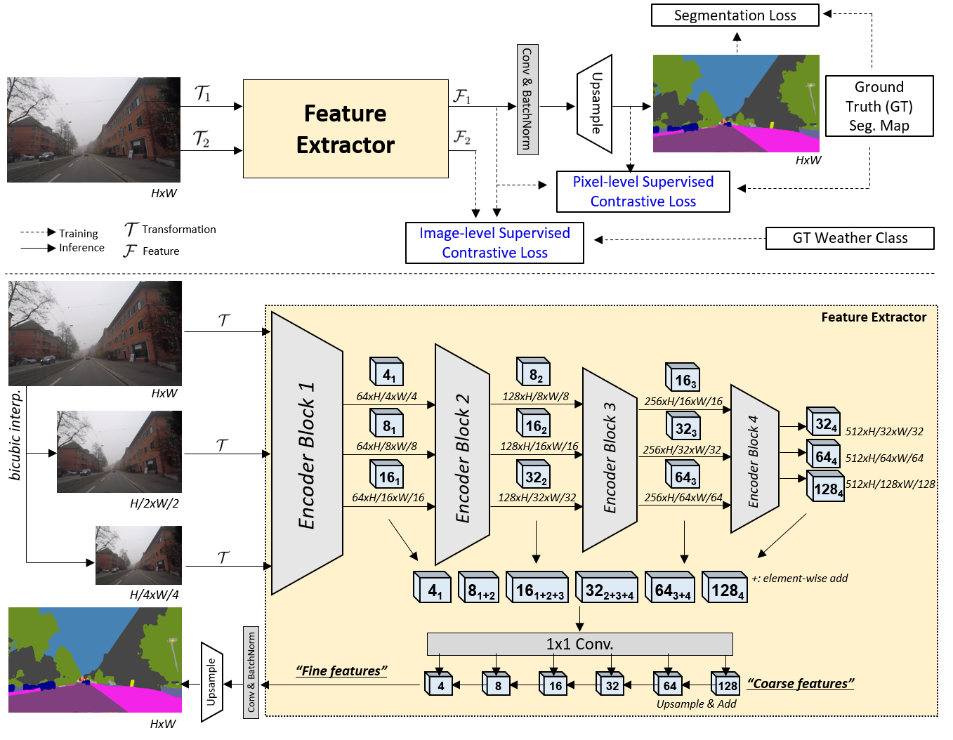
Figure 1: Overview of the training pipeline (top) and SwiftNet architecture (bottom).

We remark that our approach as shown in Fig. 1 is, in fact, also applicable to other supervised semantic segmentation tasks in which we have available ground truth pixel-level semantic labels as well as the corresponding image-level labels for those pixels in each image. Adverse weather conditions is one such case where we can readily acquire and exploit image-level contexts to promote contextual contrastive learning under unfavorable outdoor weather conditions.

The base model for our experiments is SwiftNet [Oršić and Šegvić(2021)] with the ResNet-18 backbone to balance the trade-off between the accuracy and the scale of model parameters and computations. SwiftNet is advantageous for its light weight and effectiveness in self-driving scenarios that often require real-time inference speed as well as comparably high performance to those of large-scale models [Song et al.(2022)Song, Jeong, and Kim]. Moreover, its multi-scale pyramidal features extracted from the sequential encoder blocks provide scale-invariant features that capture spatial information more precisely than single-scale models [Kim et al.(2018)Kim, Kook, Sun, Kang, and Ko].

Loss objective.  Standard semantic segmentation networks have long been trained according to the pixel-wise CE loss given class-specific probability distributions by weighting all pixels equally and considering the frequency of pixels belonging to each class [Oršić and Šegvić(2021), Zhang et al.(2019)Zhang, Liu, Wang, Lei, and Lu]. This approach, however, is prone to overfitting and biased towards more frequent classes. In addition, the CE loss suffers from failing to recognize edges in pixel-level granularity. To remedy these problems, [Lin et al.(2017)Lin, Goyal, Girshick, He, and Dollár, Oršić and Šegvić(2021)] have employed class balancing by adopting a scaling coefficient term to weight each class in a less biased and balanced manner.

We thus follow [Song et al.(2022)Song, Jeong, and Kim] in order to weight the cross-entropy and the focal loss [Lin et al.(2017)Lin, Goyal, Girshick, He, and Dollár] with the class-balancing term as described in Eq. 4, where we take the inverse logarithm of the ratio of the frequency of each pixel appearance, $freq_{c}$, over the entire pixels in the dataset, $N_{p}$. We choose $\epsilon=1\times 10^{-1}$ for numerical stability. The Euclidean distance transform (EDT) [Felzenszwalb and Huttenlocher(2012)] serves to weight each pixel by the distances to the boundaries of other objects. That is, for each pixel $p$ in a given image grid $G_{H\times W}$, we compute the $L_{2}$ distance to the nearest unmasked pixel $q$, i.e., the closest valid pixel belonging to the set of classes, $C$ as in Eq. 3.2. With both EDT and class-balancing terms in effect, the pixels of smaller objects and object boundaries are weighted greater than more frequently seen pixels such as those of sky or road classes during training.

$$\mathcal{L}_{seg}\left(\phi(p),\hat{\phi}(p)\right)=-\delta(p)e^{\gamma(1-P_{t})}log(P_{t}),$$ (4)

with

$$\delta(p)=\underbrace{log\left(1+\epsilon+\frac{freq_{c}(p)}{N_{p}}\right)^{-1}}_{\text{Class balancing}}\cdot\underbrace{exp\left(-\frac{d_{EDT}(p)}{2\sigma_{EDT}}\right)}_{\text{EDT}},$$

$$d_{EDT}(p)=\sum_{C}\min_{q\in C}\left\lVert p-q\right\rVert_{2}\quad\quad\quad\forall p\in G_{H\times W},\\$$

where $P_{t}$ denotes the softmax probability for each semantic class, and $\phi(p)$ and $\hat{\phi}(p)$ are the ground truth and the predicted segmentation maps, respectively. We then combine the segmentation and the contrastive loss terms as the final loss objective as follows:

$$\mathcal{L}=\lambda_{c}\cdot(\mathcal{L}_{\text{image}}+\mathcal{L}_{\text{pixel}})+\lambda_{s}\cdot\mathcal{L}_{seg},$$ (5)

where $\lambda_{c}=1/\mathcal{B}$, $\lambda_{s}=1.2$ and $\mathcal{B}$ is the batch size. For $\mathcal{L}_{image}$ and $\mathcal{L}_{pixel}$, we further add stability during training by adding $L_{2}$ normalization to the inner product (i.e., $\lVert\mathbf{z}_{i}\cdot\mathbf{z}_{p}\rVert_{2}$) to directly mimic the cosine similarity. The scaling coefficients, $\lambda_{c}$ and $\lambda_{s}$, are experimentally determined so as to reduce the unfavorable effect of feature equivalence matching and place a greater weight upon the segmentation objective. We also scale the contrastive loss value empirically to be close to the segmentation loss value. In this combined objective, the image-level contrast complements the pixel-level contrast such that the semantic correlations among intra-image pixels of each image are consistent across images of different weather classes globally without a memory bank. For the following experiments that use self-supervision in place of image-level contrast, we simply replace $\mathcal{L}_{image}$ with $\mathcal{L}_{self}$.

4 Experiments

4.1 Datasets and Evaluation Metric

We evaluate the proposed method using the training and validation sets of an urban street scene dataset, the Adverse Conditions Dataset with Correspondences for Semantic Driving Scene Understanding (ACDC) [Sakaridis et al.(2021)Sakaridis, Dai, and Van Gool], with and without pre-training on another driving scene benchmark dataset, the Cityscapes [Cordts et al.(2016)Cordts, Omran, Ramos, Rehfeld, Enzweiler, Benenson, Franke, Roth, and Schiele] as described in Table 1.

Cityscapes is a road scene benchmark dataset containing stereo RGB images taken from the egocentric point of view of the driver under clear, daytime weather, with pixel-level annotations for 19 semantic classes of various roadside objects including bus and fence. ACDC is a smaller dataset labelled according to the Cityscapes categories, yet in adverse conditions (fog, nighttime, rain and snow). While other Cityscapes-like datasets [Sakaridis et al.(2018)Sakaridis, Dai, and Van Gool, Dai et al.(2020)Dai, Sakaridis, Hecker, and Van Gool, Sakaridis et al.(2019)Sakaridis, Dai, and Van Gool, Zendel et al.(2018)Zendel, Honauer, Murschitz, Steininger, and Dominguez, Dai and Van Gool(2018), Yu et al.(2020)Yu, Chen, Wang, Xian, Chen, Liu, Madhavan, and Darrell, Tung et al.(2017)Tung, Chen, Meng, and Little] contain few to several hundred images biased toward specific adverse conditions, ACDC offers evenly-balanced number of images and the corresponding labels.

We evaluate the semantic segmentation performance by the mean Intersection-over-Union (IoU), also known as the Jaccard Index. IoU is often computed using the confusion matrix, from which we obtain true positive (TP), false positive (FP) and false negative (FN) scores for the predictions on the validation set, i.e., IoU = TP / (TP+FP+FN). The average IoU score computed over all fine category labels is denoted by mIoU, neglecting the void label.

Table 1: Dataset Description

Dataset	Input Modality	Resolution	Anno. (# Classes)	Weather Condition	Train	Val	Test
Cityscapes [Cordts et al.(2016)Cordts, Omran, Ramos, Rehfeld, Enzweiler, Benenson, Franke, Roth, and Schiele]	Stereo RGB	2048$\times$1024	Fine (19)	Clear/Daytime	2,975	500	1,525
ACDC [Sakaridis et al.(2021)Sakaridis, Dai, and Van Gool]	Monocular RGB	1920$\times$1080	Fine (19)	All	1,600	406	2,000
				Fog	400	100	500
				Nighttime	400	106	500
				Rain	400	100	500
				Snow	400	100	500

4.2 Implementation Details

We performed our experiments on a single Nvidia RTX 3090 GPU with PyTorch 1.7.1, CUDA 11.1, and CUDNN 8.3.2. In order to account for scale variations, we augmented the data with the following transformation: random square crop (768$\times$768) followed by scaling by a random value sampled from a uniform distribution$\sim$$U(0.5,2.0)$. We did not apply transformations that could potentially harm the image quality in adverse weather conditions such as color jitter. We set the validation image width and height to those of Cityscapes (2048$\times$1024) for fair comparison of the segmentation results. We pre-trained each model with ImageNet [Russakovsky et al.(2015)Russakovsky, Deng, Su, Krause, Satheesh, Ma, Huang, Karpathy, Khosla, Bernstein, Berg, and Fei-Fei] and set $\gamma=0.5$ in the focal loss, the temperature $\tau=0.07$, and the feature dimension to $D_{proj}=128$ for the supervised contrast. We trained the network on the ACDC dataset for 400 epochs with a batch size of 8, using an Adam [Kingma and Ba(2014)] optimizer with $\beta_{1}=0.9$, $\beta_{2}=0.99$. We set the initial learning rate and the weight decay to $4\times 10^{-4}$ and $1\times 10^{-4}$, respectively, and used a cosine annealing scheduler to decay the learning rate to $1\times 10^{-6}$ in the last epoch.

4.3 Evaluation

Quantitative results.  We summarize the semantic segmentation results in Table 2, where there are 1.34%p and 1.33%p increases in mIoU from the baseline for the ResNet-18 and -34 backbones, respectively, for our method. Our proposed method generally outperforms in mIoU under each of the four adverse conditions, relative to the other experimented single and double contrasts. Our method is particularly effective for the harder conditions, namely nighttime, rain and snow, where we exploit the semantic correlations in the embeddings across the pixels of different conditions owing to the doubly contrastive objective. We remark that the difficulties in predictions in nighttime and rain stem from a significant number of darker pixels obstructing clear view of objects in the driving area and rain droplets distorting the camera view and the texture of objects at far distances, respectively. The performance under fog is not relatively lower than in clear weather due to low fog density. Further, we highlight that our experiments are accompanied with a batch size of 8 under a more practical training scenario. We expect higher performance gain with a batch size of 2048 as suggested in common contrastive learning works [Khosla et al.(2020)Khosla, Teterwak, Wang, Sarna, Tian, Isola, Maschinot, Liu, and Krishnan].

With pre-training on clear weather images, there are 0.86%p and 1.80%p improvement in mIoU for the ResNet-18 and -34 backbones for our method, respectively, after fine-tuning on the adverse weather images. Note that the experiment (f) achieves as high overall mIoU as the experiment (g), as well as in each weather-specific mIoU score. While our method has minor improvements for all conditions except fog with the ResNet-18, we observed noticeable increases with the ResNet-18 backbones.

Qualitative results.  As shown in Fig. 2, our doubly contrastive method corrects false positive predictions from the focal loss (baseline) case, and allows to predict objects of a relatively large size more consistently. For instance, it removes noisy predictions on road, removes the fuzzy boundary between road and sidewalk, and fills in mis-classified pixels with the correct label for somewhat noisily predicted objects. Specifically in rain, it recovers a pole that seemed nonexistent in the baseline and corrects the pixels mis-classified as sidewalk to road. The effect of our method is more apparent when there is a region with a majority of pixels belonging to a single class, yet there remains mis-classified or noisy pixels in part.

Table 2: Semantic segmentation performance by adverse weather conditions using SwiftNet. Bb denotes backbone. The best results in boldface and the second best in underline.

Bb	Exp.	Loss (∗: single contrast, †: double contrasts)	mIoU (%)	Fog	Nighttime	Rain	Snow
ResNet-18	(a)	Cross Entropy	62.63	68.95	45.71	63.32	65.43
	(b)	Focal (baseline)	64.04	71.59	47.84	63.90	65.57
	(c)	+Pixel-level Supervised Contrast only∗	63.79	69.76	47.26	63.05	68.34
	(d)	+Self-supervised Contrast only∗	63.91	71.83	48.02	62.24	68.35
	(e)	+Image-level Supervised Contrast only∗	63.62	69.66	47.65	63.28	67.10
	(f)	+Self-supervised and Pixel-level Supervised Contrasts†	65.07	72.45	48.57	63.95	68.31
	(g)	+Image- and Pixel-level Supervised Contrasts† (Ours)	65.38	67.94	48.56	65.38	68.64
ResNet-34	(a)	Cross Entropy	65.02	73.85	47.11	65.20	66.94
	(b)	Focal (baseline)	67.00	74.44	49.38	67.29	70.64
	(c)	+Pixel-level Supervised Contrast only∗	66.60	72.49	49.84	65.55	69.06
	(d)	+Self-supervised Contrast only∗	68.09	76.99	50.14	66.45	69.56
	(e)	+Image-level Supervised Contrast only∗	68.07	75.12	50.76	66.78	69.33
	(f)	+Self-supervised and Pixel-level Supervised Contrasts†	67.02	72.06	50.12	65.86	70.83
	(g)	+Image- and Pixel-level Supervised Contrasts† (Ours)	68.33	75.19	51.21	67.37	71.19
Bb	Exp.	Loss (w/ pre-training with clear weather)	mIoU (%)	Fog	Nighttime	Rain	Snow
ResNet-18	-	Focal (Cityscapes)	73.16	N/A (Clear weather only)
	(a)	Cross Entropy	64.40	71.88	47.09	65.59	66.66
	(b)	Focal (baseline)	65.49	73.43	47.67	64.77	68.35
	(f)	+Self-supervised and Pixel-level Supervised Contrasts†	66.97	74.05	49.10	67.85	69.69
	(g)	+Image- and Pixel-level Supervised Contrasts (Ours)†	66.24	75.38	48.82	65.79	68.42
ResNet-34	-	Focal (Cityscapes)	73.80	N/A (Clear weather only)
	(a)	Cross Entropy	68.38	75.99	49.70	67.92	71.49
	(b)	Focal (baseline)	69.46	76.94	50.28	69.78	71.69
	(f)	+Self-supervised and Pixel-level Supervised Contrasts†	70.06	76.11	50.47	70.68	72.89
	(g)	+Image- and Pixel-level Supervised Contrasts (Ours)†	70.13	76.31	53.59	70.50	71.89

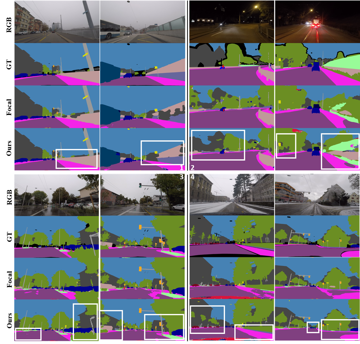
Figure 2: Two samples of semantic segmentation prediction results for each of the four weather conditions: fog, night, rain and snow (1 $\rightarrow$ 4). Please zoom in to see details.

Feature visualization.

Figure 3: t-SNE visualizations for the trained features using SwiftNet (ResNet-18). Top row: focal loss only (baseline). Bottom row: Ours. Columns from left to right: weather class-wise features, and pixel-wise features for fog, nighttime, rain and snow, in order. Void class is not shown. Please zoom in to see details.

For an in-depth analysis of the learned features, we provide the class- and pixel-wise t-SNE visualizations for the baseline and our method in Fig. 3. For the class-wise features categorized into the four weather conditions, our doubly contrastive method better discriminates images of the fog and night classes from images of the other two. Images of these two categories are more clustered and densely located by themselves.

For pixel-wise features, we opted to visualize for the first batch of pixel-wise feature embeddings due to a memory contraint, where we observed that the features are more densely populated, thereby appearing darker in each respective color. This insinuates pixels belonging to the same class are more compactly located in the feature space. While grouping patterns seem more apparent for the baseline, our combination of image- and pixel-level supervised contrastive objectives finds a good balance in the feature space that yields higher semantic segmentation scores.

Ablation studies.  We examine the effect of different feature extractors as well as the fine vs. coarse feature granularity as noted in Fig. 1. Table 3 presents the results and the corresponding computational costs when the SwiftNet feature extractor is replaced by that of ENet and DeepLabV3+ (ResNet-50 backbone). While our method is effective with SwiftNet, it is not as effective as with ENet or with DeepLabV3+. We infer that this is due to the single-scale encoder for ENet, and the ASPP module for DeepLabV3+. While SwiftNet draws multi-resolution features sequentially from the previous scale features, DeepLabV3+ applies convolutions with different kernel sizes and pools altogether in one step. We applied our image-level contrast to the ENet features before upsampling and DeepLabV3+ features after ASPP followed by 1$\times$1 convolution, respectively. In terms of memory, ENet is the smallest in size, yet it requires heavy memory space and is thus relatively slower. DeepLabV3+, on the other hand, is large in size even with ResNet-50 instead of its proposed Xception-71. Replacing the fine features with the coarse in SwiftNet yields a drop of 3.75%p in mIoU for our method since fine features contain the fused output from the features from multi-resolution encoder blocks that provide geometrically richer contexts than the coarse.

Table 3: Ablation study: semantic segmentation performance with different models and coarse features (2048$\times$1024 resolution). Coarse features are marked with ${\dagger}$; otherwise fine.

Model (Encoder type)	Exp.	mIoU (%)	Fog	Nighttime	Rain	Snow	GFLOPs	Params (M)	RTX 3080 Mobile
									Time (ms)	FPS
	(a)	45.22	48.10	36.31	44.46	47.53	1.40	0.35	31	32.3
ENet [Paszke et al.(2016)Paszke, Chaurasia, Kim, and Culurciello]	(b)	50.45	55.14	38.70	49.44	53.44
(Single-scale)	(f)	50.78	55.91	38.96	50.88	52.39
	(g)	49.32	53.64	37.85	49.86	51.17
	(a)	62.63	68.95	45.71	63.32	65.43	8.04	12.04	15	66.7
	(b)	64.04	71.59	47.84	63.90	65.57
SwiftNet (ResNet-18) [Oršić and Šegvić(2021)]	(f)	65.07	72.45	48.57	63.95	68.31
(Multi-scale pyramidal)	(g)	65.38	67.94	48.56	65.38	68.64
	(f)†	60.62	65.84	45.35	61.20	64.79
	(g)†	61.66	67.86	46.07	62.10	64.84
	(a)	65.02	73.85	47.11	65.20	66.94	14.40	22.15	26	38.5
SwiftNet (ResNet-34) [Oršić and Šegvić(2021)]	(b)	67.00	74.44	49.38	67.29	70.64
(Multi-scale pyramidal)	(f)	67.02	72.06	50.12	65.86	70.83
	(g)	68.33	75.19	51.21	67.37	71.19
	(a)	69.69	73.60	51.45	72.18	72.29	29.88	39.76	14	71.4
DeepLabV3+ (ResNet-50) [Chen et al.(2018)Chen, Zhu, Papandreou, Schroff, and Adam]	(b)	70.07	75.18	52.49	73.22	71.50
(ASPP)	(f)	69.22	73.95	50.54	70.42	73.24
	(g)	69.04	74.54	51.20	70.70	71.83

5 Conclusion

We proposed an end-to-end doubly contrastive learning approach to semantic segmentation for self-driving under adverse weather. Our doubly contrastive method exploits image-level labels to semantically correlate RGB images taken under various weather conditions and pixel-level labels to obtain more semantically meaningful representations. In our method, the two supervised contrasts complement each other to effectively improve the performance of a lightweight model, without a need for pre-training or a memory bank to associate images across various weather conditions for global consistency. We hope this sheds further light on contrastive learning approaches for real-time deployment of self-driving systems.

Acknowledgments.  This work was supported by the Institute for Information & Communications Technology Promotion (IITP) under Grant 2020-0-00440 through the Korean Government (Ministry of Science and ICT (MSIT); Development of Artificial Intelligence Technology that Continuously Improves Itself as the Situation Changes in the Real World).

References

- [Ahn and Kwak(2018)] Jiwoon Ahn and Suha Kwak. Learning pixel-level semantic affinity with image-level supervision for weakly supervised semantic segmentation. In Proceedings of the IEEE conference on computer vision and pattern recognition, pages 4981–4990, 2018.
- [Alonso et al.(2021)Alonso, Sabater, Ferstl, Montesano, and Murillo] Inigo Alonso, Alberto Sabater, David Ferstl, Luis Montesano, and Ana C Murillo. Semi-supervised semantic segmentation with pixel-level contrastive learning from a class-wise memory bank. In Proceedings of the IEEE/CVF International Conference on Computer Vision, pages 8219–8228, 2021.
- [Andrey and Yagar(1993)] Jean Andrey and Sam Yagar. A temporal analysis of rain-related crash risk. Accident Analysis & Prevention, 25(4):465–472, 1993. ISSN 0001-4575. https://doi.org/10.1016/0001-4575(93)90076-9. URL https://www.sciencedirect.com/science/article/pii/0001457593900769.
- [Badrinarayanan et al.(2017)Badrinarayanan, Kendall, and Cipolla] Vijay Badrinarayanan, Alex Kendall, and Roberto Cipolla. Segnet: A deep convolutional encoder-decoder architecture for image segmentation. IEEE transactions on pattern analysis and machine intelligence, 39(12):2481–2495, 2017.
- [Becker and Hinton(1992)] Suzanna Becker and Geoffrey E Hinton. Self-organizing neural network that discovers surfaces in random-dot stereograms. Nature, 355(6356):161–163, 1992.
- [Berthelot et al.(2019)Berthelot, Carlini, Goodfellow, Papernot, Oliver, and Raffel] David Berthelot, Nicholas Carlini, Ian Goodfellow, Nicolas Papernot, Avital Oliver, and Colin A Raffel. Mixmatch: A holistic approach to semi-supervised learning. Advances in Neural Information Processing Systems, 32, 2019.
- [Chen et al.(2018)Chen, Zhu, Papandreou, Schroff, and Adam] Liang-Chieh Chen, Yukun Zhu, George Papandreou, Florian Schroff, and Hartwig Adam. Encoder-decoder with atrous separable convolution for semantic image segmentation. In Proceedings of the European conference on computer vision (ECCV), pages 801–818, 2018.
- [Chen et al.(2020a)Chen, Kornblith, Norouzi, and Hinton] Ting Chen, Simon Kornblith, Mohammad Norouzi, and Geoffrey Hinton. A simple framework for contrastive learning of visual representations. In International conference on machine learning, pages 1597–1607. PMLR, 2020a.
- [Chen et al.(2020b)Chen, Kornblith, Swersky, Norouzi, and Hinton] Ting Chen, Simon Kornblith, Kevin Swersky, Mohammad Norouzi, and Geoffrey E Hinton. Big self-supervised models are strong semi-supervised learners. Advances in neural information processing systems, 33:22243–22255, 2020b.
- [Cordts et al.(2016)Cordts, Omran, Ramos, Rehfeld, Enzweiler, Benenson, Franke, Roth, and Schiele] Marius Cordts, Mohamed Omran, Sebastian Ramos, Timo Rehfeld, Markus Enzweiler, Rodrigo Benenson, Uwe Franke, Stefan Roth, and Bernt Schiele. The cityscapes dataset for semantic urban scene understanding. In Proceedings of the IEEE conference on computer vision and pattern recognition, pages 3213–3223, 2016.
- [Dai and Van Gool(2018)] Dengxin Dai and Luc Van Gool. Dark model adaptation: Semantic image segmentation from daytime to nighttime. In IEEE International Conference on Intelligent Transportation Systems, 2018.
- [Dai et al.(2020)Dai, Sakaridis, Hecker, and Van Gool] Dengxin Dai, Christos Sakaridis, Simon Hecker, and Luc Van Gool. Curriculum model adaptation with synthetic and real data for semantic foggy scene understanding. International Journal of Computer Vision, 128(5):1182–1204, 2020.
- [Doersch and Zisserman(2017)] Carl Doersch and Andrew Zisserman. Multi-task self-supervised visual learning. In Proceedings of the IEEE International Conference on Computer Vision, pages 2051–2060, 2017.
- [Federal Motor Carrier Safety Administration()] Federal Motor Carrier Safety Administration. Code of federal regulations. Accessed May 23, 2022 [Online]. URL https://www.ecfr.gov/cgi-bin/retrieveECFR?gp=1&ty=HTML&h=L&mc=true&=PART&n=pt49.5.395#se49.5.395_12.
- [Felzenszwalb and Huttenlocher(2012)] Pedro F Felzenszwalb and Daniel P Huttenlocher. Distance transforms of sampled functions. Theory of computing, 8(1):415–428, 2012.
- [Gidaris et al.(2018)Gidaris, Singh, and Komodakis] Spyros Gidaris, Praveer Singh, and Nikos Komodakis. Unsupervised representation learning by predicting image rotations. arXiv preprint arXiv:1803.07728, 2018.
- [Gutmann and Hyvärinen(2010)] Michael Gutmann and Aapo Hyvärinen. Noise-contrastive estimation: A new estimation principle for unnormalized statistical models. In Proceedings of the thirteenth international conference on artificial intelligence and statistics, pages 297–304. JMLR Workshop and Conference Proceedings, 2010.
- [He et al.(2016)He, Zhang, Ren, and Sun] Kaiming He, Xiangyu Zhang, Shaoqing Ren, and Jian Sun. Deep residual learning for image recognition. In Proceedings of the IEEE conference on computer vision and pattern recognition, pages 770–778, 2016.
- [Khan et al.(2021)Khan, Kim, and Chua] Abbas Khan, Hyongsuk Kim, and Leon Chua. Pmed-net: Pyramid based multi-scale encoder-decoder network for medical image segmentation. IEEE Access, 9:55988–55998, 2021. 10.1109/ACCESS.2021.3071754.
- [Khosla et al.(2020)Khosla, Teterwak, Wang, Sarna, Tian, Isola, Maschinot, Liu, and Krishnan] Prannay Khosla, Piotr Teterwak, Chen Wang, Aaron Sarna, Yonglong Tian, Phillip Isola, Aaron Maschinot, Ce Liu, and Dilip Krishnan. Supervised contrastive learning. Advances in Neural Information Processing Systems, 33:18661–18673, 2020.
- [Kim et al.(2018)Kim, Kook, Sun, Kang, and Ko] Seung-Wook Kim, Hyong-Keun Kook, Jee-Young Sun, Mun-Cheon Kang, and Sung-Jea Ko. Parallel feature pyramid network for object detection. In Proceedings of the European Conference on Computer Vision (ECCV), pages 234–250, 2018.
- [Kingma and Ba(2014)] Diederik P Kingma and Jimmy Ba. Adam: A method for stochastic optimization. arXiv preprint arXiv:1412.6980, 2014.
- [Lin et al.(2017)Lin, Goyal, Girshick, He, and Dollár] Tsung-Yi Lin, Priya Goyal, Ross Girshick, Kaiming He, and Piotr Dollár. Focal loss for dense object detection. In Proceedings of the IEEE international conference on computer vision, pages 2980–2988, 2017.
- [Long et al.(2015)Long, Shelhamer, and Darrell] Jonathan Long, Evan Shelhamer, and Trevor Darrell. Fully convolutional networks for semantic segmentation. In Proceedings of the IEEE conference on computer vision and pattern recognition, pages 3431–3440, 2015.
- [Noh et al.(2015)Noh, Hong, and Han] Hyeonwoo Noh, Seunghoon Hong, and Bohyung Han. Learning deconvolution network for semantic segmentation. In Proceedings of the IEEE international conference on computer vision, pages 1520–1528, 2015.
- [Noroozi and Favaro(2016)] Mehdi Noroozi and Paolo Favaro. Unsupervised learning of visual representations by solving jigsaw puzzles. In European conference on computer vision, pages 69–84. Springer, 2016.
- [Organization(2021)] World Health Organization. Road traffic injuries, 2021. URL https://www.who.int/news-room/fact-sheets/detail/road-traffic-injuries.
- [Oršić and Šegvić(2021)] Marin Oršić and Siniša Šegvić. Efficient semantic segmentation with pyramidal fusion. Pattern Recognition, 110:107611, 2021.
- [Paszke et al.(2016)Paszke, Chaurasia, Kim, and Culurciello] Adam Paszke, Abhishek Chaurasia, Sangpil Kim, and Eugenio Culurciello. Enet: A deep neural network architecture for real-time semantic segmentation. CoRR, abs/1606.02147, 2016. URL http://arxiv.org/abs/1606.02147.
- [Pinheiro and Collobert(2015)] Pedro O Pinheiro and Ronan Collobert. From image-level to pixel-level labeling with convolutional networks. In Proceedings of the IEEE conference on computer vision and pattern recognition, pages 1713–1721, 2015.
- [Ronneberger et al.(2015)Ronneberger, Fischer, and Brox] Olaf Ronneberger, Philipp Fischer, and Thomas Brox. U-net: Convolutional networks for biomedical image segmentation. In International Conference on Medical image computing and computer-assisted intervention, pages 234–241. Springer, 2015.
- [Russakovsky et al.(2015)Russakovsky, Deng, Su, Krause, Satheesh, Ma, Huang, Karpathy, Khosla, Bernstein, Berg, and Fei-Fei] Olga Russakovsky, Jia Deng, Hao Su, Jonathan Krause, Sanjeev Satheesh, Sean Ma, Zhiheng Huang, Andrej Karpathy, Aditya Khosla, Michael Bernstein, Alexander C. Berg, and Li Fei-Fei. ImageNet Large Scale Visual Recognition Challenge. International Journal of Computer Vision (IJCV), 115(3):211–252, 2015. 10.1007/s11263-015-0816-y.
- [Sakaridis et al.(2018)Sakaridis, Dai, and Van Gool] Christos Sakaridis, Dengxin Dai, and Luc Van Gool. Semantic foggy scene understanding with synthetic data. International Journal of Computer Vision, 126(9):973–992, Sep 2018. URL https://doi.org/10.1007/s11263-018-1072-8.
- [Sakaridis et al.(2019)Sakaridis, Dai, and Van Gool] Christos Sakaridis, Dengxin Dai, and Luc Van Gool. Guided curriculum model adaptation and uncertainty-aware evaluation for semantic nighttime image segmentation. In The IEEE International Conference on Computer Vision (ICCV), 2019.
- [Sakaridis et al.(2021)Sakaridis, Dai, and Van Gool] Christos Sakaridis, Dengxin Dai, and Luc Van Gool. ACDC: The adverse conditions dataset with correspondences for semantic driving scene understanding. In Proceedings of the IEEE/CVF International Conference on Computer Vision (ICCV), October 2021.
- [Song et al.(2022)Song, Jeong, and Kim] Taek-Jin Song, Jongoh Jeong, and Jong-Hwan Kim. End-to-end real-time obstacle detection network for safe self-driving via multi-task learning. IEEE Transactions on Intelligent Transportation Systems, pages 1–12, 2022. 10.1109/TITS.2022.3149789.
- [Tung et al.(2017)Tung, Chen, Meng, and Little] Frederick Tung, Jianhui Chen, Lili Meng, and James J Little. The raincouver scene parsing benchmark for self-driving in adverse weather and at night. IEEE Robotics and Automation Letters, 2(4):2188–2193, 2017.
- [Valada et al.(2017)Valada, Vertens, Dhall, and Burgard] Abhinav Valada, Johan Vertens, Ankit Dhall, and Wolfram Burgard. Adapnet: Adaptive semantic segmentation in adverse environmental conditions. In 2017 IEEE International Conference on Robotics and Automation (ICRA), pages 4644–4651. IEEE, 2017.
- [Van den Oord et al.(2018)Van den Oord, Li, and Vinyals] Aaron Van den Oord, Yazhe Li, and Oriol Vinyals. Representation learning with contrastive predictive coding. arXiv e-prints, pages arXiv–1807, 2018.
- [Wang et al.(2020)Wang, Sun, Cheng, Jiang, Deng, Zhao, Liu, Mu, Tan, Wang, et al.] Jingdong Wang, Ke Sun, Tianheng Cheng, Borui Jiang, Chaorui Deng, Yang Zhao, Dong Liu, Yadong Mu, Mingkui Tan, Xinggang Wang, et al. Deep high-resolution representation learning for visual recognition. IEEE transactions on pattern analysis and machine intelligence, 43(10):3349–3364, 2020.
- [Wang et al.(2021)Wang, Zhou, Yu, Dai, Konukoglu, and Van Gool] Wenguan Wang, Tianfei Zhou, Fisher Yu, Jifeng Dai, Ender Konukoglu, and Luc Van Gool. Exploring cross-image pixel contrast for semantic segmentation. In Proceedings of the IEEE/CVF International Conference on Computer Vision, pages 7303–7313, 2021.
- [Xie et al.(2020)Xie, Dai, Hovy, Luong, and Le] Qizhe Xie, Zihang Dai, Eduard Hovy, Thang Luong, and Quoc Le. Unsupervised data augmentation for consistency training. Advances in Neural Information Processing Systems, 33:6256–6268, 2020.
- [Xu et al.(2015)Xu, Schwing, and Urtasun] Jia Xu, Alexander G Schwing, and Raquel Urtasun. Learning to segment under various forms of weak supervision. In Proceedings of the IEEE conference on computer vision and pattern recognition, pages 3781–3790, 2015.
- [Yu et al.(2020)Yu, Chen, Wang, Xian, Chen, Liu, Madhavan, and Darrell] Fisher Yu, Haofeng Chen, Xin Wang, Wenqi Xian, Yingying Chen, Fangchen Liu, Vashisht Madhavan, and Trevor Darrell. Bdd100k: A diverse driving dataset for heterogeneous multitask learning. In Proceedings of the IEEE/CVF conference on computer vision and pattern recognition, pages 2636–2645, 2020.
- [Zendel et al.(2018)Zendel, Honauer, Murschitz, Steininger, and Dominguez] Oliver Zendel, Katrin Honauer, Markus Murschitz, Daniel Steininger, and Gustavo Fernandez Dominguez. Wilddash-creating hazard-aware benchmarks. In Proceedings of the European Conference on Computer Vision (ECCV), pages 402–416, 2018.
- [Zhang et al.(2019)Zhang, Liu, Wang, Lei, and Lu] Pingping Zhang, Wei Liu, Hongyu Wang, Yinjie Lei, and Huchuan Lu. Deep gated attention networks for large-scale street-level scene segmentation. Pattern Recognition, 88:702–714, 2019.
- [Zhao et al.(2018)Zhao, Qi, Shen, Shi, and Jia] Hengshuang Zhao, Xiaojuan Qi, Xiaoyong Shen, Jianping Shi, and Jiaya Jia. Icnet for real-time semantic segmentation on high-resolution images. In Proceedings of the European conference on computer vision (ECCV), pages 405–420, 2018.