Quantum theory of light-driven coherent lattice dynamics

Abstract

The exposure to intense electromagnetic radiation can induce distortions and symmetry breaking in the crystal structure of solids, providing a route for the all-optical control of their properties. In this manuscript, we formulate a unified theoretical approach to describe the coherent lattice dynamics in presence of external driving fields, electron-phonon and phonon-phonon interactions, and quantum nuclear effects. The main mechanisms for the excitation of coherent phonons – including infrared absorption, displacive excitation, inelastic stimulated Raman scattering, and ionic Raman scattering – can be seamlessly accounted for. We apply this formalism to a model consisting of two coupled phonon modes, where we illustrate the influence of quantum nuclei on structural distortions induced by ionic Raman scattering. Besides validating the widely-employed classical models for the coherent lattice dynamics, our work provides a versatile approach to methodically explore the emergence of quantum nuclear effects in the structural response of crystal lattice to strong fields.

I Introduction

The structural dynamics of solids triggered by intense light pulses [1] can act as a precursor for driving materials across phase transitions [2] or into metastable states inaccessible in equilibrium conditions [3]. Besides the fundamental importance of this route for light-assisted structural control, numerous domains of application where these concepts could be of technological relevance can be easily envisioned. Experimental realizations of this paradigm are numerous and include the all-optical switching of electric polarization in ferroelectrics [4, 3, 5], insulator to metal transitions [6], enhanced superconductivity [7, 8, 9], or the tuning of spin dynamics [10] and magnetism [11, 12, 13, 14, 15, 16]. A review of the recent progress in exploring and exploiting light-induced structural control and related phenomena in matter can be found in Refs. [2, 17].

The non-equilibrium dynamics of the crystalline lattice triggered by light absorption consists simultaneously of incoherent and coherent parts. The incoherent lattice dynamics is characterized by the increase in phonon population of the phonon modes directly coupled to the field as, for example, infrared (IR) active modes driven by absorption of a terahertz (THz) field. As schematically illustrated in Fig. 1 (a), this mechanism is equivalent to the excitation of the quantum harmonic oscillator upon absorption of a photon. The coherent dynamics, conversely, is linked to the displacement of the nuclear wave packets from their equilibrium positions [Fig. 1 (b)], and it underpins the periodic motion of the nuclei around their thermal equilibrium positions [18, 19, 20, 21]. This behaviour is absent in a purely incoherent state of the lattice (e.g., at thermal equilibrium), where the nuclear vibrations depend on the phonon modes population plus the associated zero-point amplitude. Several coherent phonon excitation mechanism are discussed in the literature, including THz light pulses [21], impulsive stimulated Raman scattering (ISRS) [22, 20, 21, 23], ionic Raman scattering [24, 25, 26, 27], sum-frequency Raman scattering [28], and sum-frequency ionic Raman scattering [29].

A theoretical description of the incoherent lattice dynamics can be addressed, for instance, from the solution of the time-dependent Boltzmann equation (TDBE) for the lattice [30, 31] by accounting explicitly for coupling to external fields, as well as the scattering processes that drive the system towards thermalization (electron-electron, electron-phonon, phonon-phonon). In the TDBE formalism, the non-equilibrium lattice dynamics is approximately described by the time-dependent changes of the phonon occupations arising from external perturbations [32]. Overall, the TDBE suffices to describe the non-equilibrium variations of phonon occupations [Fig. 1 (a)] associated with the incoherent dynamics [33, 34], however, it is inherently unsuitable to account for coherent structural dynamics.

If the quantum nature of the nuclei is neglected, the coherent lattice dynamics in presence of external driving fields can be formulated within the framework of classical mechanics [35] and recast in the form of a driven harmonic oscillator equation of motion (EOM), which admits a numerical or analytical solution. Classical models have seen wide application in the domain of light-driven structural control [36, 7, 37, 38, 39, 40, 41, 11, 29, 42, 3, 43, 44], and they have proven suitable and predictive in describing physical phenomena in which the structural dynamics can be attributed to two or few coupled phonons. A limitation of driven harmonic oscillator models is that they rely on a classical description of nuclear motion, which makes them unsuitable to assess the influence of quantum nuclear effects on the coherent lattice dynamics. Additionally, in their most common implementations, only lattice dynamics in the unit cell is considered although this can be circumvented within a supercell approach. Quantum effects can play a substantial role in the nuclear dynamics at low temperatures and/or in compounds with light atoms (e.g., H and Li) [45, 46]; the emergence of long-range order (e.g. charge-density waves, disorder, or domain formation) are inherently linked to the structural dynamics on length scales beyond the unit cell.

Ab-initio molecular dynamics (AIMD) circumvents some of the limitations mentioned above. It can be extended to account for coupling to external driving fields fully ab initio [47]; it accounts for lattice anharmonicity up to all orders via the explicit calculation of the potential energy surface for each nuclear configuration; the influence of phonons with a finite wavevector on the dynamics can be encoded in the simulations by extending the size of simulation cells. However, AIMD remains inherently classical and it does not enable a simple inclusion of quantum nuclear effects. In earlier works, quantum nuclear effects have been accounted for within the framework of path-integral molecular dynamics [48], or via the introduction of suitable thermostats [49]. Additionally, AIMD simulations in supercells remain prohibitively expensive for all but the simplest systems. Overall, these considerations outline the limitations of existing theoretical approaches in the description of the light-driven structural control.

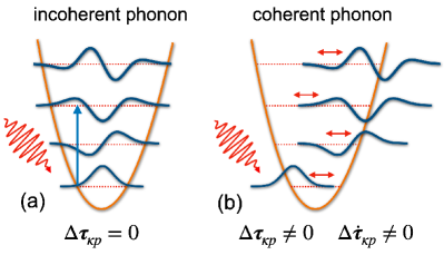
Figure 1: Schematic illustration of an incoherent (a) and coherent (b) phonon excitation. Incoherent phonons are determined by the quantum number of the harmonic oscillator $n_{{\bf q}\nu}$ and maintain a zero average displacement of the lattice ($\Delta{\bm{\tau}}_{\kappa p}=0$). Coherent phonons are characterized by the displacement of the nuclear wave packets from thermal equilibrium ($\Delta{\bm{\tau}}_{\kappa p}\neq 0$) induced by external perturbations which lead to a periodic motion of the nuclear wave packets ($\Delta\dot{\bm{\tau}}_{\kappa p}\neq 0$).

In this manuscript, we formulate a quantum theory of the light-induced coherent structural dynamics in solids. Our approach is based on the solution of the Heisenberg EOM for the nuclear coordinate operator, and allows for systematically including (i) the coupling to external fields radiation at linear order in the field intensity; (ii) quantum nuclear effects; (iii) lattice anharmonicities due to all phonons. We show that the classical models, widely employed in the field of non-linear phononics, can be recovered within this framework by neglecting quantum nuclear effects. To corroborate these considerations and explore the main features of the classical and quantum dynamics, we solve numerically the lattice EOM for a minimal model consisting of two phonons coupled by lattice anharmonicities and driven by a THz field.

The manuscript is organized as follows. In Sec. II we introduce the general Hamiltonian for a crystalline lattice. In Sec. III we discuss the TDBE and its application to the study of incoherent phonons. Section IV discusses a general approach to derive the coherent dynamics of solids based on the solution of the Heisenberg EOM for the nuclear displacement operator. Section V discusses the different forms of the coherent phonon driving forces. Section VI illustrates application to the coherent dynamics of a harmonic lattice interacting with a THz field. In Sec. VII the lattice dynamics in the presence of anharmonicities is discussed. In Sec. VIII we demonstrate the present formalism using a two-phonon model. Summary and conclusions are presented in Sec. IX.

II Ab-initio Lattice Hamiltonian

The Hamiltonian for an anharmonic lattice interacting with an electromagnetic field can be expressed as [50]:

$$\hat{H} =\hat{H}_{\rm ph}+\hat{H}_{\rm eph}+\hat{H}_{\rm pp}+\hat{H}_{\rm IR},$$ (1)

where $\hat{H}_{\rm ph}$, $\hat{H}_{\rm eph}$, $\hat{H}_{\rm pp}$, and $\hat{H}_{\rm IR}$ represent the Hamiltonian of the lattice in the harmonic approximation, the electron-phonon and phonon-phonon interaction Hamiltonians, and the Hamiltonian accounting for the coupling with the THz field, respectively. In second-quantization, $\hat{H}_{\rm ph}$ can be expressed as:

$$\hat{H}_{\rm ph} =\sum_{{\bf q}\nu}\hbar\omega_{{\bf q}\nu}(\hat{a}_{{\bf q}\nu}^{\dagger}\hat{a}_{{\bf q}\nu}+1/2)\quad.$$ (2)

Here, $\omega_{{\bf q}\nu}$ is the frequency of a phonon with momentum ${\bf q}$ and mode index $\nu$. The sum over ${\bf q}$ extends over crystal momenta in the Brillouin zone. $\hat{a}_{{\bf q}\nu}^{\dagger}$ and $\hat{a}_{{\bf q}\nu}$ are bosonic creation and annihilation operators, respectively, which obey the usual commutation relations. In the following, we find it convenient to introduce the shortened notation:

$$\hat{Q}_{{\bf q}\nu} =\hat{a}_{{\bf q}\nu}+\hat{a}^{\dagger}_{-{\bf q}\nu}\quad,$$ (3)

$$\hat{P}_{{\bf q}\nu} =\hat{a}_{{\bf q}\nu}-\hat{a}^{\dagger}_{-{\bf q}\nu}\quad.$$ (4)

The expectation values ${Q}_{{\bf q}\nu}=\langle\hat{Q}_{{\bf q}\nu}\rangle$ and ${P}_{{\bf q}\nu}=\langle\hat{P}_{{\bf q}\nu}\rangle$ yield the displacement amplitude and momentum for a coherent phonon with momentum ${{\bf q}}$ and index $\nu$. The commutation relations for $\hat{Q}_{{\bf q}\nu}$ and $\hat{P}_{{\bf q}\nu}$ are listed in Appendix A.

$\hat{H}_{\rm pp}$ is the phonon-phonon interaction Hamiltonian which accounts for anharmonicities of the lattice. Up to fourth order in the expansion of the potential energy surface with respect to the lattice displacements, $\hat{H}_{\rm pp}$ is given by:

$$\hat{H}_{\rm pp}=\frac{1}{3!}\sum_{{\bf q}{\bf q}^{\prime}{\bf q}^{\prime\prime}}\sum_{\nu\nu^{\prime}\nu^{\prime\prime}}\Psi^{(3)}_{\begin{subarray}{c}\nu\nu^{\prime}\nu^{\prime\prime}\\ {\bf q}{\bf q}^{\prime}{\bf q}^{\prime\prime}\end{subarray}}\hat{Q}_{{\bf q}\nu}\hat{Q}_{{\bf q}^{\prime}\nu^{\prime}}\hat{Q}_{{\bf q}^{\prime\prime}\nu^{\prime\prime}}$$ (5)

$$+\frac{1}{4!}\sum_{{\bf q}{\bf q}^{\prime}{\bf q}^{\prime\prime}{\bf q}^{\prime\prime\prime}}\sum_{\nu\nu^{\prime}\nu^{\prime\prime}\nu^{\prime\prime\prime}}\Psi^{(4)}_{\begin{subarray}{c}\nu\nu^{\prime}\nu^{\prime\prime}\nu^{\prime\prime\prime}\\ {\bf q}{\bf q}^{\prime}{\bf q}^{\prime\prime}{\bf q}^{\prime\prime\prime}\end{subarray}}\hat{Q}_{{\bf q}\nu}\hat{Q}_{{\bf q}^{\prime}\nu^{\prime}}\hat{Q}_{{\bf q}^{\prime\prime}\nu^{\prime\prime}}\hat{Q}_{{\bf q}^{\prime\prime\prime}\nu^{\prime\prime\prime}},$$

$\Psi^{(3)}$ and $\Psi^{(4)}$ are the third- and fourth-order phonon-phonon coupling matrix elements corresponding to the partial derivatives of the potential energy surface with respect to the phonon modes. $\Psi^{(3)}$ and $\Psi^{(4)}$ can be evaluated entirely from first principles via finite difference [51, 52, 53] or via stochastic approaches based on ab-initio molecular dynamics [54, 55]. The electron-phonon coupling Hamiltonian is given by [56]:

$$\hat{H}_{\rm eph} =N_{p}^{-\frac{1}{2}}\sum_{mn{\bf k}}\sum_{{\bf q}\nu}g_{mn}^{\nu}({\bf k},{\bf q})\hat{c}^{\dagger}_{m{{\bf k}+{\bf q}}}\hat{c}_{n{\bf k}}\hat{Q}_{{\bf q}\nu}\quad.$$ (6)

$\hat{c}_{n{\bf k}}^{\dagger}$ and $\hat{c}_{n{\bf k}}$ denote fermionic creation and annihilation operators, respectively, $g_{mn}^{\nu}({\bf k},{\bf q})$ is the electron-phonon coupling matrix element, and $N_{p}$ is the number of $q$-points.

For electromagnetic fields with frequencies in the IR range, the coupling to the field can be expressed as:

$$\hat{H}_{\rm IR} =-e\sum_{\kappa p}{\bf E}(t)\cdot{{\bf Z}^{\text{*}}_{\kappa}}\cdot\Delta\hat{\bm{\tau}}_{\kappa p}\quad.$$ (7)

For sake of completeness, the derivation of Eq. (7) is reported in Appendix B. ${{\bf Z}^{\text{*}}_{\kappa}}$ is the Born effective-charge tensor [57, 58], ${\bf E}(t)$ is a time-dependent electric field, and $\Delta\hat{\bm{\tau}}_{\kappa p}$ denotes the displacement of the $\kappa$-th nucleus in the $p$-th unit cell from its equilibrium configuration, which can be written as a linear combination of normal modes [56]:

$$\Delta\hat{\bm{\tau}}_{\kappa p} =\left(\frac{M_{0}}{N_{p}M_{\kappa}}\right)^{\frac{1}{2}}\sum_{{\bf q}\nu}e^{i{\bf q}\cdot{\bf R}_{p}}{\bf e}^{\kappa}_{{\bf q}\nu}l_{{\bf q}\nu}\hat{Q}_{{\bf q}\nu}\quad.$$ (8)

Here, $M_{0}$ is an arbitrary reference mass, $M_{\kappa}$ is the mass of the $\kappa$-th nucleus, ${\bf e}^{\kappa}_{{\bf q}\nu}$ are the phonon eigenvectors, and $l_{{\bf q}\nu}=\left({\hbar}/{2\omega_{{\bf q}\nu}M_{0}}\right)^{\frac{1}{2}}$ is the characteristic length of a quantum harmonic oscillator with mass $M_{0}$ and frequency $\omega_{{\bf q}\nu}$. The position operator $\hat{\bm{\tau}}_{\kappa p}$ is related to the displacement $\Delta\hat{\bm{\tau}}_{\kappa p}$ by $\hat{\bm{\tau}}_{\kappa p}={\bf R}_{p}+\bm{\tau}_{\kappa}+\Delta\hat{\bm{\tau}}_{\kappa p}$, where ${\bf R}_{p}$ is a crystal-lattice vector, and $\bm{\tau}_{\kappa}$ is the equilibrium coordinate of the $\kappa$-th nucleus in the unit cell, as illustrated schematically in Fig. 2.

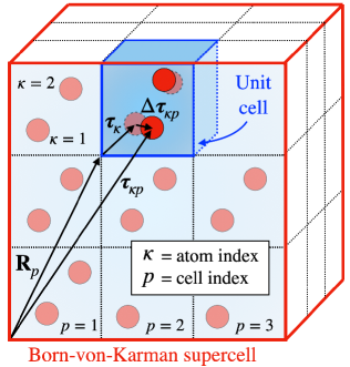
Figure 2: Schematic illustration of the Born-von-Karman supercell and of the notation adopted to denote the nuclear displacements from equilibrium.

The operator $\Delta\hat{\bm{\tau}}_{\kappa p}$ is a key quantity for the study of the lattice dynamics: its expectation value $\Delta{\bm{\tau}}_{\kappa p}(t)=\langle\Delta\hat{\bm{\tau}}_{\kappa p}(t)\rangle$ quantifies the displacement of a given nucleus from its equilibrium position at time $t$, and describes the coherent nuclear dynamics of the lattice. In the absence of a radiation filed, the eigenstates of a harmonic lattice are the eigenstates $|\chi_{{n}}\rangle$ of the Hamiltonian $\hat{H}_{\rm ph}$. They satisfy $\langle\chi_{n}|\hat{Q}_{{\bf q}\nu}|\chi_{{n}}\rangle=0$, thus, leading to vanishing displacements ${\bm{\tau}}_{\kappa p}(t)=0$. This is also the case for incoherent phonons which do not contribute to the average displacement of the nuclei. It is clear from the definition in Eq. (8) that a prerequisite for having non-vanishing displacements of the nuclear wave packets from equilibrium ($\Delta{\bm{\tau}}_{\kappa p}\neq 0$) is the expectation value of the operator $\hat{Q}_{{\bf q}\nu}$ to be finite, i.e., $Q_{{\bf q}\nu}=\langle\hat{Q}_{{\bf q}\nu}\rangle\neq 0$ [19]. Before proceeding to discuss how this condition is realized, we briefly outline the TDBE and its application to the description of the incoherent lattice dynamics.

III Incoherent phonons and the time-dependent Boltzmann equation

The TDBE is a well-established formalism to investigate the incoherent lattice dynamics and determine the change of phonon population $n_{{\bf q}\nu}$ for a vibrating lattice subject to external perturbations [32]. The influence of the electron-phonon coupling on the dynamics of phonons has been subject of several ab-initio studies based on the TDBE approach [30, 31, 59, 34]. In the following, we briefly discuss the application of the TDBE to the lattice dynamics of polar semiconductors interacting with a THz field. In this case, all bands are either filled or empty, and electron-phonon interactions are inconsequential for the dynamics. The TDBE reads:

$$\partial_{t}n_{{\bf q}\nu}=\Gamma^{\rm IR}_{{\bf q}\nu}(t)+\Gamma^{\rm pp}_{{\bf q}\nu}(t)\quad,$$ (9)

with $\partial_{t}=\partial/\partial t$. Here, $\Gamma^{\rm pp}_{{\bf q}\nu}$ is the scattering rate due to phonon-phonon interactions, which can be obtained by applying Fermi’s golden rule to the Hamiltonian $\hat{H}_{\rm pp}$ [32]. Alternatively, it can be expressed in the relaxation time approximation (RTA) as $\Gamma^{\rm pp}_{{\bf q}\nu}=-(n_{{\bf q}\nu}-n_{{\bf q}\nu}^{\rm eq})/\tau_{{\bf q}\nu}^{\rm pp}$ [30], where $n_{{\bf q}\nu}^{\rm eq}$ denotes the equilibrium Bose-Einstein distribution, and $\tau_{{\bf q}\nu}^{\rm pp}$ is the relaxation time due to phonon-phonon scattering [51]. $\Gamma^{\rm IR}_{{\bf q}\nu}$ is the collision integral due to IR absorption. We show in Appendix C that it takes the following integral form:

$$\Gamma^{\rm IR}_{{\bf q}\nu}(t)=e^{2}E_{0}^{2} \frac{|{\bf F}_{\nu}\cdot{\bm{\pi}}|^{2}}{\hbar\omega_{{\bf q}\nu}}\delta_{{\bf q}0}f(t)$$ (10)

$$\times\int_{-\infty}^{t}d\tau f(\tau)\cos[\omega_{{\bf q}\nu}(\tau-t)]\quad.$$

where ${\bf F}_{\nu}=\sum_{\kappa}{{{\bf Z}^{\text{*}}_{\kappa}}\cdot{\bf e}^{\kappa}_{0\nu}}\,M_{\kappa}^{-\frac{1}{2}}$ is the IR cross section of the phonon $\nu$, also called mode effective charge. Here, we express the electric field as ${\bf E}(t)=E_{0}{\bm{\pi}}f(t)$, where $E_{0}$ is the field intensity, $\bm{\pi}$ the light-polarization unitary vector, and $f(t)$ an adimensional time-envelop function.

Table 1: Computational parameters adopted in the investigation of the structural dynamics.

$\omega_{\rm IR}=\omega$	$\omega_{\rm R}$	$E_{0}$	${\bf Z}^{*}_{\kappa}$	$M_{\kappa}$	$|{\bf F}_{\nu}\cdot{\bm{\pi}}|$
6 THz	5 THz	100 kV cm-1	$\pm 6$	20 Da	0.05 $m_{e}^{-\frac{1}{2}}$

To exemplify the (incoherent) lattice dynamics resulting from the solution of Eq. (9), we illustrate in Fig. 3 the phonon distribution function $n_{{\bf q}\nu}$ for an IR-active mode with frequency $\omega_{\rm IR}=6$ THz coupled to a THz field with pulse profile $f(t)=\sin(\omega t)e^{-(t/2\tau)^{2}}$ and resonant frequency $\omega=\omega_{\rm IR}$. The variation of the pulse profile $f(t)$ for durations $\tau=0.1,0.3,$ and $1.0$ ps is shown in Figs. 4 (a-c). To solve Eq. (9) phonon-phonon scattering is accounted for in the RTA with relaxation times $\tau^{\rm pp}_{{\bf q}\nu}$ ranging between 1 and 10 ps and for the undamped limit ($\tau^{\rm pp}_{{\bf q}\nu}\rightarrow\infty$). We considered a pulse duration $\tau=2$ ps, and the field intensity is parametrized by setting $E_{0}=100$ kV cm^-1 and $|{\bf F}_{\nu}\cdot{\bm{\pi}}|=0.05$ $m_{e}^{-\frac{1}{2}}$. All parameters are summarized in Table LABEL:tab:param. The trend illustrated in Fig. 3 exhibits an initial rise, which reflects the increased phonon population due to IR absorption. This mechanism is analogous to the raise in quantum number of a driven quantum harmonic oscillator [Fig. 1 (a)]. On longer timescales, the decrease of the phonon number indicates the return to thermal equilibrium on timescales dictated by phonon-phonon relaxation time $\tau^{\rm pp}$. Different choices for the field intensity $E_{0}$ or IR cross section ${\bf F}_{\nu}$ do not alter this picture and lead to a simple rescaling of the $y$ axis in Fig. 3.

The dynamics of the phonon populations illustrated in Fig. 3 is a purely quantum effect of the lattice. In the classical picture, however, a similar trend can be deduced by exploiting the correspondence between the coherent vibrations and the mean-square displacements of the ions (Sec. VIII.1), and by employing phenomenological damping for the phonon-phonon interaction [42, 43].

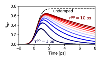
Figure 3: Change of phonon number for an IR-active phonon coupled to a THz field, obtained from the solution of Eq. (9). The computational parameters are summarized in Table LABEL:tab:param. Phonon-phonon collisions are treated in the relaxation time approximation by considering relaxation times $\tau^{\rm pp}$ ranging between 1 and 10 ps. The dynamics for the undamped limit ($\tau^{\rm pp}\rightarrow\infty$) is marked by a dashed line.

IV Equation of motion for the coherent lattice dynamics

We proceed below to derive the general EOM for the coherent dynamics of the lattice. More precisely, we are interested in determining the time dependence of the nuclear displacements $\Delta{\bm{\tau}}_{\kappa p}(t)$ for a system described by the Hamiltonian $\hat{H}=\hat{H}_{\rm ph}+\hat{H}_{\rm int}$, where $\hat{H}_{\rm int}$ denotes a generic perturbation. In short, we address this task by solving the Heisenberg EOM for the normal coordinate operator $\hat{Q}_{{\bf q}\nu}$ and deducing the nuclear displacements from $\Delta{\bm{\tau}}_{\kappa p}(t)=\langle\Delta\hat{\bm{\tau}}_{\kappa p}(t)\rangle$ via Eq. (8). Here and below, the Heisenberg picture is implied. To illustrate these steps, we begin by considering their application to an unperturbed harmonic lattice.

IV.1 Coherent dynamics of the harmonic lattice.

In an ideal harmonic lattice (i.e., for an Hamiltonian $\hat{H}=\hat{H}_{\rm ph}$) the Heisenberg EOM for the normal coordinate $\hat{Q}_{{\bf q}\nu}$, defined in Eq. (3), reads:

$$i\hbar{\partial_{t}\hat{Q}_{{\bf q}\nu}}=[\hat{Q}_{{\bf q}\nu},\hat{H}_{\rm ph}]\quad,$$ (11)

and similarly for $\hat{P}_{{\bf q}\nu}$. Making use of the commutators in Eqs. (43) and (44) we promptly obtain:

$$i\hbar{\partial_{t}\hat{Q}_{{\bf q}\nu}} =\hbar\omega_{{\bf q}\nu}\hat{P}_{{\bf q}\nu}\quad,$$ (12)

$$i\hbar{\partial_{t}\hat{P}_{{\bf q}\nu}} =\hbar\omega_{{\bf q}\nu}\hat{Q}_{{\bf q}\nu}\quad.$$ (13)

By taking once more the time derivative, these expressions can be combined to yield:

$${\partial^{2}_{t}{Q}_{{\bf q}\nu}}+\omega_{{\bf q}\nu}^{2}{Q}_{{\bf q}\nu}=0\quad,$$ (14)

where we introduced the notation ${Q}_{{\bf q}\nu}=\langle\hat{Q}_{{\bf q}\nu}\rangle$, and $\langle\dots\rangle$ denotes the expectation value taken with the initial state of the lattice. This is the EOM of a (classical) harmonic oscillator, which is solved by a linear combination of complex exponentials with suitable initial conditions. The time-dependent nuclear displacements $\Delta{\bm{\tau}}_{\kappa p}(t)$ can be promptly recovered through the transformation in Eq. (8). However, because $\langle\hat{Q}_{{\bf q}\nu}\rangle=0$ the displacements vanish identically, reflecting the absence of coherent atomic motion for an unperturbed harmonic lattice.

IV.2 Coherent dynamics in presence of interactions

We next proceed to derive the general EOM for a harmonic lattice in presence of an external perturbation $\hat{H}_{\rm int}$, i.e., we consider the Hamiltonian $\hat{H}=\hat{H}_{\rm ph}+\hat{H}_{\rm int}$. By following the procedure outlined in Sec. IV.1 we arrive at the Heisenberg EOM:

$$i\hbar{\partial_{t}\hat{Q}_{{\bf q}\nu}} =\hbar\omega_{{\bf q}\nu}\hat{P}_{{\bf q}\nu}\quad,$$ (15)

$$i\hbar{\partial_{t}\hat{P}_{{\bf q}\nu}} =\hbar\omega_{{\bf q}\nu}\hat{Q}_{{\bf q}\nu}+[\hat{P}_{{\bf q}\nu},\hat{H}_{\rm int}]\quad.$$ (16)

In Eq. (15), we made use of $[\hat{Q}_{{\bf q}\nu},\hat{H}_{\rm int}]=0$, which holds for the Hamiltonian introduced in Sec. II (see Appendix A). Equations (15) and (16) can be recast into a second-order differential equation for $Q_{{\bf q}\nu}$ by taking the time derivative of Eq. (15) and its expectation value. This procedure leads to the general EOM for the coherent lattice dynamics in presence of external perturbations:

$${\partial^{2}_{t}{Q}_{{\bf q}\nu}}+\omega_{{\bf q}\nu}^{2}Q_{{\bf q}\nu}=D_{{\bf q}\nu}(t)\quad,$$ (17)

where we introduced the abbreviation:

$$D_{{\bf q}\nu}(t)=-\hbar^{-1}\omega_{{\bf q}\nu}\langle[\hat{P}_{{\bf q}\nu},\hat{H}_{\rm int}]\rangle\quad.$$ (18)

Equation (17) assumes the familiar form of a driven harmonic oscillator EOM. The quantity $D_{{\bf q}\nu}(t)$ acts as a time-dependent driving term that can induced finite coherent phonon amplitudes ${Q}_{{\bf q}\nu}$ and a non-trivial dynamics of the lattice. The precise form of the driving force $D_{{\bf q}\nu}(t)$ and its time dependence depend on the nature of the interaction mechanism introduced by the Hamiltonian $\hat{H}_{\rm int}$. The driving term and its relation to the known mechanisms for the excitation of coherent phonons is discussed in more detail in Sec. V.

IV.3 Analytical solution for the coherent dynamics

If lattice anharmonicities are neglected ($\hat{H}_{\rm pp}=0$), the EOM can be solved analytically via the Green’s function method. The coherent phonon amplitudes can be recast in integral form as:

$${Q}_{{\bf q}\nu}(t)=\int_{-\infty}^{t}G_{{\bf q}\nu}(t,t^{\prime})D_{{\bf q}\nu}(t^{\prime})dt^{\prime}\quad.$$ (19)

Here, the Green’s function is given by $G_{{\bf q}\nu}(t,t^{\prime})={\sin[\omega_{{\bf q}\nu}(t-t^{\prime})]}/\omega_{{\bf q}\nu}$, and the time-dependence of the nuclear coordinates $\Delta{\bm{\tau}}_{\kappa p}(t)$ can be recovered recovered through substitution of Eq. (19) in Eq. (8). Equation (19) is the exact result for the coherent dynamics of an harmonic lattice. In this limit, the quantum and classical description coincide.

V Driving mechanisms for the excitations of coherent phonons

Below we discuss the form of the coherent phonon driving term in presence of electron-phonon coupling, external driving fields, and lattice anharmonicities. This procedure enables to derive the known mechanisms for the excitation of coherent phonon within a unified theoretical framework.

V.1 Infrared absorption

We begin by considering the IR driving mechanism, i.e., the direct excitation of IR-active modes through the interaction with an electro-magnetic field with frequency in the THz range. We evaluate Eq. (18) using the Hamiltonian $\hat{H}_{\rm IR}$ from Eq. (7) and making use of the commutator in Eq. (49). One promptly obtains:

$$D_{{\bf q}\nu}^{\rm IR}(t)=\delta_{{\bf q}0}{\bf C}_{\nu}\cdot{\bf E}(t)\quad.$$ (20)

Here, we defined ${\bf C}_{\nu}=eN_{p}^{\frac{1}{2}}(2\omega_{0\nu}/\hbar)^{\frac{1}{2}}{\bf F}_{\nu}$. The time dependence of the coherent phonon driving force $D_{{\bf q}\nu}^{\rm IR}$ is directly inherited from the electric field ${\bf E}(t)$. The quantity $D_{{\bf q}\nu}^{\rm IR}$ differs from zero only for zone-center ($\Gamma$ point) IR-active phonons. This follows directly from the dependence on the IR cross section ${\bf F}_{\nu}$ and the negligible momentum of THz photons as compared to the characteristic phonon momenta accessible in the Brillouin zone. Correspondingly, only IR-active phonons at $\Gamma$ may exhibit coherent motion in absence of lattice anharmonicities.

V.2 Electron-phonon coupling and the displacive excitation of coherent phonons

We proceed to consider the driving mechanism arising from the electron-phonon interaction, i.e., we consider the Hamiltonian $\hat{H}_{\rm eph}$. This mechanism coincides with the so-called displacive excitation of coherent phonons (DECP) [18, 19, 60, 61]. Combining Eqs. (6), (18), and (52), we arrive at:

$$D_{{\bf q}\nu}^{\rm eph}=-\frac{\omega_{{\bf q}\nu}}{\hbar N_{p}^{\frac{1}{2}}}\sum_{mn{\bf k}}g_{mn}^{\nu}({\bf k},-{\bf q})\hat{c}^{\dagger}_{m{\bf k}-{\bf q}}\hat{c}_{n{\bf k}}\quad.$$ (21)

To eliminate the dependence on the fermionic operators $\hat{c}^{\dagger}_{m{\bf k}-{\bf q}}$ and $\hat{c}_{n{\bf k}}$, we take the expectation values using an electronic state $|\Psi\rangle$. Neglecting non-diagonal terms of the density matrix, i.e., $\langle\Psi|c^{\dagger}_{m{\bf k}-{\bf q}}\hat{c}_{n{\bf k}}|\Psi\rangle\simeq f_{n{\bf k}}(t)\delta_{nm}\delta_{{\bf q},0}$ , one arrives at:

$$D_{{\bf q}\nu}^{\rm eph}(t)=-\frac{\omega_{{\bf q}\nu}}{\hbar N_{p}^{\frac{1}{2}}}\sum_{n{\bf k}}g_{nn}^{\nu}({\bf k},{\bf q})[f_{n{\bf k}}(t)-f_{n{\bf k}}(0)]\delta_{{\bf q},0}$$ (22)

where $f_{n{\bf k}}(t)$ denotes the electronic distribution function at time $t$. The equilibrium ($t=0$) value $f_{n{\bf k}}(0)$ has been subtracted because the lattice is assumed to be initially at equilibrium. Equation (22) can be easily generalized to account for non-diagonal elements of the density matrix [19]. A straightforward symmetry analysis of the electron-phonon coupling matrix elements $g_{nn}^{\nu}({\bf k},{\bf q}=0)$ reveals that the driving force $D_{{\bf q}\nu}^{\rm eph}(t)$ differs from zero only for modes of $A_{1g}$ symmetry at the $\Gamma$ point. However, coupling to lower symmetry modes or to phonons with finite wavevectors (${\bf q}\neq 0$) can arise if the density matrix exhibits non-vanishing non-diagonal elements. In short, $D_{{\bf q}\nu}^{\rm eph}(t)$ is a purely electronic driving mechanism that results from the change of the electronic occupation function $f_{n{\bf k}}(t)\neq f_{n{\bf k}}(0)$. An example of this case the excitation of electrons via a pump pulse. More generally, the DECP mechanism can persist even in absence of an external driving field. In particular, any physical process leading to a sufficiently rapid change (i.e., faster than the characteristic decoherence time) of the distribution function $f_{n{\bf k}}$ should also lead to the excitation of coherent phonons.

V.3 Inelastic stimulated Raman scattering

The direct excitation of coherent Raman-active phonons can arise via the inelastic stimulated Raman scattering (ISRS) mechanism. This process is the only mechanism for the direct excitation of coherent phonons in crystals where neither IR-active modes nor totally symmetric ($A_{1g}$) phonons are present (e.g., diamond or graphene), and therefore the IR and displacive mechanisms discussed in Secs. V.1 and V.2, respectively, are symmetry forbidden. The derivation of the driving force for ISRS is somewhat involved and it requires the applications of second-order time-dependent perturbation theory to the electron-phonon coupling driving force $D_{{\bf q}\nu}^{\rm eph}$ [Eq. (21)] to account for the effects of a off-resonance electric field [20, 23]. The resulting driving force $D_{{\bf q}\nu}^{\rm ISRS}$ depends quadratically on the field, and it can be expressed within the Placzek approximation as [62]:

$$D_{{\bf q}\nu}^{\rm ISRS}(t)=\Omega\sum_{\alpha\beta}\frac{\partial\chi_{\alpha\beta}}{\partial Q_{{\bf q}\nu}}E_{\alpha}(t)E_{\beta}(t)$$ (23)

where $\alpha$ and $\beta$ run over the Cartesian components and $\chi_{\alpha\beta}$ is the linear susceptibility. Earlier works suggested that the displacive mechanism and the corresponding driving force $D_{{\bf q}\nu}^{\rm eph}$ can be regarded as a special case of the ISRS mechanism [20].

V.4 Phonon-phonon scattering and ionic Raman scattering

Lattice anharmonicities yet provide an additional route for the coherent excitations that do not couple directly to light. An explicit expression for the coherent phonon driving force $D_{{\bf q}\nu}^{\rm 3pp}$ due to third-order anharmonicities is derived by combining Eqs. (5), (18), and (50), yielding:

$$D_{{\bf q}\nu}^{\rm 3pp}(t)=-\frac{\omega_{{\bf q}\nu}}{\hbar}\sum_{{\bf q}^{\prime}{\bf q}^{\prime\prime}}\sum_{\nu^{\prime}\nu^{\prime\prime}}\Psi^{(3)}_{\begin{subarray}{c}\nu\nu^{\prime}\nu^{\prime\prime}\\ -{\bf q}{\bf q}^{\prime}{\bf q}^{\prime\prime}\end{subarray}}\langle\hat{Q}_{{\bf q}^{\prime}\nu^{\prime}}\hat{Q}_{{\bf q}^{\prime\prime}\nu^{\prime\prime}}\rangle$$ (24)

where $\langle\cdots\rangle$ denote the expectation value with respect to the initial state of the lattice, and its evaluation requires an approximate treatment, as discussed in Secs. VII.1 and VII.2. Similarly, by considering fourth-order lattice anharmonicities (four-phonon scattering processes), we arrive at:

$$D_{{\bf q}\nu}^{\rm 4pp}(t)=-\frac{\omega_{{\bf q}\nu}}{3\hbar}\sum_{\begin{subarray}{c}{\bf q}^{\prime}{\bf q}^{\prime\prime}{\bf q}^{\prime\prime\prime}\\ \nu^{\prime}\nu^{\prime\prime}\nu^{\prime\prime\prime}\end{subarray}}\Psi^{(4)}_{\begin{subarray}{c}\nu\nu^{\prime}\nu^{\prime\prime}\nu^{\prime\prime\prime}\\ -{\bf q}{\bf q}^{\prime}{\bf q}^{\prime\prime}{\bf q}^{\prime\prime\prime}\end{subarray}}\langle\hat{Q}_{{\bf q}^{\prime}\nu^{\prime}}\hat{Q}_{{\bf q}^{\prime\prime}\nu^{\prime\prime}}\hat{Q}_{{\bf q}^{\prime\prime\prime}\nu^{\prime\prime\prime}}\rangle.$$ (25)

Lattice anharmonicities do not alter the coherent dynamics of the lattice at equilibrium. In presence of additional driving sources for the excitation of coherent phonons, as, e.g., the mechanism discussed in Secs. V.1-V.3, phonon-phonon scattering can lead to the indirect excitations of coherent phonons that are coupled by lattice anharmonicities. The mechanism of ionic Raman scattering (IRS), for example, is realized when a coherent IR phonon, photo-excited by IR absorption, drives the excitation of a coherent Raman mode via phonon-phonon scattering. IRS can be accounted from first principles by simultaneously accounting for the IR and the phonon-phonon scattering driving mechanisms $D_{{\bf q}\nu}^{\rm IR}$ and $D_{{\bf q}\nu}^{\rm 3pp}$, respectively, in the EOM of the lattice.

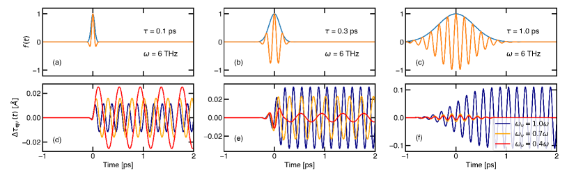
Figure 4: (a-c) Pulse profile $f(t)=\sin(\omega t)e^{-(2t/\tau)^{2}}$ (orange) for a frequency $\omega=$6 THz and a Gaussian envelop function (blue) with width $\tau=0.1$, 1, and 2 ps, respectively. (d-f) Time-dependence of the function $I_{\nu}(t)=\omega_{\nu}\int_{-\infty}^{t}{\sin[\omega_{\nu}(t-t^{\prime})]}f(t^{\prime})dt^{\prime}$ for phonon frequencies $\omega_{\nu}=1.0\,\omega$, $0.7\,\omega$, and $0.4\,\omega$.

VI Harmonic lattice in a THz field

In the following, we discuss the coherent dynamics of a harmonic crystal. For sake of conciseness, here and in the following we focus on the IR driving mechanism ($D_{{\bf q}\nu}^{\rm IR}$), although similar considerations can also be extended, with due adjustments, to the displacive and Raman driving terms ($D_{{\bf q}\nu}^{\rm eph}$ and $D_{{\bf q}\nu}^{\rm ISRS}$). In this case, the EOM for the lattice is promptly derived by combining the driving force $D_{{\bf q}\nu}^{\rm IR}(t)$ from Eq. (20), with the generalized EOM from Eq. (17):

$$\frac{\partial^{2}{Q}_{{\bf q}\nu}(t)}{\partial t^{2}}+\omega_{{\bf q}\nu}^{2}Q_{{\bf q}\nu}(t)=D_{{\bf q}\nu}^{\rm IR}(t)$$ (26)

Equation (26) can be solved numerically by ordinary finite-difference algorithms for second-order differential equations (e.g., Heun or Runge Kutta). The exact analytical solution of Eq. (26), however, can also be obtained by direct analytical solution, as outlined in Sec. IV.3, yielding:

$$\Delta{\bm{\tau}}_{\kappa p}(t)=2eE_{0}M_{\kappa}^{-\frac{1}{2}} \sum_{\nu}{\bf e}^{\kappa}_{0\nu}(\bm{\pi}\cdot{\bf F}_{\nu})I_{\nu}(t)\omega_{0\nu}^{-2}\quad.$$ (27)

where $I_{\nu}(t)$ is an adimensional function of time defined as:

$$I_{\nu}(t)=\omega_{0\nu}\int_{-\infty}^{t}{\sin[\omega_{0\nu}(t-t^{\prime})]}f(t^{\prime})dt^{\prime}\quad.$$

and it encodes the time dependence of the nuclear displacements along the $\nu$-th phonon mode. Equation (27) is the exact solution for the coherent dynamics of a harmonic lattice in an IR field and it generalizes the result obtained in Ref. [21] for a single phonon mode.

To illustrate the coherent dynamics triggered by a THz pulse, we report in Figs. 4 (d-f) the atomic displacement $\Delta{\bm{\tau}}_{\kappa p}$ evaluated from the numerical integration of Eq. (27) for the parameters listed in Table LABEL:tab:param. The field profile function $f(t)$ is illustrated in Figs. 4 (a-c) for a pulse duration of $\tau=0.1$, 1, and 2 ps and frequency $\omega=6$ THz. In addition to the resonance condition ($\omega=\omega_{0\nu}$), we further report numerical results for the off-resonance case ($\omega_{0\nu}=0.7\omega$ and $\omega_{0\nu}=0.4\omega$).

For impulsive perturbations [Figs. 4 (d)] – namely, for pulse durations shorter than the phonon period ($\tau<2\pi/\omega$) [Figs. 4 (a)]– coherent nuclear motion (i.e., $\Delta{\bm{\tau}}_{\kappa p}\neq 0$) arises for both resonant ($\omega=\omega_{0\nu}$) and non-resonant modes ($\omega\neq\omega_{0\nu}$). In other words, the resonance condition is not strictly enforced and also quasi-resonant modes can be driven by a THz field. For pulse durations comparable to or longer than the phonon period ($\tau>2\pi/\omega$) only resonant IR-active modes are excited [Figs. 4 (e-f)], whereas the dynamics of non-resonant modes is strongly suppressed and it leads to a strict enforcement of the resonance condition for long pulses.

For times longer than the pulse duration ($t>2\tau$) it is a good approximation to substitute $\int_{-\infty}^{t}$ with $\int^{\infty}_{-\infty}$ into Eq. (27), and a fully analytical solution can be found for the resonant case ($\omega=\omega_{0\nu}$):

$$\Delta{\bm{\tau}}_{\kappa p}(t) =\alpha\cos(\omega t)eE_{0}M_{\kappa}^{-\frac{1}{2}}\sum_{\nu}{\bf e}^{\kappa}_{0\nu}(\bm{\pi}\cdot{\bf F}_{\nu})$$ (28)

where $\alpha={\tau\sqrt{\pi}}(1-e^{-\frac{\omega^{2}\tau^{2}}{4}})$, and the sum extends over all resonant IR-active modes. This expression provide a simple tool to estimate the maximum displacements induced by a THz field in a harmonic lattice. In particular, in presence of a single resonant mode, the maximum displacement of the nuclei induced by the field simply reduces to $\Delta{\bm{\tau}}_{\kappa p}^{\rm max}=c_{0}{\bf e}^{\kappa}_{0\nu}$ with $c_{0}=\alpha eE_{0}M_{\kappa}^{-\frac{1}{2}}(\bm{\pi}\cdot{\bf F}_{\nu})$.

VII Coherent dynamics of the anharmonic lattice

We thus proceed to investigate the effect of anharmonicities on coherent lattice dynamics in presence of a THz driving field. Replacing Eqs. (20), (24), and (25) into Eq. (17), we obtain the general EOM for an THz-driven anharmonic lattice:

$$\partial_{t}^{2} Q_{{\bf q}\nu}+\omega_{{\bf q}\nu}^{2}Q_{{\bf q}\nu}=\delta_{{\bf q}0}{\bf C}_{\nu}\cdot{\bf E}(t)$$ (29)

$$-\frac{\omega_{{\bf q}\nu}}{\hbar}\sum_{{\bf q}^{\prime}{\bf q}^{\prime\prime}}\sum_{\nu^{\prime}\nu^{\prime\prime}}\Psi^{(3)}_{\begin{subarray}{c}\nu\nu^{\prime}\nu^{\prime\prime}\\ -{\bf q}{\bf q}^{\prime}{\bf q}^{\prime\prime}\end{subarray}}\langle\hat{Q}_{{\bf q}^{\prime}\nu^{\prime}}\hat{Q}_{{\bf q}^{\prime\prime}\nu^{\prime\prime}}\rangle$$

$$-\frac{\omega_{{\bf q}\nu}}{3\hbar}\sum_{{\bf q}^{\prime}{\bf q}^{\prime\prime}{\bf q}^{\prime\prime\prime}}\sum_{\nu^{\prime}\nu^{\prime\prime}\nu^{\prime\prime\prime}}\Psi^{(4)}_{\begin{subarray}{c}\nu\nu^{\prime}\nu^{\prime\prime}\nu^{\prime\prime\prime}\\ -{\bf q}{\bf q}^{\prime}{\bf q}^{\prime\prime}{\bf q}^{\prime\prime\prime}\end{subarray}}\langle\hat{Q}_{{\bf q}^{\prime}\nu^{\prime}}\hat{Q}_{{\bf q}^{\prime\prime}\nu^{\prime\prime}}\hat{Q}_{{\bf q}^{\prime\prime\prime}\nu^{\prime\prime\prime}}\rangle$$

This expression defines a coupled set of $N_{p}\times N_{\rm ph}$ differential equations, with $N_{\rm ph}$ being the number of phonons branches, respectively. While analytical solution is not possible, approximations can be introduced to solve it numerically. This can accomplished by: (i) neglecting quantum effects (Sec. VII.1); (ii) retaining only the lowest order in the interaction (Sec. VII.2).

VII.1 Classical approximation and non-linear phononics models

A classical approximation to Eq. (29) can be deduced by neglecting quantum correlations and thereby writing $\langle\hat{Q}_{{\bf q}^{\prime}\nu^{\prime}}\hat{Q}_{{\bf q}^{\prime\prime}\nu^{\prime\prime}}\rangle\simeq\langle\hat{Q}_{{\bf q}^{\prime}\nu^{\prime}}\rangle\langle\hat{Q}_{{\bf q}^{\prime\prime}\nu^{\prime\prime}}\rangle=Q_{{\bf q}^{\prime}\nu^{\prime}}Q_{{\bf q}^{\prime\prime}\nu^{\prime\prime}}$ and similarly for fourth-order anharmonicities. This approximation is equivalent to treat nuclei as classical particles, and it is the most widely employed in the description of coherent lattice dynamics. Correspondingly, one arrives at the classical EOM for the dynamics of an anharmonic lattice in a THz field:

$$\partial_{t}^{2} Q_{{\bf q}\nu}+\omega_{{\bf q}\nu}^{2}Q_{{\bf q}\nu}=\delta_{{\bf q}0}{\bf C}_{\nu}\cdot{\bf E}(t)$$ (30)

$$-\frac{\omega_{{\bf q}\nu}}{\hbar}\sum_{\nu^{\prime}\nu^{\prime\prime}}\sum_{{{\bf q}^{\prime}{\bf q}^{\prime\prime}}}\Psi^{(3)}_{\begin{subarray}{c}{\nu\nu^{\prime}\nu^{\prime\prime}}\\ {{\bf q}{\bf q}^{\prime}{\bf q}^{\prime\prime}}\end{subarray}}Q_{{\bf q}^{\prime}\nu^{\prime}}Q_{{\bf q}^{\prime\prime}\nu^{\prime\prime}}$$

$$-\frac{\omega_{{\bf q}\nu}}{3\hbar}\sum_{{\bf q}^{\prime}{\bf q}^{\prime\prime}{\bf q}^{\prime\prime\prime}}\sum_{\nu^{\prime}\nu^{\prime\prime}\nu^{\prime\prime\prime}}\Psi^{(4)}_{\begin{subarray}{c}\nu\nu^{\prime}\nu^{\prime\prime}\nu^{\prime\prime\prime}\\ {\bf q}{\bf q}^{\prime}{\bf q}^{\prime\prime}{\bf q}^{\prime\prime\prime}\end{subarray}}Q_{{\bf q}^{\prime}\nu^{\prime}}Q_{{\bf q}^{\prime\prime}\nu^{\prime\prime}}Q_{{\bf q}^{\prime\prime\prime}\nu^{\prime\prime\prime}}$$

Simplified versions of Eq. (30) are widely employed in non-linear phononics to model the coherent structural dynamics driven by the absorption of THz fields [36, 40, 4, 43]. Non-linear phononics models typically rely on the following approximations: anharmonic coupling is restricted to two or few phonons; quantum nuclear effects are neglected; only zone-center ($\Gamma$ point) phonons are considered. Some of these limitations can be easily lifted by noticing that Eq. (30) is nothing else than the normal-coordinate representation of the ordinary classical EOM of the lattice:

$$M_{\kappa}\Delta{\ddot{\bm{\tau}}}_{\kappa p}=\mathbfcal{F}_{\kappa}(t)+\frac{\partial}{\partial\Delta{{\bm{\tau}}}_{\kappa p}}U(\{\Delta{{\bm{\tau}}}_{\kappa p}\})$$ (31)

where $\mathbfcal{F}_{\kappa}(t)=e{\bf E}(t)\cdot{\bf Z}_{\kappa}^{*}$ is the force acting on $\kappa$-th nucleus due to the field ${\bf E}(t)$, and $U(\{\Delta{{\bm{\tau}}}_{\kappa p}\})$ is the potential energy surface expanded up to fourth order in the nuclear displacements. As long as lattice anharmonicities are included at the same order, Eqs. (30) and (31) are completely equivalent formulations of the lattice dynamics in normal and Cartesian coordinates, respectively. Additionally, one can reversibly change representation from normal to Cartesian coordinates (and viceversa) via Eq. (8) and the inverse transformation:

$$Q_{{\bf q}\nu}=\sum_{\kappa p}\left(\frac{M_{\kappa}}{M_{0}N_{p}}\right)^{\frac{1}{2}}e^{-i{{\bf q}}\cdot{\bf R}_{p}}l_{{\bf q}\nu}^{-1}[{\bf e}^{\kappa}_{{\bf q}\nu}]^{*}\cdot\Delta{{\bm{\tau}}}_{\kappa p}\quad.$$ (32)

Equation (31) can be efficiently solved via AIMD by directly computing the gradients of the potential-energy surface $U$ from Kohn-Sham density-functional theory for a given displaced nuclear configuration.

VII.2 Quantum nuclear effects

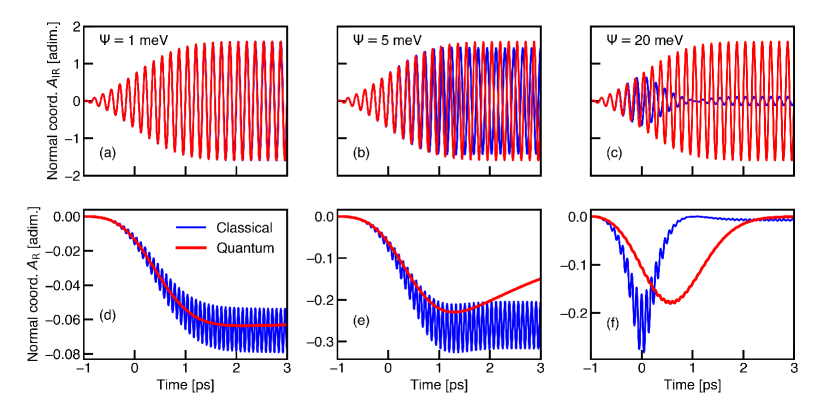
Figure 5: Dynamics of the normal coordinate $Q_{\rm IR}$ of the IR-active mode for third-order anharmonic coupling constant $\Psi=1$, 5, and 20 meV [(a), (b), and (c), respectively], as obtained from the time-propagation of the classical EOM (blue, Eqs. (36) and (37)) and from the quantum EOM (red, Eqs. (38) and (39)) of the two-phonon model. (d-f) Dynamics of the normal coordinate $Q_{\rm R}$ of the Raman-active mode corresponding to the same anharmonic coupling $\Psi$ as in (a-c). The result of the classical (quantum) EOM is reported in blue (red).

Having illustrated in Sec. VII.1 the classical approximation to the lattice EOM, we proceed here to discuss the inclusion of quantum nuclear effects on the dynamics. To address this task, we make use of the following identity:

$$\langle\hat{Q}_{{\bf q}\nu}(t)\hat{Q}_{{\bf q}^{\prime}\nu^{\prime}}(t)\rangle=[2n_{{\bf q}\nu}(t)+1]\delta_{-{\bf q}{\bf q}^{\prime}}\delta_{\nu\nu^{\prime}}\quad.$$ (33)

Here $n_{{\bf q}\nu}(t)$ is the (incoherent) population of the phonon ${{\bf q}\nu}$ at time $t$ which can be directly obtained from the solution of the TDBE (Sec. III). Substitution of Eq. (33) into Eq. (29) yields the quantum EOM for an anharmonic lattice in presence of a THz field:

$$\partial_{t}^{2}Q_{{\bf q}\nu}+ \omega_{{\bf q}\nu}^{2}Q_{{\bf q}\nu}=\delta_{{\bf q}0}{\bf C}_{\nu}\cdot{\bf E}(t)$$ (34)

$$-\frac{\omega_{{\bf q}\nu}}{\hbar}\sum_{{\bf q}^{\prime}\nu^{\prime}}\Psi^{(3)}_{\begin{subarray}{c}\nu\nu^{\prime}\nu^{\prime}\\ -{\bf q}{\bf q}^{\prime}-{\bf q}^{\prime}\end{subarray}}[2n_{{\bf q}^{\prime}\nu^{\prime}}(t)+1]\quad.$$

From the inspection of the phonon-phonon coupling matrix element $\Psi^{(3)}$, the symmetry requirements for which the anharmonic corrections to Eq.(34) become important can be easily deduced by elementary group-theoretical considerations [63, 64]. Namely, a prerequisite for the matrix elements $\Psi^{(3)}$ to be finite is that the direct product of the irreducible representations of the phonons involved in the scattering process contains the totally-symmetric representation of the group $\Gamma_{1}$, that is, $\Gamma_{{\bf q}\nu}\otimes\Gamma_{{\bf q}^{\prime}\nu^{\prime}}\otimes\Gamma_{-{\bf q}^{\prime}\nu^{\prime}}\supseteq\Gamma_{1}$. In particular, because the phonons ${\bf q}^{\prime}\nu^{\prime}$ and $-{\bf q}^{\prime}\nu^{\prime}$ belong to the same irreducible representation, the direct product $\Gamma_{{\bf q}^{\prime}\nu^{\prime}}\otimes\Gamma_{-{\bf q}^{\prime}\nu^{\prime}}$ equals the totally symmetric representation $\Gamma_{1}$. Therefore, the matrix elements $\Psi^{(3)}$ differs from zero only if $\Gamma_{{\bf q}\nu}$ contains (or is equal to) $\Gamma_{1}$. This symmetry requirement is violated for IR-active phonons or more generally for phonons involving low-symmetry motion of the atoms. The EOM for the normal coordinates corresponding to these modes reduces to Eq. (26) and it is unaffected by (third-order) lattice anharmonicities. The symmetry condition is satisfied by fully symmetric Raman-active modes ($A_{1g}$) for which the anharmonic term in the Eq. (34) remains finite. More generally, other combinations of phonon symmetries allow for non-vanishing phonon-phonon coupling matrix elements, and can therefore be driven by the mechanism in Eq. (34). In this case, the EOM resembles the problem of the forced harmonic oscillator which – for slow variations for the phonon occupation $n_{{\bf q}^{\prime}\nu^{\prime}}(t)$ of the driven mode – can be approximately solved to yield an explicit expression for the time-dependent normal coordinate $Q^{\rm R}_{\nu}$ of the Raman mode:

$$Q^{\rm R}_{\nu}(t)=-(\hbar\omega_{\nu})^{-1}\sum_{{\bf q}^{\prime}\nu^{\prime}}\Psi^{(3)}_{\begin{subarray}{c}\nu\nu^{\prime}\nu^{\prime}\\ 0{\bf q}^{\prime}-{\bf q}^{\prime}\end{subarray}}[2n_{{\bf q}^{\prime}\nu^{\prime}}(t)+1]\quad.$$ (35)

The expression for the nuclear displacement $\Delta{\bm{\tau}}_{\kappa p}$ is recovered by combining Eqs. (8) and (35). This mechanism is the quantum counterpart of ionic Raman scattering and nonlinear phonon rectification, typically described within the classical harmonic oscillator model. Several considerations can be immediately deduced from Eq. (35), which reveal the differences between a quantum and classical description of the coherent lattice dynamics: (i) The displacement of the lattice along totally symmetric modes (or along other modes complying with the symmetry requirements outlined above) results from the enhancement of the phonon population $n_{{\bf q}\nu}$, rather than from the coherent phonon amplitude. This indicates that ionic Raman scattering is an inherently incoherent process. In other words, it results from the enhanced population of strongly-coupled modes (as, e.g., driven IR-active modes), but it does not necessarily requires the excitation of coherent phonons. (ii) The displacement of the lattice along totally-symmetric Raman modes contains a zero-point motion (ZPM) component $Q^{\rm ZPM}_{\nu}=-(\hbar\omega_{\nu})^{-1}\sum_{{\bf q}^{\prime}\nu^{\prime}}\Psi^{(3)}_{\begin{subarray}{c}\nu\nu^{\prime}\nu^{\prime}\\ 0{\bf q}^{\prime}{\bf q}^{\prime}\end{subarray}}$, which should be present even at thermal equilibrium and zero temperature. $Q^{\rm ZPM}_{\nu}$ quantifies the displacement of the nuclear wave packets from thermal equilibrium (i.e., from $\Delta{\bm{\tau}}_{\kappa p}=0$) due to anharmonicity. (iii) The time scales for light-induced structural displacements due to ionic Raman scattering are limited by he characteristic anharmonic lifetime of the driven IR-active mode. In crystalline solids, three-phonon scattering processes are the leading contribution to the mode lifetime and they are accounted for by the collision integral $\Gamma^{\rm pp}(t)$ within the framework of the Boltzmann equation (Eq. (9)).

VIII Two phonon model

To illustrate the key differences between a classical and quantum formulation of the coherent dynamics, we solved the classical [Eq. (34)] and quantum EOM [Eq. (30)] for a model system consisting of two coupled phonon modes. In particular, we consider an IR-active mode with frequency $\omega_{\rm IR}=6$ THz, an electromagnetic field with frequency $\omega=\omega_{\rm IR}$, and a fully-symmetric Raman-active mode with frequency $\omega_{\rm R}=0.8\omega_{\rm IR}$ coupled to the IR mode via third-order anharmonicities. Fourth-order anharmonicities are neglected in the following. Symmetry requires the coupling matrix elements to satisfy $\Psi_{\rm IR,IR,R}^{(3)}=\Psi^{(3)}_{\rm IR,R,IR}=\Psi^{(3)}_{\rm R,IR,IR}\equiv\Psi\neq 0$ and $\Psi_{\rm IR,R,R}^{(3)}=\Psi^{(3)}_{\rm R,IR,R}=\Psi^{(3)}_{\rm R,R,IR}=0$. Correspondingly, the classical EOM [Eq. (30)] for the normal coordinates of the IR- and Raman-active modes, $Q_{\rm IR}$ and $Q_{\rm R}$, reduces to:

$$\partial_{t}^{2}Q_{\rm IR}+\omega_{\rm IR}^{2}Q_{\rm IR} ={C}_{\rm IR}{E_{0}}(t)+g_{\rm IR}Q_{\rm R}Q_{\rm IR}$$ (36)

$$\partial_{t}^{2}Q_{\rm R}+\omega_{\rm R}^{2}Q_{\rm R} =g_{\rm R}Q_{\rm IR}^{2}\quad,$$ (37)

where $C_{\rm IR}$ is defined as in Eq. (26), and we introduced the effective anharmonic coupling constants $g_{\rm IR}=-2\hbar^{-1}\omega_{\rm IR}\Psi$ and $g_{\rm R}=-\hbar^{-1}\omega_{\rm R}\Psi$. More generally, the effective coupling constant $g$ is related to the phonon-phonon coupling matrix element via $g_{\nu\nu^{\prime}\nu^{\prime\prime}}=-\hbar^{-1}\omega_{\nu}\Psi_{\nu\nu^{\prime}\nu^{\prime\prime}}^{(3)}$. From similar considerations, we deduce from Eq. (34) the quantum EOM for the two-phonon model:

$$\partial_{t}^{2}Q_{\rm IR}+\omega_{\rm IR}^{2}Q_{\rm IR} ={C}_{\rm IR}{E_{0}}f(t)$$ (38)

$$\partial_{t}^{2}Q_{\rm R}+\omega_{\rm R}^{2}Q_{\rm R} =2g_{\rm R}n_{\rm IR}(t)$$ (39)

where $n_{\rm IR}$ is the time-dependent phonon population of the IR-active mode, which is obtained from the solution of the time-dependent Boltzmann equation Eq. (9). Here, we omitted the zero-point motion contribution $Q^{\rm ZPM}_{\nu}$ to the normal coordinate, as its effect is limited to a renormalization of the equilibrium crystal structure. Additionally, we note that the back-coupling of Raman mode $Q_{\rm R}$ on the IR mode $Q_{\rm IR}$ is absent in the quantum approach, as a consequence of the identity in Eq. (33). We solved numerically the classical EOM [Eqs. (36) and (37)] by time-stepping the time derivative via the Heun’s finite-difference algorithm, whereas the quantum EOM, Eqs. (38) and (39), have been solved simultaneously to Eq. (9) to account for the increased population of IR phonons due to IR absorption. The field intensity and IR cross section are evaluated considering realistic parameter values [see Table LABEL:tab:param], and we considered a pulse duration of $1$ ps.

In Fig. 5 (a-c), we compare the dynamics of the normal coordinate $Q_{\rm IR}$ of the IR-active mode obtained from the solution of the classical (blue) and quantum (red) EOM, for increasing anharmonic coupling constant $\Psi$. For low anharmonic coupling (Fig. 5 (a)), the classical and quantum dynamics of the IR mode coincide, and they follow a trend similar to the one illustrated in Fig. 4 for an ideal harmonic lattice. The dynamics of the IR mode as obtained from the quantum EOM is unaffected by the value of $\Psi$, whereas the result of the classical EOM exhibits a dependence on the anharmonic coupling constant, which leads to an increasing discrepancy with the quantum EOM in the strong coupling regime (Figs. 5 (b) and (c)). This effect can be attributed to the influence that the Raman mode exerts on the IR-mode dynamics (second term in the right-hand side of Eq. (36)), which is suppressed in the quantum EOM (right-hand side of Eq. (38)).

The dynamics of the normal coordinate $Q_{\rm R}$ of the Raman mode is illustrated in Figs. 5 (d-f) for increasing anharmonic coupling constant $\Psi$. On short time scales, the normal coordinate $Q_{\rm R}$ obtained from the quantum EOM exhibits a progressive shift away from the initial value $Q_{\rm R}=0$, whereas on longer time scales, $Q_{\rm R}$ returns to zero on timescales that are dictated by the phonon-phonon coupling strength. This trend can be ascribed to the changes in phonon occupation of the IR-active mode, illustrated in Fig. 3, whose rise and decay stems from IR absorption and phonon-phonon scattering, respectively. This behaviour is the quantum counterpart of the ionic Raman scattering process [36, 37]. While on the hand the results of the classical (blue) and quantum EOM (red) follow qualitatively similar trends, the classical results leads to periodic oscillations of the normal coordinates. This behaviour is further discussed in Sec. VIII.1. The agreement between quantum and classical picture can further be ameliorated through the inclusion of a phenomenological damping term to account for the decoherence of the coherent phonon amplitude. Interestingly, the shift of the normal coordinate $Q_{\rm R}$ [Eq. (35)] depends exclusively on (i) the phonon-phonon coupling matrix elements $\Psi$ and (ii) the instantaneous population of all phonons. These points suggest that it may be possible to systematically assess and quantify light-induced structural distortions via calculations of the third-order force constants of the IR activity alone, i.e., without the need for an explicit solution of the EOM of the lattice.

VIII.1 Classical vs quantum nuclear dynamics

To illustrate to which extent the coherent motion of the nuclei relates to the incoherent dynamics of the lattice one can note that the phonon occupations $n_{\nu}$ of zone-center phonons can be expressed as:

$$\langle\hat{Q}_{\nu}\hat{Q}_{\nu}\rangle=2n_{\nu}+1\quad.$$ (40)

Neglecting zero-point motion and quantum nuclear effects ($\langle\hat{Q}_{\nu}\hat{Q}_{\nu}\rangle\simeq Q_{\nu}^{2}$), an approximate relation between phonon number and normal coordinate can be deduced: $Q_{\nu}^{2}\simeq 2n_{\nu}$. In absence of decoherence or lattice anharmonicities, the amplitude of THz-driven coherent nuclear motion can thus be approximately related to the number of IR-active modes excited in the system.

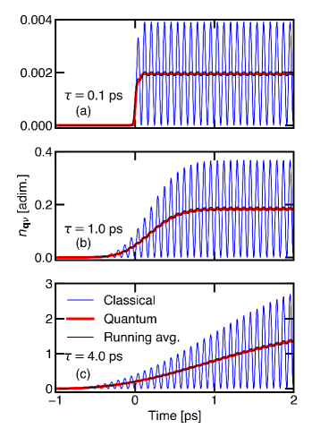
Figure 6: Comparison between the phonon number $n_{\nu}$ (red), obtained from the solution of the TDBE [Eq. (9)] and from the classical approximation $n_{\nu}\simeq Q_{\nu}^{2}/2$ for a pulse duration $\tau=0.1$ (a), 1 (b), and 10 ps (c). For comparison, the running average of classical approximation is included (black line) and it reveals excellent agreement with the quantum results.

We illustrate this point by comparing in Fig. 6 the phonon occupation $n_{\nu}$ and corresponding classical approximation $Q_{\nu}^{2}/2$ for an IR active phonon resonant to a THz field obtained from the numerical solution of Eqs. (26) and (9). We consider a frequency $\omega_{\rm IR}=6$ THz, and pulse durations $\tau=0.1$, 1, and 10 ps [(a), (b), and (c), respectively]. The monotonic increase of the phonon occupations (red) reflects phonon emission processes resulting from the IR absorption in absence of dissipation, decoherence, and anharmonicities. The classical approximation to the phonon number, conversely, exhibits an oscillatory character, where the oscillation center coincides with the exact (quantum) phonon number. In this case, the oscillations reflects the conversion of kinetic and potentials energy (and vice versa). This artifact can be eliminated by considering the running average of the classical oscillation amplitudes (black line in Fig. 6), which agrees well with the phonon populations derived from the solution of the TDBE.

IX Conclusions

We discussed the coherent structural dynamics of solids subject to the interaction with strong fields and its theoretical foundation. Our approach is based on the solution of the Heisenberg equation for the nuclear displacement operator, and it enables to derive a generalized EOM for coherent dynamics of the crystalline lattice in presence of several interaction mechanisms. The lattice EOM can be solved exactly in some limiting case (e.g., for an harmonic lattice interacting with a field), and it provides a way to systematically include quantum nuclear effects in presence of anharmonicities. Additionally, all known mechanisms for the excitation of coherent phonons can be accounted for within a unified theoretical framework. Classical approximations to the coherent lattice dynamics (non-linear phononics model) can be immediately deduced by neglecting the quantum character of the nuclei.

These findings shed light on the origin of light-induced structural control in THz-driven crystals. In particular, the structural distortion of the lattice along fully-symmetric Raman active modes (ionic Raman scattering) emerges as an incoherent process that results from the enhanced population of anharmonically-coupled IR-active modes. The incoherent nature of the ionic Raman scattering mechanism suggests that indirect control of the non-equilibrium phonon population can provide a new route to engineer transient structural changes in solids. This picture corroborates and generalizes the finding of earlier studies, whereby coherent structural dynamics was predicted on the basis of the classical EOM. Our findings further predict a zero-point motion displacements of the nuclear wave packets along Raman-active modes which is a fully quantum effect. This effect is not captured by classical approximations, and it should occur even in absence of external perturbations. Several of the analytical results deduced in this work are amenable for fully ab-initio simulations. Overall, our findings establish a rigorous theoretical foundation for the light-driven coherent lattice dynamics and for the widely-employed semi-classical models in the field of nonlinear phononics. Our approach is further suitable to account for novel phenomena that can trigger the coherent dynamics of the lattice, such as, e.g., coherent phonon excitation due spin-phonon coupling in light-driven ferro-magnets.

Appendix A Commutators relations for $\hat{Q}_{{\bf q}\nu}$ and $\hat{P}_{{\bf q}\nu}$

In this appendix, we summarize the commutation relations for the operators $\hat{Q}_{{\bf q}\nu}=\hat{a}_{{\bf q}\nu}+\hat{a}^{\dagger}_{-{\bf q}\nu}$ and $\hat{P}_{{\bf q}\nu}=\hat{a}_{{\bf q}\nu}-\hat{a}^{\dagger}_{-{\bf q}\nu}$, which are required for the derivation of the EOM of the lattice:

$$[\hat{Q}_{{\bf q}\nu},\hat{Q}_{{\bf q}^{\prime}\nu^{\prime}}] =[\hat{P}_{{\bf q}\nu},\hat{P}_{{\bf q}^{\prime}\nu^{\prime}}]=0\quad,$$ (41)

$$[\hat{P}_{{\bf q}\nu},\hat{Q}_{{\bf q}^{\prime}\nu^{\prime}}] =2\delta_{-{\bf q}{\bf q}^{\prime}}\delta_{\nu\nu^{\prime}}\quad.$$ (42)

Equations (41) and (42) follow directly from the commutation relations for the bosonic operators $[\hat{a}_{{\bf q}\nu},\hat{a}_{{\bf q}^{\prime}\nu^{\prime}}^{\dagger}]=\delta_{{\bf q}{\bf q}^{\prime}}\delta_{\nu\nu^{\prime}}$ and $[\hat{a}_{{\bf q}\nu},\hat{a}_{{\bf q}^{\prime}\nu^{\prime}}]=[\hat{a}_{{\bf q}\nu}^{\dagger},\hat{a}^{\dagger}_{{\bf q}^{\prime}\nu^{\prime}}]=0$. The commutators with the Hamiltonians specified in Eqs. (2), (5), (6), and (7) can be easily derived by application of Eqs. (41) and (42):

$$[\hat{Q}_{{\bf q}\nu},\hat{H}_{\rm ph}] =\hbar\omega_{{\bf q}\nu}\hat{P}_{{\bf q}\nu}$$ (43)

$$[\hat{P}_{{\bf q}\nu},\hat{H}_{\rm ph}] =\hbar\omega_{{\bf q}\nu}\hat{Q}_{{\bf q}\nu}$$ (44)

$$[\hat{Q}_{{\bf q}\nu},\hat{H}_{\rm IR}] =0$$ (45)

$$[\hat{Q}_{{\bf q}\nu},\hat{H}^{(3)}_{\rm pp}] =0$$ (46)

$$[\hat{Q}_{{\bf q}\nu},\hat{H}^{(4)}_{\rm pp}] =0$$ (47)

$$[\hat{Q}_{{\bf q}\nu},\hat{H}_{\rm eph}] =0$$ (48)

$$[\hat{P}_{{\bf q}\nu},\hat{H}_{\rm IR}] =-2e\delta_{{\bf q}0}\left(M_{0}N_{p}\right)^{\frac{1}{2}}l_{{\bf q}\nu}{\bf E}(t)\cdot{\bf F}_{\nu}$$ (49)

$$[\hat{P}_{{\bf q}\nu},\hat{H}_{\rm pp}^{(3)}] =\sum_{{\bf q}^{\prime}{\bf q}^{\prime\prime}}\sum_{\nu^{\prime}\nu^{\prime\prime}}\Psi^{(3)}_{\begin{subarray}{c}\nu\nu^{\prime}\nu^{\prime\prime}\\ -{\bf q}{\bf q}^{\prime}{\bf q}^{\prime\prime}\end{subarray}}\hat{Q}_{{\bf q}^{\prime}\nu^{\prime}}\hat{Q}_{{\bf q}^{\prime\prime}\nu^{\prime\prime}}$$ (50)

$$[\hat{P}_{{\bf q}\nu},\hat{H}_{\rm pp}^{(4)}] =\frac{1}{3}\sum_{\begin{subarray}{c}{{\bf q}^{\prime}{\bf q}^{\prime\prime}{\bf q}^{\prime\prime\prime}}\\ {\nu^{\prime}\nu^{\prime\prime}\nu^{\prime\prime\prime}}\end{subarray}}\Psi^{(4)}_{\begin{subarray}{c}\nu\nu^{\prime}\nu^{\prime\prime}\nu^{\prime\prime\prime}\\ -{\bf q}{\bf q}^{\prime}{\bf q}^{\prime\prime}{\bf q}^{\prime\prime\prime}\end{subarray}}\hat{Q}_{{\bf q}^{\prime}\nu^{\prime}}\hat{Q}_{{\bf q}^{\prime\prime}\nu^{\prime\prime}}\hat{Q}_{{\bf q}^{\prime\prime\prime}\nu^{\prime\prime\prime}}$$ (51)

$$[\hat{P}_{{\bf q}\nu},\hat{H}_{\rm eph}] =N_{p}^{-\frac{1}{2}}\sum_{mn{\bf k}}g_{mn}^{\nu}({\bf k},-{\bf q})\hat{c}^{\dagger}_{m{\bf k}-{\bf q}}\hat{c}_{n{\bf k}}$$ (52)

In Eq. (49), the vector ${\bf F}_{\nu}=\sum_{\kappa}{{{\bf Z}^{\text{*}}_{\kappa}}\cdot{\bf e}^{\kappa}_{\nu}}\,M_{\kappa}^{-\frac{1}{2}}$ is the IR cross section of the phonon $\nu$ with ${{\bf q}=0}$, which differs from zero only for IR-active phonons. Equation (50) has been obtained by taking advantage of the symmetry properties of the third- and fourth-order phonon-phonon coupling matrix elements which are inherited by the corresponding force constant matrices [65].

Appendix B Effective Hamiltonian due to a THz field

In this appendix, we report a derivation of the Hamiltonian term arising from the interaction with THz fields. In presence of an electromagnetic field, the kinetic energy of electrons and nuclei gets modified according to Peierl’s substitution:

$$\hat{H}_{\rm IR}=\sum_{i}\frac{e}{m_{e}}{\bf A}\cdot\hat{\bf p}_{i}-\sum_{\kappa p}\frac{Z_{\kappa}e}{M_{\kappa}}{\bf A}\cdot\hat{\bf P}_{\kappa p}$$ (53)

where $Z_{\kappa}$ is the charge of the $\kappa$-th nucleus, ${\bf A}$ is the vector potential, and $\hat{\bf P}_{\kappa p}$ is the nuclear momentum. Making use of the relations: $\langle\Phi_{f}|\hat{\bf P}_{\kappa p}|\Phi_{i}\rangle=iM_{\kappa}\omega\langle\Phi_{f}|\hat{\bm{\tau}}_{\kappa p}|\Phi_{i}\rangle$, and analogously for $\hat{\bf p}_{i}$, the effective Hamiltonian due to coupling with the field can be expressed as:

$$\hat{H}_{\rm IR}=e\sum_{i}{\bf E}\cdot\hat{{\bf r}}_{i}-e\sum_{\kappa p}{Z_{\kappa}}{\bf E}\cdot\Delta\hat{\bm{\tau}}_{\kappa p}=\hat{H}_{\rm IR}^{\rm(e)}+\hat{H}_{\rm IR}^{\rm(n)}$$ (54)

where ${\bf E}=-\partial_{t}{\bf A}$. Below we are interested in polar semiconductors with a band gap larger than the energy of incident phonons $\hbar\omega$. We can therefore restrict ourselves to consider matrix elements of the Hamiltonian $\hat{H}_{\rm IR}$ involving Born-Oppenheimer states $|\Phi_{i}\rangle=|\chi_{\nu}\rangle|\Psi_{s}\rangle$ and $|\Phi_{f}\rangle=|\chi_{\mu}\rangle|\Psi_{s}\rangle$, where $|\chi_{\nu}\rangle$ denote nuclear eigenstate. The electronic eigenstate $|\Psi_{s}\rangle$ remains unchanged and is assumed to be a Slater determinant. To derive an effective Hamiltonian acting only on the nuclear subspace, we project out the electronic degrees of freedom. We consider the expansion of the electronic eigenstate for small displacements up to second order:

$$|\Psi_{s}\rangle =|\Psi^{(0)}_{s}\rangle+|\Psi^{(1)}_{s}\rangle+|\Psi^{(2)}_{s}\rangle$$ (55)

$$=|\Psi^{(0)}_{s}\rangle+\sum_{\kappa p}|\nabla_{\kappa p}\Psi_{s}\rangle\cdot\Delta{\bm{\tau}}_{\kappa p}$$ (56)

where ${\nabla_{\kappa p}\Psi_{s}}={\partial{\Psi_{s}}}/{\partial\Delta{\bm{\tau}}_{\kappa p}}$ and similarly for ${\nabla_{\kappa p}\nabla_{\kappa^{\prime}p^{\prime}}\Psi_{s}}$. Taking the expectation value of Eq. (54) with Eq. (55), the zero-th order term in the expansion yields:

$$\langle\Psi^{(0)}_{s}|\hat{H}_{\rm IR}^{\rm(e)}|\Psi^{(0)}_{s}\rangle =e\sum_{i}{\bf E}\cdot\langle\Psi^{(0)}_{s}|\hat{{\bf r}}_{i}|\Psi^{(0)}_{s}\rangle$$ (57)

$$\langle\Psi^{(0)}_{s}|\hat{H}_{\rm IR}^{\rm(n)}|\Psi^{(0)}_{s}\rangle =-e\sum_{\kappa p}{Z_{\kappa}}{\bf E}\cdot\Delta\hat{\bm{\tau}}_{\kappa p}.$$ (58)

While the expectation value of the position operator $\langle\Psi^{(0)}_{s}|\hat{{\bf r}}_{i}|\Psi^{(0)}_{s}\rangle$ is undefined, the electronic term vanishes for all cases relevant for IR absorption because of the orthogonality of the nuclear eigenstates $\langle\chi_{\nu}|{\chi_{\mu}}\rangle=\delta_{\mu\nu}$. The first-order term yields:

$$2{\rm Re} \langle\Psi^{(0)}_{s}|\hat{H}^{\rm(e)}_{\rm IR}|\Psi^{(1)}_{s}\rangle=$$ (59)

$$e\sum_{i}\sum_{\kappa p}{\bf E}\cdot[2{\rm Re}\langle\Psi^{(0)}_{s}|\hat{{\bf r}}_{i}|\nabla_{\kappa p}\Psi_{s}\rangle]\cdot\Delta\hat{\bm{\tau}}_{\kappa p}$$

$$2{\rm Re} \langle\Psi^{(0)}_{s}|\hat{H}^{\rm(n)}_{\rm IR}|\Psi^{(1)}_{s}\rangle=0$$ (60)

Equation (60) follows from $\langle\Psi^{(0)}_{s}|{\Psi^{(1)}_{s}}\rangle=0$. By considering an electronic eigenstate ${\Psi^{(0)}_{s}}$ in the form of a Slater determinant, the term in square bracket in Eq. (59) is recognized to be the electronic contribution to the Born effective change tensor:

$${\bf Z}^{*{\rm(e)}}_{\kappa}=2N_{p}^{-1}\sum_{n{\bf k}}f_{n{\bf k}}{\rm Re}\langle u_{n{\bf k}}|\hat{{\bf r}}|\nabla_{\kappa p}u_{n{\bf k}}\rangle.$$ (61)

where $f_{n{\bf k}}$ is the electronic occupation of single-particle state ${n{\bf k}}$, and ${u_{n{\bf k}}}$ is the cell-periodic part of the Bloch eigenstate. By introducing the Born effective charge tensor ${\bf Z}^{*}_{\kappa}=eZ_{\kappa}-{\bf Z}^{*{\rm(e)}}_{\kappa}$, the Hamiltonian $\hat{H}_{\rm IR}$ in Eq. (7) is recovered by combining Eqs. (57) and (59).

Appendix C The collision integral due to IR absorption

In this appendix, we briefly outline the derivation of the collision integral for IR absorption, reported in Eq. (10). The Heisenberg EOM for the bosonic operator $\hat{a}_{{\bf q}\nu}$ is:

$${\partial_{t}\hat{a}_{{\bf q}\nu}(t)} =-i\omega_{{\bf q}\nu}\hat{a}_{{\bf q}\nu}(t)-{i}{\hbar^{-1}}[\hat{a}_{{\bf q}\nu},\hat{H}_{\rm IR}](t)$$ (62)

where we consider a harmonic lattice interacting with a THz field, i.e., $\hat{H}=\hat{H}_{\rm ph}+\hat{H}_{\rm IR}$. A similar EOM holds for $\hat{a}_{{\bf q}\nu}^{\dagger}$. Equation (62) can be recast in the form of an integral equation as:

$$\hat{a}_{{\bf q}\nu}(t) =e^{-i\omega_{{\bf q}\nu}t}\left[\hat{a}_{{\bf q}\nu}(t_{0})-\frac{i}{\hbar}\int_{t_{0}}^{t}d\tau[\hat{a}_{{\bf q}\nu},\hat{H}_{\rm IR}](\tau)e^{i\omega_{{\bf q}\nu}\tau}\right]$$ (63)

The phonon number operator at time $t$ is given by $\hat{n}_{{\bf q}\nu}(t)=\hat{a}_{{\bf q}\nu}^{\dagger}(t)\hat{a}_{{\bf q}\nu}(t)$, and it can be immediately derived from Eq. (63) and its Hermitian conjugate:

$$\hat{n}_{{\bf q}\nu}(t) =\hat{n}_{{\bf q}\nu}(t_{0})+\frac{1}{4\hbar^{2}}\left|\int_{t_{0}}^{t}d\tau[\hat{P}_{{\bf q}\nu},\hat{H}_{\rm IR}](\tau)e^{-i\omega_{{\bf q}\nu}\tau}\right|^{2}$$ (64)

The collision integral $\Gamma_{{\bf q}\nu}^{\rm IR}$ in Eq. (10) is promptly obtained from this expression by making use of the commutator in Eq. (49), taking the expectation value $\langle\cdots\rangle$, and taking the derivative with respect to time.

References

- Kampfrath et al. [2013] T. Kampfrath, K. Tanaka, and K. A. Nelson, Resonant and nonresonant control over matter and light by intense terahertz transients, Nat. Photonics 7, 680 (2013).
- de la Torre et al. [2021] A. de la Torre, D. M. Kennes, M. Claassen, S. Gerber, J. W. McIver, and M. A. Sentef, Colloquium: Nonthermal pathways to ultrafast control in quantum materials, Rev. Mod. Phys. 93, 041002 (2021).
- Nova et al. [2019] T. F. Nova, A. S. Disa, M. Fechner, and A. Cavalleri, Metastable ferroelectricity in optically strained srtio3, Science 364, 1075 (2019).
- Mankowsky et al. [2017] R. Mankowsky, A. von Hoegen, M. Först, and A. Cavalleri, Ultrafast reversal of the ferroelectric polarization, Phys. Rev. Lett. 118, 197601 (2017).
- Li et al. [2019] X. Li, T. Qiu, J. Zhang, E. Baldini, J. Lu, A. M. Rappe, and K. A. Nelson, Terahertz field-induced ferroelectricity in quantum paraelectric srtio3, Science 364, 1079 (2019).
- Rini et al. [2007] M. Rini, R. Tobey, N. Dean, J. Itatani, Y. Tomioka, Y. Tokura, R. W. Schoenlein, and A. Cavalleri, Control of the electronic phase of a manganite by mode-selective vibrational excitation, Nature 449, 72 (2007).
- Mankowsky et al. [2014] R. Mankowsky, A. Subedi, M. Först, S. O. Mariager, M. Chollet, H. T. Lemke, J. S. Robinson, J. M. Glownia, M. P. Minitti, A. Frano, M. Fechner, N. A. Spaldin, T. Loew, B. Keimer, A. Georges, and A. Cavalleri, Nonlinear lattice dynamics as a basis for enhanced superconductivity in YBa2Cu3O6.5, Nature 516, 71 (2014).
- Mitrano et al. [2016] M. Mitrano, A. Cantaluppi, D. Nicoletti, S. Kaiser, A. Perucchi, S. Lupi, P. Di Pietro, D. Pontiroli, M. Riccò, S. R. Clark, D. Jaksch, and A. Cavalleri, Possible light-induced superconductivity in k3c60 at high temperature, Nature 530, 461 (2016).
- Knap et al. [2016] M. Knap, M. Babadi, G. Refael, I. Martin, and E. Demler, Dynamical cooper pairing in nonequilibrium electron-phonon systems, Phys. Rev. B 94, 214504 (2016).
- Kampfrath et al. [2011] T. Kampfrath, A. Sell, G. Klatt, A. Pashkin, S. Mährlein, T. Dekorsy, M. Wolf, M. Fiebig, A. Leitenstorfer, and R. Huber, Coherent terahertz control of antiferromagnetic spin waves, Nature Photonics 5, 31 (2011).
- Nova et al. [2017] T. F. Nova, A. Cartella, A. Cantaluppi, M. Först, D. Bossini, R. V. Mikhaylovskiy, A. V. Kimel, R. Merlin, and A. Cavalleri, An effective magnetic field from optically driven phonons, Nat. Phys. 13, 132 (2017).
- Maehrlein et al. [2018] S. F. Maehrlein, I. Radu, P. Maldonado, A. Paarmann, M. Gensch, A. M. Kalashnikova, R. V. Pisarev, M. Wolf, P. M. Oppeneer, J. Barker, and T. Kampfrath, Dissecting spin-phonon equilibration in ferrimagnetic insulators by ultrafast lattice excitation, Science Advances 4, eaar5164 (2018).
- Juraschek and Narang [2021] D. M. Juraschek and P. Narang, Magnetic control in the terahertz, Science 374, 1555 (2021).
- Juraschek et al. [2020a] D. M. Juraschek, P. Narang, and N. A. Spaldin, Phono-magnetic analogs to opto-magnetic effects, Physical Review Research 2, 043035 (2020a).
- Afanasiev et al. [2021] D. Afanasiev, J. R. Hortensius, B. A. Ivanov, A. Sasani, E. Bousquet, Y. M. Blanter, R. V. Mikhaylovskiy, A. V. Kimel, and A. D. Caviglia, Ultrafast control of magnetic interactions via light-driven phonons, Nature Materials 20, 607 (2021).
- Sharma et al. [2022] S. Sharma, S. Shallcross, P. Elliott, and J. K. Dewhurst, Making a case for femto-phono-magnetism with FePt, Science Advances 8, eabq2021 (2022).
- Disa et al. [2021] A. S. Disa, T. F. Nova, and A. Cavalleri, Engineering crystal structures with light, Nat. Phys. 17, 1087 (2021).
- Zeiger et al. [1992] H. J. Zeiger, J. Vidal, T. K. Cheng, E. P. Ippen, G. Dresselhaus, and M. S. Dresselhaus, Theory for displacive excitation of coherent phonons, Phys. Rev. B 45, 768 (1992).
- Kuznetsov and Stanton [1994] A. V. Kuznetsov and C. J. Stanton, Theory of Coherent Phonon Oscillations in Semiconductors, Phys. Rev. Lett. 73, 3243 (1994).
- Garrett et al. [1996] G. A. Garrett, T. F. Albrecht, J. F. Whitaker, and R. Merlin, Coherent THz Phonons Driven by Light Pulses and the Sb Problem: What is the Mechanism?, Phys. Rev. Lett. 77, 3661 (1996).
- Merlin [1997] R. Merlin, Generating coherent thz phonons with light pulses, Solid State Comm. 102, 207 (1997).
- Silvestri et al. [1985] S. D. Silvestri, J. Fujimoto, E. Ippen, E. B. Gamble, L. R. Williams, and K. A. Nelson, Femtosecond time-resolved measurements of optic phonon dephasing by impulsive stimulated raman scattering in a-perylene crystal from 20 to 300 k, Chemical Physics Letters 116, 146 (1985).
- Stevens et al. [2002] T. E. Stevens, J. Kuhl, and R. Merlin, Coherent phonon generation and the two stimulated raman tensors, Phys. Rev. B 65, 144304 (2002).
- Maradudin and Wallis [1970] A. A. Maradudin and R. F. Wallis, Ionic raman effect. i. scattering by localized vibration modes, Phys. Rev. B 2, 4294 (1970).
- Wallis and Maradudin [1971] R. F. Wallis and A. A. Maradudin, Ionic raman effect. ii. the first-order ionic raman effect, Phys. Rev. B 3, 2063 (1971).
- Humphreys [1972] L. B. Humphreys, Ionic raman effect. iii. first- and second-order ionic raman effects, Phys. Rev. B 6, 3886 (1972).
- Först et al. [2011] M. Först, C. Manzoni, S. Kaiser, Y. Tomioka, Y. Tokura, R. Merlin, and A. Cavalleri, Nonlinear phononics as an ultrafast route to lattice control, Nat. Phys. 7, 854 (2011).
- Maehrlein et al. [2017] S. Maehrlein, A. Paarmann, M. Wolf, and T. Kampfrath, Terahertz sum-frequency excitation of a raman-active phonon, Phys. Rev. Lett. 119, 127402 (2017).
- Juraschek and Maehrlein [2018] D. M. Juraschek and S. F. Maehrlein, Sum-frequency ionic raman scattering, Phys. Rev. B 97, 174302 (2018).
- Caruso [2021] F. Caruso, Nonequilibrium lattice dynamics in monolayer mos2, J. Phys. Chem. Lett 12, 1734 (2021).
- Tong and Bernardi [2021] X. Tong and M. Bernardi, Toward precise simulations of the coupled ultrafast dynamics of electrons and atomic vibrations in materials, Phys. Rev. Research 3, 023072 (2021).
- Caruso and Novko [2022] F. Caruso and D. Novko, Ultrafast dynamics of electrons and phonons: from the two-temperature model to the time-dependent boltzmann equation, Advances in Physics: X 7, 2095925 (2022), https://doi.org/10.1080/23746149.2022.2095925 .
- Seiler et al. [2021a] H. Seiler, D. Zahn, M. Zacharias, P.-N. Hildebrandt, T. Vasileiadis, Y. W. Windsor, Y. Qi, C. Carbogno, C. Draxl, R. Ernstorfer, and F. Caruso, Accessing the Anisotropic Nonthermal Phonon Populations in Black Phosphorus, Nano Lett. 21, 6171 (2021a).
- Britt et al. [2022] T. L. Britt, Q. Li, L. P. René de Cotret, N. Olsen, M. Otto, S. A. Hassan, M. Zacharias, F. Caruso, X. Zhu, and B. J. Siwick, Direct view of phonon dynamics in atomically thin mos2, Nano Lett. 22, 4718 (2022), https://doi.org/10.1021/acs.nanolett.2c00850 .
- Shen and Bloembergen [1965] Y. R. Shen and N. Bloembergen, Theory of Stimulated Brillouin and Raman Scattering, Physical Review 137, A1787 (1965).
- Subedi et al. [2014] A. Subedi, A. Cavalleri, and A. Georges, Theory of nonlinear phononics for coherent light control of solids, Phys. Rev. B 89, 220301 (2014).
- Subedi [2015] A. Subedi, Proposal for ultrafast switching of ferroelectrics using midinfrared pulses, Phys. Rev. B 92, 214303 (2015).
- Fechner et al. [2016] M. Fechner, M. J. A. Fierz, F. Thöle, U. Staub, and N. A. Spaldin, Quasistatic magnetoelectric multipoles as order parameter for pseudogap phase in cuprate superconductors, Phys. Rev. B 93, 174419 (2016).
- Subedi [2017] A. Subedi, Midinfrared-light-induced ferroelectricity in oxide paraelectrics via nonlinear phononics, Phys. Rev. B 95, 134113 (2017).
- Juraschek et al. [2017a] D. M. Juraschek, M. Fechner, A. V. Balatsky, and N. A. Spaldin, Dynamical Multiferroicity, Phys. Rev. Mater. 1, 10.1103/PhysRevMaterials.1.014401 (2017a).
- Juraschek et al. [2017b] D. M. Juraschek, M. Fechner, and N. A. Spaldin, Ultrafast structure switching through nonlinear phononics, Phys. Rev. Lett. 118, 054101 (2017b).
- Juraschek and Spaldin [2019] D. M. Juraschek and N. A. Spaldin, Orbital magnetic moments of phonons, Phys. Rev. Mater. 3, 10.1103/PhysRevMaterials.3.064405 (2019).
- Juraschek et al. [2020b] D. M. Juraschek, Q. N. Meier, and P. Narang, Parametric Excitation of an Optically Silent Goldstone-Like Phonon Mode, Phys. Rev. Lett. 124, 117401 (2020b).
- Juraschek et al. [2021] D. M. Juraschek, T. Neuman, J. Flick, and P. Narang, Cavity control of nonlinear phononics, Phys. Rev. Res. 3, L032046 (2021).
- Rossi [2021] M. Rossi, Progress and challenges in ab initio simulations of quantum nuclei in weakly bonded systems, J. Chem. Phys. 154, 170902 (2021), https://doi.org/10.1063/5.0042572 .
- Grandi et al. [2021] F. Grandi, J. Li, and M. Eckstein, Ultrafast mott transition driven by nonlinear electron-phonon interaction, Phys. Rev. B 103, L041110 (2021).
- Bowman et al. [2003] J. M. Bowman, X. Zhang, and A. Brown, Normal-mode analysis without the hessian: A driven molecular-dynamics approach, J. Chem. Phys. 119, 646 (2003), https://doi.org/10.1063/1.1578475 .
- Marx and Parrinello [1996] D. Marx and M. Parrinello, Ab initio path integral molecular dynamics: Basic ideas, J. Chem. Phys. 104, 4077 (1996), https://doi.org/10.1063/1.471221 .
- Ceriotti et al. [2009] M. Ceriotti, G. Bussi, and M. Parrinello, Nuclear quantum effects in solids using a colored-noise thermostat, Phys. Rev. Lett. 103, 030603 (2009).
- Brüesch et al. [1982] P. Brüesch, W. Bührer, L. Pietronero, U. Höchli, and J. Bernasconi, Phonons, Theory and Experiments, Phonons, Theory and Experiments No. v. 1 (Springer-Verlag, 1982).
- Li et al. [2014] W. Li, J. Carrete, N. A. Katcho, and N. Mingo, ShengBTE: a solver of the Boltzmann transport equation for phonons, Comp. Phys. Commun. 185, 1747–1758 (2014).
- Togo et al. [2015] A. Togo, L. Chaput, and I. Tanaka, Distributions of phonon lifetimes in brillouin zones, Phys. Rev. B 91, 094306 (2015).
- Han et al. [2022] Z. Han, X. Yang, W. Li, T. Feng, and X. Ruan, Fourphonon: An extension module to shengbte for computing four-phonon scattering rates and thermal conductivity, Comput. Phys. Commun. 270, 108179 (2022).
- Hellman et al. [2011] O. Hellman, I. A. Abrikosov, and S. I. Simak, Lattice dynamics of anharmonic solids from first principles, Phys. Rev. B 84, 180301 (2011).
- Monacelli et al. [2021] L. Monacelli, R. Bianco, M. Cherubini, M. Calandra, I. Errea, and F. Mauri, The stochastic self-consistent harmonic approximation: calculating vibrational properties of materials with full quantum and anharmonic effects, J. Phys. Condens. Matter 33, 363001 (2021).
- Giustino [2017] F. Giustino, Electron-phonon interactions from first principles, Rev. Mod. Phys. 89, 015003 (2017).
- Gonze and Lee [1997] X. Gonze and C. Lee, Dynamical matrices, born effective charges, dielectric permittivity tensors, and interatomic force constants from density-functional perturbation theory, Phys. Rev. B 55, 10355 (1997).
- Baroni et al. [2001] S. Baroni, S. de Gironcoli, A. Dal Corso, and P. Giannozzi, Phonons and related crystal properties from density-functional perturbation theory, Rev. Mod. Phys. 73, 515 (2001).
- Seiler et al. [2021b] H. Seiler, D. Zahn, M. Zacharias, P.-N. Hildebrandt, T. Vasileiadis, Y. W. Windsor, Y. Qi, C. Carbogno, C. Draxl, R. Ernstorfer, and F. Caruso, Accessing the anisotropic nonthermal phonon populations in black phosphorus, Nano Lett. 21, 6171 (2021b), https://doi.org/10.1021/acs.nanolett.1c01786 .
- Sanders et al. [2009] G. D. Sanders, C. J. Stanton, J.-H. Kim, K.-J. Yee, Y.-S. Lim, E. H. Hároz, L. G. Booshehri, J. Kono, and R. Saito, Resonant coherent phonon spectroscopy of single-walled carbon nanotubes, Phys. Rev. B 79, 205434 (2009).
- Lakehal and Paul [2019] M. Lakehal and I. Paul, Microscopic description of displacive coherent phonons, Phys. Rev. B 99, 035131 (2019).
- Dhar et al. [1994] L. Dhar, J. A. Rogers, and K. A. Nelson, Time-resolved vibrational spectroscopy in the impulsive limit, Chemical Reviews 94, 157 (1994).
- Cammarata [2019] A. Cammarata, Phonon–phonon scattering selection rules and control: an application to nanofriction and thermal transport, RSC Advances 9, 37491 (2019).
- Ravichandran and Broido [2020] N. K. Ravichandran and D. Broido, Phonon-phonon interactions in strongly bonded solids: Selection rules and higher-order processes, Phys. Rev. X 10, 021063 (2020).
- Hellman and Abrikosov [2013] O. Hellman and I. A. Abrikosov, Temperature-dependent effective third-order interatomic force constants from first principles, Phys. Rev. B 88, 144301 (2013).