Decorr: Environment Partitioning for Invariant Learning and OOD Generalization

Abstract

Invariant learning methods try to find an invariant predictor across several environments and have become popular in OOD generalization. However, in situations where environments do not naturally exist in the data, they have to be decided by practitioners manually. Environment partitioning, which splits the whole training dataset into environments by algorithms, will significantly influence the performance of invariant learning and has been left undiscussed. A good environment partitioning method can bring invariant learning to applications with more general settings and improve its performance. We propose to split the dataset into several environments by finding low-correlated data subsets. Theoretical interpretations and algorithm details are both introduced in the paper. Through experiments on both synthetic and real data, we show that our Decorr method can achieve outstanding performance, while some other partitioning methods may lead to bad, even below-ERM results using the same training scheme of IRM.

1 Introduction

Machine learning methods achieve great successes in image classification, speech recognition, and many other areas. However, these methods rely on the assumption that training and testing data are independently and identically distributed. In many real application scenarios such as autopilot, healthcare, and financial prediction, this i.i.d. assumption may not be satisfied. People are extremely cautious in using machine learning models in these risk-sensitive applications since the performance may drop severely in testing time, and the cost of failure is huge (Shen et al., 2021; Zhou et al., 2021; Geirhos et al., 2020). Arjovsky et al. (2020) proposed Invariant Risk Minimization (IRM) to tackle this so-called Out-of-Distribution (OOD) generalization problem. Its goal is to find a data representation such that the optimal classifier is the same for all environments, to ensure the model would generalize to any testing environment or distribution. This method succeeds on some datasets such as Colored MNIST (CMNIST), an artificial dataset that has a distributional shift from training set to testing set. Inspired by IRM, many other invariant learning methods (Rosenfeld et al., 2020; Ahmed et al., 2020; Ahuja et al., 2020; Lu et al., 2021; Chattopadhyay et al., 2020) have been proposed and achieved excellent OOD performance.

However, to implement these invariant learning methods, we first need to determine an environment partition of the training set. In most existing works, the environment partition is determined simply by the sources of the data or using the metadata. However, in many cases, such a natural partition does not exist or is hard to determine, thus is not suitable for a lot of datasets (Sohoni et al., 2020). For example, in CMNIST, two environments have $corr(\text{color},\text{number})=0.8,0.9$ respectively, and we know each image belongs to which environment in training time. A more realistic setting is that we do not know this environment information. Even if a natural environment partition is available, we can still question whether this partition is the best for finding a well-generalized model since there are numerous possible ways to split the data into several environments.

A few works are tackling this environment partitioning issue. Creager et al. (2021) proposed Environment Inference for Invariant Learning (EIIL), which learns a reference classifier $\Phi$ using ERM and then finds the partition that maximally violates the invariance principle (i.e., maximize the IRMv1 penalty) on $\Phi$. Just Train Twice (JTT) (Liu et al., 2021a) also trains a reference model first, and trains a second model that simply upweights the training examples that are misclassified by the reference model. However, the success of these two-step mistake-exploiting methods (Nam et al., 2020; Dagaev et al., 2021) relies heavily on the failure or not of the reference model. Another straightforward idea for partitioning is through clustering. Matsuura & Harada (2020); Sohoni et al. (2020); Thopalli et al. (2021) used standard clustering methods like $k$-means to split the dataset on the feature space. Liu et al. (2021b) aimed to find a partition that maximizes the diversity of output distribution $P(Y|\Phi)$ by clustering.

Though training and testing sets are not i.i.d in OOD setting, there should be some common properties between these two sets that can help the generalization. A well-accepted and general OOD assumption of covariate shift is $P_{train}(Y|X)=P_{test}(Y|X)$ (Shen et al., 2021). This implies that given $X$, the outcome distribution should be the same in the training and testing distributions. IRM’s invariance assumption $E[Y|\Phi(X^{e})]=E[Y|\Phi(X^{e^{\prime}})]$ (Arjovsky et al., 2020) is based on a similar idea. From either of the two assumptions, we can derive that given $X$ or extracted features $\Phi(X)$, the environment label $e_{X}$ is independent of the outcome $Y$, because of the corollary $P(X\in e|X,Y)=P(X\in e|X)$. However, most of the environment partitioning methods make use of the information of outcome $Y$. When the data has a high signal-to-noise ratio (e.g., image data), using $Y$ is not so harmful, since $X$ already contains most information of $Y$. But when we encounter noisy data (e.g., tabular data), these methods often split the data points having similar, or even identical features, into different environments due to the difference in $Y$. For example, two data points having the same $X$ may be partitioned into separate environments just because the error terms (irreducible and purely stochastic) in their $Y$ take distinct values. This causes different conditional distributions of the outcome across environments, which violates the covariate shift assumption. The performances of these methods on high-noise data are left untested indeed. Although $k$-means clustering does not rely on the information of $Y$ (only relies on feature space), there is little theoretical basis for using $k$-means.

This paper aims to find an environment partitioning method for relatively high-noise data that can make IRM achieve better OOD generalization performance. We notice that a model trained on a dataset with uncorrelated features would generalize well against correlation shift. Meanwhile, IRM aims to find an invariant predictor across environments, ensuring that the predictor performs well in any environment. Motivated by these facts and some theoretical analysis made by us, we propose Decorr, a method to find several subsets with low correlation in features as the environment partition. Our method has low computational cost and does not rely on the outcome $Y$ at all. Through synthetic data and real data experiments, we show that Decorr achieves superior performance combined with IRM in most OOD scenarios set by us, while using IRM with some other partitioning methods may lead to bad, even below-ERM results.

2 Background

Invariant Risk Minimization.

IRM (Arjovsky et al., 2020) considers the dataset $D_{e}=\{(x_{i}^{e},y_{i}^{e})\}$ collected from multiple training environments $e\in\mathcal{E}_{tr}$, and tries to find a model that performs well across a large set of environments $\mathcal{E}_{all}$ where $\mathcal{E}_{tr}\subset\mathcal{E}_{all}$. Mathematically speaking, that is to minimize the worst-case risk $R^{ood}(f)=\max\limits_{e\in\mathcal{E}_{all}}R^{e}(f)$, where $R^{e}(f)=\mathbb{E}_{e}[l(f(x),y)]$ is the risk under environment $e$. The specific goal of IRM is to find a data representation $\Phi$ and a classifier $w$, such that $w$ is the optimal classifier for all the training environments $\mathcal{E}_{tr}$ under data representation $\Phi$. It can be expressed as a constrained optimization problem:

$$\begin{split}&\min\limits_{w,\Phi}\sum\limits_{e\in\mathcal{E}_{tr}}R^{e}(w\circ\Phi),\\ \text{subject to }&w\in\mathop{\arg\min}\limits_{\bar{w}}R^{e}(\bar{w}\circ\Phi),\text{ for all }e\in\mathcal{E}_{tr}.\\ \end{split}$$ (1)

To make the problem solvable, the practical version IRMv1 is expressed as

$$\min\limits_{f}\sum\limits_{e\in\mathcal{E}_{tr}}R^{e}(f)+\lambda||\nabla_{w|w=1}R^{e}(w\cdot f)||^{2},$$ (2)

where $f$ indicates the entire invariant predictor, and $w=1$ is a fixed dummy scalar. The gradient norm penalty can be interpreted as the invariance of the predictor $f$.

Environment Partitioning Methods.

To our best knowledge, there are mainly two types of partitioning methods in previous literature. We briefly introduce the idea of each here. Clustering methods for environment partitioning have been introduced in Matsuura & Harada (2020); Sohoni et al. (2020); Thopalli et al. (2021). Their idea is to first extract features from data, then cluster the samples based on the features into multiple groups. All proposed methods use $k$-means as the clustering algorithm. EIIL (Creager et al., 2021) proposes an adversarial method that partitions and obtains two environments such that they achieve the highest IRM penalty with an ERM model. In detail, the environment inference step tries to find a probability distribution $\textbf{q}_{i}(e^{\prime}):=q(e^{\prime}|x_{i},y_{i})$ to maximize the IRMv1 regularizer $C^{EI}(\Phi,\textbf{q})=||\nabla_{w|w=1}\tilde{R}^{e}(w\circ\Phi,\textbf{q})||$, where $\tilde{R}^{e}$ is the q-weighted risk. Once $\textbf{q}^{*}$ has been found, the infered environment can be drawn by putting data in one environment with probability $\textbf{q}^{*}$ and the remaining in the other environment.

Feature Decorrelation.

The use of correlation for feature selection has been widely applied in machine learning (Hall et al., 1999; Yu & Liu, 2003; Hall, 2000; Blessie & Karthikeyan, 2012). Recently, decorrelation method has been introduced to the field of stable learning and OOD generalization. Zhang et al. (2021) proposed to do feature decorrelation via learning weights for training samples. Shen et al. (2020) first clustered the variables according to the stability of their correlations, then decorrelated the pair of variables in different clusters only. Kuang et al. (2020) jointly optimized the regression coefficient and the sample weight that controls the correlation. However, as far as we know, there is no discussion on the decorrelation for dataset partitioning for better invariant learning, which is what we focus in the following sections.

3 Uncorrelated Training Set

Our work is directly related to the concept of uncorrelated training set. To give an insight into why we endeavor to find nearly uncorrelated subsets of samples as environments, we show in the following that this would benefit OOD generalization in many common OOD data-generating regimes.

Linear regression.

We start by giving an insight into the merit of using uncorrelated features to do linear regression. We consider the linear regression from features $Z\in\mathbb{R}^{n\times p}$ to targets $y\in\mathbb{R}^{n}$, where $Z$ and $y$ are de-meaned by preprocessing. If $Z^{T}Z$ is non-singular, the regression coefficients will be $\beta^{*}=(Z^{T}Z)^{-1}Z^{T}y$. If one of the features $z_{i}$ is uncorrelated with all the other features, then $z_{i}^{T}Z$ is 0 except for the $i$-th component. We can calculate $\beta^{*}_{i}=(z_{i}^{T}z_{i})^{-1}z_{i}^{T}y=cov(z_{i},z_{i})^{-1}cov(z_{i},y)$ by block diagonal matrix inversion. Therefore, the coefficient of $z_{i}$ is only determined by $y$ and $z_{i}$ itself. So the correct coefficient can be found even if the data contain any environment features, and the coefficient is robust against possible spurious correlations. In ideal situations where any two features in $Z$ are uncorrelated (i.e., $Z^{T}Z$ is a diagonal matrix), then any $\beta^{*}_{i}$ will be determined by $y$ and $z_{i}$ only. In this case, we can treat the whole multivariate linear regression as $p$ separate univariate linear regressions. So the regression coefficients stay correct for any other distribution of $Z$. If $Z$ is highly correlated, the linear model may be wrong if the distribution of $Z$ has shifted. From another perspective, the estimation $\beta^{*}$ will have a low variance if there is little correlation in $Z$.

Example proposed by IRM.

Then we focus on more specific examples. An example originally proposed by Wright (1921) and mentioned in Arjovsky et al. (2020); Aubin et al. (2021) can be expressed as follows: for every environment $e\in\mathcal{E}$, the data in $D^{e}$ are generated by

$$\begin{split}x_{1}&\sim\mathcal{N}(0,(\sigma^{e})^{2}I),\\ \tilde{y}&\sim\mathcal{N}(W_{yx}x_{1},(\sigma^{e})^{2}I),\\ x_{2}&\sim\mathcal{N}(W_{xy}\tilde{y},I),\end{split}$$ (3)

where $x_{1},\tilde{y}\in\mathbb{R}^{d_{1}},x_{2}\in\mathbb{R}^{d_{2}}$. For simplicity, we consider the case where $d_{1}=d_{2}=d$. The task is to predict $y=1^{T}\tilde{y}$ given $x=(x_{1},x_{2})$. We can write $W_{xy}\tilde{y}\sim\mathcal{N}(x_{2},I)$ if we ignore the causal mechanics, so using $x_{2}$ to predict $y$ has a fixed noise. Therefore, if we train a model with data in $D^{e}$ with a small $\sigma^{e}$, the model would rely on $x_{1}$ more because $x_{1}$ has less noise for predicting $y$. Combined with the following proposition stating that low correlation between $x_{1}$ and $x_{2}$ implies low $\sigma^{e}$, we can show that training the model on low-correlated data is better for OOD generalization.

Proposition 1.

The absolute value of correlation between any two elements respectively from $x_{1}$ and $x_{2}$ increases as $\sigma^{e}$ increases.

Proof.

Let $Z_{1},Z_{2},Z_{3}\sim\mathcal{N}_{d}(0,I)$ be independent $d$-dimensional standard Gaussian variables. We can express (3) as

$$x_{1}=\sigma^{e}Z_{1},\qquad\tilde{y}=W_{yx}x_{1}+\sigma^{e}Z_{2},\qquad x_{2}=W_{xy}\tilde{y}+Z_{3}.$$

Then the covariance matrix between the two random vectors is

$$Cov(x_{1},x_{2}) =\mathbb{E}[x_{1}x_{2}^{T}]=\mathbb{E}[\sigma^{e}Z_{1}(\sigma^{e}W_{xy}W_{yx}Z_{1}+\sigma^{e}W_{xy}Z_{2}+Z_{3})^{T}]$$

$$=\mathbb{E}[\sigma^{e}Z_{1}\sigma^{e}Z_{1}^{T}(W_{xy}W_{yx})^{T}]=(\sigma^{e})^{2}(W_{xy}W_{yx})^{T}:=(\sigma^{e})^{2}\Gamma.$$

Any element of $x_{1}$ has variance $(\sigma^{e})^{2}$. The variance of the $i$-th element of $x_{2}$ is $(a_{i}^{2}+b_{i}^{2})(\sigma^{e})^{2}+1$, where $a_{i}^{2},b_{i}^{2}$ are the $(i,i)$-th elements of the covariance matrix of $W_{xy}W_{yx}Z_{1}$and $W_{xy}Z_{2}$ respectively. The correlation between the $i$-th element of $x_{1}$ and the $j$-th element of $x_{2}$ is

$$\frac{Cov_{ij}(x_{1},x_{2})}{\sqrt{cov_{ii}(x_{1},x_{1})cov_{jj}(x_{2},x_{2})}}= \frac{(\sigma^{e})^{2}\Gamma_{ij}}{\sqrt{(\sigma^{e})^{2}[(a_{j}^{2}+b_{j}^{2})(\sigma^{e})^{2}+1]}}=\frac{\sigma^{e}}{\sqrt{(a_{j}^{2}+b_{j}^{2})(\sigma^{e})^{2}+1}}\Gamma_{ij}.$$

The absolute value of the above term is monotonically increasing as $\sigma^{e}$ increases. ∎

From the above proposition, an environment with low correlation between $x_{1}$ and $x_{2}$ implies low $\sigma^{e}$, which makes it easier for models to learn the invariant relation.

Example proposed by the risks of IRM.

Then we consider the Structural Equation Model proposed by Rosenfeld et al. (2020), which gives a clear and general data generating model under the OOD context. Assume data are drawn from $E$ training environments $\mathcal{E}=\{e_{1},e_{2},...,e_{E}\}$. For a given environment $e$, a data point is obtained by first randomly drawing a label $y$, then drawing invariant features $z_{c}\in\mathbb{R}^{d_{c}}$ and environmental features $z_{e}\in\mathbb{R}^{d_{e}}$ based on the value of $y$. Finally, the observation $x$ is generated. The whole procedure is as follows:

$$y=\left\{\begin{aligned} &1,\quad\text{with probability }\eta,\\ &-1,\quad\text{otherwise},\\ \end{aligned}\right.$$ (4)

$$\begin{split}z_{c}&\sim\mathcal{N}(y\cdot\mu_{c},\sigma_{c}^{2}I),\\ z_{e}&\sim\mathcal{N}(y\cdot\mu_{e},\sigma_{e}^{2}I),\\ x&=f(z_{c},z_{e}).\end{split}$$ (5)

We hope to find a classifier that only uses the invariant features and ignores all the environmental features. Rosenfeld et al. (2020) pointed out if we can find a unit-norm vector $p$ and a fixed scalar $\tilde{\mu}$ such that $p^{T}\mu_{e}=\sigma_{e}^{2}\tilde{\mu},~{}\forall e\in\mathcal{E}$, then the IRM classifier would have a coefficient $2\tilde{\mu}$ on the linear combination of environment features $p^{T}z_{e}$. The condition is easily satisfied with a large $d_{e}$ or a small $E$, therefore the vulnerability of IRM is shown. However, we have the following lemma:

Lemma 1.

If $z_{c}$ and $z_{e}$ are uncorrelated under a given environment e, then $\mu_{e}=0$.

Proof.

Consider the correlation between any two elements $p,q$ respectively from $z_{c}$ and $z_{e}$:

$$p\sim\mathcal{N}(y\cdot a_{c},\sigma_{c}^{2}),\qquad q\sim\mathcal{N}(y\cdot a_{e},\sigma_{e}^{2}),$$ (6)

where $a_{c},a_{e}$ are the corresponding elements in $\mu_{c},\mu_{e}$. Let $z_{1},z_{2}$ be independent standard normal variables, we can calculate the covariance between $p$ and $q$:

$$\begin{split}cov(p,q)&=\mathbb{E}[(p-\mathbb{E}p)(q-\mathbb{E}q)]=\mathbb{E}[(ya_{c}+\sigma_{c}z_{1}-(2\eta-1)a_{c})(ya_{e}+\sigma_{e}z_{2}-(2\eta-1)a_{e})]\\ &=\mathbb{E}[(y-2\eta+1)^{2}a_{c}a_{e}]=a_{c}a_{e}var(y).\end{split}$$

Under the natural assumption that $a_{c}\neq 0$ and $var(y)>0$, it is obvious that $cov(p,q)=0\Longleftrightarrow a_{e}=0$. Applying this result to all the elements in $\mu_{e}$, we have $\mu_{e}=0$. ∎

If $\mu_{e}=0$, then it is only possible that $\tilde{\mu}=0$. Now the coefficient of IRM classifier on $p^{T}z_{e}$ is also 0, which rescues the above failure of IRM. Moreover, this lemma can lead to the following result:

Theorem 1.

Assume features of one training environment $e^{0}$ are uncorrelated, and there exists an IRM representation that can be written as $\Phi=Af^{-1},A=(A_{1}^{p\times d_{c}},A_{2}^{p\times d_{e}})\in\mathbb{R}^{p\times(d_{c}+d_{e})}$ . If there exists a matrix $T$ such that $TA=(A_{1},0)$, then the IRM classifier $w_{1\times p}$ does not use the environmental features $z_{e}$.

Proof.

Our full model can be written as $w\circ\Phi(x)=wAf^{-1}(x)=wA(z_{c}^{T},z_{e}^{T})^{T}$. We prove by contradiction. If $w$ uses $z_{e}$, i.e., the last $d_{e}$ elements of $wA$ is not all 0, then we can find a better classifier $w^{*}=wT$. Now $w^{*}\circ\Phi(x)=w(A_{1},0)(z_{c}^{T},z_{e}^{T})^{T}=wA(z_{c}^{T},0^{T})^{T}$. From Lemma 1, we know $z_{e}\sim\mathcal{N}(0,\sigma_{e}^{2}I)$ in environment $e^{0}$. Therefore, $w\circ\Phi(x)$ and $w^{*}\circ\Phi(x)$ are both normal variables with the same mean, and the former has more variance (so more risk under $e^{0}$) than the latter one. Therefore, $w$ does not satisfy the constraint in Equation (1), so $w$ is not an IRM classifier. ∎

Note that $A$ is a $p\times(d_{c}+d_{e})$ matrix. The existence of $T$ can be ensured if $Rank(A)=d_{c}+d_{e}$, so the condition of this theorem is satisfied as long as $p\geq d_{c}+d_{e}$. Actually, the existence of $T$ implies that $\Phi$ can be linearly transformed to the invariant-features-only version. Furthermore, one uncorrelated environment is already enough to eliminate environment features. We again see the power of uncorrelated training set.

Based on the insight that IRM trained on environments with lower correlation would have great merit, we propose to obtain the environments by finding low-correlated subsets from the whole dataset. In this paper, we focus on non-image data. So we treat observations $X$ itself as features $Z$, and the problem now becomes to finding environments from observations $X$ that have low correlation.

4 Proposed Method

In this section, we focus on how to find a subset of data $\tilde{X}\subset X$, such that $\tilde{X}$ has low correlation and thus is suitable for IRM learning. For a given matrix of observations $X_{n\times p}$, its correlation matrix is denoted as $R_{X}=(r_{ij})_{p\times p}$. Then we use the distance between $R_{X}$ and the identity matrix $I$ to evaluate how uncorrelated $X$ is. We use the square of Frobenius distance $d^{2}(R_{X},I)=\sum_{i,j=1}^{p}(r_{ij}-\delta_{ij})^{2}$ as the optimization objective. Our target can be expressed as follows:

$$\min\limits_{\tilde{X}\subset{X}}d^{2}(R_{\tilde{X}},I),$$ (7)

with some constraints on the size of $\tilde{X}$. The above subset choosing problem has a large feasible set and is hard to solve, so we try to minimize an alternative soft version that turns the choice of subset into the optimization of sample weights. Given a weight vector $w_{n\times 1}$ for the observations in $X$, the weighted correlation matrix $R_{X}^{w}=(r_{ij}^{w})$ is calculated as in Costa (2011). Now we can summarize the correlation minimization problem as

$$\min\limits_{w\in[0,1]^{n}}d^{2}(R_{X}^{w},I),\quad\text{with constraints on }w,$$ (8)

which can be optimized. Note that the $i$-th element of the weight vector $w$ can be seen as the probability of sampling the $i$-th point to the new environment $\tilde{X}$ from the full set $X$. With the restriction of $w\in\{0,1\}^{n}$, (8) degenerates to the original form (7).

The above target is hard to converge due to the lack of restrictions on $w$. Now we propose two restrictions on $w$. Let $k$ be the number of environments we decide to obtain, we first restrict the mean of weight $\frac{1}{n}1^{T}w=\frac{1}{k}$. This restriction prevents too many small elements in $w$, which causes small sample size and high variance in partitioned environments. We implement this restriction by adding a penalty term $\lambda(\frac{1}{n}1^{T}w-\frac{1}{k})^{2}$ on the objective. Also, we restrict $w_{i}\in[p_{0},1]$ instead of $w_{i}\in[0,1]$, where $p_{0}$ is a small number close to $0$. This restriction boosts the convergence of optimization and ensures that all the data in the training set can be chosen for the partitioned set, so that the model trained on the partitioned set can be adapted to the full distribution of observations instead of a restricted area. This can also be interpreted as the leverage between diversity shift and correlation shift (Ye et al., 2021).

To split the training dataset into environments $\cup_{j=1}^{k}{X_{j}}=X$, we repeatedly optimize the target in Equation (8) for the remaining sample set, and choose the samples to form one new environment at a time. We summarize our method in Algorithm 1. After environments have been decided, we use IRM as the learning scheme for OOD generalization.

Input: training set $X=\{x_{i}\}$, number of environments partitioned $k$, restriction parameter $p_{0}$, learning rate $\alpha$, max epochs $T$, and $\lambda$ (suggested to be $100$)

Output: environments $\mathop{\cup}\limits_{j=1}^{k}{X_{j}}=X$

Initialization: remaining set $X_{r}=X$

for $j=1,2,\dots,k-1$ do

       Initialization: re-denote $X_{r}=\{x_{i}\}_{i=1}^{|X_{r}|}$, and randomly initialize

       $w_{i}\sim$ Uniform $[p_{0},1],~{}i=1,2,\dots,|X_{r}|$; let $t=0$

       while not converged and $t<T$ do

             $L(w)=d^{2}(R^{w}_{X_{r}},I)+\lambda(\frac{1}{|X_{r}|}1^{T}w-\frac{1}{k-j+1})^{2}$

             $w=w-\alpha\frac{\partial{L(w)}}{\partial{w}}$

             $t\leftarrow t+1$

       end while

      Let $x_{i}\in X_{j}$ with probability $w_{i}$, for $i=1,2,\dots,|X_{r}|$

       $X_{r}\leftarrow X_{r}-X_{j}$

      

end for

$X_{k}\leftarrow X_{r}$

Algorithm 1 The Decorr Algorithm

To visualize the effects of several environment partitioning methods, we run EIIL, $k$-means, and Decorr on a two-dimensional toy dataset where $x_{0}$ and $x_{1}$ are positively correlated, and $y$ equals $x_{0}$ plus an error term. We draw their partitioning in Figure 1. We can see no apparent patterns in EIIL partition, implying that EIIL heavily relies on the label $y$. Such a partition is far from what we expect the environments would be. $k$-means and our Decorr both display some spacial features. Decorr splits the data into two kinds of covariate relations: positively correlated (triangle) and nearly not correlated (round), with a huge difference between these two environments. Though $k$-means also splits the data into two parts in covariate space, these two parts of data share similar properties as covariates are positively correlated in both of the environments. Therefore, we can expect $k$-means partitioning may have less effect for IRM since there is only a mean shift between the two environments.

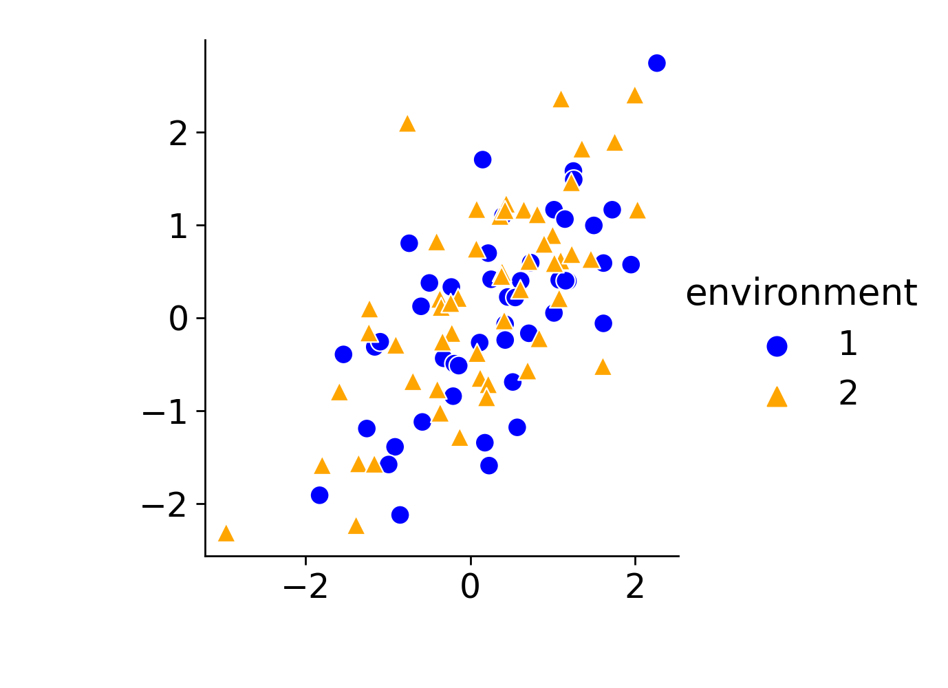
       EIIL

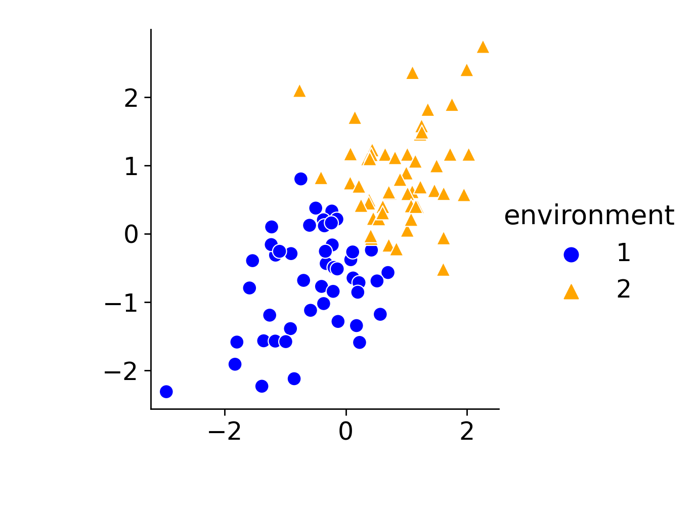
       $k$-means

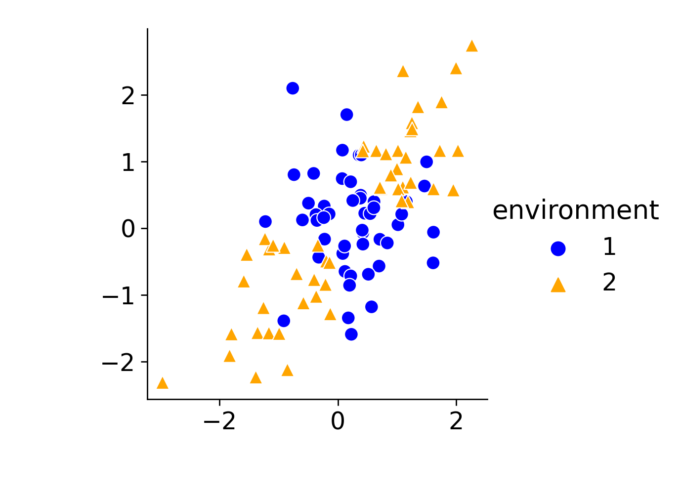
       Decorr

Figure 1: Partitioning results of two environments given by different methods on a toy dataset.

5 Experiments

We evaluate four different environment partitioning methods: pure random, EIIL (Creager et al., 2021), $k$-means, and Decorr for IRM, and the whole procedure of HRM (Heterogeneous Risk Minimization, Liu et al. (2021b)) on some experiments. Meanwhile, we also implement the original IRM (and V-REx (Krueger et al., 2021) in real data experiments only) when environments naturally exist, and ERM for comparison as well. In all experiments, we set $p_{0}=0.1$, $\alpha=0.1$, $T=5000$, and $\lambda=100$ for Decorr and set different $k$ for different situations. For example, in synthetic data experiments, $k$ is the true number of environments in training data (from 2 to 8). In most cases, $k=2$ or $3$ in our experiments. Comparatively, in related works such as EIIL, HRM, or those using $k$-means, the number of training environments was set to be 2 or 3. We use the original or popular implementations of IRM, EIIL, and HRM.

Although dealing with image data is not the main purpose of this paper, we also implement Decorr on two image datasets CMNIST and Waterbirds to show that our method is capable of applying on different types of datasets. The results on image datasets are shown in Appendix A, in which the success of Decorr is exhibited.

5.1 Synthetic Data Experiments

IRM example.

Following Aubin et al. (2021), we test the performance of different methods on IRM example generated by Equation (3) with $W_{xy}=W_{yx}=I$ and $\sigma^{e}=0.1,~{}1.5,~{}2$ for three different $e$. In each environment $e$, 1,000 samples are generated. We want the model to learn the true causal relation, which is $y=1^{T}_{d}x_{1}+\epsilon$, instead of using the spurious correlation between $x_{2}$ and $y$. So we evaluate the performance of models by calculating MSE between linear regression coefficients and the ground-truth coefficients $\beta^{*}=(1_{d},0_{d})$. We evaluate in cases with different numbers of original environments (e.g., the first two $\sigma^{e}$) and different data dimensions $d$. The penalty weight is $\beta=10$ for IRM. Results are shown in Table 1, with 10 trials to calculate the standard deviation. In most cases, Decorr provides the closest coefficients to $\beta^{*}$. Original IRM (the last row) with known true environments certainly can produce the true coefficients.

Table 1: IRM example: MSE between linear regression coefficients and the ground truth.

	number of envs $=2$				number of envs $=3$
Method	$d=2$	$d=5$	$d=10$	$d=20$	$d=2$	$d=5$	$d=10$	$d=20$
ERM	0.28(0.01)	0.28(0.02)	0.29(0.02)	0.28(0.02)	0.46(0.01)	0.46(0.01)	0.46(0.02)	0.46(0.02)
random+IRM	0.28(0.06)	0.27(0.04)	0.27(0.02)	0.29(0.02)	0.45(0.06)	0.49(0.10)	0.49(0.04)	0.46(0.04)
EIIL	0.29(0.05)	0.35(0.06)	0.36(0.03)	0.38(0.04)	0.17(0.08)	0.31(0.08)	0.34(0.03)	0.37(0.04)
$k$-means+IRM	0.21(0.05)	0.27(0.04)	0.27(0.03)	0.28(0.02)	0.33(0.08)	0.33(0.10)	0.38(0.07)	0.35(0.04)
HRM	0.38(0.17)	0.43(0.06)	0.44(0.04)	0.47(0.02)	0.50(0.00)	0.50(0.00)	0.50(0.00)	0.49(0.01)
Decorr (ours)	0.13(0.03)	0.16(0.09)	0.16(0.06)	0.09(0.02)	0.25(0.02)	0.29(0.04)	0.26(0.05)	0.25(0.03)
IRM (oracle)	0.02(0.00)	0.02(0.01)	0.02(0.00)	0.02(0.00)	0.07(0.03)	0.04(0.01)	0.04(0.02)	0.02(0.00)

Risks of IRM.

Next, we do the experiment on data generated by Equation (4) and (5). We let the number of environments in training data vary from 2 to 8, and for each case, do training and testing 10 times for averaging for evaluating different methods. The results are shown in Figure 4. In each training and testing, the settings are $\eta=0.5$, $\mu_{c}=Z_{1}+0.5sign(Z_{1})$, $\mu_{e}=1.5Z_{2}+Z_{e}$, $\sigma_{c}^{2}=2$, $\sigma_{e}^{2}=0.1$, where $Z_{1}\in\mathbb{R}^{3},Z_{2}\in\mathbb{R}^{6},Z_{e}\in\mathbb{R}^{6}$ are all sampled from standard normal. $Z_{1},Z_{2}$ are shared across environments and $Z_{e}$ is not. In each environment $e$, we sample 1,000 points. After training with the fixed number of environments, 5,000 different test environments (5,000 different new $Z_{e}$) are generated to compute the worst-case error with them. In this experiment, $f$ is the identity function and logistic classifiers are learned. The penalty weight is $\beta=10^{4}$ for IRM. Most of the hyper-parameters are the same as in the experiment in Rosenfeld et al. (2020), except an additional $sign(Z_{1})$ term to make invariant features worth learning, and a lower $\sigma_{e}^{2}$ to make it more difficult to capture invariant features. Figure 4 shows that Decorr can produce stable low error rate.

5.2 Real Data Experiments

Implementation details.

For each task, we use MLPs with two hidden layers with tanh activations and dropout ($p=0.5$) after each hidden layer. The size of each hidden layer is $2^{int(\log_{2}p)+2}$, where $p$ is the input dimension. The output layer is linear or logistic. We optimize the binary cross-entropy loss for classification and MSE for regression using Adam (Kingma & Ba, 2015) with default settings (learning rate $=0.001$, $\beta_{1}=0.9$, $\beta_{2}=0.999$, $\epsilon=10^{-8}$). $n_{iter}=20000$ and an $L_{2}$ penalty term with weight 0.001 is added. For IRM, the penalty weight is $\beta=10^{4}$. Except for occupancy estimation, all the other experiments use $k=2$ for Decorr and other methods. If not mentioned, the original environment partitions for IRM and REx are naturally decided by timestamps of the observations.

Financial indicators.

The task for financial indicators dataset is to predict if the price of a stock will increase in the next whole year, given the financial indicators of the stock. The dataset is split into five years from 2014 to 2018. We follow the implementation details in Krueger et al. (2021), consider each year as a baseline environment, and use any three environments as the training set, one environment as the validation set for early stopping, and one environment as the testing set. There is a set of 20 different tasks in total. We also collect another set of 20 tasks, using only one environment as the training set, one as the validation set, and three as the testing set in each task. The original IRM and REx cannot work now because there is only one explicit environment in training data. We follow Shen et al. (2021), evaluate all methods with average error rate, worst-case error rate, and standard deviation on these two task sets. Results are shown in Table 2, where Decorr wins the best performance.

Table 2: Financial indicators: task set 1 uses three environments as training set, and task set 2 uses one environment as training set.

	Task Set 1			Task Set 2
Method	Avg. Error	Worst Error	STD	Avg. Error	Worst Error	STD
ERM	45.02(0.00)	52.92(0.12)	5.20	46.79(0.01)	51.05(0.05)	2.44
random+IRM	45.95(0.28)	53.77(0.58)	4.27	46.57(0.26)	52.03(0.79)	2.57
EIIL	48.95(0.16)	57.37(0.65)	4.52	48.97(0.38)	54.62(0.70)	2.71
$k$-means+IRM	45.20(0.34)	53.64(0.44)	6.19	46.79(0.28)	54.72(1.22)	3.43
HRM	44.64(0.00)	53.52(0.03)	5.71	46.71(0.00)	51.17(0.00)	2.48
Decorr (ours)	43.99(0.10)	51.61(0.04)	5.33	43.96(0.25)	50.23(1.17)	2.81
IRM	45.86(0.14)	56.38(0.21)	6.27
V-REx	44.08(0.02)	55.41(0.12)	6.30

Adult.

Adult is a tabular dataset extracted from a census in USA. The task is to classify if the individual’s yearly income is above or below 50,000 USD based on given characteristics. We remove all the categorical variables except race and sex, both of which are transformed into binary values $\{0,1\}$. To make a distributional shift from training data to testing data, we sample from the data as follows. First we choose the race or sex as the biased feature, denoted as $x^{b}$, and split the whole dataset into four groups: $\{x^{b}=0,y=0\}$, $\{x^{b}=1,y=1\}$, $\{x^{b}=0,y=1\}$, and $\{x^{b}=1,y=0\}$. For the training set, we use 90% of the data in the first two groups but only use $\alpha$ proposition of the data in the last two groups. The remaining data goes to the testing set. Lower $\alpha$ leads to a greater distributional shift, and when $\alpha$ rises to 0.9, there is no distributional shift at all. We expect those IRM-based methods to learn the spurious correlation ($x^{b}=1$ causes $y=1$) under small $\alpha$. Error rate results are shown in Figure 4 and 4. Original environments are decided by the biased feature.

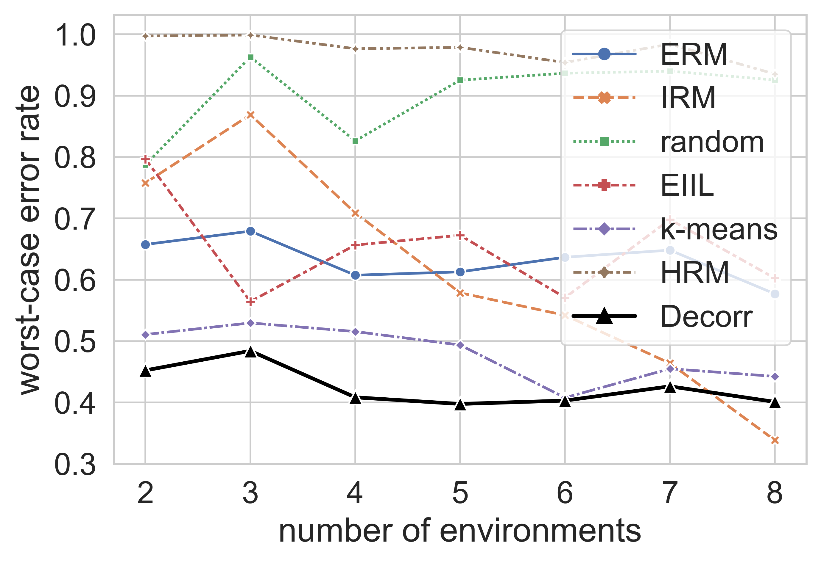
Figure 2: Risks of IRM.

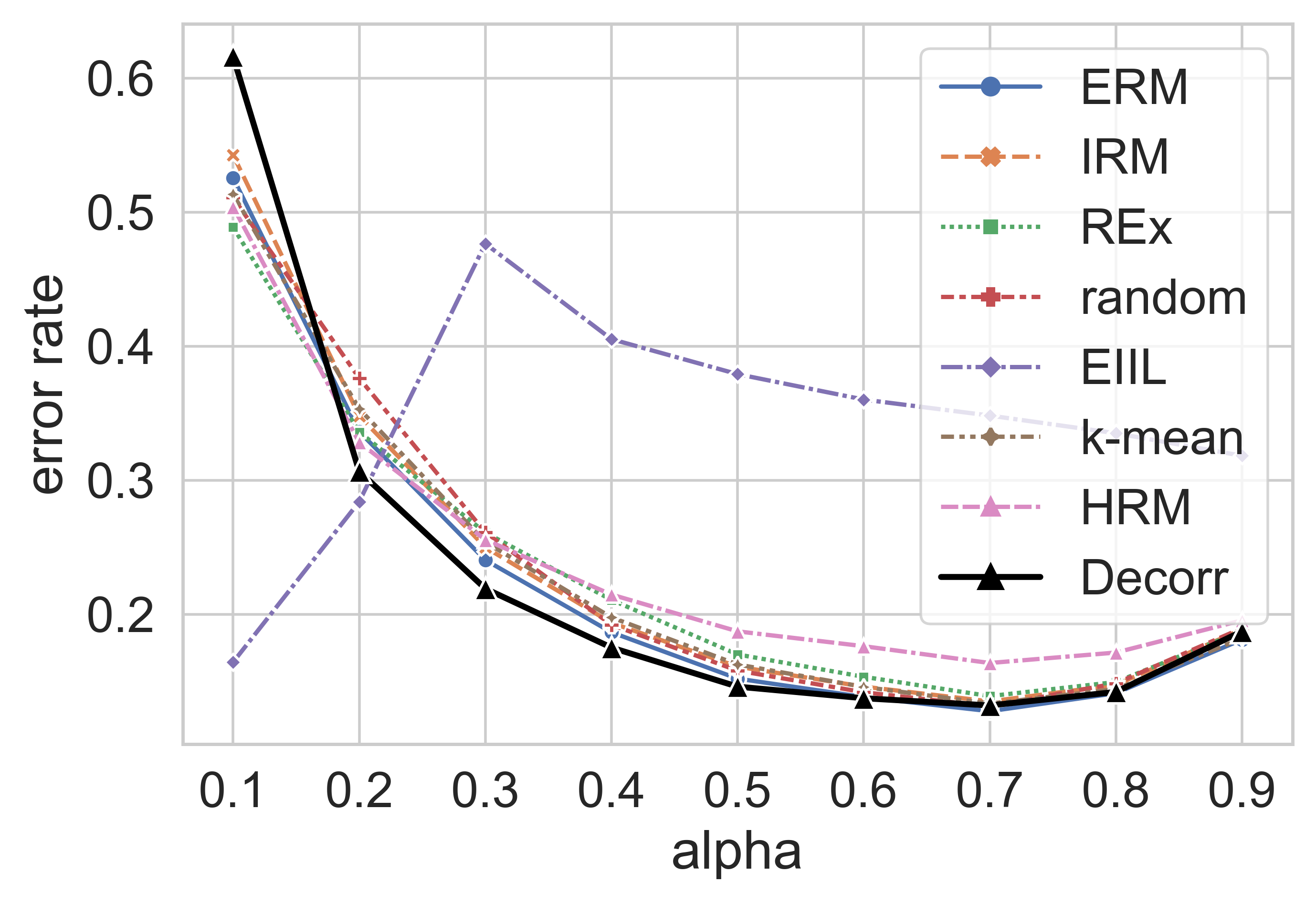
Figure 3: Adult: using race
as the bias feature.

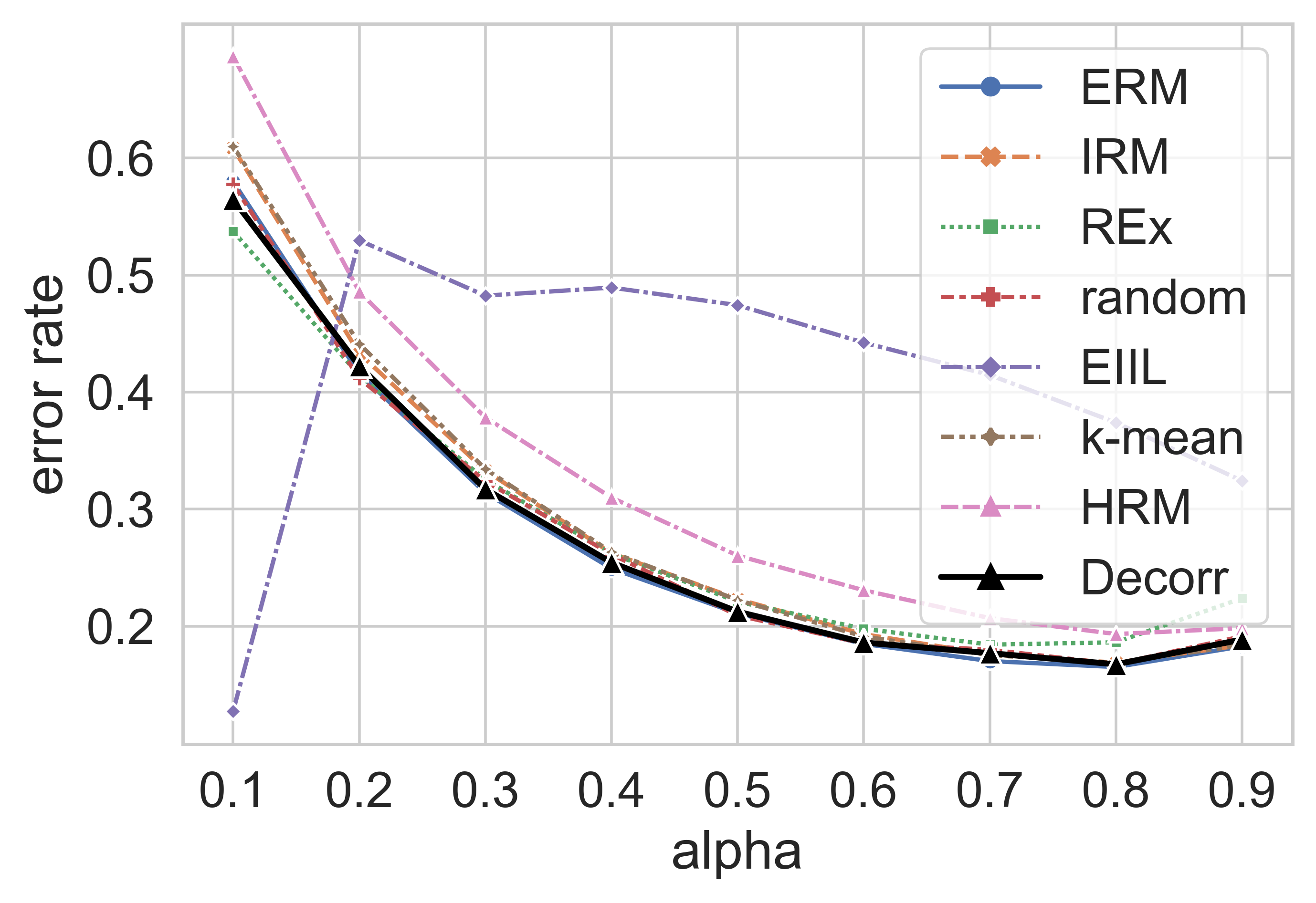
Figure 4: Adult: using sex
as the bias feature.

Occupancy estimation.

Occupancy estimation dataset contains data from different types of sensors (temperature, light, sound, CO2, etc.) in a room every minute. The task is to estimate the occupancy in the room varying between 0 and 3 people. We regard this as a regression task, transform the time into real numbers in $[0,1]$, standardized the features, and train the models with the given training and testing sets. The training errors are high for all the environment partitioning methods when $k=2$, so we set $k=3$ and the MSE on testing set are shown in Table LABEL:occupancy. Decorr again performs the best on the testing error. Original environments are decided by the collection time of the samples.

Table 3: Occupancy Estimation

Method	Training Error	Testing Error
ERM	0.026(0.000)	0.773(0.000)
random+IRM	0.587(0.053)	0.824(0.093)
EIIL	0.191(0.203)	0.690(0.048)
$k$-means+IRM	0.044(0.001)	0.352(0.009)
HRM	0.166(0.000)	1.154(0.000)
Decorr (ours)	0.143(0.009)	0.268(0.011)
IRM	0.420(0.006)	0.840(0.021)
V-REx	0.060(0.001)	0.686(0.030)

Table 4: Stock

Method	Average Error	Worst-Case Error	STD
ERM	50.33(0.10)	56.65(0.26)	3.86
random+IRM	50.11(0.35)	54.54(0.81)	2.62
EIIL	49.70(0.33)	52.29(0.44)	1.65
$k$-means+IRM	50.02(0.30)	54.92(0.23)	2.68
HRM	50.22(0.00)	55.97(0.00)	4.78
Decorr (ours)	49.13(0.34)	53.50(0.75)	3.66

Stock.

Stock dataset contains market data and technical indicators of 10 US stocks from 2005 to 2020. We try to use technical indicators today to predict whether the close price of one stock tomorrow is higher than today’s. For each stock, we use the first 70% of the data as training set, 10% as validation set for early stopping, and the last 20% as testing set. The modeling is done stock-wisely. Again, we evaluate methods by average error rate, worst-case error rate, and standard deviation across different stocks. Results are shown in Table 5.2, where we can see Decorr performs the best on the average error. Because there are no original environments, the original IRM and REx are not applied.

5.3 Summary

In this section, we briefly summarize the characteristics of the tested methods. IRM has excellent performance with environment partition that reflects the true data-generating mechanics. However, usually it is not the case in most of the real datasets. We can see that the simple and natural split-by-time partition has no significant advantage compared to ERM. While EIIL has good performance on image data, our experiments show that it may not be suitable for some other types of data. Too much noise can indeed affect the performance of this mistake-exploration method greatly, just as we mentioned in the introduction section.

$k$-means is an easy and direct way to do environment partitioning and has consistently good performance in several experiments. However, the illustration in Figure 1 shows that $k$-means may not be the optimal partitioning method. Our Decorr algorithm achieves the best performance overall in the above experiments. We notice that Decorr does not recover the original data sources, but tries to find a partition that outperforms the original/natural partition instead.

6 Conclusion

Invariant learning is an effective framework for OOD generalization. Environment partitioning is indeed an important problem for invariant learning, and crucially determines the performance of IRM. While existing partitioning methods have good OOD generalization performance on image data, we show that the performance does not hold on some other types of data. Motivated by the benefits of low-correlated training set, we propose Decorr algorithm to split the data into several environments with low correlation inside. We also theoretically prove that uncorrelated environments make OOD generalization easier. Our environment partitioning method has advantages over the existing ones. Across different types of tasks (including image tasks), we verify that our method can significantly and consistently improve the performance of IRM, making IRM more generally applicable.

Appendix A Image Data Experiments

To show that our method is applicable on different types of data, we implement Decorr and other baseline methods on two image datasets. With some minor modifications on Decorr based on the characteristics of image data, our method can outperform others as well. Unless stated otherwise, the implementation details are the same as in Section 5.2.

Decorr for images.

Image data have much higher dimensions than tabular data. Therefore, directly decorrelate the raw image data is not applicable. We need to extract features before the process of decorrelation. We train a convolutional neural network or MLP (just as we do in ERM) and take the output of the last full-connection layer as the features of the data. With these low-dimensional extracted features, we can now do decorrelation as before (we also implement $k$-means in this way). After the dataset partitioning, we still use the raw image data for IRM training. For Decorr, we do not impose the restriction of same sample size for partitioned environments (i.e., $\lambda=0$ in Algorithm 1), so that Decorr can split image datasets into more diversified environments.

A.1 Colored MNIST

Colored MNIST (CMNIST), proposed by Arjovsky et al. (2020) to validate IRM’s ability to learn nonlinear invariant predictors, is an image dataset derived from MNIST. CMNIST is constructed by coloring each MNIST image into red or green and making the image’s color strongly but spuriously correlates with the class label. Regular deep learning models would fail, for they will classify the image by color rather than shape.

In detail, CMNIST is a binary classification task. We follow the construction of CMNIST in Arjovsky et al. (2020). Images are first labeled $\tilde{y}=0$ for digits 0-4 and $\tilde{y}=1$ for digits 5-9. Then the final label $y$ is obtained by flipping $\tilde{y}$ with probability $0.1$ (can be regarded as data noise). Next, they sample the color ID $z$ by flipping $y$ with probability $p^{e}$, where $p^{e}=0.2$ in the first training environment and 0.1 in the second. However, $p^{e}=0.9$ for the test environment, implying a huge converse in the correlation between color and label. Finally, they color the images based on their color ID $z$. Please see Figure 6 and 6 for an intuitive illustration.

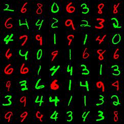
Figure 5: CMNIST training set: most of 0-4 are green, most of 5-9 are red.

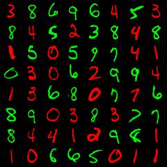
Figure 6: CMNIST testing set: most of 0-4 are red, most of 5-9 are green.

Following Arjovsky et al. (2020), we use an MLP with two hidden layers as our base model. The architecture of the network and all the hyperparameters are the same. We evaluate the error rate on the testing set as well as the percentage of data with rare patterns (i.e., red, labeled in 0-4; or green, labeled in 5-9) in each partitioned environment. If the percentages of two environments have a huge gap, the environments are more diversified, which is better for invariant learning. Each model is trained for 5000 epochs, of which the first 100 epochs are trained without IRM penalty. The results are shown in Table 5, where the superiority of Decorr is illustrated.

Table 5: CMNIST error rate on testing set and the percentage of rare patterns in each of the two partitioned environments.

		% of rare patterns
Method	Average Error	Environment 1	Environment 2
ERM	43.33(0.14)	————–	————–
random+IRM	40.16(0.16)	15.15(0.08)	14.83(0.10)
EIIL	76.95(3.46)	29.59(2.14)	14.07(0.09)
$k$-means+IRM	41.93(0.52)	15.32(0.21)	14.68(0.19)
Decorr (ours)	34.89(6.24)	40.24(0.49)	4.72(0.26)
IRM (oracle)	30.18(0.94)	19.89(0.13)	10.09(0.12)
V-REx (oracle)	34.22(0.04)	19.89(0.13)	10.09(0.12)

A.2 Waterbirds

Waterbirds dataset is proposed by Sagawa et al. (2019). It is a dataset that combines the CUB dataset (Wah et al., 2011) and the Places dataset (Zhou et al., 2017). The task is to predict the type of bird (waterbird or landbird) from the CUB dataset. However, the combination of CUB and Places produces a spurious correlation. In the training set, most of the landbirds are in land backgrounds, and most of the waterbirds are in water backgrounds. 95% of the data are in this regular pattern. Nevertheless, in the testing set, only half of the data are in this regular pattern, and the other half are not. So the correlation in training set does not exist anymore. More details about the dataset can be found in Sagawa et al. (2019).

Following Sagawa et al. (2019), we use pretrained ResNet50 as our base model, and the $L_{2}$ penalty weight is set to be $10^{-4}$. Each model is trained for 50 epochs. We also implement IRM and V-REx with the optimal environment partition: one environment consists of all the regular pattern data (waterbirds in water and landbirds in land), and the other one consists of all the rare pattern data. We implement each method and report the error rate. The results are shown in Table 6, in which Decorrr gives the best performance among all partitioning methods.

Table 6: Waterbirds error rate on testing set.

Method	Average Error
ERM	25.76(0.23)
random+IRM	22.96(0.43)
EIIL	27.43(7.25)
$k$-means+IRM	24.32(0.65)
Decorr (ours)	22.70(0.44)
IRM (oracle)	22.36(0.08)
V-REx (oracle)	33.53(7.84)

References

- Ahmed et al. (2020) Faruk Ahmed, Yoshua Bengio, Harm van Seijen, and Aaron Courville. Systematic generalisation with group invariant predictions. In International Conference on Learning Representations, 2020.
- Ahuja et al. (2020) Kartik Ahuja, Karthikeyan Shanmugam, Kush Varshney, and Amit Dhurandhar. Invariant risk minimization games. In International Conference on Machine Learning, pp. 145–155. PMLR, 2020.
- Arjovsky et al. (2020) Martin Arjovsky, Léon Bottou, Ishaan Gulrajani, and David Lopez-Paz. Invariant risk minimization. stat, 1050:27, 2020.
- Aubin et al. (2021) Benjamin Aubin, Agnieszka Słowik, Martin Arjovsky, Leon Bottou, and David Lopez-Paz. Linear unit-tests for invariance discovery. arXiv preprint arXiv:2102.10867, 2021.
- Blessie & Karthikeyan (2012) E Chandra Blessie and E Karthikeyan. Sigmis: a feature selection algorithm using correlation based method. Journal of Algorithms & Computational Technology, 6(3):385–394, 2012.
- Chattopadhyay et al. (2020) Prithvijit Chattopadhyay, Yogesh Balaji, and Judy Hoffman. Learning to balance specificity and invariance for in and out of domain generalization. In European Conference on Computer Vision, pp. 301–318. Springer, 2020.
- Costa (2011) Joaquim F. Pinto da Costa. Weighted Correlation, pp. 1653–1655. Springer Berlin Heidelberg, Berlin, Heidelberg, 2011. ISBN 978-3-642-04898-2. doi: 10.1007/978-3-642-04898-2_612. URL https://doi.org/10.1007/978-3-642-04898-2_612.
- Creager et al. (2021) Elliot Creager, Jörn-Henrik Jacobsen, and Richard Zemel. Environment inference for invariant learning. In International Conference on Machine Learning, pp. 2189–2200. PMLR, 2021.
- Dagaev et al. (2021) Nikolay Dagaev, Brett D Roads, Xiaoliang Luo, Daniel N Barry, Kaustubh R Patil, and Bradley C Love. A too-good-to-be-true prior to reduce shortcut reliance. arXiv preprint arXiv:2102.06406, 2021.
- Geirhos et al. (2020) Robert Geirhos, Jörn-Henrik Jacobsen, Claudio Michaelis, Richard Zemel, Wieland Brendel, Matthias Bethge, and Felix A Wichmann. Shortcut learning in deep neural networks. Nature Machine Intelligence, 2(11):665–673, 2020.
- Hall (2000) Mark A Hall. Correlation-based feature selection of discrete and numeric class machine learning. 2000.
- Hall et al. (1999) Mark Andrew Hall et al. Correlation-based feature selection for machine learning. 1999.
- Kingma & Ba (2015) Diederik P Kingma and Jimmy Ba. Adam: A method for stochastic optimization. In International Conference on Learning Representations, 2015.
- Krueger et al. (2021) David Krueger, Ethan Caballero, Joern-Henrik Jacobsen, Amy Zhang, Jonathan Binas, Dinghuai Zhang, Remi Le Priol, and Aaron Courville. Out-of-distribution generalization via risk extrapolation (rex). In International Conference on Machine Learning, pp. 5815–5826. PMLR, 2021.
- Kuang et al. (2020) Kun Kuang, Ruoxuan Xiong, Peng Cui, Susan Athey, and Bo Li. Stable prediction with model misspecification and agnostic distribution shift. In Proceedings of the AAAI Conference on Artificial Intelligence, volume 34, pp. 4485–4492, 2020.
- Liu et al. (2021a) Evan Z Liu, Behzad Haghgoo, Annie S Chen, Aditi Raghunathan, Pang Wei Koh, Shiori Sagawa, Percy Liang, and Chelsea Finn. Just train twice: Improving group robustness without training group information. In International Conference on Machine Learning, pp. 6781–6792. PMLR, 2021a.
- Liu et al. (2021b) Jiashuo Liu, Zheyuan Hu, Peng Cui, Bo Li, and Zheyan Shen. Heterogeneous risk minimization. In International Conference on Machine Learning, pp. 6804–6814. PMLR, 2021b.
- Lu et al. (2021) Chaochao Lu, Yuhuai Wu, Jośe Miguel Hernández-Lobato, and Bernhard Schölkopf. Nonlinear invariant risk minimization: A causal approach. arXiv preprint arXiv:2102.12353, 2021.
- Matsuura & Harada (2020) Toshihiko Matsuura and Tatsuya Harada. Domain generalization using a mixture of multiple latent domains. In Proceedings of the AAAI Conference on Artificial Intelligence, volume 34, pp. 11749–11756, 2020.
- Nam et al. (2020) Junhyun Nam, Hyuntak Cha, Sungsoo Ahn, Jaeho Lee, and Jinwoo Shin. Learning from failure: De-biasing classifier from biased classifier. Advances in Neural Information Processing Systems, 33:20673–20684, 2020.
- Rosenfeld et al. (2020) Elan Rosenfeld, Pradeep Kumar Ravikumar, and Andrej Risteski. The risks of invariant risk minimization. In International Conference on Learning Representations, 2020.
- Sagawa et al. (2019) Shiori Sagawa, Pang Wei Koh, Tatsunori B Hashimoto, and Percy Liang. Distributionally robust neural networks for group shifts: On the importance of regularization for worst-case generalization. arXiv preprint arXiv:1911.08731, 2019.
- Shen et al. (2020) Zheyan Shen, Peng Cui, Jiashuo Liu, Tong Zhang, Bo Li, and Zhitang Chen. Stable learning via differentiated variable decorrelation. In Proceedings of the 26th acm sigkdd international conference on knowledge discovery & data mining, pp. 2185–2193, 2020.
- Shen et al. (2021) Zheyan Shen, Jiashuo Liu, Yue He, Xingxuan Zhang, Renzhe Xu, Han Yu, and Peng Cui. Towards out-of-distribution generalization: A survey. arXiv preprint arXiv:2108.13624, 2021.
- Sohoni et al. (2020) Nimit Sohoni, Jared Dunnmon, Geoffrey Angus, Albert Gu, and Christopher Ré. No subclass left behind: Fine-grained robustness in coarse-grained classification problems. Advances in Neural Information Processing Systems, 33:19339–19352, 2020.
- Thopalli et al. (2021) Kowshik Thopalli, Sameeksha Katoch, Andreas Spanias, Pavan Turaga, and Jayaraman J Thiagarajan. Improving multi-domain generalization through domain re-labeling. arXiv preprint arXiv:2112.09802, 2021.
- Wah et al. (2011) Catherine Wah, Steve Branson, Peter Welinder, Pietro Perona, and Serge Belongie. The caltech-ucsd birds-200-2011 dataset. 2011.
- Wright (1921) Wright. Correlation and causation. Journal of agricultural research., 20(3), 1921. ISSN 0095-9758.
- Ye et al. (2021) Nanyang Ye, Kaican Li, Lanqing Hong, Haoyue Bai, Yiting Chen, Fengwei Zhou, and Zhenguo Li. Ood-bench: Benchmarking and understanding out-of-distribution generalization datasets and algorithms. arXiv preprint arXiv:2106.03721, 2021.
- Yu & Liu (2003) Lei Yu and Huan Liu. Feature selection for high-dimensional data: A fast correlation-based filter solution. In Proceedings of the 20th international conference on machine learning (ICML-03), pp. 856–863, 2003.
- Zhang et al. (2021) Xingxuan Zhang, Peng Cui, Renzhe Xu, Linjun Zhou, Yue He, and Zheyan Shen. Deep stable learning for out-of-distribution generalization. In Proceedings of the IEEE/CVF Conference on Computer Vision and Pattern Recognition, pp. 5372–5382, 2021.
- Zhou et al. (2017) Bolei Zhou, Agata Lapedriza, Aditya Khosla, Aude Oliva, and Antonio Torralba. Places: A 10 million image database for scene recognition. IEEE transactions on pattern analysis and machine intelligence, 40(6):1452–1464, 2017.
- Zhou et al. (2021) Kaiyang Zhou, Ziwei Liu, Yu Qiao, Tao Xiang, and Chen Change Loy. Domain generalization: A survey. 2021.