Curing the Divergence in Time-Dependent Density Functional Quadratic Response Theory

Abstract

The adiabatic approximation in time-dependent density functional theory (TDDFT) is known to give an incorrect pole structure in the quadratic response function, leading to unphysical divergences in excited state-to-state transition probabilities and hyperpolarizabilties. We find the form of the exact quadratic response kernel and derive a practical and accurate approximation that cures the divergence. We demonstrate our results on excited state-to-state transition probabilities of a model system and of the LiH molecule.

Until recently, quadratic response has received far less attention than linear response. Most response applications had involved properties related to the optical spectra of a molecule in equilibrium, while relatively few ventured into non-linear regime to gain access to properties such as two-photon absorption, sum-frequency generation, and hyperpolarizabilities which can be obtained from the quadratic response of the ground-state system Papadopoulos et al. (2006); Mukamel (1999). However, in the past few decades, non-linear optical processes have emerged as key in a number of applications, including optical data storage and switching, for examples. Moreover, an increasingly relevant class of applications involve excited-state dynamics, where a molecule is initially photo-excited and coupled electron-ion motion ensues. Such applications inherently require the response of an excited state, appearing in the form of excited state-to-state transition amplitudes. These amplitudes also appear even without nuclear motion: when simulating the dynamics of a molecule in a non-perturbative laser field by expressing the wavefunction in a superposition of eigenstates, coupled by the laser field.

Response theory offers a way to obtain these quantities by circumventing the expensive calculation of the excited-state wavefunctions, and may yield more accurate properties when, inevitably, approximations are used. However, response theories of approximate electronic structure theories suffer from an unphysical divergence problem when the difference between two excitation frequencies is equal to another excitation frequency Parker et al. (2016). This had been first discovered in time-dependent Hartree-Fock (TDHF) forty years ago Dalgaard (1982) but lay relatively dormant until the work of Ref. Parker et al. (2016) which showed the divergence also appears in response theories based on coupled-cluster, multi-configuration self-consistent field, and in adiabatic time-dependent density functional theory (TDDFT) Li and Liu (2014); Ou et al. (2015a); Zhang and Herbert (2015); Parker et al. (2016).

Addressing this issue for TDDFT Runge and Gross (1984); Ullrich (2011); Marques et al. (2012); Maitra (2016) is of great interest: not only does TDDFT have a favorable system-size scaling enabling the calculation of photo-induced dynamics in complex molecules, it is in principle an exact theory and so offers the possibility of finding more accurate functional approximations that cure the unphysical divergence, which is what we aim to achieve here.

We find the form of the exact quadratic response kernel of TDDFT and show explicitly why the adiabatic approximations used thus far are responsible for the incorrect pole structure of the second-order response function that creates the divergence, and that a relatively gentle linear frequency-dependence in the quadratic response kernel corrects the pole structure and tames the divergence. Inspired by this, we derive a frequency-dependent approximation for the quadratic response kernel. Results on a two-electron model system and on the LiH molecule show that our approximation provides a practical and accurate fix to the problem of divergences in TDDFT quadratic response.

In TDDFT response theory, the central object at each order of response is a density-response function expressed in terms of response functions of the Kohn-Sham (KS) system, and exchange-correlation kernels Gross et al. (1996); Marques et al. (2012). The linear density response function of the interacting system to an external perturbation $\delta v_{\rm ext}({\bf r},t)$, $\chi({\bf r},{\bf r}^{\prime},t-t^{\prime})=\frac{\delta n({\bf r},t)}{\delta v_{\rm ext}({\bf r}^{\prime}t^{\prime})}=-i\theta(t-t^{\prime})\langle\Psi_{0}|[\hat{n}({\bf r}t),\hat{n}({\bf r}^{\prime}t^{\prime})]|\Psi_{0}\rangle$, where $\theta(t-t^{\prime})$ is the step function, has the spectral representation

$$\chi({\bf r},{\bf r}^{\prime},\omega)=\sum_{a}\left(\frac{n_{0a}({\bf r})n_{a0}({\bf r}^{\prime})}{\omega-\Omega_{a}+i0^{+}}\,-\,\frac{n_{0a}({\bf r}^{\prime})n_{a0}({\bf r})}{\omega+\Omega_{a}+i0^{+}}\right)$$ (1)

where $n_{0a}({\bf r})=\langle\Psi_{0}|\hat{n}({\bf r})|\Psi_{a}\rangle$ is the transition density between the ground state, $\Psi_{0}$ and the excited state, $\Psi_{a}$ which has excitation frequency $\Omega_{a}=E_{a}-E_{0}$ and $\hat{n}({\bf r})$ is the one-body density-operator; the $0^{+}$ indicates the shift of the pole slightly below the real-axis to ensure causality and will be omitted hereon. In TDDFT, $\chi$ is instead obtained from the non-interacting KS system, through the Dyson-like equation Petersilka et al. (1996); Casida (1995)

$$\chi^{\rm tddft}_{ij}(\omega)=\chi_{{\scriptscriptstyle\rm S},ij}(\omega)+\chi_{{\scriptscriptstyle\rm S},ik}(\omega)f_{{}_{\scriptscriptstyle\rm HXC},kl}(\omega)\chi_{lj}(\omega)$$ (2)

where $\chi_{{\scriptscriptstyle\rm S}}$ is the density response function of the KS system and $f_{\scriptscriptstyle\rm HXC}(\omega)$ is the Hartree-exchange correlation kernel. The indices $i,j$ represent the spatial variables ${\bf r}_{i}$ and ${\bf r}_{j}$ and repeated indices imply integration. While $\chi_{\scriptscriptstyle\rm S}(\omega)$ displays residues given by transition-densities between ground and excited states of the KS system, and poles given by KS excitation frequencies, the linear response (LR) kernel, $f_{{}_{\scriptscriptstyle\rm HXC},kl}[n_{0}](t-t^{\prime})=\frac{\delta(t-t^{\prime})}{|{\bf r}_{k}-{\bf r}_{l}|}+\left.\frac{\delta v_{\scriptscriptstyle\rm XC}[n]({\bf r}_{k},t)}{\delta n({\bf r}_{l},t^{\prime})}\right|_{n=n_{0}}$, corrects these to those of the true response function. Almost always, an adiabatic approximation is used, where the exchange-correlation potential $v_{\scriptscriptstyle\rm XC}[n]({\bf r},t)$ depends only on the instantaneous density and is approximated by the functional derivative of a ground-state energy functional, $E_{\scriptscriptstyle\rm XC}[n]$. This results in a frequency-independent kernel, $f_{{\scriptscriptstyle\rm XC},ij}^{\rm adia}[n](\omega)=\frac{\delta^{2}E_{\scriptscriptstyle\rm XC}[n]}{\delta n({\bf r}_{i})\delta n({\bf r}_{j})}$. With an adiabatic approximation, LR TDDFT has become a workhorse of electronic structure calculations, yielding excitation spectra with an unprecedented balance between accuracy and efficiency. The adiabatic approximation is known to fail for certain classes of excitations, and improved, frequency-dependent, approximations have been derived for some cases, e.g. double-excitations Maitra et al. (2004); Maitra (2022).

Going to second-order in the perturbation, defines the quadratic response (QR) function Wehrum and Hermeking (1974); Gross et al. (1996); Senatore and Subbaswamy (1987), $\chi^{(2)}({\bf r},{\bf r}_{1},{\bf r}_{2},t-t_{1},t-t_{2})=\frac{\delta^{2}n({\bf r},t)}{\delta v_{\rm ext}({\bf r}_{1},t_{1})\delta v_{\rm ext}({\bf r}_{2},t_{2})}$:

$$\chi^{(2)}({\bf r},{\bf r}_{1},{\bf r}_{2};t-t_{1},t-t_{2})=\frac{(-i)^{2}}{2}\theta(t-t_{1})\theta(t_{1}-t_{2})\\ \times\langle\Psi_{0}|\left[\left[\hat{n}({\bf r},t),\hat{n}({\bf r}_{1},t_{1})\right],\hat{n}({\bf r}_{2},t_{2})\right]|\Psi_{0}\rangle\,+\,\,(1\leftrightarrow 2)$$ (3)

which has the spectral representation Senatore and Subbaswamy (1987)

$$\chi^{(2)}({\bf r},{\bf r}_{i},{\bf r}_{j},\omega_{i},\omega_{j})=\frac{1}{2}\sum_{a,b}\left(\frac{n_{0a}({\bf r})n_{ab}({\bf r}_{i})n_{b0}({\bf r}_{j})}{(\omega_{i}+\omega_{j}-\Omega_{b})(\omega_{j}-\Omega_{a})}-\frac{n_{0a}({\bf r}_{j})n_{ab}({\bf r})n_{b0}({\bf r}_{i})}{(\omega_{i}-\Omega_{b})(\omega_{j}+\Omega_{a})}+\frac{n_{0a}({\bf r}_{j})n_{ab}({\bf r}_{i})n_{b0}({\bf r})}{(\omega_{i}+\omega_{j}+\Omega_{b})(\omega_{i}+\Omega_{a})}+\,(i\leftrightarrow j)\right)$$ (4)

where the state-$a$ to state-$b$ transition density is $n_{ab}({\bf r})=\langle\Psi_{a}|\hat{n}({\bf r})|\Psi_{b}\rangle$, and can be extracted from double residues of $\chi^{(2)}$. The second-order response may be extracted from TDDFT linear response quantities together with a QR kernel $g_{\scriptscriptstyle\rm XC}({\bf r},{\bf r}_{1},{\bf r}_{2},t-t_{1},t-t_{2})=\left.\frac{\delta^{2}v_{\scriptscriptstyle\rm XC}({\bf r},t)}{\delta n({\bf r}_{1},t_{1})\delta n({\bf r}_{2},t_{2})}\right|_{n_{0}}$ through Gross et al. (1996); Parker and Furche (2018); Sałek et al. (2002):

$$\chi_{mnp}^{(2),{\rm tddft}}(\omega_{1},\omega_{2})=\chi_{mi}(\omega_{1}+\omega_{2})\chi_{{\scriptscriptstyle\rm S},ij}^{-1}(\omega_{1}+\omega_{2})\chi_{{\scriptscriptstyle\rm S},jkl}^{(2)}(\omega_{1},\omega_{2})\chi_{{\scriptscriptstyle\rm S},lq}^{-1}(\omega_{1})\chi_{qn}(\omega_{1})\chi_{{\scriptscriptstyle\rm S},kr}^{-1}(\omega_{2})\chi_{rp}(\omega_{2})\\ +\chi_{mi}(\omega_{1}+\omega_{2})g_{{\scriptscriptstyle\rm XC},ijk}(\omega_{1},\omega_{2})\chi_{jn}(\omega_{1})\chi_{kp}(\omega_{2})$$ (5)

(again using the index notation for spatial dependences). In the adiabatic approximation, $g^{\rm adia}_{{\scriptscriptstyle\rm XC},ijk}(\omega_{1},\omega_{2})=\left.\frac{\delta^{3}E_{\scriptscriptstyle\rm XC}[n]}{\delta n_{i}\delta n_{j}\delta n_{k}}\right|_{n=n_{0}}$ is frequency-independent.

Eq. (5) is usually recast in terms of a matrix in the space of KS single-excitations in molecular codes, e.g. Aidas et al. (2013); Balasubramani et al. (2020), or written in a Sternheimer formulation Gonze and Vigneron (1989); Marques et al. (2012), which has enabled calculations of a wide range of non-linear optical properties of complex systems, e.g. Van Gisbergen et al. (1997); Zhu et al. (2021); Norman et al. (2005); Kjaegaard et al. (2008); Zahariev and Gordon (2014) However, several works encountered greatly exaggerated responses in domains where the difference between two excitation frequencies $\Omega_{b}$ and $\Omega_{c}$ is equal to another excitation frequency, $\Omega_{a}$, i.e. $\Omega_{c}-\Omega_{b}=\Omega_{a}$ Hu et al. (2016); Parker et al. (2016); Li et al. (2014); Ou et al. (2015a); Zhang and Herbert (2015), which, in this work, we call the “resonance condition”. Ref. Parker et al. (2016) tracked this unphysical divergence to an incorrect pole structure in $\chi^{(2),{\rm tddft}}$ when an adiabatic approximation is made, pointing out the similarity to the divergence observed in Ref. Dalgaard (1982) for TDHF, as well as in other response theories. The question arises: Since TDDFT is in principle an exact theory, what is the structure of the exact QR kernel that cures this divergence? And can we build a practical approximation that inherits this behavior?

To answer these questions, we construct the exact $\chi^{(2)}$ in a Hilbert space truncated to contain four many-body states, denoted $0,a,c,c^{\prime}$, and solve for the exact form of the QR kernel in this truncated space by inversion of Eq. (5). The resonant case is met when $\Omega_{c}=2\Omega_{a}$. We include the possibility of a double-excitation contribution to the many-body states, where the states $c$ and $c^{\prime}$ are approximately linear combinations of a single KS excitation $\nu_{3}$ and a double KS excitation $2\nu_{1}$ (see Fig. 1 for a slightly more general truncation, and note that in this paper we will refer to KS excitations via the symbol $\nu$ and true excitations via the symbol $\Omega$). In fact the resonance condition is suggestive of a state of double-excitation character: $\Omega_{c}=\Omega_{b}+\Omega_{a}$ would have double-excitation character if $\Omega_{a}$ and $\Omega_{b}$ are predominantly single excitations out of a Slater determinant reference and if the TDDFT corrections to the excited state energies are small. We will consider the second-order response at frequencies, $\omega_{1},\omega_{2}$ that are much closer to $\Omega_{a}$ than to $\Omega_{c}$.

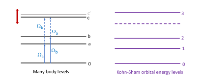
Figure 1: Depiction of a truncated Hilbert space. The true interacting system (left) with three excited states of excitation frequencies $\Omega_{a},\Omega_{b}$ and $\Omega_{c}$, with corresponding KS system (right) with excitation frequencies $\nu_{1},\nu_{2},\nu_{3}$ with 0 being the HOMO level; $\nu_{i}=\epsilon_{i}-\epsilon_{0}$ where $\epsilon_{i}$ is the orbital energy. The possibility of a KS double-excitation of frequency $\nu_{1}+\nu_{2}$ (dashed line) mixing with the single excitation at $\nu_{3}$ yields an additional excitation $\Omega_{c}^{\prime}$ (grey on the left); in this case $c$ and $c^{\prime}$ have both single and double character. Displacement along the red vertical arrow tunes the system out of the resonance condition. In our model, we take the case when $\Omega_{b}=\Omega_{a}$ and $\nu_{2}=\nu_{1}$.

To simplify the inversion, we assume that the KS states have frequencies $\nu_{1},\nu_{3}$ well-separated from each other, and far enough from the ground-state, such that the single-pole approximation may be applied Petersilka et al. (1996); Grabo et al. (2000); Appel et al. (2003); Marques et al. (2012). Then, constructing the linear response functions $\chi$ and $\chi_{\scriptscriptstyle\rm S}$, and the KS quadratic response function $\chi_{\scriptscriptstyle\rm S}^{(2)}$ and using them in Eq. (5)(see Supplemental Material for detail) gives

$$\chi^{(2),{\rm tddft}}_{mnp}(\omega_{1},\omega_{2}) = \left(\frac{a_{c,mi}}{\omega_{1}+\omega_{2}-\Omega_{c}}+\frac{a_{c^{\prime},mi}}{\omega_{1}+\omega_{2}-\Omega_{c^{\prime}}}\right)\left[a_{{\scriptscriptstyle\rm S}3,ij}^{-1}\,\frac{\nu_{1}^{2}}{2\Omega_{a}^{2}}\left(\frac{A_{{\scriptscriptstyle\rm S}13,jnp}}{\omega_{2}-\Omega_{a}}+\frac{A_{{\scriptscriptstyle\rm S}13,jpn}}{\omega_{1}-\Omega_{a}}\right)\right.$$ (6)

$$+ \left.\frac{a_{{\scriptscriptstyle\rm S}3,ij}^{-1}\,\frac{\nu_{1}^{2}}{\Omega_{a}^{2}}\langle f_{\scriptscriptstyle\rm HXC}\rangle_{1}(A_{{\scriptscriptstyle\rm S}13,jnp}+A_{{\scriptscriptstyle\rm S}13,jpn})+g_{{\scriptscriptstyle\rm XC},ijk}(\omega_{1},\omega_{2})a_{a,jn}a_{a,kp}}{(\omega_{2}-\Omega_{a})(\omega_{1}-\Omega_{a})}\right]$$

where $A_{\scriptscriptstyle\rm S13,jnp}=n_{\scriptscriptstyle\rm S01}({\bf r}_{j})n_{\scriptscriptstyle\rm S13}({\bf r}_{n})n_{\scriptscriptstyle\rm S30}({\bf r}_{p})$, $a_{\scriptscriptstyle\rm S3,ij}=n_{\scriptscriptstyle\rm S03}({\bf r}_{i})n_{\scriptscriptstyle\rm S30}({\bf r}_{j})$, defined in terms of the KS transition densities. The residue $a_{c,mi}=n_{0c}({\bf r}_{m})n_{c0}({\bf r}_{i})$ and $\langle f_{\scriptscriptstyle\rm HXC}(\omega_{2})\rangle_{1}=\int\phi_{0}({\bf r})\phi_{1}({\bf r})f_{\scriptscriptstyle\rm HXC}({\bf r},{\bf r}^{\prime},\omega)\phi_{0}({\bf r}^{\prime})\phi_{1}({\bf r}^{\prime})d^{3}{\bf r}d^{3}{\bf r}^{\prime}$. All quantities on the right of Eq. (6) can be obtained from LR TDDFT, the QR kernel, or from the KS system directly.

When $g_{\scriptscriptstyle\rm XC}$ is independent of frequency, the incorrect pole structure is salient, with the last line of Eq. (6) having a three-pole structure instead of the two appearing in the exact $\chi^{(2)}$ of Eq. (4) Parker et al. (2016); Li et al. (2014); Ou et al. (2015a). We note that in most cases the frequencies $\omega_{1,2}$ are in a region dominated by single excitations, where the adiabatic approximation for the linear response xc kernel $f_{\scriptscriptstyle\rm XC}$ does a reasonable job, i.e. the exact $f_{\scriptscriptstyle\rm XC}$ does not have important frequency-dependence in the region it is probed in Eq. (6). Instead, it follows that $g_{\scriptscriptstyle\rm XC}$ must carry a frequency-dependence that removes the extra pole, which means the numerator of the last term in Eq. 6 must be of the form: $X_{inp}(\omega_{1}-\Omega_{a})+Y_{inp}(\omega_{2}-\Omega_{a})$ where $X_{inp}$ and $Y_{inp}$ are functions of $\{{\bf r}_{i},{\bf r}_{n},{\bf r}_{p}\}$. The permutation-symmetry of $\chi^{(2)}$ under $({\bf r}_{1},\omega_{1})\leftrightarrow({\bf r}_{2},\omega_{2})$ implies $Y_{inp}=X_{ipn}$, leading to:

$$X_{inp}(\omega_{1}-\Omega_{a})+X_{ipn}(\omega_{2}-\Omega_{a})=g_{{\scriptscriptstyle\rm XC},ijk}(\omega_{1},\omega_{2})a_{a,jn}a_{a,kp}+a_{{\scriptscriptstyle\rm S}3,ij}^{-1}\,\frac{\nu_{1}^{2}}{\Omega_{a}^{2}}\langle f_{\scriptscriptstyle\rm HXC}(\omega_{2})\rangle_{1}(A_{{\scriptscriptstyle\rm S}13,jnp}+A_{{\scriptscriptstyle\rm S}13,jpn})$$ (7)

Eq. (7) shows that the exact QR kernel $g_{\scriptscriptstyle\rm XC}$ in the vicinity of $\omega_{1,2}$ close to $\Omega_{a}$ has a linear frequency-dependence. For the general case where $\Omega_{a}\neq\Omega_{b}$, a similar analysis leads to $g_{\scriptscriptstyle\rm XC}(\omega_{1}\approx\Omega_{a},\omega_{2}\approx\Omega_{b})$ having a linear behavior as $X(\omega_{1}-\Omega_{a})+Y(\omega_{2}-\Omega_{b})$. It remains now to derive an approximation for $X_{inp}$ which yields a practical approximation for $g_{{\scriptscriptstyle\rm XC},ijk}(\omega_{1},\omega_{2})$.

In order to determine $X_{inp}$, we interpolate between two limiting cases. The first is to set $g_{\scriptscriptstyle\rm XC}\to g_{\scriptscriptstyle\rm XC}^{\rm adia}$ when $\omega_{1}=\omega_{2}=0$ in Eq. (7), which gives an equation for $X_{inp}+X_{ipn}$. A possible solution is

$$X_{inp}=\frac{-1}{2\Omega_{a}}\left(g_{{\scriptscriptstyle\rm XC},ijk}^{\rm adia}a_{a,jn}a_{a,kp}+a_{{\scriptscriptstyle\rm S}3,ij}^{-1}\,\frac{\nu_{1}^{2}}{\Omega_{a}^{2}}\langle f_{\scriptscriptstyle\rm HXC}(\omega_{2})\rangle_{1}A_{{\scriptscriptstyle\rm S}13,jnp}\right)$$ (8)

Using Eq. (8) in Eq. (7) gives $g_{\scriptscriptstyle\rm XC}^{\rm App,1}(\omega_{1},\omega_{2})$ that corrects the single-excitation contribution ($A_{{\scriptscriptstyle\rm S}13,jnp}$ ) to the quadratic response but appears not to include double-excitation contributions to the transition density. It is unclear whether the first term captures true double-excitation character because an adiabatic QR kernel yields a response that has poles at sums of LR-corrected single excitations without any mixing with double-excitations and even these poles are missing when only forward transitions are kept Elliott et al. (2011); Tretiak and Chernyak (2003). Our second limiting case therefore focusses on the double-excitation contribution.

Thus the second limit is the opposite case when state $c$ is a close to a pure double excitation. Considering Fig. 1 the KS state 3 is absent and we denote the KS state with two electrons excited to orbital 1 at the dashed line, as $d$. The KS residue appearing in Eq. (6), $A_{{\scriptscriptstyle\rm S}1d,ijk}=n_{{\scriptscriptstyle\rm S}01}({\bf r}_{i})n_{{\scriptscriptstyle\rm S}1d}({\bf r}_{j})n_{{\scriptscriptstyle\rm S}d0}({\bf r}_{k})=0$ due to the last factor, and equating Eq. (6) to the true $\chi^{(2)}$ in this limit yields

$$a_{c,mi}g^{\rm App,2}_{{\scriptscriptstyle\rm XC},ijk}a_{a,jn}a_{a,kp} = \frac{1}{2}\left[\left(\omega_{1}-\Omega_{a}\right)A_{ca,mnp}\right.$$ (9)

$$+ \left.\left(\omega_{2}-\Omega_{a}\right)A_{ca,mpn}\right]$$

The residue $A_{ca}=n_{0c}n_{ac}n_{a0}$, contains the ground-to-excited transition densities of the true system $n_{0a}$ and $n_{0c}$ which are accessible from LR, and substituting the KS excited-to-excited transition density $n_{1d}$ for $n_{ac}$ in Eq. (9) gives the second limit in our approximation for $g_{\scriptscriptstyle\rm XC}$. Our final approximation interpolates between the two limits through the weighting of the double-excitation component to the true state (details in the Supplemental Material),

$$g_{{\scriptscriptstyle\rm XC},iqr}^{\rm App}(\omega_{1},\omega_{2}) = -\left(\frac{\omega_{1}+\omega_{2}-2\Omega_{a}}{2\Omega_{a}}\right)g_{{\scriptscriptstyle\rm XC},iqr}^{\rm adia}-\left(a_{{\scriptscriptstyle\rm S}3,ij}^{-1}\frac{\nu_{1}^{2}}{\Omega_{a}^{3}}\langle f_{\scriptscriptstyle\rm HXC}(\omega_{2})\rangle_{1}(\omega_{1}A_{{\scriptscriptstyle\rm S}13,jnp}+\omega_{2}A_{{\scriptscriptstyle\rm S}13,jpn})\right.$$

$$+ \left.\frac{a^{-1}_{c,im}}{2}(\sqrt{1-a_{c}a^{-1}_{{\scriptscriptstyle\rm S}3}})_{mo}\frac{n_{0c}(r_{o})}{2}\left[\left(\omega_{1}-\Omega_{a}\right)n_{d1}(r_{n})n_{0a}(r_{p})+\left(\omega_{2}-\Omega_{a}\right)n_{d1}(r_{p})n_{0a}(r_{n})\right]\right)a_{a,nq}^{-1}a_{a,pr}^{-1}$$

For an excited state $c$ that has predominantly single-excitation character, the first two terms dominate, while the third term incorporates the effect of its doubly-excited character. As evident from Eq. (Curing the Divergence in Time-Dependent Density Functional Quadratic Response Theory), all ingredients for our approximation can be obtained from linear response TDDFT, or adiabatic QR TDDFT. Turning to the transition density obtained from the double-residue

$$\xi n_{ca}({\bf r}_{m})=\lim_{\begin{subarray}{c}\omega_{2}\to\Omega_{a}\\ \omega_{1}+\omega_{2}\to\Omega_{c}\end{subarray}}(\omega_{2}-\Omega_{a})(\omega_{1}+\omega_{2}-\Omega_{c})\frac{\chi^{(2)}_{mmm}(\omega_{1},\omega_{2})}{n_{0c}({\bf r}_{m})n_{a0}({\bf r}_{m})}$$ (11)

where $\xi=1$ for the resonant case, and $\xi=\frac{1}{2}$ otherwise, we find

$$n_{ca}^{\rm App}({\bf r})=\sqrt{1-\alpha_{c}^{2}}n_{{\scriptscriptstyle\rm S}1d}({\bf r})+\left(\frac{\nu_{1}}{\Omega_{a}}\right)^{3/2}\alpha_{c}\left(1-2\frac{\langle f_{\scriptscriptstyle\rm HXC}(\omega_{2})\rangle_{1}}{\Omega_{a}}\right)n_{{\scriptscriptstyle\rm S},13}({\bf r})-\frac{n_{0a}({\bf r})}{\Omega_{a}}\int n_{0c}(r_{1})g_{\scriptscriptstyle\rm XC}^{\rm adia}(r_{1},r_{2},r_{3})n_{0a}({\bf r}_{2})n_{0a}({\bf r}_{3})dr_{1}dr_{2}dr_{3}$$ (12)

Here $\alpha_{c}^{2}$ is an ${\bf r}$-independent approximation to $a_{c}a^{-1}_{{\scriptscriptstyle\rm S},3}$: $\alpha_{c}$ ranges from $\sqrt{\nu_{3}/\Omega_{c}}$ in the case where the state $c$ is predominantly a single excitation, to $0$ when it is predominantly a double-excitation. Eq. (12) can be compared with the adiabatic approximation, for which

$$n_{ca}^{\rm adia}({\bf r})=\left(\frac{\nu_{1}}{\Omega_{a}}\right)^{3/2}\alpha_{c}\left(1+\frac{\Omega_{a}-\nu_{1}}{\Omega_{c}-2\Omega_{a}}\right)n_{\scriptscriptstyle\rm S13}({\bf r})+\frac{n_{0a}({\bf r})}{\Omega_{c}-2\Omega_{a}}\int n_{0c}(r_{1})g_{\scriptscriptstyle\rm XC}^{\rm adia}({\bf r}_{1},{\bf r}_{2},{\bf r}_{3})n_{0a}({\bf r}_{2})n_{0a}({\bf r}_{3})dr_{1}dr_{2}dr_{3}\,.$$ (13)

The divergence is evident in the last two terms when the resonant condition, $\Omega_{c}-\Omega_{a}=\Omega_{a}$ is satisfied; further, there is no contribution from any double-excitation.

In practice, there are several ad hoc workarounds to the unphysical divergence, including applying damping factors Aidas et al. (2013), neglecting the kernels in “simplified-TDDFT” Bannwarth and Grimme (2014), setting the term to zero, and the pseudo-wavefunction approximation Li and Liu (2014); Ou et al. (2015b); Alguire et al. (2015); Ou et al. (2015a); Parker et al. (2016) where orbital relaxation terms in the second-order response are neglected, which is equivalent to solving the second-order response equation at zero frequency. The second term in Eq. (12) could be viewed as in the pseudo-wavefunction spirit in the sense that it can be obtained by setting $\omega_{1}$ to zero in the divergent term of Eq. (13). The connections with the standard pseudo-wavefunction approximation are left for future work, including what the implied underlying $g_{\scriptscriptstyle\rm XC}$ kernel is; our work suggests it also has a linear frequency-dependence. In any case, all the standard workarounds miss any double-excitation contribution to the transition density (the first term in Eq. (12)), which can be significant as our first example below demonstrates.

Our first example is a model system of two electrons in a one-dimensional harmonic plus linear potential, $v_{\rm ext}(x)=\frac{1}{2}x^{2}+\gamma|x|$ where $\gamma$ is a parameter in the range$[-1,1]$; varying $\gamma$ tunes the system in and out of the resonance condition. The electrons interact via a soft-Coulomb interaction: $\frac{\lambda}{\sqrt{(x_{1}-x_{2})^{2}+1}}$, where we consider $\lambda=0.2$a.u. as a weak interaction in which the assumptions made in Eqs. (6)–(12) apply, but we also consider the results at the full coupling strength $\lambda=1$a.u. In order to test our approximation for the QR kernel alone, without conflating errors from approximations made to the LR treatment, we will use the exact KS and LR quantities in the equations. The LR thus includes double-excitation contributions, which would be missing in an adiabatic LR treatment.

Fig. 2 shows the transition dipole moment, $\mu_{ac}=\langle\Psi_{a}|\hat{x}|\Psi_{c}\rangle$ between the first two excited states, $\Psi_{a}$ and $\Psi_{c}$ for which the resonance condition, in this case $\Omega_{c}=2\Omega_{a}$, holds as $|\gamma|\rightarrow 0$. We calculate $\alpha_{c}$ from the ratio of the matrix element $\langle\Psi_{0}|\hat{x}^{2}|\Psi_{c}\rangle$ to the corresponding matrix element of the KS system. At the weaker coupling strength $\lambda=0.2$, our approximation Eq. (12) clearly cures the divergence of ALDA shown, and is barely distinguishable from the exact result in quite a wide region around the divergence. Tuning $\gamma$ away from $\gamma=0$, we move away from the resonance condition, and eventually we expect that our approximation may decrease in quality compared to ALDA: the error in our approximation from neglecting the mixing of other single excitations may no longer be negligible compared to the large error caused by the spurious pole in adiabatic approximations in the resonance region. For the particular case here, our approximation continues to do well for positive $\gamma$ where the system remains harmonic at large distances, while for negative values a double-well develops in $v_{\rm ext}$ which brings the two lowest energy levels closer together as delocalized orbitals, deviating from the more clearly separated levels of a single well, and leading to a breakdown of the single-pole-like assumptions in the derivation of Eq. (12). Although our approximation was derived in the limit of well-separated excitations, we still observe a good performance at full coupling strength $\lambda=1.0$ (right panel in Fig. 2), not only curing the divergence seen in ALDA but also giving predictions close to the exact.

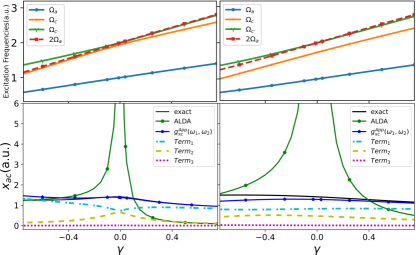
Figure 2: Excitation frequencies (upper) and transition dipole moments (lower panels), $x_{ac}=\langle\Psi_{a}|\hat{x}|\Psi_{c}\rangle$ between the first and 2nd excited states of the model system as a function of parameter, $\gamma$, for $\lambda=0.2$ (left) and $\lambda=1$ (right): exact (black), ALDA (green), our approximation Eq. (12) (blue). The dashed lines term 1, term 2, and term 3 are the respective terms of Eq. (12)

We now turn to LiH, using PBE0 Adamo and Barone (1999) with def2-SVP basis set Weigend and Ahlrichs (2005), within the Turbomole package Balasubramani et al. (2020). The fourth excited state frequency is close to twice the first excited state frequency in the region around 2.6$\AA$ in PBE0; the first and fourth excited states correspond to the first two excited states in the A₁ irreducible representation of $C_{2v}$ point group symmetry. Also around this bond-length, the frequency of the lowest doubly-excited KS state matches that of the 4th single KS excitation (see top right panel Fig. 3). The PBE0 excitation energies are a little shifted from those of the reference full configuration interaction calculation taken from Ref. Parker et al. (2016), while the transition dipole moment diverges in the resonance region $\Omega_{4}=2\Omega_{1}$ Parker et al. (2016). Our approximation, applied together with adiabatic PBE0 LR, shown in Fig. 3 tames this divergence, and follows the trend of the exact result, but with an overestimate; the adiabatic LR lacks the double-excitation contribution which, from the upper right panel could be expected to be significant, and so only the second term in Eq. (12) contributes. Further, we set the third term to zero, because we ran into some numerical problems in its extraction from Turbomole; we note that for the two-electron case of the harmonic oscillator where $g_{\scriptscriptstyle\rm X}^{\rm adia}$ is strictly zero and $g_{\scriptscriptstyle\rm C}^{adia}$ was small, it may be small in this case as well. Likely, including this together with the double-excitation contribution with the LR kernel of Ref. Maitra et al. (2004) should improve the performance of our QR kernel; we leave for future work the investigation of oscillator strengths from a modified dressed LR TDDFT Mazur and Włodarczyk (2009); Casida (1995); Carrascal et al. (2018) which would be used to determine $\alpha_{c}$. The figure shows also the result from the pseudo-wavefunction approximation that is often used Parker et al. (2016); Alguire et al. (2015); Ou et al. (2015a), which, despite being an ad hoc correction, appears to perform a little better than ours on when compared with the same relative position in FCI. Again, as we move away from the resonance region, our approximation deviates as expected; the prescription would be that we revert to adiabatic PBE0 when the curves meet.

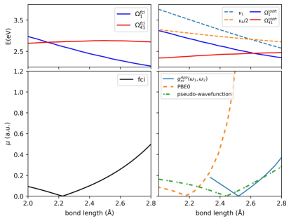
Figure 3: Upper panel: (left) Full configuration interaction (fci) and (right) TDDFT frequencies between the ground and the first excited state (solid blue), and the first and fourth excited state of LiH, $\Omega_{41}=\Omega_{4}-\Omega_{1}$(solid red). The right panel also shows the KS lowest transition frequency, $\nu_{1}$ (light blue dotted ) and half of the fourth KS frequency, $\nu_{4}$ (orange dotted). Lower panel: Transition dipole moment, $\mu_{14}$ between the first and fourth excited states as a function of bond-length; exact (black), our approximation Eq. (12)(light blue), PBE0 (orange dashed), and pseudo-wavefunction approximation (green dashed). Note that for bond-lengths greater than $2.4\AA$ the adiabatic PBE0 is out of the scale of the figure.

In summary, we found the form of the exact frequency-dependent kernel in QR TDDFT and derived an approximate kernel based on this. Tests on the excited-state transition amplitudes of a model system and on the LiH molecule suggest it is a promising practical cure to the unphysical divergence problem in adiabatic QR TDDFT; Eq. (Curing the Divergence in Time-Dependent Density Functional Quadratic Response Theory) can be applied also to cure the divergences in other second-order response properties such as hyperpolarizabilities, two-photon absorption, etc. Our approach can be generalized to situations beyond the single-pole-type of analysis here, when more than one KS single-excitation contributes to a given state. Alternatives to the two limiting approximations that we interpolated between here may lead to improved accuracy and will be explored in future work. This work also stresses the importance of including double-excitation contributions in LR; the kernel of Ref. Maitra et al. (2004) needs to be generalized to describe how the oscillator strength gets redistributed in this case Casida (1995); Mazur and Włodarczyk (2009); Carrascal et al. (2018). We note that TDDFT can also be applied in the real-time domain to obtain non-linear optical properties Cocchi et al. (2014) and the implications of the frequency-domain divergences for the time-domain have yet to be explored. Future work also includes determining whether the divergence is related to the spurious pole shift of generalized LR TDDFT Fuks et al. (2015); Luo et al. (2016); Maitra (2016) in the adiabatic approximation, as was previously surmised Parker et al. (2016). The QR kernel is the functional derivative, or response, of the LR kernel evaluated at the ground-state, and in this sense may be viewed as containing information about the linear response of an excited state. On the other hand, the pole shifting occurs quite generally, not just in situations where the resonance condition is satisfied.

I Supporting Information

Detailed derivations and discussion of Eq (6) and the steps in the approximation leading to Eq. (10).

I.1 (I) Derivation of the TDDFT Second Order Response Equation in the Truncated Hilbert Space

The Dyson equation for the second-order response function was derived in Ref. Gross et al. (1996) in terms of the linear response xc kernel, the KS response function, and the quadratic response xc kernel. (We note a typo in Eq. (173) of Ref. Gross et al. (1996) where the step functions on the right should read $\theta(t-\tau)\theta(\tau-\tau^{\prime})$). To transform the time-domain expression into the frequency-domain, we Fourier transform using the factors $e^{i\omega_{1}(t-t_{1})}e^{i\omega_{1}(t-t_{2})}$ Elliott et al. (2011). Combining the resulting equation with the Dyson equation in linear response, we obtain

$$\chi_{mnp}^{(2),{\rm tddft}}(\omega_{1},\omega_{2}) = \chi_{mi}(\omega_{1}+\omega_{2})\chi_{{\scriptscriptstyle\rm S},ij}^{-1}(\omega_{1}+\omega_{2})\chi_{{\scriptscriptstyle\rm S},jkl}^{(2)}(\omega_{1},\omega_{2})\chi_{{\scriptscriptstyle\rm S},lq}^{-1}(\omega_{1})\chi_{qn}(\omega_{1})\chi_{{\scriptscriptstyle\rm S},kr}^{-1}(\omega_{2})\chi_{rp}(\omega_{2})$$ (S.14)

$$+ \chi_{mi}(\omega_{1}+\omega_{2})g_{{\scriptscriptstyle\rm XC},ijk}(\omega_{1},\omega_{2})\chi_{jn}(\omega_{1})\chi_{kp}(\omega_{2})\,,$$

where, as in the main text, the subscripts represent the spatial variables.

We will evaluate the terms explicitly within the assumption of the truncated subspace discussed in the main text. The frequencies $\omega_{1},\omega_{2}$ are taken to be far closer to $\Omega_{a}$ than to $\Omega_{c}$, while their sum $\omega_{1}+\omega_{2}$ is far closer to $\Omega_{c}$ than to $\Omega_{a}$. Further, we make a single-pole (Tamm-Dancoff)-like approximation in that we neglect the backward transitions, but we restore the oscillator strength sum-rule when relating the transition amplitudes of the KS and interacting systems.

With these considerations, we find the first-order response functions:

$$\chi_{ij}(\omega_{1(2)})\approx\frac{a_{a,ij}}{\omega_{1(2)}-\Omega_{a}}\;\;\;{\rm where}\;\;\;a_{a,ij}=n_{0a}({\bf r}_{i})n_{a0}({\bf r}_{j}),\;\;\;{\rm with}\;\;\;n_{0a}({\bf r})=\langle\Psi_{0}|\hat{n}({\bf r})|\Psi_{a}\rangle$$ (S.15)

$$\chi_{{\scriptscriptstyle\rm S},ij}(\omega_{1(2)})\approx\frac{a_{{\scriptscriptstyle\rm S}1,ij}}{\omega_{1(2)}-\nu_{1}},\;\;\;{\rm where}\;\;\;a_{{\scriptscriptstyle\rm S}1,ij}=n_{{\scriptscriptstyle\rm S}01}({\bf r}_{i})n_{{\scriptscriptstyle\rm S}10}({\bf r}_{j})$$

where the subscript ${\scriptscriptstyle\rm S}$ indicates KS quantities, and similarly,

$$\chi_{ij}(\omega_{1}+\omega_{2})\approx\frac{a_{c,ij}}{\omega_{1}+\omega_{2}-\Omega_{c}}+\frac{a_{c^{\prime},ij}}{\omega_{1}+\omega_{2}-\Omega_{c^{\prime}}}$$ (S.17)

$$\chi_{{\scriptscriptstyle\rm S}ij}(\omega_{1}+\omega_{2})\approx\frac{a_{{\scriptscriptstyle\rm S3},ij}}{\omega_{1}+\omega_{2}-\nu_{3}}$$ (S.18)

For the second order KS response function we have

$$\chi^{(2)}_{{\scriptscriptstyle\rm S},jkl}(\omega_{1},\omega_{2})\approx\frac{1}{2}\left(\frac{A_{{\scriptscriptstyle\rm S}13,jkl}}{(\omega_{1}+\omega_{2}-\nu_{3})(\omega_{2}-\nu_{1})}+\frac{A_{{\scriptscriptstyle\rm S}13,jlk}}{(\omega_{1}+\omega_{2}-\nu_{3})(\omega_{1}-\nu_{1})}\right)$$ (S.19)

We make use of the single-pole approximation

$$\Omega_{a}=\nu_{1}+2\langle f_{\scriptscriptstyle\rm HXC}\rangle_{1}\;\;{\rm where}\;\;\langle f_{\scriptscriptstyle\rm HXC}\rangle_{1}\equiv\int d{\bf r}d{\bf r}^{\prime}\phi_{0}({\bf r})\phi_{1}({\bf r})f_{\scriptscriptstyle\rm HXC}({\bf r},{\bf r}^{\prime},\omega)\phi_{0}({\bf r}^{\prime})\phi_{1}({\bf r}^{\prime})$$ (S.20)

and impose the oscillator strength sum rule within the single-excitation approximation

$$\Omega_{a}a_{a}\approx\nu_{1}a_{{\scriptscriptstyle\rm S1}}$$ (S.21)

to express

$$\chi_{{\scriptscriptstyle\rm S},kr}^{-1}(\omega_{2})\chi_{rp}(\omega_{2})\approx\frac{\omega_{2}-\nu_{1}}{\omega_{2}-\Omega_{a}}\frac{\nu_{1}}{\Omega_{a}}\delta_{kp}$$ (S.22)

We note that making use of the single-pole approximation includes a diagonal correction to the KS excitation frequency and neglects coupling of the single-excitation to other single-excitations through off-diagonal elements of the kernel; this is justified by the stated assumption that the KS orbital energies are well-separated. This assumption could be relaxed however, at the cost of a more complicated expression for the kernel; this would be in the same spirit as was done in a different context, Ref. Cave et al. (2004), when applying the dressed TDDFT kernel to double-excitations in linear polyenes, for example. Since the residues of the response functions are of central interest in this work, we wish to respect and restore the oscillator strength sum-rule as above Casida (1995); Grabo et al. (2000); Appel et al. (2003).

Putting these together we finally obtain

$$\chi^{(2),{\rm tddft}}_{mnp}(\omega_{1},\omega_{2}) = \left(\frac{a_{c,mi}}{\omega_{1}+\omega_{2}-\Omega_{c}}+\frac{a_{c^{\prime},mi}}{\omega_{1}+\omega_{2}-\Omega_{c^{\prime}}}\right)\left[a_{{\scriptscriptstyle\rm S}3,ij}^{-1}\,\frac{\nu_{1}^{2}}{2\Omega_{a}^{2}}\left(\frac{A_{{\scriptscriptstyle\rm S}13,jnp}}{\omega_{2}-\Omega_{a}}+\frac{A_{{\scriptscriptstyle\rm S}13,jpn}}{\omega_{1}-\Omega_{a}}\right)\right.$$ (S.23)

$$+ \left.\frac{a_{{\scriptscriptstyle\rm S}3,ij}^{-1}\,\frac{\nu_{1}^{2}}{\Omega_{a}^{2}}\langle f_{\scriptscriptstyle\rm HXC}\rangle_{1}(A_{{\scriptscriptstyle\rm S}13,jnp}+A_{{\scriptscriptstyle\rm S}13,jpn})+g_{{\scriptscriptstyle\rm XC},ijk}(\omega_{1},\omega_{2})a_{a,jn}a_{a,kp}}{(\omega_{2}-\Omega_{a})(\omega_{1}-\Omega_{a})}\right]$$

which is Eq. (6) in the main paper.

I.2 (II) Approximation for the QR Kernel

As observed in the paper, an adiabatic approximation for $g_{\scriptscriptstyle\rm XC}(\omega_{1},\omega_{2})$ leaves the expression for $\chi^{(2),{\rm tddft}}$ with an excess pole compared to the exact $\chi^{(2)}$, which is ultimately responsible for the divergence in the residues. An approximation for $g_{\scriptscriptstyle\rm XC}$ must have a frequency dependence that removes this pole which means the numerator of the last term of Eq. (S.23) above must be of the form:

$$X_{inp}(\omega_{1}-\Omega_{a})+Y_{ipn}(\omega_{2}-\Omega_{a})$$ (S.24)

Considering the symmetry of $\chi^{(2)}$ under $({\bf r}_{n},{\bf r}_{p},\omega_{1})\leftrightarrow({\bf r}_{p},{\bf r}_{n},\omega_{2})$, we deduce that $Y_{ipn}=X_{ipn}$, and so the approximation for $g_{\scriptscriptstyle\rm XC}(\omega_{1},\omega_{2})$ reduces to finding an approximation for $X_{inp}$. Equating the numerator of the last term of Eq. (S.23) to Eq. (S.24) with $Y_{ipn}=X_{ipn}$, gives Eq. (7) in the main text.

As discussed in the main paper, our approximation is derived from two limiting cases for which we provide more detail here.

(i) First limiting case: We set $g_{\scriptscriptstyle\rm XC}\rightarrow g_{\scriptscriptstyle\rm XC}^{\rm adia}$ when $\omega_{1}=\omega_{2}=0$ in Eq (7) of the main text, which gives Eq. 8 of the main text for $X_{inp}$. Such an approximation leads to the QR kernel

$$g_{{\scriptscriptstyle\rm XC},iqr}^{\rm App-1}(\omega_{1},\omega_{2})=-\left(\frac{\omega_{1}+\omega_{2}-2\Omega_{a}}{2\Omega_{a}}\right)g_{{\scriptscriptstyle\rm XC},iqr}^{\rm adia}-a_{{\scriptscriptstyle\rm S}3,ij}^{-1}\frac{\nu_{1}^{2}}{\Omega_{a}^{3}}\langle f_{\scriptscriptstyle\rm HXC}(\omega_{2})\rangle_{1}(\omega_{1}A_{{\scriptscriptstyle\rm S}13,jnp}+\omega_{2}A_{{\scriptscriptstyle\rm S}13,jpn})a_{a,nq}^{-1}a_{a,pr}^{-1}$$ (S.25)

which, when inserted into Eq.(6), gives

$$\chi^{(2),{\rm App-1}}_{mnp}(\omega_{1},\omega_{2}) = \left(\frac{a_{c,mi}}{\omega_{1}+\omega_{2}-\Omega_{c}}+\frac{a_{c^{\prime},mi}}{\omega_{1}+\omega_{2}-\Omega_{c^{\prime}}}\right)\left[a_{{\scriptscriptstyle\rm S}3,ij}^{-1}\,\frac{\nu_{1}^{2}}{2\Omega_{a}^{2}}\left(\frac{A_{{\scriptscriptstyle\rm S}13,jnp}}{\omega_{2}-\Omega_{a}}+\frac{A_{{\scriptscriptstyle\rm S}13,jpn}}{\omega_{1}-\Omega_{a}}\right)\left(1-\frac{2\langle f_{\scriptscriptstyle\rm HXC}(\omega_{2})\rangle_{1}}{\Omega_{a}}\right)\right.$$ (S.26)

$$- \left.\frac{1}{2\Omega_{a}}\left(\frac{1}{\omega_{1}-\Omega_{a}}+\frac{1}{\omega_{2}-\Omega_{a}}\right)g_{{\scriptscriptstyle\rm XC},ijk}^{\rm adia}a_{a,jn}a_{a,kp}\right]$$

If we were then to extract the transition density between states $a$ and $c$ (Eq. 11 of the main text), we obtain

$$n_{ca}^{\rm App-1}({\bf r})=\left(\frac{\nu_{1}}{\Omega_{a}}\right)^{3/2}\left(1-2\frac{\langle f_{\scriptscriptstyle\rm HXC}\rangle_{1}}{\Omega_{a}}\right)\alpha_{c}n_{{\scriptscriptstyle\rm S},13}({\bf r})-\frac{n_{0a}({\bf r})}{\Omega_{a}}\int n_{0c}({\bf r}_{1})g_{\scriptscriptstyle\rm XC}^{\rm adia}(r_{1},r_{2},r_{3})n_{0a}({\bf r}_{2})n_{0a}({\bf r}_{3})d{\bf r}_{1}d{\bf r}_{2}d{\bf r}_{3}$$ (S.27)

where we have defined $\alpha_{c}^{2}$ as an ${\bf r}$-independent approximation to $a_{c,ij}a^{-1}_{{\scriptscriptstyle\rm S}3,jk}$:

$$a_{c}\approx\alpha_{c}^{2}a_{{\scriptscriptstyle\rm S}3}$$ (S.28)

Physically, $\alpha_{c}$ reflects the ratio of the true transition density to the KS one. Due to the oscillator-strength sum-rule applied within the separated levels assumption, $\alpha_{c}^{2}\approx\nu_{3}/\Omega_{c}$ when the interacting state is predominantly a single-excitation. When there is mixing with a KS double-excitation however, $\alpha_{c}^{2}$ decreases, reducing to zero in the limit of a pure double-excitation. This approximation (Eq. (S.27)) however appears not to include double-excitation contributions to the transition density. The first term corrects the single-excitation component, while it is unclear whether the second term, which tends to be much smaller than the first, captures true double-excitation character: an adiabatic QR kernel yields a response that has poles at sums of LR-corrected single excitations without any mixing with double-excitations but even these poles are missing when only forward transitions are kept Elliott et al. (2011). Our second limiting case therefore focusses on the double-excitation contribution.

(ii) Second limiting case: Here we consider the case when state $c$ is close to a pure double-excitation of the KS system, denoted $d$. There is no single KS excitation in the vicinity, so no pole in the KS LR function nearby. This means that the KS residue $A_{{\scriptscriptstyle\rm S}1d,ijk}=n_{01}({\bf r}_{i})n_{1d}({\bf r}_{j})n_{d0}({\bf r}_{k})$ is strictly zero because $n_{d0}({\bf r})\equiv 0$ since a one-body operator cannot connect determinants different by two orbitals. The interacting residue is small but non-zero because the corresponding term $n_{c0}$ involves the state $c$ which has small contributions from single-excitations to the KS double excitation that dominates the interacting state in this limit. In this limit the exact interacting $\chi^{(2)}$ has the form

$$\chi^{(2)}_{mnp}(\omega_{1},\omega_{2})=\frac{1}{2(\omega_{1}+\omega_{2}-\Omega_{c})}\left(\frac{A_{ca,mnp}}{\omega_{2}-\Omega_{a}}+\frac{A_{ca,mpn}}{\omega_{1}-\Omega_{a}}\right),\;\;\;A_{ca}=n_{0c}n_{ca}n_{a0}$$ (S.29)

so that equating Eq. (S.23) to this, gives Eq. (9) of the main paper. We now approximate the part of the residue $A_{ca}$ that is not accessible from LR, $n_{ca}$ simply by the KS transition-density $n_{d1}$, yielding

$$a_{c,mi}g^{\rm App-2}_{{\scriptscriptstyle\rm XC},ijk}a_{a,jn}a_{a,kp}=\frac{n_{0c}({\bf r}_{m})}{2}\left[\left(\omega_{1}-\Omega_{a}\right)n_{d1}({\bf r}_{n})n_{0a}({\bf r}_{p})+\left(\omega_{2}-\Omega_{a}\right)n_{d1}({\bf r}_{p})n_{0a}({\bf r}_{n})\right]$$ (S.30)

Our complete approximation interpolates between limits (1) and (2) through

$$g_{\scriptscriptstyle\rm XC}^{\rm App}=g_{\scriptscriptstyle\rm XC}^{\rm App-1}+\sqrt{1-a_{c}a^{-1}_{{\scriptscriptstyle\rm S}3}}g_{\scriptscriptstyle\rm XC}^{\rm App-2}$$ (S.31)

as in Eq. (10) of the main text, with the rationale that $1-a_{c}a^{-1}_{{\scriptscriptstyle\rm S}3}$ represents the fraction of the true oscillator strength arising from the double-excitation component of the state.

References

- Papadopoulos et al. (2006) M. G. Papadopoulos, A. J. Sadlej, and J. Leszczynski, eds., Non-Linear Optical Properties of Matter (Springer Netherlands, 2006).
- Mukamel (1999) S. Mukamel, Principles of Non-Linear Optical Spectroscopy (Oxford University Press, 1999).
- Parker et al. (2016) S. M. Parker, S. Roy, and F. Furche, Journal of chemical physics 145, 134105 (2016).
- Dalgaard (1982) E. Dalgaard, Phys. Rev. A 26, 42 (1982).
- Li and Liu (2014) Z. Li and W. Liu, The Journal of Chemical Physics 141, 014110 (2014).
- Ou et al. (2015a) Q. Ou, G. D. Bellchambers, F. Furche, and J. E. Subotnik, The Journal of chemical physics 142, 064114 (2015a).
- Zhang and Herbert (2015) X. Zhang and J. M. Herbert, The Journal of Chemical Physics 142, 064109 (2015).
- Runge and Gross (1984) E. Runge and E. K. U. Gross, Phys. Rev. Lett. 52, 997 (1984).
- Ullrich (2011) C. A. Ullrich, Time-dependent density-functional theory: concepts and applications (Oxford University Press, 2011).
- Marques et al. (2012) M. A. Marques, N. T. Maitra, F. M. Nogueira, E. K. Gross, and A. Rubio, eds., Fundamentals of time-dependent density functional theory, Vol. 837 (Springer, 2012).
- Maitra (2016) N. T. Maitra, The Journal of Chemical Physics 144, 220901 (2016).
- Gross et al. (1996) E. K. U. Gross, J. F. Dobson, and M. Petersilka, in Density Functional Theory II: Relativistic and Time Dependent Extensions, edited by R. F. Nalewajski (Springer Berlin Heidelberg, Berlin, Heidelberg, 1996) pp. 81–172.
- Petersilka et al. (1996) M. Petersilka, U. J. Gossmann, and E. K. U. Gross, Phys. Rev. Lett. 76, 1212 (1996).
- Casida (1995) M. Casida, in Recent Advances in Density Functional Methods, Part I, edited by D. Chong (World Scientific, Singapore, 1995).
- Maitra et al. (2004) N. T. Maitra, F. Zhang, R. J. Cave, and K. Burke, The Journal of Chemical Physics 120, 5932 (2004).
- Maitra (2022) N. T. Maitra, Annual Review of Physical Chemistry 73, 117 (2022).
- Wehrum and Hermeking (1974) R. P. Wehrum and H. Hermeking, Journal of Physics C: Solid State Physics 7, L107 (1974).
- Senatore and Subbaswamy (1987) G. Senatore and K. Subbaswamy, Physical Review A 35, 2440 (1987).
- Parker and Furche (2018) S. M. Parker and F. Furche, “Response theory and molecular properties,” in Frontiers of Quantum Chemistry, edited by M. J. Wójcik, H. Nakatsuji, B. Kirtman, and Y. Ozaki (Springer Singapore, Singapore, 2018) pp. 69–86.
- Sałek et al. (2002) P. Sałek, O. Vahtras, T. Helgaker, and H. Ågren, The Journal of chemical physics 117, 9630 (2002).
- Aidas et al. (2013) K. Aidas, C. Angeli, K. L. Bak, V. Bakken, R. Bast, L. Boman, O. Christiansen, R. Cimiraglia, S. Coriani, P. Dahle, E. K. Dalskov, U. Ekström, T. Enevoldsen, J. J. Eriksen, P. Ettenhuber, B. Fernández, L. Ferrighi, H. Fliegl, L. Frediani, K. Hald, A. Halkier, C. Hättig, H. Heiberg, T. Helgaker, A. C. Hennum, H. Hettema, E. Hjertenaes, S. Høst, I.-M. Høyvik, M. F. Iozzi, B. Jansík, H. J. A. Jensen, D. Jonsson, P. Jørgensen, J. Kauczor, S. Kirpekar, T. Kjaergaard, W. Klopper, S. Knecht, R. Kobayashi, H. Koch, J. Kongsted, A. Krapp, K. Kristensen, A. Ligabue, O. B. Lutnaes, J. I. Melo, K. V. Mikkelsen, R. H. Myhre, C. Neiss, C. B. Nielsen, P. Norman, J. Olsen, J. M. H. Olsen, A. Osted, M. J. Packer, F. Pawlowski, T. B. Pedersen, P. F. Provasi, S. Reine, Z. Rinkevicius, T. A. Ruden, K. Ruud, V. V. Rybkin, P. Sałek, C. C. M. Samson, A. S. de Merás, T. Saue, S. P. A. Sauer, B. Schimmelpfennig, K. Sneskov, A. H. Steindal, K. O. Sylvester-Hvid, P. R. Taylor, A. M. Teale, E. I. Tellgren, D. P. Tew, A. J. Thorvaldsen, L. Thøgersen, O. Vahtras, M. A. Watson, D. J. D. Wilson, M. Ziolkowski, and H. Ågren, Wiley Interdisciplinary Reviews: Computational Molecular Science 4, 269 (2013).
- Balasubramani et al. (2020) S. G. Balasubramani, G. P. Chen, S. Coriani, M. Diedenhofen, M. S. Frank, Y. J. Franzke, F. Furche, R. Grotjahn, M. E. Harding, C. Hättig, A. Hellweg, B. Helmich-Paris, C. Holzer, U. Huniar, M. Kaupp, A. Marefat Khah, S. Karbalaei Khani, T. Müller, F. Mack, B. D. Nguyen, S. M. Parker, E. Perlt, D. Rappoport, K. Reiter, S. Roy, M. Rückert, G. Schmitz, M. Sierka, E. Tapavicza, D. P. Tew, C. van Wüllen, V. K. Voora, F. Weigend, A. Wodyński, and J. M. Yu, J. Chem. Phys. 152, 184107 (2020).
- Gonze and Vigneron (1989) X. Gonze and J.-P. Vigneron, Phys. Rev. B 39, 13120 (1989).
- Van Gisbergen et al. (1997) S. Van Gisbergen, J. Snijders, and E. Baerends, Physical review letters 78, 3097 (1997).
- Zhu et al. (2021) H. Zhu, J. Wang, F. Wang, E. Feng, and X. Sheng, Chemical Physics Letters 785, 139150 (2021).
- Norman et al. (2005) P. Norman, D. M. Bishop, H. J. A. Jensen, and J. Oddershede, The Journal of chemical physics 123, 194103 (2005).
- Kjaegaard et al. (2008) T. Kjaegaard, P. Jorgensen, J. Olsen, S. Coriani, and T. Helgaker, The Journal of Chemical Physics 129, 054106 (2008), https://doi.org/10.1063/1.2961039 .
- Zahariev and Gordon (2014) F. Zahariev and M. S. Gordon, The Journal of Chemical Physics 140, 18A523 (2014).
- Hu et al. (2016) Z. Hu, J. Autschbach, and L. Jensen, Journal of Chemical Theory and Computation 12, 1294 (2016).
- Li et al. (2014) Z. Li, B. Suo, and W. Liu, The Journal of chemical physics 141, 244105 (2014).
- Grabo et al. (2000) T. Grabo, M. Petersilka, and E. Gross, Journal of Molecular Structure: THEOCHEM 501, 353 (2000).
- Appel et al. (2003) H. Appel, E. K. Gross, and K. Burke, Physical review letters 90, 043005 (2003).
- Elliott et al. (2011) P. Elliott, S. Goldson, C. Canahui, and N. T. Maitra, Chem. Phys. 391, 110 (2011).
- Tretiak and Chernyak (2003) S. Tretiak and V. Chernyak, The Journal of Chemical Physics 119, 8809 (2003), http://dx.doi.org/10.1063/1.1614240 .
- Bannwarth and Grimme (2014) C. Bannwarth and S. Grimme, Computational and Theoretical Chemistry 1040-1041, 45 (2014).
- Ou et al. (2015b) Q. Ou, E. C. Alguire, and J. E. Subotnik, The Journal of Physical Chemistry B 119, 7150 (2015b).
- Alguire et al. (2015) E. C. Alguire, Q. Ou, and J. E. Subotnik, The Journal of Physical Chemistry B 119, 7140 (2015).
- Adamo and Barone (1999) C. Adamo and V. Barone, J. Chem. Phys. 110, 6158 (1999).
- Weigend and Ahlrichs (2005) F. Weigend and R. Ahlrichs, Physical Chemistry Chemical Physics 7, 3297 (2005).
- Mazur and Włodarczyk (2009) G. Mazur and R. Włodarczyk, J. Comput. Chem. 30, 811 (2009).
- Carrascal et al. (2018) D. J. Carrascal, J. Ferrer, N. Maitra, and K. Burke, The European Physical Journal B 91, 142 (2018).
- Cocchi et al. (2014) C. Cocchi, D. Prezzi, A. Ruini, E. Molinari, and C. A. Rozzi, Phys. Rev. Lett. 112, 198303 (2014).
- Fuks et al. (2015) J. I. Fuks, K. Luo, E. D. Sandoval, and N. T. Maitra, Phys. Rev. Lett. 114, 183002 (2015).
- Luo et al. (2016) K. Luo, J. I. Fuks, and N. T. Maitra, The Journal of Chemical Physics 145, 044101 (2016).
- Cave et al. (2004) R. J. Cave, F. Zhang, N. T. Maitra, and K. Burke, Chemical Physics Letters 389, 39 (2004).