Non-Hermitian topological invariant of photonic band structures undergoing inversion

Abstract

The interplay between symmetry and topology led to the discovery of symmetry-protected topological phases in Hermitian systems, including topological insulators and topological superconductors. However, the intrinsic symmetry-protected topological characteristics of non-Hermitian systems still await exploration. Here, we investigate experimentally the topological transition associated with the inversion of non-Hermitian band structures in an optical lattice. Intriguingly, we demonstrate that the winding number associated with the symmetry-protected bound state in the continuum is not a conserved quantity after band inversion. To define a topological invariant, we propose the skyrmion number given by spawning in momentum space a pseudo-spin with the polarisation vortex as the in-plane component and the band-index as the pseudo-spin direction at the origin. This leads to a topological transition from an antimeron to an meron-like texture through band inversion, while always conserving the half-charge skyrmion number. We foresee the use of skyrmion number to explore exotic singularities in various non-Hermitian physical system.

In 1929, Von Neumann and Wigner suggested, as an anecdote, the existence of peculiar solutions of Schrödinger equation which are perfect bound states although lying in the continuum spectrum of extended states [1]. Six decades later, the origin of Bound States in the Continuum (BICs) was elegantly unraveled in 1985 by Friedrich and Wintgen, who explained the suppression of the leaking to the continuum as the result of destructive interference between two resonances when coupled to the same radiation channel [2]. Nowadays, BICs have been evidenced in many physical platform, such as atomic and molecular system [3, 4, 5], water waves [6], solid-state and mesoscopic physics [7, 8, 9], and photonic structures [10, 11]. In particular, engineering BICs with custom-cut design in nanophotonics has led to tremendous success in various applications such as lasing[11, 12], ultra-fast optical switch[13] and sensing[14, 15].

The seminal work of Zhen et al.[16] has shown that each BIC in photonic lattices corresponds to a polarization singularity associated with a polarization vortex in momentum space. These vectorial vortices have now been experimentally demonstrated by different groups[17, 18]. Ultimately, the winding number of such a polarization vortex is suggested to be a conserved topological charge of non-Hermitian photonics[16, 19]. This interpretation is now widely accepted since the winding number has been theoretically and experimentally demonstrated as a conserved quantity in different scenarios such as BIC merging, splitting, annihilation, and creation[16, 20, 21, 22, 23, 24]. Most of these works have focused on mechanisms either involving accidental BICs[16, 20, 23], or breaking lattice symmetry[21, 22].

However, symmetries play a crucial role in classifying topological phases of matters [25, 26] as well as in interpreting topological photonics systems [27]. On the other hand, the topological order can be altered with the band inversion mechanism while preserving the symmetries [28, 29]. Therefore investigating the topological nature of photonic symmetry-protected BICs under band inversion mechanism is fundamentally important.

In this work, we experimentally investigate the topological nature of symmetry-protected BICs undergoing band inversion transformation in leaky photonic lattice. Using a home-built band dispersion tomography setup, we map the polarization texture in momentum space together with the dispersion surface of each photonic band. Our results show that the polarization vortex associated with the symmetry-protected BIC changes sign after the band inversion. The results suggest that the winding number is not a good topological number as soon as the band inversion mechanism is involved. We then propose the definition of skyrmion number [30, 31] for non-Hermitian topological charges, which combines the winding number of symmetry-protected BICs and their band index. The latter can be interpreted as the direction of the pseudo-spin at the origin, leading to a meron-like texture in the momentum space.

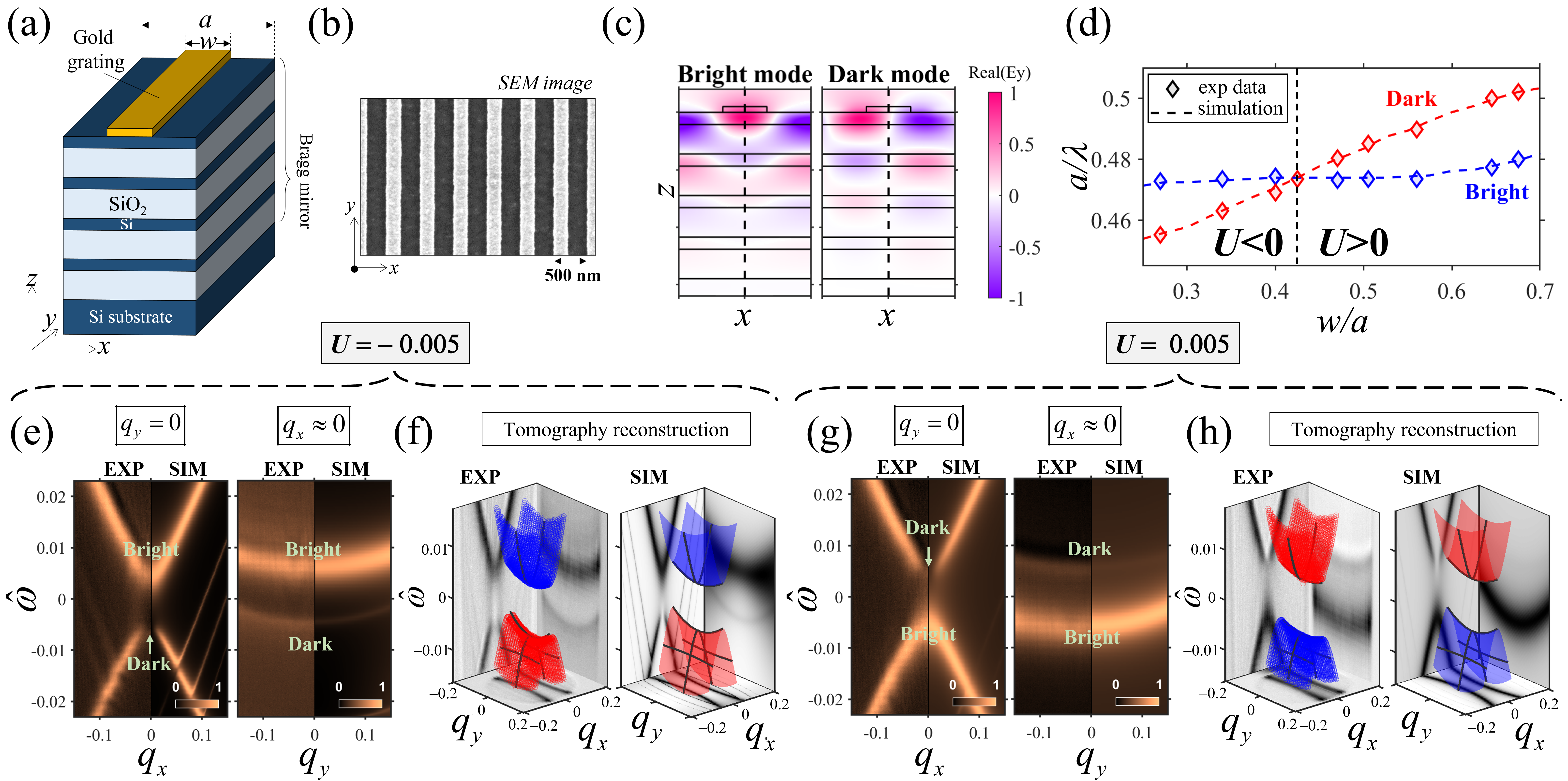
Figure 1: (a) Sketch of the sample: photonic lattices consisting of gold gratings of period $a=600\,$nm and $50\,$nm thickness, on top of a dielectric mirror (4 pairs of $SiO_{2}/Si$ Bragg mirror). The width $w$ of gold stripes is in the range of $0.25a$ to $0.7a$. (b) Top view of a Scanning Electronic Microscope (SEM) image of the sample. (c) Field distribution of lowest energy eigenmodes at normal incidence (i.e. $k_{x}=k_{y}=0$). (d) Energy (in the unit of $a/\lambda$) of the eigenmodes as a function of the aspect ratio $w/a$. The open diamond symbols are experimental data and the dash lines are results obtained from RCWA simulations. (e,g) Band structure of the photonic lattice in the case of (e) $U<0$ and (g) $U>0$ experimentally measured by angle-resolved reflectivity contrast (left panels), and numerically simulated by RCWA method (right panels). These band structures are depicted along $q_{x}$ (with $q_{y}=0$) and along $q_{y}$ (with $q_{x}\approx 0$). Here $q_{x}=k_{x}.a/2\pi$ and $q_{y}=k_{y}.a/2\pi$, and the energy axis is the normalized pulsation, given by $\hat{\omega}=(\omega-\omega_{0})a/2\pi c$ where $\omega_{0}$ is the mid-gap frequency. (f,h) Tomography of the dispersion surface in the case of (f) $U<0$ and (h) $U>0$ reconstructed from band structure measurements (left panels) and RCWA simulations (right panels).

Figure 2: (a to d) Mapping of the farfield polarization orientation $\phi$ in momentum space $(q_{x},q_{y})$ from respectively (a) the upper and (b) lower branch before the band inversion; (c) the upper and (d) lower branch after the band inversion. The farfield polarization maps are reconstructed from (i) experimental data, (ii) Finite Element Method (FEM) simulations, and effective Hamiltonian ((iii) colormap , (iv) vectorial representation).

The photonic lattice that we examine, shown in Figs.1(a,b), consists of a thin metal sub-wavelength grating on top of a dielectric mirror (the structure is periodically modulated along $x$-axis and invariant by translation along $y$-axis). Such designs have been considered in previous works as Tamm plasmon photonic crystals[32], but here we refer to it simply as a case study of photonic lattices. Indeed, most of the results in this work should be reproduced in any other sub-wavelength photonic lattice exhibiting an in-plane mirror symmetry along the corrugation direction $x\rightarrow-x$ and translational invariance in the $y$ direction. In this work, we will focus on Transverse Electric (TE) modes, keeping in mind that similar effects would be obtained for Transverse Magnetic (TM) modes (the only condition is that the splitting TE-TM is strong enough so that there is single polarization mode at the operating frequency). At the $\Gamma$ point, the two lowest TE eigenmodes exhibit opposite parity with respect to the in-plan mirror symmetry, as seen in Fig.1(c). The antisymmetric mode is not allowed to couple to plane waves of the radiative continuum, thus corresponding to a symmetry-protected BIC. On the other hand, the symmetric mode can radiate to the free space. Due to the presence of nonradiative losses via absorption in metal, both modes have a finite quality factor. Since some papers only use the term BIC when the quality factor is infinite (and quasi-BIC or ultrahigh-Q otherwise), to avoid any misleading, for the rest of the paper, the symmetry-protected BIC will be referred to as the dark mode, while the radiative eigenmode will be referred to as the bright mode.

For an arbitrary point in momentum space in the vicinity of the $\Gamma$ point, the formation of these eigenmodes is captured in a simple $2\times 2$ effective non-Hermitian Hamiltonian with counter propagating guided modes as the basis (see Supplemental Materials for detailed derivations):

$$H=\left[\frac{q_{y}^{2}}{2n_{g}}+i\left(\hat{\gamma}+\hat{\gamma_{nr}}\right)\right]\mathbb{I}_{2}+\left(U-i\hat{\gamma}\right)\sigma_{1}+\frac{q_{x}}{n_{g}}\sigma_{3}$$ (1)

where $\sigma_{1}=\begin{pmatrix}0&1\\ 1&0\end{pmatrix}$, $\sigma_{3}=\begin{pmatrix}1&0\\ 0&-1\end{pmatrix}$ are the Pauli matrices and $q_{x,y}=k_{x,y}a/2\pi$ are the normalized momentum coordinates. As parameters, $U$ is the diffractive coupling strength, $\hat{\gamma}$ is the radiative losses of the folded guided modes to the radiative continuum and also responsible for the radiative coupling between these guided modes via the radiative continuum; $\hat{\gamma}_{nr}$ is the nonradiative losses; and $n_{g}$ is the group index of the uncoupled guided modes. Note that we normalized the diffractive coupling $U$, linewidths $\hat{\gamma}$, and $\hat{\gamma}_{nr}$ by the energy $hc/a$ to make the system dimensionless and as general as possible. The energy-momentum band structure is given by the real part of the complex eigenvalues from (1), while the imaginary counterpart gives the losses. In the following, the photonic band having the dark(bright) mode at $\Gamma$ point will be called the dark(bright) branch. From (1), one may show that the gap separating the two bands amounts to 2$U$ and the curvature of the dark(bright) band has the same(opposite) sign as the one of $U$ (See Supplemental Materials for details.). As a consequence, for each value of $q_{y}$, we can define a band inversion corresponding to a “swapping” between two band dispersion along $q_{x}$ when $U$ changes sign[33]: if $U>0$, the upper branch corresponds to the dark branch and if $U<0$, the upper branch is the bright one.

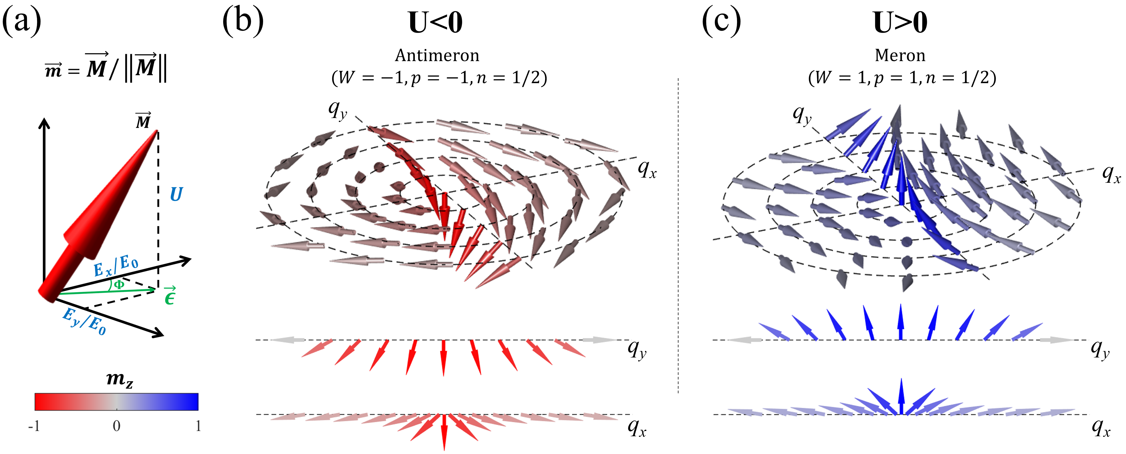
Figure 3: (a) Three-dimensional vector $\bm{M}$ which is composed of the polarization vector $\bm{\epsilon}=(E_{x},E_{y})/E_{0}$, and the band index $U$ as the vertical coordinate. The pseudo-spin $\bm{m}$ is then defined by $\bm{m}=\bm{M}/||{\bm{M}||}$. (b,c) The topological transition from antimeron texture (b) to (c) meron texture of the pseudo-spin $\bm{m}$ through the band inversion. The upper panels of (b,c) show the texture of $\bm{m}$ in the momentum space, while the lower panels show the texture of $\bm{m}$ along the $q_{x}$ and $q_{y}$ axes.

We notice that the energy of the dark mode is very sensitive to the aspect ratio $w/a$ while the one of the bright mode is not. In particular, Figure. 1 (d) shows that the dark mode can be tuned continuously across the bright mode when scanning the aspect ratio, corresponding a tuning of $U$ from $-0.01$ to $0.01$. To demonstrate the band inversion experimentally, we present the following results of two configurations corresponding to $U=\pm 0.005$. Their band structures along the two symmetry directions are experimentally obtained by angle-resolved reflectivity contrast measurements, and numerically calculated by Rigorous coupled-wave analysis (RCWA) simulations[34]. These band structures are represented in Fig. 1(e,g), showing perfect agreement between experimental and simulation data. For the dispersions along $q_{x}$ (with $q_{y}=0$), the dark branch is revealed by its signal vanishing at $\Gamma$ point, while for the dispersion along $q_{y}$ (with $q_{x}\approx 0$), it corresponds to the branch exhibiting sharp linewidth and weaker signal. These results clearly evidenced the band inversion when $U$ switches sign. Finally, the dispersion surface $\hat{\omega}(q_{x},q_{y})$ is tomographically reconstructed by putting together a mega-data of angle-resolved reflectivity contrast measurement along different orientation sets (see Methods and Supplemental Materials for the detailed experimental setup). The experimental data and simulation results of the two-mode surfaces before and after the band inversion, shown in Fig. 1(f,h), exhibit again a perfect agreement.

We now focus on the polarization vortex pinned at the symmetry-protected BIC undergoing band inversion. Such a vortex is characterized by the accumulation of the orientation angle $\phi(\bm{q})$, the orientation of the farfield polarization corresponding to the dark branch, when encircling the symmetry-protected BIC. The pattern $\phi(\bm{q})$ can be analytically calculated from the eigenvectors of the effective Hamiltonian (1) and one may show that the vortex winding number, defined by[16] $W=\frac{1}{2\pi}\oint_{\mathcal{C}}d\bm{q}\nabla_{\bm{q}}\phi$, is simply (see Supplemental Materials for full derivation):

$$W=sgn(U).$$ (2)

The result suggests that the vortex winding number changes sign after the band inversion and thus is not a conservative quantity. It is quite surprising because most of the reported works in the literature suggest the conservation of BIC winding number, which is a topological invariant. To verify experimentally and numerically this intriguing feature, we perform angle-resolved reflectivity contrast measurements and FEM simulations in different polarizations to obtain the tomography reconstruction of the farfield polarization pattern for both photonic branches. The results, presented in Fig. 2, convincingly demonstrate the change of sign of winding number after the band inversion. Indeed, while in the case of the bright mode, no polarization vortices can be observed in the farfield (see Fig. 2 (a) and (d)), the dark mode exhibits a polarization vortex whose winding direction switches when $U$ changes sign, confirming that the winding number is not conserved through the band inversion mechanism and therefore is not a preserved topological number (see Fig. 2 (b) and (c)).

Since the symmetry-protected BIC switches band and the sign of its winding number under band inversion, we propose a definition of a non-Hermitian topological charge that combines the winding number of symmetry-protected BICs and their band index $p=sgn(U)$ defined through the dimensionless diffracting coupling strength. We first consider a three-dimensional vector $\bm{M}$ which is composed of the normalized electric field $\bm{\epsilon}=(E_{x},E_{y})/E_{0}$ and the dimensionless diffracting coupling strength $U$ (see fig. 3 (a)). Here, $E_{x}(q_{x},q_{y})$ and $E_{y}(q_{x},q_{y})$ are electric field amplitudes in the farfield of the photonic lattice, and $E_{0}$ is the amplitude of the confined electric field of TE-guided mode in non-corrugated structure (More information in the theoretical section of the Supplemental Materials). This vector represents both the polarization vortices in its in-plane component, and band-flip in its out-of-plane component. Intuitively, the dynamic of our non-Hermitian band structures is captured by the precession in momentum space of the pseudo-spin that is defined by $\bm{m}=\bm{M}/||{\bm{M}||}$. Indeed, the lower panels in Figs. 3 (b) and (c) present the pseudo-spin $\bm{m}$ along the $q_{x}$ and $q_{y}$ axes before (b) and after (c) the band inversion. At $\Gamma$ point $(q_{x}=q_{y}=0)$, because of the nature of the symmetry-protected BICs, the polarization is not defined and $\bm{\epsilon}=(0,0)$. As a consequence, the pseudo-spin only has a vertical component $m_{z}$ and is oriented in the direction determined by the band index: $\bm{m}=(0,0,p)$. Away from the $\Gamma$ point, for $q=\sqrt{q_{x}^{2}+q_{y}^{2}}\gg U$, the norm of the polarization vector $\bm{\epsilon}$ is non-null and becomes much greater than $U$. Consequently, the pseudo-spin $\bm{m}$ is oriented in the plane, and its vertical component $m_{z}$ is close to zero, resulting in a half flip of the pseudo-spin $\bm{m}$ along the $q_{x}$ and $q_{y}$ axes. The upper panels of Figs. 3 (b) and (c) show the pseudo-spin $\bm{m}$ in momentum space before (b) and after (c) the band inversion. As described previously, the pseudo-spin $\bm{m}$ is half flipped in the vertical direction along the radial axes, while its radial components depend on the polarization vector winding around the BIC at $q_{x}=q_{y}=0$ as shown in Fig. 2. The combination of the half-flip of the vertical component $m_{z}$ and the winding of the polarization vector $\bm{\epsilon}$ results in a precession of the pseudo-spin $\bm{m}$ around the BIC, which can be described as a skyrmion in the momentum space: the precession of a flipping magnetic spin, and we use the definition of the skyrmion number [31]

$$n=\frac{1}{4\pi}\int dq_{x}dq_{y}\bm{m}\cdot\left(\frac{\partial\bm{m}}{\partial q_{x}}\times\frac{\partial\bm{m}}{\partial q_{y}}\right).$$ (3)

The skyrmion number represents the number of times the pseudo-spin winds around the unit sphere; here is $n=pW/2=1/2$ (from the half-flip of the pseudo-spin) corresponding to a meron. We note that the usual definition of pseudo-magnetic moment for photonic skyrmion number is only the polarization vector with the pseudo-spin given by the circular polarization degree [35, 36]. Here the polarization vector of our photonic mode is purely linear (see Fig.2) and only contributes to the in-plane component of $\bm{m}$, and the pseudo-spin is purely related to the band order. Interestingly, as shown in Figs. 3 (b) and (c), the pseudo-spin texture switchs from anti-meron to meron [37] through the band inversion but its skyrmion number of $1/2$ is conserved and can be considered as the definition of non-Hermitian topological charges of symmetry-protected BICs. The skyrmion number defined in this paper reminds us of the definition of skyrmion number in the two-band model of Chern insulator [28], in which the skyrmion number determines the Hall conductance. However, the skyrmion number (and thus the Hall conductance) defined in the model of Ref [28] can change after a band inversion. Therefore, the definition of our skyrmion number is not directly related to the skyrmion number in Chern insulators.

In conclusion, we have shown experimentally that the winding number of the polarization around the symmetry-protected bound state in the continuum (BIC) of leaky photonic modes in a 1D optical lattice is not a conserved quantity as it changes sign during a band inversion. The experimental results were perfectly matched with numerical simulations and are nicely explained with a model of effective Hamiltonian. Our observations showed that the winding number of polarization vortex is not a topological constant in the general case. Consequently, we suggested combining the winding number and the band index to redefine the topological number as a skyrmion number in the momentum space. In our proposal, the band index can be interpreted as the direction of the pseudo-spin at the origin, leading to a meron-like texture in the momentum space. This picture associates the band inversion with a transformation between anti-meron and meron topological spin texture while always conserving the half-charge skyrmion number. Here our skyrmion number plays a similar role as the total Chern number in topological insulators, where the total Chern number is preserved before and after band inversion. In future work, we will apply our formalism to photonic band structures with multiple BICs. We expect the definition of skyrmion number in this paper can be applied to analyze the singularities of other non-Hermitian topological systems [38].

Acknowledgement

The authors thank Shanhui Fan and Pierre Delplace for fruitful discussions.The work is partly funded by the French National Research Agency (ANR) under the project POPEYE (ANR-17-CE24-0020) and the IDEXLYON from Université de Lyon, Scientific Breakthrough project TORE within the Programme Investissements d’Avenir (ANR-19-IDEX-0005). DXN was supported partly by Brown Theoretical Physics Center and by IBS-R024-D1.

Author contributions

H.S.N and L.F initiated the research project and supervised throughout the project. All experimental measurements as well as their analysis, were performed by P.B. The sample was designed and fabricated by L.F. The experimental setup was built by H.S.N and P.B. Effective Hamiltonian model were developed by D.X.N, X.L, P.V and H.S.N. Numerical simulations were performed by P.B and T.B. All authors discussed the results and were involved in writing the manuscript.

Supplementary Information is available for this paper.

Correspondence and requests for materials should be addressed to Paul Bouteyre, Lydie Ferrier and Hai Son Nguyen.

Mehods

Sample fabrication: The bottom Bragg mirror is constituted by 4 $\lambda$/4n pairs of amorphous silicon and silica, deposited by using PECVD (Plasma Enhanced Chemical Vapor Deposition) on a silicon substrate. The thickness and refractive index of each layers have been characterized by ellipsometry measurements. The periodic metallic patterns on top of the Bragg mirror have been defined by using electron beam lithography followed by a 50nm gold evaporation. All patterns are realeased thanks to a lift-off with acetone at the end of the process.

Experimental set-up: All experimental results are obtained from angle-resolved reflectivity contrast measurements using a home-made Fourier setup. Details of the setups, technical points on tomographic bands reconstruction and polarization orientation measurements are provided in the Supplemental Material.

Numerical simulation: Numerical simulations are performed with Rigorous Coupled-Wave Analysis (RCWA) method and Finite Element Method (FEM). The RCWA simulations have been performed with the S⁴ package provided by the Fan Group at the Stanford Electrical Engineering Department.[34] The FEM simulations have been performed with the Comsol software.

— SUPPLEMENTAL MATERIAL —

I Theoretical model

In this section, we provide the detailed derivation of the effective Hamiltonian representing leaky Bloch modes in a general photonic lattice of period $a$ along x-axis and exhibiting a lateral mirror symmetry $x\rightarrow-x$, while being invariant by translation along $y$-axis.

I.1 In-plane guides modes in the vicinity of the $\Gamma$ points

In a perturbative approach, the Bloch modes of the photonic lattice can be described in the basis of propagating in-plan guided modes $\lvert\bm{\beta}\rangle$ of an effective medium with $\bm{\beta}$ being the propagation vector of the guided mode. In the vicinity of $\Gamma$ points, we can decompose a given propagation vector $\bm{\beta}$ as:

$$\bm{\beta_{m}}(\bm{k})=\bm{k}+\frac{2\pi m}{a}\bm{u_{x}}$$ (S1)

where $\bm{k}=k_{x}\bm{u_{x}}+k_{y}\bm{u_{x}}$ with $k_{x},k_{y}\ll 2\pi/a$ and $m\in\mathbb{Z}$ is the index of the 1D Brillouin zone along x-axis. We also used $\bm{u_{x}}$ and $\bm{u_{y}}$ as the unit vectors in $\hat{x}$ and $\hat{y}$ directions correspondingly.

Here, we only focus on the band structure in the vicinity of the lowest $\Gamma$ point (i.e. $\Gamma_{1}$ corresponding to $\lvert m\rvert=1$). As sketched in Fig. S1a, each point $(k_{x},k_{y})$ in the first Brillouin zone corresponds to two guided modes $\lvert\bm{\beta_{\pm 1}}\rangle$ with

$$\bm{\beta_{\pm 1}}(\bm{k})=\bm{k}\pm\frac{2\pi}{a}\bm{u_{x}}.$$ (S2)

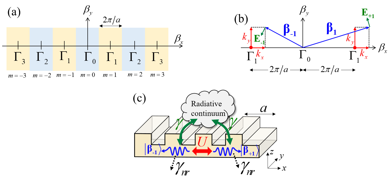
Figure S1: (a) The momentum space in the vicinity of the first $\Gamma$ point of a lattice with period $a$ along x-axis and invariant translation along y-axis is divided into Brilloin zones with index $m\in\mathbb{Z}$.(b) The points $(k_{x},k_{y})$ in the Brillouin zones $m=\pm 1$ correspond to two momentum vector $\bm{\beta_{\pm 1}}=(k_{x}\pm 2\pi m/a)\bm{u_{x}}+k_{y}\bm{u_{y}}$. $E_{\pm 1}$ indicate the corresponding electric field for TE guided modes. (c) Sketch of coupling mechanisms between $\lvert\bm{\beta_{-1}}\rangle$, $\lvert\bm{\beta_{+1}}\rangle$ and the radiative continuum. This includes the diffractive coupling of strength $U$, the radiative losses of rate $\gamma$ and the nonradiative losses of rate $\gamma_{nr}$.

I.1.1 Dispersion characteristic of guided modes

Assuming that the dispersion characteristic in the vicinity of the $\Gamma_{1}$ point is linear with the slope given by the effective group index $n_{g}$, one may show that the dispersion characteristic $\omega_{\pm 1}(k_{x},k_{y})$ is given by:

$$\begin{split}\omega_{\pm 1}(\bm{k})&=\omega_{\Gamma_{1}}+\frac{c}{n_{g}}\left(\lvert\bm{\beta_{\pm 1}}(\bm{k})\rvert-\frac{2\pi}{a}\right)\\ &\approx\omega_{\Gamma_{1}}\pm\frac{c}{n_{g}}k_{x}+\frac{ca}{4\pi n_{g}}k_{y}^{2}\end{split}$$ (S3)

where $c$ is the speed of light and $\omega_{\Gamma_{1}}$ is the pulsation of this guided mode at $\Gamma_{1}$ point.

It is preferable to work with dimensionless quantities. We thus redefine the wavevectors, as well as the pulsations as:

$$\bm{q}=\bm{k}a/2\pi$$ (S4)

and

$$\hat{\omega}_{\pm 1}(\bm{q})=\left(\omega_{\pm 1}(\bm{k})-\omega_{\Gamma_{1}}\right)a/2\pi c.$$ (S5)

Using this quantity instead of $\bm{k}$ and $\omega_{\pm 1}$, the dispersion characteristic (S3) can be rewritten as:

$$\hat{\omega}_{\pm 1}(\bm{q})\approx\pm\frac{q_{x}}{n_{g}}+\frac{q_{y}^{2}}{2n_{g}}$$ (S6)

where $q_{x}=k_{x}a/2\pi$ and $q_{y}=k_{y}a/2\pi$.

I.1.2 Polarization vector of the guided modes

Polarizations of guided modes are classified into TE and TM modes (i.e. the electric field $\bm{E}$ and magnetic field $\bm{H}$ are in-plan and perpendicular to the propagation vector respectively). Here we suppose that there is only one type of guided modes in the spectral range of interest, thus the setup is with single polarization. Moreover, for the sake of simplicity, in this work, we only consider TE modes, knowing that a similar derivation can be obtained for TM modes. For the propagation vector from (S2), the corresponding polarization vector $\bm{u_{\pm 1}}$ is given by $\bm{u}_{\pm 1}\cdot\bm{\beta}_{\pm 1}=0$, leading to:

$$\bm{u_{\pm 1}}(\bm{q})=\cos\theta_{\pm 1}\bm{u_{x}}+\sin\theta_{\pm 1}\bm{u_{y}},$$ (S7)

with

$$\left(\cos\theta_{\pm 1},\sin\theta_{\pm 1}\right)=\frac{\left(-q_{y},q_{x}\pm 1\right)}{\sqrt{(q_{x}\pm 1)^{2}+q_{y}^{2}}}$$ (S8)

I.2 Construction and Analysis of the effective non-Hermitian Hamiltonian

I.2.1 Coupling mechanisms: diffractive coupling and radiative coupling

Now the implementation of a periodic corrugation will induce a coupling $U$ between $\lvert\bm{\beta_{-1}}\rangle$ and $\lvert\bm{\beta_{+1}}\rangle$. Each of them also couples to the radiative continuum with the coupling strength $\gamma$ (see Fig. S1b). In a general case with a presence of non-radiative losses (if the structures include lossy materials such as metals or absorptive dielectrics), the total losses would be increased by an amount $\gamma_{nr}$. As consequence, in the basis $\Psi=\left(\lvert\bm{\beta_{+1}}\rangle,\lvert\bm{\beta_{-1}}\rangle\right)$, the system can be described by the following effective non-Hermitian Hamiltonian:

$$H(\bm{q})=\left(\begin{matrix}\hat{\omega}_{+1}&U\\ U&\hat{\omega}_{-1}\end{matrix}\right)+i\left(\begin{matrix}\gamma+\gamma_{nr}&\gamma\cos\alpha\\ \gamma\cos\alpha&\gamma+\gamma_{nr}\end{matrix}\right)$$ (S9)

The first term of $H$ is Hermitian, describing the free oscillation of each mode and the coupling between them via diffractive coupling. The second term of this Hamiltonian is anti-Hermitian. Its diagonal components describe the total losses including both radiative an non-radiative ones; while its anti-diagonal components describes the coupling between $\lvert\bm{\beta_{+1}}\rangle$ and $\lvert\bm{\beta_{-1}}\rangle$ via the radiative continuum. The coefficient $\cos\alpha=\bm{u_{-1}}.\bm{u_{+1}}$ is due to the fact that only the same electric field component can interfere. We note that in the limit of $q_{x},q_{y}\ll 1$, this coefficient can be effectively replaced by $q_{y}^{2}-1$.

I.2.2 Non-Hermitian Hamiltonian: Eigenvalues of Quasi-normal eigenmodes

Using the Pauli matrices $\sigma_{1}=\begin{pmatrix}0&1\\ 1&0\end{pmatrix}$, $\sigma_{3}=\begin{pmatrix}1&0\\ 0&-1\end{pmatrix}$, the Hamiltonian (S9) can be rewritten as:

$$H=d_{0}\mathbb{I}_{2}+d_{1}\sigma_{1}+d_{3}\sigma_{3}$$ (S10)

where

$$d_{0} =\frac{q_{y}^{2}}{2n_{g}}+i\left(\gamma+\gamma_{nr}\right),$$ (S11)

$$d_{1} =U+i\gamma\cos\alpha,$$ (S12)

$$d_{3} =\frac{q_{x}}{n_{g}}.$$ (S13)

.

The eigenvalues $\Omega_{\pm}$ and corresponding eigenstates $\lvert\pm\rangle$ of (S10) is given by:

$$\Omega_{\pm}=d_{0}\pm\sqrt{d_{1}^{2}+d_{3}^{2}},$$ (S14)

and

$$\lvert\pm\rangle=\left(\begin{matrix}1\\ C_{\pm}\end{matrix}\right)$$ (S15)

with

$$C_{\pm}=-\frac{d_{3}}{d_{1}}\pm\sqrt{\left(\frac{d_{3}}{d_{1}}\right)^{2}+1}.$$ (S16)

As eigenmodes of a non-Hermitian system, $\lvert\pm\rangle$ are quasinormal modes[39] with many mathematical difficulties, for example the way of normalization. Another unusual behaviour of these quasinormal modes is that in general $\lvert+\rangle$ and $\lvert-\rangle$ are not orthogonal between each other. There are two peculiar configurations:

• $d_{3}=\pm id_{1}$ : Simultaneous coalescence of eigenvalues and eigenstates: $\Omega_{+}=\Omega_{-}$ and $\lvert+\rangle=\lvert-\rangle$. This configuration corresponds to Exceptional points[40, 41, 42].

• $d_{3}=0$ : The eigenmodes become normal with $C_{\pm}=\pm 1$. In this configuration, $\lvert+\rangle$ and $\lvert-\rangle$ are two orthogonal states as the ones in Hermitian system.

I.3 Photonic band structures and Farfield polarizations

I.3.1 Complex eigenvalues of Bloch resonances and band inversion mechanism

The explicit form of eigenvalues $\Omega_{\pm}$ are given by:

$$\Omega_{\pm}(\bm{q}) =\frac{q_{y}^{2}}{2n_{g}}+i\left(\gamma+\gamma_{nr}\right)\pm\sqrt{\frac{q_{x}^{2}}{n_{g}^{2}}+\left(U+i\gamma\cos\alpha\right)^{2}}$$

$$=\hat{\omega}_{\pm}+i\gamma_{r\pm}$$ (S17)

The real part $\hat{\omega}_{\pm}$ of $\Omega_{\pm}(\bm{q})$ corresponds to the normalized eigen-frequency. The imaginary counter part $\gamma_{\pm}$ corresponds to the losses including both radiative and nonradiative losses. Finally, the radiative losses $\gamma_{r\pm}$ corresponding to the leaking of these eigenmodes to the radiative continuum) can be extracted by taking out the nonradiative part from the total losses (i.e. subtracting $\gamma_{nr}$ from $\gamma_{\pm}$). One may show that:

$$\hat{\omega}_{\pm}(\bm{q}) \approx\frac{q_{y}^{2}}{2n_{g}}\pm U\left[1+\frac{q_{x}^{2}}{2n_{g}(U^{2}+\gamma^{2})}\right],$$ (S18a)

$$\gamma_{r\pm}(\bm{q}) \approx\gamma\left[1\mp 1\pm\frac{q_{x}^{2}}{2n_{g}(U^{2}+\gamma^{2})}\pm q_{y}^{2}\right]$$ (S18b)

for $q_{x},q_{y}\ll 1$.

Eq. (S18a) describes band dispersion of the eigenmodes in the vicinity of the two band-edges. It shows that the gap separating the two bands amounts to 2$U$. Moreover, the curvature of the dispersion of $\lvert+\rangle$ has the same sign as the one of $U$. As consequence, for each value of $q_{y}$, we can define a band inversion corresponding to a “swapping” between two band dispersion along $q_{x}$ when $U\rightarrow-U$. If $U>0$, the upper branch corresponds to $\lvert+\rangle$ and if $U<0$, the upper branch corresponds to $\lvert-\rangle$.

Now we will show that the band inversion concept is applied not only for the band dispersion but also for whole the complex eigenvalues with complex gap. Indeed, from (I.3.1), for a given $q_{x}$ and for $\forall q_{y}\ll 1$, the two complex eigenvalues are separated by:

$$\kappa(q_{x})\approx 2\sqrt{\frac{q_{x}^{2}}{n_{g}^{2}}+\left(U-i\gamma\right)^{2}}$$ (S19)

The gap $\Delta$ is defined by the minimum of $|\kappa(q_{x})|$. One may show that this gap corresponds to the value $q_{x}=\pm n_{g}\sqrt{max(\gamma^{2}-U^{2},0)}$, and is given by:

$$\begin{cases}|U|>\gamma:\;\;\Delta=2(U-i\gamma)\\ |U|\leq\gamma:\;\;\Delta=2\left[sgn(U)-i\right]\sqrt{|U|\gamma}.\end{cases}$$ (S20)

As consequence, the system is always gapped except when $U=0$. When sweeping $U$ from negative to positive, the complex gap is closed at $U=0$ and then reopened again as soon as $U>0$. We note that $U=0$ corresponds to the Exceptional Points configuration mentioned in the previous section.

Finally, from (S18b), we note that $\gamma_{r+}=0$ at $q_{x}=q_{y}=0$, and increasing as $q_{x}^{2}$ and $q_{y}^{2}$. As consequence $\lvert+\rangle$ is a BIC at $q_{x}=q_{y}=0$. Since this state can still exhibit losses via nonradiative channel, we prefer to call it dark state to underline the nonradiating nature of $\lvert+\rangle$. Logically, the state $\lvert-\rangle$ will be refereed to as bright state since the radiative loss is maximized at $q_{x}=q_{y}=0$. As a consequence, the band inversion mechanism swaps the bright and the dark states.

I.3.2 Eigenmodes of the effective Hamiltonian

The explicit form of eigenstates $\lvert\pm\rangle$ are given by:

$$\lvert\pm\rangle=\lvert\bm{\beta_{+1}}\rangle+C_{\pm}\lvert\bm{\beta_{-1}}\rangle$$ (S21)

with :

$$C_{\pm}=-\frac{q_{x}}{n_{g}(U-i\gamma\cos\alpha)}\pm\sqrt{1+\left[\frac{q_{x}}{n_{g}(U-i\gamma\cos\alpha)}\right]^{2}}.$$ (S22)

At $q_{x}=q_{y}=0$, Eq. (S22) gives us $C_{\pm}\rvert_{q_{x}=q_{y}=0}=\pm 1$, and the eigenmodes is simplifed as:

$$\lvert\pm_{q_{x}=q_{y}=0}\rangle=\lvert\bm{\beta_{+1}}\rangle\pm\lvert\bm{\beta_{-1}}\rangle$$ (S23)

The $\pi$ phase between $\lvert\bm{\beta_{+1}}\rangle_{q_{x}=q_{y}=0}$ and $\lvert\bm{\beta_{-1}}\rangle_{q_{x}=q_{y}=0}$ implies that $\lvert+_{q_{x}=q_{y}=0}\rangle$ is an antisymmetric state while $\lvert-_{q_{x}=q_{y}=0}\rangle$ is a symmetric one. As a consequence, $\lvert+\rangle$ cannot couple to the radiative continuum at $q_{x}=q_{y}=0$ due to symmetry mismatch and is a symmetry protected BIC. This result is quite inline with the one provided by the eigenvalue calculations.

I.3.3 Nearfield pattern

The nearfield of the guided modes $\lvert\bm{\beta_{\pm 1}}\rangle$ is described by plane waves propagating in-plane (x,y) with vertical confinement profile $f(z)$:

$$\begin{split}\bm{\mathcal{E}_{\pm 1}}&=\mathcal{E}_{0}f(z)\exp{\left(i\bm{\beta_{\pm 1}}.\bm{r}_{||}\right)}\bm{u_{\pm 1}}\\ &=\mathcal{E}_{0}f(z)\exp{\left(i\frac{2\pi\bm{q}.\bm{r}_{||}}{a}\right)}\exp{\left(\pm i\frac{2\pi x}{a}\right)}\bm{u_{\pm 1}}\end{split}$$ (S24)

where the propagation wavevector $\bm{\beta_{\pm 1}}$ is from (S2), polarization vector $\bm{u_{\pm 1}}$ is from (S7), $\bm{r}_{||}=(x,y)$ is the in-plane coordinates, $\bm{q}=(q_{x},q_{y})$ is the in-plane wavevector and the constant $\mathcal{E}_{0}$ is a the field amplitude.

Since the eigenmodes $\lvert\pm\rangle$ are given by superpositions of $\lvert\bm{\beta_{+1}}\rangle$ and $\lvert\bm{\beta_{-1}}\rangle$, the nearfield patterns of $\lvert\pm\rangle$ are also dictated by the same superposition rule:

$$\begin{split}\bm{\mathcal{E}_{\pm}}&=\bm{\mathcal{E}_{+1}}+C_{\pm}\bm{\mathcal{E}_{-1}}\\ &=\mathcal{E}_{0}f(z)\exp{\left(i\frac{2\pi\bm{q}.\bm{r}_{||}}{a}\right)}\left[\exp{\left(i\frac{2\pi x}{a}\right)}\bm{u_{+1}}+C_{\pm}\exp{\left(-i\frac{2\pi x}{a}\right)}\bm{u_{-1}}\right].\end{split}$$ (S25)

At $\bm{q}=\bm{0}$, Eqs. (S7),(S8) and(S22) imply that $\bm{u_{\pm 1}}(\bm{q}=\bm{0})=\pm\bm{u_{y}}$ and $C_{\pm}(\bm{q}=\bm{0})=\pm 1$. As a consequence, the nearfield is given by::

$$\begin{cases}\bm{\mathcal{E}_{+}}(\bm{q}=\bm{0})&=2i\mathcal{E}_{0}f(z)\sin{\left(\frac{2\pi x}{a}\right)}\bm{u_{y}}\;\;\rightarrow\textit{ odd parity with respect to the lateral mirror symmetry}\\ \bm{\mathcal{E}_{-}}(\bm{q}=\bm{0})&=2\mathcal{E}_{0}f(z)\cos{\left(\frac{2\pi x}{a}\right)}\bm{u_{y}}\;\;\rightarrow\textit{ even parity with respect to the lateral mirror symmetry}\end{cases}$$ (S26)

As a consequence, $\lvert+\rangle(\bm{q}=\bm{0})$ cannot couple to the radiative continuum due to symmetry mismatch with plane waves of even parity in this continuum. Otherwise, the coupling between $\lvert-\rangle(\bm{q}=\bm{0})$ and the radiative continuum is permitted. Therefore $\lvert+\rangle(\bm{q}=\bm{0})$ corresponds to symmetry-protected BIC. We note that the nearfield distribution given by (S26) is in perfect aggrement with the numerical simulation results in Fig.  1(c) of the main text.

I.3.4 Polarization pattern of the farfield in momentum space

The Bragg scattering mechanism due to periodic corrugation fold the guided modes $\lvert\bm{\beta_{1}}\rangle$ from $\bm{\beta_{\pm 1}}=\bm{k}\pm\frac{2\pi}{a}\bm{u_{x}}$ to the same wavevector $\bm{k}$. As a consequence, these guided modes once folded radiate to the freespace as plane wave with $\bm{k}$ as the in-plane component. In the vicinity of the normal emission, these radiating waves are approximately described as plane waves of the same wavevector $\frac{\omega_{\Gamma_{1}}}{c}\bm{u_{z}}$ while preserving the polarization $\bm{u_{\pm 1}}$ of the unfolded modes:

$$\bm{E_{\pm 1}}(\bm{q})=E_{0}\exp\left(i\omega_{\Gamma_{1}}z/c\right)\bm{u_{\pm 1}}(\bm{q})$$ (S27)

where the amplitude $E_{0}$ of radiative waves is proportional to the amplitude $mathcal{E_{0}}$ of the unfolded modes.

The farfield patterns of the hybrid modes $\lvert\pm\rangle$ are also dictated by the same superposition rule of the egeinmodes and nearfield pattern:

$$\begin{split}\bm{E_{\pm}}(\bm{q})&=\bm{E_{+1}}(\bm{q})+C_{\pm}\bm{E_{-1}}(\bm{q})\\ &=E_{0}\exp\left(i\omega_{\Gamma_{1}}z/c\right)\left(\bm{u_{+1}}+C_{\pm}\bm{u_{-1}}\right).\end{split}$$ (S28)

We remind that at $\bm{q}=\bm{0}$, $\bm{u_{\pm 1}}(\bm{q}=\bm{0})=\pm\bm{u_{y}}$ and $C_{\pm}(\bm{q}=\bm{0})=\pm 1$. Therefore, the farfield at $\Gamma$ point is given by:

$$\begin{cases}\bm{E_{+}}(\bm{q}=\bm{0})&=0\;\;\rightarrow\textit{ destructive interference}\\ \bm{E_{-}}(\bm{q}=\bm{0})&=2E_{0}\exp\left(i\omega_{\Gamma_{1}}z/c\right)\bm{u_{y}}\,\rightarrow\textit{ constructive interference}\end{cases}$$

This result shows that the farfield of $\lvert+\rangle$ has a singularity at $q_{x}=q_{y}=0$, which is in good agreement with its dark nature demonstrated previously.

For an arbitrary coordinate $(q_{x},q_{y})$, the electric field $\bm{E_{\pm}}$ is reconstructed in Cartesian basis as:

$$\bm{E_{\pm}}=E_{x,\pm}\bm{u_{x}}+E_{y,\pm}\bm{u_{y}}$$ (S29)

where the complex components $E_{x,\pm}$ and $E_{y,\pm}$ are given by:

$$E_{x,\pm} =E_{0}\exp\left(i\omega_{\Gamma_{1}}z/c\right)\left(\cos\theta_{+1}+C_{\pm}\cos\theta_{-1}\right),$$ (S30a)

$$E_{y,\pm} =E_{0}\exp\left(i\omega_{\Gamma_{1}}z/c\right)\left(\sin\theta_{+1}+C_{\pm}\sin\theta_{-1}\right).$$ (S30b)

where $\sin\theta_{\pm 1}$, $\cos\theta_{\pm 1}$ and $C_{\pm}$ are from Eqs. (S8) and(S22). The orientation (i.e. angle $\phi_{\pm}$) of $\bm{E_{\pm}}(\bm{q})$ with respect to $\bm{u_{x}}$ (see Fig.S2a) is given by:[43]

$$\tan 2\phi_{\pm}=\frac{2\text{Re}(E_{x,\pm}^{*}.E_{y,\pm})}{|E_{x,\pm}|^{2}-|E_{y,\pm}|^{2}}$$ (S31)

The ellipticity of the polarization, described by angle $\chi_{\pm}$ (see Fig.S2a), is given by: [43]

$$\sin 2\chi_{\pm}=\frac{2\text{Im}(E_{x,\pm}^{*}.E_{y,\pm})}{|E_{x,\pm}|^{2}+|E_{y,\pm}|^{2}}$$ (S32)

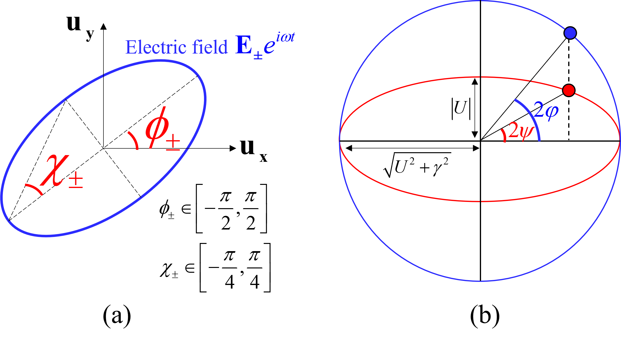
Figure S2: (a) Elliptic polarization of light with orientation angle $\phi$ and ellipticity $\chi$. (b) Graphical presentation of the 1:1 correspondence between $\varphi$ and $\psi$.

I.3.5 Winding number of the polarization vortex

From the orientation angle $\phi_{\pm}(\bm{q})$, the winding number around $q_{x}=q_{y}=0$ of the vector field $\bm{E_{\pm}}(\bm{q})$ is defined as:

$$W_{\pm}=\frac{1}{2\pi}\oint_{\mathcal{C}}d\bm{q}\nabla_{\bm{q}}\phi_{\pm}.$$ (S33)

where $\mathcal{C}$ is a closed circulation encircling $q_{x}=q_{y}=0$. One may uses directly Eq. (S31) and calculating $W_{\pm}$ for a arbitrary path $\mathcal{C}$. However, knowing that the only possible singularity is located at $q_{x}=q_{y}=0$, $W_{\pm}$ does not depend on the choice of $\mathcal{C}$, we will choose an adequate $\mathcal{C}$ so that the integral can be easily calculated. To do so, we define the complex number $z=\rho e^{i\varphi}$ with:

$$\text{Re}(z) =\rho\cos\varphi=\frac{q_{x}}{2n_{g}\sqrt{U^{2}+\gamma^{2}}},$$ (S34a)

$$\text{Im}(z) =\rho\sin\varphi=q_{y}.$$ (S34b)

The winding number will be calculated by encircling in the counter-clockwise direction around $q_{x}=q_{y}=0$ when fixing $\rho\ll 1$ constant and varying $\varphi$. The condition $\rho\ll 1$ implies that $\lvert q_{x}\rvert,\lvert q_{y}\rvert\ll 1$. Thus from (S8),(S22), we can approximate:

$$\begin{cases}\sin\theta_{\pm 1}\approx\pm 1\\ \cos\theta_{\pm 1}\approx-\rho\sin\varphi\\ C_{\pm}\approx\pm 1-2\rho\cos\varphi\frac{U+i\gamma}{\sqrt{U^{2}+\gamma^{2}}}\end{cases}$$ (S35)

Injecting to (S30a),(S30b), that leads to:

– For the $\lvert-\rangle$ state :

$$\frac{E_{x,-}}{E_{0}} \approx 2\rho^{2}\cos\varphi\sin\varphi\frac{U+i\gamma}{\sqrt{U^{2}+\gamma^{2}}}\approx 0$$

$$\frac{E_{y,-}}{E_{0}} \approx 2+2\rho\cos\varphi\frac{U+i\gamma}{\sqrt{U^{2}+\gamma^{2}}}\approx 2$$

$$\rightarrow\text{always vertical polarization,i.e. }\phi_{-}=\pi/2$$

$$\rightarrow\boxed{W_{-}=0}.$$

– For the $\lvert+\rangle$ state :

$$\frac{E_{x,+}}{E_{0}} \approx-2\rho\sin\varphi$$

$$\frac{E_{y,+}}{E_{0}} \approx 2\rho\cos\varphi\frac{U+i\gamma}{\sqrt{U^{2}+\gamma^{2}}}$$

using (S31), we obtain then:

$$\tan 2\phi_{+} =\tan 2\varphi\frac{U}{\sqrt{U^{2}+\gamma^{2}}}$$

$$=sgn(U)\tan{2\psi}$$

where angle $\psi$ is obtained from $\varphi$ by shrinking an ellipse of semi-major axe $\sqrt{U^{2}+\gamma^{2}}$ and semi-mino axe $|U|$ into a circle of radius $\sqrt{U^{2}+\gamma^{2}}$ (see Fig.S2b). Hence

$$\phi_{+}=sgn(U)\psi$$ (S36)

Moreover, we note that the pathway $\mathcal{C}$ of counter-clockwise direction around $q_{x}=q_{y}=0$ corresponds to $\varphi$ varies from 0 to 2$\pi$, due to the definition (S34a) and (S34b). Moreover, as indicated in Fig.S2b, $\psi$ will also sweep from 0 to 2$\pi$. Thus

$$\begin{split}\oint_{\mathcal{C}}d\varphi=2\pi.sgn(U)\rightarrow\boxed{W_{+}=sgn(U)}.\end{split}$$ (S37)

As a matter of fact, the winding number of the polarization vortex associated with $\lvert+\rangle$ is given by the sign of $U$, thus changes sign after a band-inversion (i.e. $U$ changes sign).

II Experimental methods

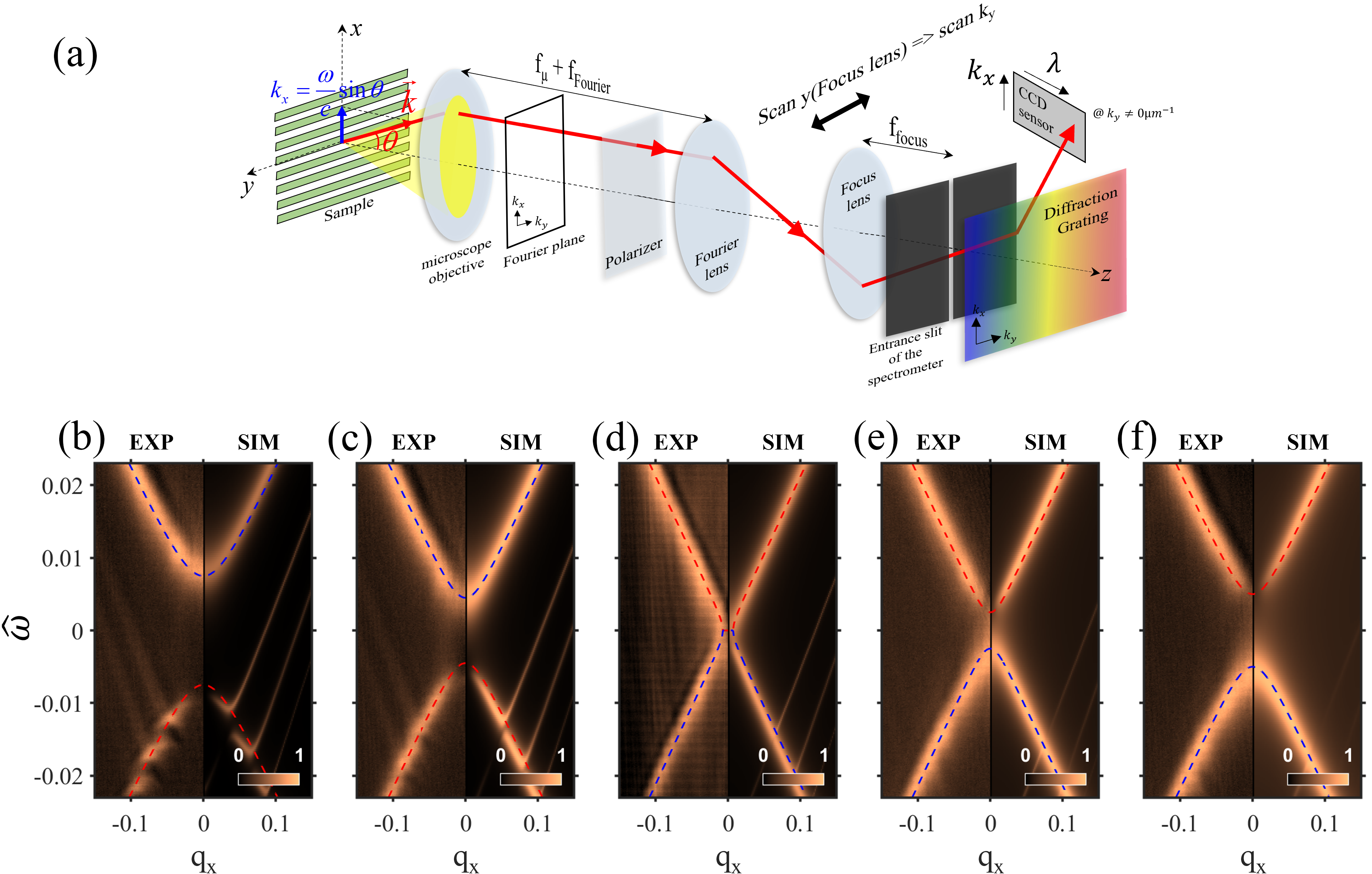
Figure S3: Experimental setup (a) Sketch of the home-made Fourier set-up for the angle-resolved reflectivity measurements. Band inversion mechanism (b to f) $k_{x}$-resolved contrast reflectivity maps of five different structures with different aspect ratios $w/a$ (diffractive coupling $U$): (b) 0.34 (-0.0075) (c) 0.4 (-0.0045) (d) 0.425 (0) (e) 0.47 (0.0025) (f) 0.505 (0.005). For the aspect ratios $w/a<0.44$ ($U<0$), the lower branch corresponds to the dark mode (BIC), and the upper branch to the bright mode. When the aspect ratio increases continuously, the dark and bright modes get closer to each other until they form two exceptional points for $w/a=0.44$ ($U=0$). The two modes are swapped when the aspect ratios becomes $w/a>0.44$ ($U>0$), and the two modes move away from each other when the aspect ratio further increases. This process is the band inversion mechanism. (b) and (f) corresponds to the structures studied in the article.

II.0.1 Angle-resolved reflectivity measurements

All experimental results in this work are obtained from angle-resolved reflectivity measurements using a home-made Fourier setup [see Fig.S3 (a)]. The Fourier plane of the structure located at the focal length of the microscope objective is projected with the ’Fourier’ and ’Focus’ lenses to the entrance of the spectrometer. The slit of the spectrometer only selects the Fourier image in the $k_{x}$ direction for a given $k_{y}$, which can be controlled by the y position of the ’focus’ lens. The signal is then dispersed by the spectrometer diffraction grating and collected by a CCD camera resulting in a $k_{x}$-resolved measurement of the bands.

As illustration, Figs. S3 (b) to (f) depicts angle-resolved measurements from five different structures. These structures have been chosen to depict the band inversion mechanism.

II.0.2 Tomographic bands reconstruction

To perform tomographic bands reconstruction, 50 $k_{x}$-resolved measurements for $k_{y}$ varying from $-k_{max}$ to $k_{max}$ were performed for all the structures. For each $k_{x}$-resolved measurements at given $k_{y}$, the measurement is fitted with two Lorentzian functions giving the modes’ wavelength [see blue and red dashed line in Fig. S4 (a)] and amplitude resonances (i.e. intensities). From the modes’ wavelength, we can construct the dispersion surface of the modes as illustrated in Fig. S4 (b).

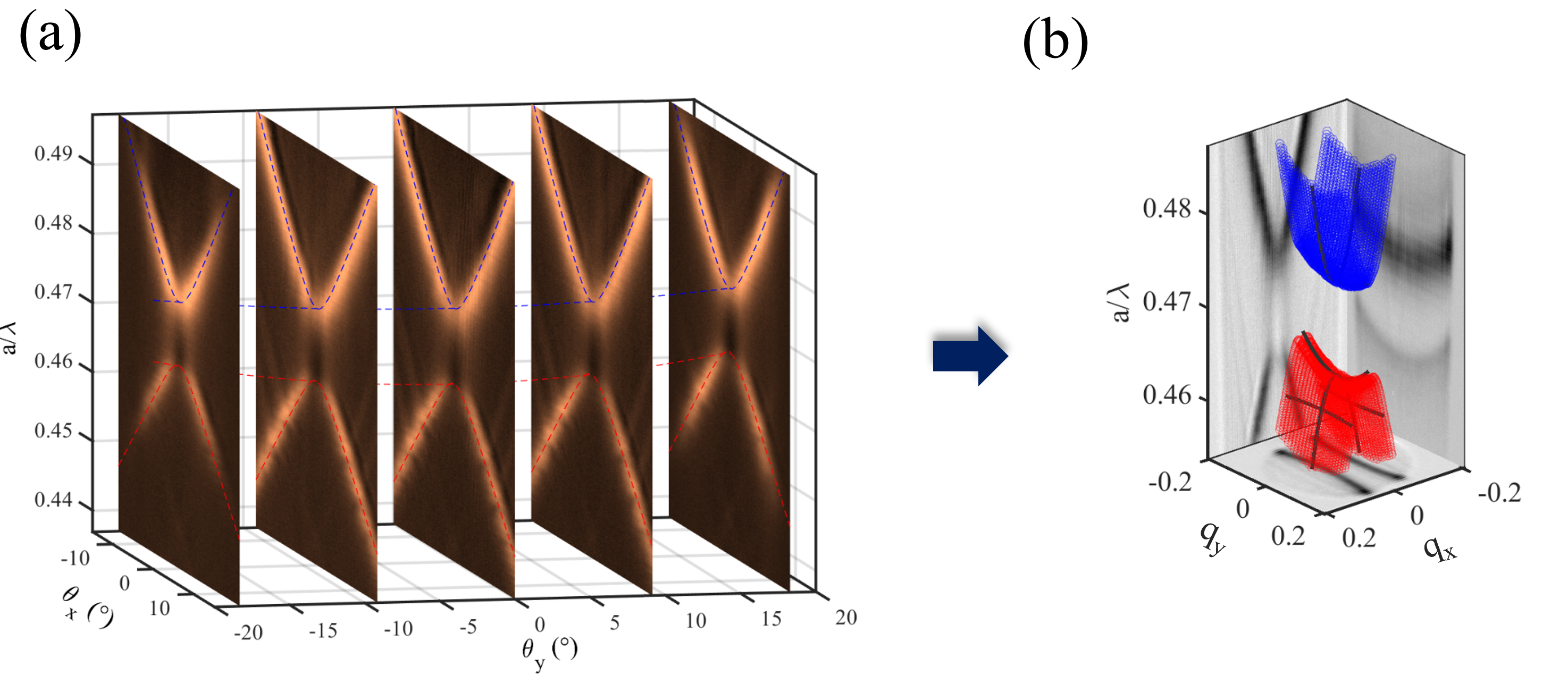
Figure S4: Tomography band reconstruction (a) Sketch illustrating the $k_{x}$-resolved measurements of the optical bands for different $k_{y}$ in the case of the structure with the diffractive coupling strength $U<0$. Only five measurements are shown here for simplicity. For each $k_{x}$-resolved measurements at given $k_{y}$, each $k_{x}$ slices are fitted with two Lorentzian functions giving the modes wavelength $\lambda_{m}(k_{x},k_{y})$ (see blue and red dashed line), as well as their resonant amplitude $I_{m}(k_{x},k_{y})$. (b) Tomographic bands reconstruction of the structure with the diffractive coupling strength $U<0$. The projections in the momentum plane and in the ($k_{x},a/\lambda$) plane are taken from the $k_{y}$-scan measurements presented in this figure. The projection in the ($k_{y},a/\lambda$) plane is taken from additional measurements in which the sample was rotated by 90^∘ to directly measure the $k_{y}$-resolved dispersion at $k_{x}$=0.

II.0.3 Measurement of the polarization vortex

Different polarization elements (polarizers, half-wave plates, quater-wave plates) may be introduced for polarization-resolved measurements. The tomographic experiment is performed for different polarizations to retrieve polarization-resolved intensities of each mode [see Fig. S5 (a,b)]. From these results, we obtain the mapping of Stoke parameters in momentum space [see Fig. S5 (c)]. Finally, from the Stoke parameters, the mapping of the polarization orientation $\Phi$ is retrieved [see Fig. S5 (d)].

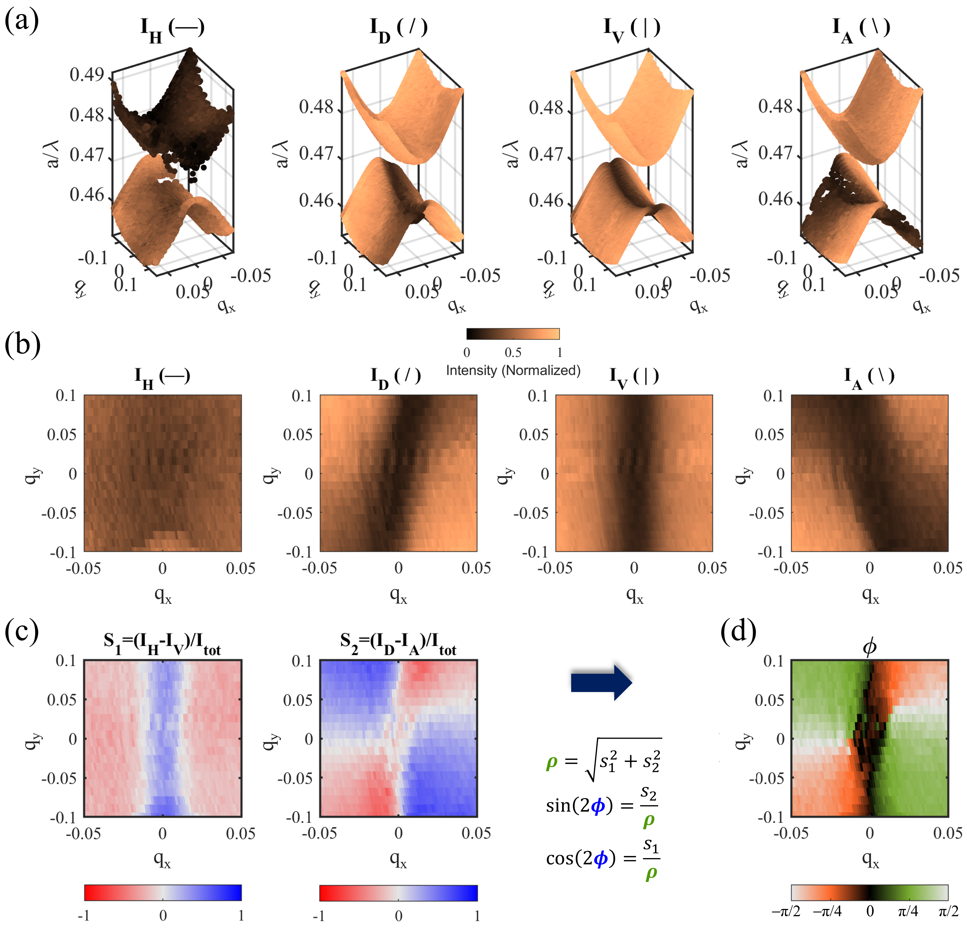
Figure S5: Polarization orientation measurements (a) Tomographic bands reconstruction of the structure with the diffractive coupling strength $U<0$ for four different linear polarizations: Horizontal, Diagonal, Vertical, and Anti-Diagonal. The color-map texture indicates the intensity of the modes at each position in momentum space. A drop in intensity can be observed on the low-energy mode around the BIC at $q_{x}=q_{y}=0$ (b) Momentum-resolved intensity map of the low-energy mode in (a). (c) Momentum-resolved Stokes parameters $S_{1}=(I_{H}-I_{V})/(I_{H}+I_{V})$ and $S_{2}=(I_{D}-I_{A})/(I_{D}+I_{A})$ of the low-energy mode extracted from the intensity map in (b). (d) Farfield polarization orientation of the low-energy mode with a diffractive coupling $U<0$ calculated using the stokes parameters in (c). This method was used to measure the polarization orientation of all the modes studied in the article.

References

- Von Neumann and Wigner [1929] J. Von Neumann and E. Wigner, Über merkwürdige diskrete Eigenwerte, Z. Phys 30, 465 (1929).
- Friedrich and Wintgen [1985a] H. Friedrich and D. Wintgen, Interfering resonances and bound states in the continuum, Physical Review A 32, 3231 (1985a).
- Friedrich and Wintgen [1985b] H. Friedrich and D. Wintgen, Physical realization of bound states in the continuum, Physical Review A 31, 3964 (1985b).
- Cederbaum et al. [2003] L. S. Cederbaum, R. S. Friedman, V. M. Ryaboy, and N. Moiseyev, Conical Intersections and Bound Molecular States Embedded in the Continuum, Physical Review Letters 90, 013001 (2003).
- Thomas et al. [2018] R. Thomas, M. Chilcott, E. Tiesinga, A. B. Deb, and N. Kjærgaard, Observation of bound state self-interaction in a nano-eV atom collider, Nature Communications 9, 4895 (2018).
- Cobelli et al. [2011] P. J. Cobelli, V. Pagneux, A. Maurel, and P. Petitjeans, Experimental study on water-wave trapped modes, Journal of Fluid Mechanics 666, 445 (2011).
- Capasso et al. [1992] F. Capasso, C. Sirtori, J. Faist, D. L. Sivco, S.-N. G. Chu, and A. Y. Cho, Observation of an electronic bound state above a potential well, Nature 358, 565 (1992).
- Nöckel [1992] J. U. Nöckel, Resonances in quantum-dot transport, Physical Review B 46, 15348 (1992).
- Ladrón de Guevara and Orellana [2006] M. L. Ladrón de Guevara and P. A. Orellana, Electronic transport through a parallel-coupled triple quantum dot molecule: Fano resonances and bound states in the continuum, Physical Review B 73, 205303 (2006).
- Hsu et al. [2013] C. W. Hsu, B. Zhen, J. Lee, S.-l. Chua, S. G. Johnson, J. D. Joannopoulos, and M. Soljačić, Observation of trapped light within the radiation continuum, Nature 499, 188 (2013).
- Kodigala et al. [2017] A. Kodigala, T. Lepetit, Q. Gu, B. Bahari, Y. Fainman, and B. Kanté, Lasing action from photonic bound states in continuum, Nature 541, 196 (2017).
- Ha et al. [2018] S. T. Ha, Y. H. Fu, N. K. Emani, Z. Pan, R. M. Bakker, R. Paniagua-Domínguez, and A. I. Kuznetsov, Directional lasing in resonant semiconductor nanoantenna arrays, Nature Nanotechnology 13, 1042 (2018).
- Huang et al. [2020] C. Huang, C. Zhang, S. Xiao, Y. Wang, Y. Fan, Y. Liu, N. Zhang, G. Qu, H. Ji, J. Han, L. Ge, Y. Kivshar, and Q. Song, Ultrafast control of vortex microlasers, Science 367, 1018 (2020).
- Romano et al. [2020] S. Romano, M. Mangini, E. Penzo, S. Cabrini, A. C. De Luca, I. Rendina, V. Mocella, and G. Zito, Ultrasensitive Surface Refractive Index Imaging Based on Quasi-Bound States in the Continuum, ACS Nano 14, 15417 (2020).
- Tittl et al. [2018] A. Tittl, A. Leitis, M. Liu, F. Yesilkoy, D.-Y. Choi, D. N. Neshev, Y. S. Kivshar, and H. Altug, Imaging-based molecular barcoding with pixelated dielectric metasurfaces, Science 360, 1105 (2018).
- Zhen et al. [2014] B. Zhen, C. W. Hsu, L. Lu, a. D. Stone, and M. Soljačić, Topological Nature of Optical Bound States in the Continuum, Physical Review Letters 113, 1 (2014).
- Zhang et al. [2018] Y. Zhang, A. Chen, W. Liu, C. W. Hsu, B. Wang, F. Guan, X. Liu, L. Shi, L. Lu, and J. Zi, Observation of polarization vortices in momentum space, Phys. Rev. Lett. 120, 186103 (2018).
- Doeleman et al. [2018] H. M. Doeleman, F. Monticone, W. den Hollander, A. Alù, and A. F. Koenderink, Experimental observation of a polarization vortex at an optical bound state in the continuum, Nature Photonics 12, 397 (2018).
- Yin and Peng [2020] X. Yin and C. Peng, Manipulating light radiation from a topological perspective, Photon. Res. 8, B25 (2020).
- Jin et al. [2019] J. Jin, X. Yin, L. Ni, M. Soljačić, B. Zhen, and C. Peng, Topologically enabled ultrahigh-Q guided resonances robust to out-of-plane scattering, Nature 574, 501 (2019).
- Liu et al. [2019] W. Liu, B. Wang, Y. Zhang, J. Wang, M. Zhao, F. Guan, X. Liu, L. Shi, and J. Zi, Circularly polarized states spawning from bound states in the continuum, Phys. Rev. Lett. 123, 116104 (2019).
- Yoda and Notomi [2020] T. Yoda and M. Notomi, Generation and annihilation of topologically protected bound states in the continuum and circularly polarized states by symmetry breaking, Phys. Rev. Lett. 125, 053902 (2020).
- Kang et al. [2021] M. Kang, S. Zhang, M. Xiao, and H. Xu, Merging bound states in the continuum at off-high symmetry points, Phys. Rev. Lett. 126, 117402 (2021).
- Kang et al. [2022] M. Kang, L. Mao, S. Zhang, M. Xiao, H. Xu, and C. T. Chan, Merging bound states in the continuum by harnessing higher-order topological charges, Light: Science & Applications 11, 228 (2022).
- Schnyder et al. [2008] A. P. Schnyder, S. Ryu, A. Furusaki, and A. W. W. Ludwig, Classification of topological insulators and superconductors in three spatial dimensions, Phys. Rev. B 78, 195125 (2008).
- Hasan and Kane [2010] M. Z. Hasan and C. L. Kane, Colloquium: Topological insulators, Rev. Mod. Phys. 82, 3045 (2010).
- Ozawa et al. [2019] T. Ozawa, H. M. Price, A. Amo, N. Goldman, M. Hafezi, L. Lu, M. C. Rechtsman, D. Schuster, J. Simon, O. Zilberberg, and I. Carusotto, Topological photonics, Rev. Mod. Phys. 91, 015006 (2019).
- Bernevig et al. [2006] B. A. Bernevig, T. L. Hughes, and S.-C. Zhang, Quantum spin hall effect and topological phase transition in hgte quantum wells, Science 314, 1757 (2006).
- Zhu et al. [2012] Z. Zhu, Y. Cheng, and U. Schwingenschlögl, Band inversion mechanism in topological insulators: A guideline for materials design, Phys. Rev. B 85, 235401 (2012).
- Skyrme [1962] T. Skyrme, A unified field theory of mesons and baryons, Nuclear Physics 31, 556 (1962).
- Heinze et al. [2011] S. Heinze, K. von Bergmann, M. Menzel, J. Brede, A. Kubetzka, R. Wiesendanger, G. Bihlmayer, and S. Blügel, Spontaneous atomic-scale magnetic skyrmion lattice in two dimensions, Nature Physics 7, 713 (2011).
- Ferrier et al. [2019] L. Ferrier, H. S. Nguyen, C. Jamois, L. Berguiga, C. Symonds, J. Bellessa, and T. Benyattou, Tamm plasmon photonic crystals: From bandgap engineering to defect cavity, APL Photonics 4, 106101 (2019).
- Lee and Magnusson [2019] S.-G. Lee and R. Magnusson, Band flips and bound-state transitions in leaky-mode photonic lattices, Phys. Rev. B 99, 045304 (2019).
- Liu and Fan [2012] V. Liu and S. Fan, S4 : A free electromagnetic solver for layered periodic structures, Computer Physics Communications 183, 2233 (2012).
- Guo et al. [2020] C. Guo, M. Xiao, Y. Guo, L. Yuan, and S. Fan, Meron spin textures in momentum space, Phys. Rev. Lett. 124, 106103 (2020).
- Król et al. [2021] M. Król, H. Sigurdsson, K. Rechcińska, P. Oliwa, K. Tyszka, W. Bardyszewski, A. Opala, M. Matuszewski, P. Morawiak, R. Mazur, W. Piecek, P. Kula, P. G. Lagoudakis, B. Piętka, and J. Szczytko, Observation of second-order meron polarization textures in optical microcavities, Optica 8, 255 (2021).
- Yu et al. [2018] X. Z. Yu, W. Koshibae, Y. Tokunaga, K. Shibata, Y. Taguchi, N. Nagaosa, and Y. Tokura, Transformation between meron and skyrmion topological spin textures in a chiral magnet, Nature 564, 95 (2018).
- Zhu et al. [2021] Z. Zhu, C. Li, and J. B. Marston, Topology of rotating stratified fluids with and without background shear flow, arXiv e-prints , arXiv:2112.04691 (2021), arXiv:2112.04691 .
- Lalanne et al. [2018] P. Lalanne, W. Yan, K. Vynck, C. Sauvan, and J.-P. Hugonin, Light interaction with photonic and plasmonic resonances, Laser & Photonics Reviews 12, 1700113 (2018).
- Kawabata et al. [2019a] K. Kawabata, T. Bessho, and M. Sato, Classification of exceptional points and non-hermitian topological semimetals, Phys. Rev. Lett. 123, 066405 (2019a).
- Kawabata et al. [2019b] K. Kawabata, K. Shiozaki, M. Ueda, and M. Sato, Symmetry and topology in non-hermitian physics, Phys. Rev. X 9, 041015 (2019b).
- Bergholtz et al. [2021] E. J. Bergholtz, J. C. Budich, and F. K. Kunst, Exceptional topology of non-hermitian systems, Rev. Mod. Phys. 93, 015005 (2021).
- Dennis [2002] M. Dennis, Polarization singularities in paraxial vector fields: morphology and statistics, Optics Communications 213, 201 (2002).