Local gravitational instability of stratified rotating fluids: 3D criteria for gaseous discs

Abstract

Fragmentation of rotating gaseous systems via gravitational instability is believed to be a crucial mechanism in several astrophysical processes, such as formation of planets in protostellar discs, of molecular clouds in galactic discs, and of stars in molecular clouds. Gravitational instability is fairly well understood for infinitesimally thin discs. However, the thin-disc approximation is not justified in many cases, and it is of general interest to study the gravitational instability of rotating fluids with different degrees of rotation support and stratification. We derive dispersion relations for axisymmetric perturbations, which can be used to study the local gravitational stability at any point of a rotating axisymmetric gaseous system with either barotropic or baroclinic distribution. 3D stability criteria are obtained, which generalize previous results and can be used to determine whether and where a rotating system of given 3D structure is prone to clump formation. For a vertically stratified gaseous disc of thickness $h_{z}$ (defined as containing $\approx$70% of the mass per unit surface), a sufficient condition for local gravitational instability is $Q_{\rm 3D}\equiv\left(\sqrt{\kappa^{2}+\nu^{2}}+c_{\rm s}h_{z}^{-1}\right)/{\sqrt{4\pi G\rho}}<1$, where $\rho$ is the gas volume density, $\kappa$ the epicycle frequency, $c_{\rm s}$ the sound speed, and $\nu^{2}\equiv\rho^{\prime}_{z}p^{\prime}_{z}/\rho^{2}$, where $\rho^{\prime}_{z}$ and $p^{\prime}_{z}$ are the vertical gradients of, respectively, gas density and pressure. The combined stabilizing effects of rotation ($\kappa^{2}$) and stratification ($\nu^{2}$) are apparent. In unstable discs, the conditions for instability are typically met close to the midplane, where the perturbations that are expected to grow have characteristic radial extent of a few $h_{z}$.

1 Introduction

Rotating gaseous structures confined by gravitational potentials are widespread among astrophysical systems on a broad range of scales. Prototypical examples include gaseous galactic discs, accretion discs, and protostellar and protoplanetary discs, but rotation can be non-negligible also in pressure-supported systems such as stars, molecular clouds, galactic coronae and hot atmospheres of galaxy clusters. The confining gravitational potential can be due either only to the gas itself or to a combination of the gas self-gravity and of an external potential. Whenever the gas self-gravity is locally non-negligible with respect to the external potential, the evolution of the rotating fluid depends crucially on whether it is gravitationally stable or unstable. For instance, in galactic discs local gravitational instability is expected to lead to fragmentation, growth of dense gas clumps and eventually to star formation (see e.g. section 8.3 of Cimatti et al., 2019). In protostellar discs, gravitational instability can contribute either directly (via gas collapse) or indirectly (via concentration of dust particles) to the process of planet formation (Kratter & Lodato, 2016). It is thus not surprising that the study of gravitational instability of rotating fluids has a fairly long history in the astrophysical literature.

Gravitational instability in infinitesimally thin discs has been widely studied with fundamental contributions dating back to more than fifty years ago (e.g. Lin & Shu, 1964; Toomre, 1964; Hunter, 1972, and references therein). However, the thin-disc approximation is not justified in many cases. In protostellar discs, the vertical extent of the gas can be substantial (e.g. Law et al., 2022). Also gaseous discs in present-day galaxies can have non-negligible thickness (Yim et al., 2014), and there are indications that disc thickness increases with redshift (Förster Schreiber et al., 2006), though dynamically cold disc are found also in high-redshift galaxies (Rizzo et al., 2021). Thick gaseous discs are observed in present-day dwarf galaxies (e.g. Roychowdhury et al., 2010) and expected in dwarf protogalaxies (Nipoti & Binney, 2015). Moreover, the observational galactic volumetric star formation laws (Bacchini et al., 2019) strongly suggest that the 3D structure of discs has an important role in the process of conversion of gas into stars.

Several authors have tackled the problem of the gravitational instability of non-razor-thin discs, essentially obtaining modifications of the thin-disc stability criteria that account for finite thickness (Toomre, 1964; Romeo, 1992; Bertin & Amorisco, 2010; Wang et al., 2010; Elmegreen, 2011; Griv & Gedalin, 2012; Romeo & Falstad, 2013; Behrendt et al., 2015). 3D systems were studied only under rather specific assumptions: Chandrasekhar (1961) analyzed infinite homogeneous rotating systems, while Safronov (1960), Genkin & Safronov (1975) and Bertin & Casertano (1982) considered homogeneous rotating slabs of finite thickness. Goldreich & Lynden-Bell (1965a, b) accounted in detail for the vertical stratification of the gas distribution, assuming polytropic equation of state (and thus polytropic distributions) with specific values of the polytropic index (see also Meidt 2022).

In this work we address the general problem of the local gravitational stability of rotating stratified fluids. Considering axisymmetric perturbations, we derive 3D dispersion relations and stability criteria for baroclinic and barotropic configurations, as well as for somewhat idealized models of vertically stratified discs.

2 Preliminaries

We perform a linear stability analysis of rotating astrophysical gaseous systems taking into account the self-gravity of the perturbations. Here we introduce the equations on which such analysis is based, and we define the general properties of the unperturbed fluid and of the disturbances.

2.1 Fundamental equations

For our purposes the relevant set of equations consists in the adiabatic inviscid fluid equations combined with the Poisson equation. As it is natural when dealing with rotating system, we work in cylindrical coordinates $(R,\phi,z)$. For simplicity we consider only axisymmetric unperturbed configurations and perturbations, so all derivatives with respect to $\phi$ are null. Under these assumptions the fundamental system of equations reads

$$\begin{split}&\frac{\partial\rho}{\partial t}+\frac{1}{R}\frac{\partial(R\rho u_{R})}{\partial R}+\frac{\partial(\rho u_{z})}{\partial z}=0,\\ &\frac{\partial u_{R}}{\partial t}+u_{R}\frac{\partial u_{R}}{\partial R}+u_{z}\frac{\partial u_{R}}{\partial z}-\frac{u_{\phi}^{2}}{R}=-\frac{1}{\rho}\frac{\partial p}{\partial R}-\frac{\partial\Phi}{\partial R}-\frac{\partial\Phi_{\rm ext}}{\partial R},\\ &\frac{\partial u_{\phi}}{\partial t}+u_{R}\frac{\partial u_{\phi}}{\partial R}+u_{z}\frac{\partial u_{\phi}}{\partial z}+\frac{u_{R}u_{\phi}}{R}=0,\\ &\frac{\partial u_{z}}{\partial t}+u_{R}\frac{\partial u_{z}}{\partial R}+u_{z}\frac{\partial u_{z}}{\partial z}=-\frac{1}{\rho}\frac{\partial p}{\partial z}-\frac{\partial\Phi}{\partial z}-\frac{\partial\Phi_{\rm ext}}{\partial z},\\ &\frac{p}{\gamma-1}\left(\frac{\partial}{\partial t}+{\boldsymbol{u}}\cdot\nabla\right)\ln(p\rho^{-\gamma})=0,\\ &\frac{1}{R}\frac{\partial}{\partial R}\left(R\frac{\partial\Phi}{\partial R}\right)+\frac{\partial^{2}\Phi}{\partial z^{2}}=4\pi G\rho,\end{split}$$ (1)

where, $\rho$, ${\boldsymbol{u}}=(u_{R},u_{\phi},u_{z})$, $p$, and $\Phi$ are, respectively, the gas density, velocity, pressure and gravitational potential, $\gamma$ is the adiabatic index, and $\Phi_{\rm ext}$ is an external fixed gravitational potential.

2.2 Properties of the unperturbed system and of the perturbations

Let us consider a generic quantity $q=q(R,z,t)$ describing a property of the fluid (such as $\rho$, $p$, $\Phi$ or any component of ${\boldsymbol{u}}$): $q$ can be written as $q=q_{\rm unp}+\delta q$, where the (time independent) quantity $q_{\rm unp}$ describes the stationary unperturbed fluid and the (time dependent) quantity $\delta q$ describes the Eulerian perturbation. From now on, without risk of ambiguity, we will indicate any unperturbed quantity $q_{\rm unp}$ simply as $q$.

We assume that the unperturbed system is a stationary rotating ($u_{\phi}\neq 0$) solution of Equations (1) with no meridional motions ($u_{R}=u_{z}=0$). Limiting ourselves to a linear stability analysis, we consider small ($|\delta q/q|\ll 1$) plane-wave perturbations with spatial and temporal dependence $\delta q\propto\exp[{\rm i}(k_{R}R+k_{z}z-\omega t)]$, where $\omega$ is the frequency, and $k_{R}$ and $k_{z}$ are the radial and vertical components of the wavevector ${\boldsymbol{k}}$.

3 Linear perturbation analysis and dispersion relations

Here we present the linear analysis of the system (1) for a rotating stratified fluid perturbed with disturbances with properties described in Section 2.2. We derive the dispersion relations for general baroclinic and barotropic distributions, as well as for vertically stratified discs with negligible radial density and pressure gradients.

3.1 Baroclinic distributions

When the unperturbed distribution is baroclinic, surfaces of constant density and pressure do not coincide and $\Omega=\Omega(R,z)$, where $\Omega$ is the angular velocity defined by $u_{\phi}=\Omega R$. Perturbing and linearizing Equations (1), under the assumption of a baroclinic unperturbed distribution, we get

$$\begin{split}&-{\rm i}\omega\delta\rho+{\rm i}\left(k_{R}-\frac{{\rm i}}{R}-{\rm i}\frac{\rho^{\prime}_{R}}{\rho}\right)\rho\delta u_{R}+{\rm i}\left(k_{z}-{\rm i}\frac{\rho^{\prime}_{z}}{\rho}\right)\rho\delta u_{z}=0,\\ &-{\rm i}\omega\delta u_{R}-2\Omega\delta u_{\phi}=-{\rm i}\frac{k_{R}}{\rho}\delta p+\frac{p^{\prime}_{R}}{\rho^{2}}\delta\rho-{\rm i}k_{R}\delta\Phi,\\ &-{\rm i}\omega\delta u_{\phi}+\frac{\partial(\Omega R)}{\partial R}\delta u_{R}+R\frac{\partial\Omega}{\partial z}\delta u_{z}+\Omega\delta u_{R}=0,\\ &-{\rm i}\omega\delta u_{z}=-{\rm i}\frac{k_{z}}{\rho}\delta p+\frac{p^{\prime}_{z}}{\rho^{2}}\delta\rho-{\rm i}k_{z}\delta\Phi,\\ &-{\rm i}\omega\frac{\delta p}{p}+{\rm i}\gamma\omega\frac{\delta\rho}{\rho}+\sigma^{\prime}_{R}\delta u_{R}+\sigma^{\prime}_{z}\delta u_{z}=0,\\ &-\left(k^{2}-{\rm i}\frac{k_{R}}{R}\right)\delta\Phi=4\pi G\delta\rho,\\ \end{split}$$ (2)

where $k=\sqrt{k_{R}^{2}+k_{z}^{2}}$, $\rho^{\prime}_{R}\equiv\partial\rho/{\rm d}R$, $\rho^{\prime}_{z}\equiv\partial\rho/{\rm d}z$, $p^{\prime}_{R}\equiv\partial p/\partial R$, $p^{\prime}_{z}\equiv\partial p/\partial z$, $\sigma^{\prime}_{R}\equiv\partial\sigma/\partial R$, $\sigma^{\prime}_{z}\equiv\partial\sigma/\partial z$ and $\sigma\equiv\ln\left(p\rho^{-\gamma}\right)$ is the normalized specific entropy. In deriving Equations (2) we did not make any assumption on the wavelength of the disturbance: assuming now that $k$ is large compared to $1/R$, the system (2) leads to the dispersion relation

$$\omega^{4}+\left(4\pi G\rho-\kappa^{2}-\nu^{2}-c_{\rm s}^{2}k^{2}\right)\omega^{2}+\mathcal{N}^{2}c_{\rm s}^{2}k^{2}+c_{\rm s}^{2}k_{z}\left(k_{z}\kappa^{2}-k_{R}R\frac{\partial\Omega^{2}}{\partial z}\right)-4\pi G\rho\frac{k_{z}}{k^{2}}\left(k_{z}\kappa^{2}-k_{R}R\frac{\partial\Omega^{2}}{\partial z}\right)+\kappa^{2}\nu^{2}=0,$$ (3)

where $c_{\rm s}^{2}=\gamma p/\rho$ is the adiabatic sound speed squared, $\kappa$ is the epicycle frequency, defined by

$$\kappa^{2}\equiv 4\Omega^{2}+\frac{{\rm d}\Omega^{2}}{{\rm d}\ln R},$$ (4)

$$\mathcal{N}^{2}\equiv-\frac{1}{\gamma\rho}\left[\frac{k_{z}^{2}}{k^{2}}\sigma^{\prime}_{R}p^{\prime}_{R}+\frac{k_{R}^{2}}{k^{2}}\sigma^{\prime}_{z}p^{\prime}_{z}-\frac{k_{R}k_{z}}{k^{2}}\left(\sigma^{\prime}_{R}p^{\prime}_{z}+\sigma^{\prime}_{z}p^{\prime}_{R}\right)\right]$$ (5)

is a generalized buoyancy (or Brunt-Väisälä) frequency squared (see Balbus, 1995), and we have introduced the frequency $\nu$, defined by

$$\nu^{2}\equiv\frac{\rho^{\prime}_{z}p^{\prime}_{z}}{\rho^{2}}=\frac{c_{\rm s}^{2}}{\gamma}\frac{\rho^{\prime}_{z}}{\rho}\frac{p^{\prime}_{z}}{p},$$ (6)

which is related to vertical pressure and density gradients.

3.2 Barotropic distributions

When the unperturbed distribution is barotropic, the isobaric and isopycnic surfaces coincide, and $\Omega=\Omega(R)$ (e.g. Tassoul, 1978). The dispersion relation for the barotropic case, obtained from Equation (3) substituting $\partial\Omega^{2}/\partial z=0$, is

$$\omega^{4}+\left(4\pi G\rho-\kappa^{2}-\nu^{2}-c_{\rm s}^{2}k^{2}\right)\omega^{2}+\mathcal{N}^{2}c_{\rm s}^{2}k^{2}+\kappa^{2}c_{\rm s}^{2}k_{z}^{2}-4\pi G\rho\kappa^{2}\frac{k_{z}^{2}}{k^{2}}+\kappa^{2}\nu^{2}=0,$$ (7)

where, given that $p=p(\rho)$, $\mathcal{N}^{2}$ can be written as

$$\mathcal{N}^{2}=-\frac{1}{\gamma\rho}\frac{{\rm d}\sigma}{{\rm d}\rho}\frac{{\rm d}p}{{\rm d}\rho}\left(\frac{k_{R}}{k}\rho^{\prime}_{z}-\frac{k_{z}}{k}\rho^{\prime}_{R}\right)^{2}.$$ (8)

3.3 Vertically stratified discs

A gaseous disc with finite thickness can be approximately described over most of its radial extent by a stationary rotating fluid with negligible radial gradients of pressure and density compared to the corresponding vertical gradients. If we further assume that $\Omega=\Omega(R)$, the dispersion relation describing the evolution of axisymmetric perturbations in such a disc model can be obtained from Equations (7) and (8), simply by imposing $\rho^{\prime}_{R}=0$. The resulting dispersion relation is

$$\omega^{4}+\left(4\pi G\rho-\kappa^{2}-\nu^{2}-c_{\rm s}^{2}k^{2}\right)\omega^{2}+N_{z}^{2}c_{\rm s}^{2}k_{R}^{2}+\kappa^{2}c_{\rm s}^{2}k_{z}^{2}-4\pi G\rho\kappa^{2}\frac{k_{z}^{2}}{k^{2}}+\kappa^{2}\nu^{2}=0,$$ (9)

where $N_{z}^{2}\equiv-\sigma^{\prime}_{z}p^{\prime}_{z}/(\gamma\rho)$ is the vertical Brunt-Väisälä frequency squared.

4 Stability criteria

Here we derive the stability criteria obtained analyzing the dispersion relations of Section 3, starting from the simplest case (vertically stratified discs) and then moving to more general barotropic and baroclinic distributions. The dispersion relations of Section 3 were derived without any assumption on the sign of $\kappa^{2}$, $N_{z}^{2}$ and $\nu^{2}$. However, given that we are interested in the gravitational instabilities, in the following we perform the stability analysis assuming $\kappa^{2}>0$ and $N_{z}^{2}>0$, to exclude rotational and convective instabilities, at least when $\Omega=\Omega(R)$ (e.g. Tassoul, 1978). It is useful to note that

$$N_{z}^{2}=-\frac{p^{\prime}_{z}}{\gamma\rho}\left(\frac{p^{\prime}_{z}}{p}-\gamma\frac{\rho^{\prime}_{z}}{\rho}\right)=\nu^{2}-\frac{(p^{\prime}_{z})^{2}}{\gamma\rho p}<\nu^{2},$$ (10)

so our assumption $N_{z}^{2}>0$ implies $\nu^{2}>0$.

The dispersion relations of Section 3 were derived using as only assumption on the perturbation wavenumber that $k$ is larger than $1/R$. Further restrictions on $k$ derive from the requirement that the size of the disturbance is smaller than the characteristic length scales of the unperturbed system. Thus, based on the arguments reported in Appendix A, the following stability analysis (with the only exception of Section 4.1.2) will be restricted to modes with

$$k^{2}>k_{\rm J}^{2}+\frac{\nu^{2}}{c_{\rm s}^{2}},$$ (11)

where $k_{\rm J}=\sqrt{4\pi G\rho}/c_{\rm s}$ is the Jeans wavenumber. In Section 4.1.2, where the analysis is limited to radial modes in vertically stratified discs, we consider also longer-wavelength modes that do not satisfy inequality (11).

4.1 Criteria for vertically stratified discs

Using the notation introduced at the beginning of Appendix B, the dispersion relation (9) can be written in the form of Equation (29). Analyzing this dispersion relation, in Section B.1 we show that for vertically stratified discs a sufficient condition for stability is inequality (34), i.e.

$$4\pi G\rho N_{z}^{2}<(\nu^{2}-N_{z}^{2})(N_{z}^{2}-\kappa^{2})\qquad\mbox{(sufficient for stability)}.$$ (12)

We recall that this criterion refers only to stability against short-wavelength perturbations (i.e. modes satisfying the condition 11), so stability against longer-wavelength modes is not guaranteed. In the following we analyze the behavior of specific families of modes, which could allow us to obtain sufficient criteria for instability.

4.1.1 Modes with $k_{R}=0$

For vertical modes the dispersion relation, obtained substituting $k_{R}=0$ in Equation (9), is

$$\omega^{4}+\left(4\pi G\rho-\kappa^{2}-\nu^{2}-c_{\rm s}^{2}k_{z}^{2}\right)\omega^{2}+\kappa^{2}c_{\rm s}^{2}k_{z}^{2}-4\pi G\rho\kappa^{2}+\kappa^{2}\nu^{2}=0,$$ (13)

which is in the form of Equation (35). In Section B.2 we show that all vertical modes satisfying condition (11) are stable.

4.1.2 Modes with $k_{z}=0$

Given that our disc model has no density or pressure radial gradients, when studying purely radial ($k_{z}=0$) modes we can relax the assumption (11), so we consider here also smaller $|k_{R}|$ modes, requiring only that $|k_{R}|$ is larger than $1/R$. However, as pointed out by Safronov (1960) and Goldreich & Lynden-Bell (1965a), when considering radial modes with $|k_{R}|$ smaller than $\sim 1/h_{z}$, where $h_{z}$ is the disc thickness, care must be taken when perturbing the Poisson equation, to avoid the unphysical divergence for small $|k_{R}|$ that one would obtain from the last equation of system (2) when $k_{z}=0$. Following Goldreich & Lynden-Bell (1965a), here we consider a perturbed Poisson equation in the form

$$-\left(k_{R}^{2}+h_{z}^{-2}\right)\delta\Phi=4\pi G\delta\rho,$$ (14)

which approximately accounts for the finite vertical extent of the disc (see also Toomre, 1964; Shu, 1968; Vandervoort, 1970; Yue, 1982, for similar approaches in 2D models). Combining this equation with the first five equations of system (2), assuming $k_{z}=0$ and $\rho^{\prime}_{R}=p^{\prime}_{R}=\sigma^{\prime}_{R}=0$, for wavenumbers larger than $1/R$ we get the dispersion relation

$$\omega^{4}+\left(4\pi G\rho\frac{k_{R}^{2}}{k_{R}^{2}+h_{z}^{-2}}-\kappa^{2}-\nu^{2}-c_{\rm s}^{2}k_{R}^{2}\right)\omega^{2}+N_{z}^{2}c_{\rm s}^{2}k_{R}^{2}+\kappa^{2}\nu^{2}=0,$$ (15)

which is in the form of Equation (37). In Section B.3 we show that for this dispersion relation a sufficient condition for instability is inequality (42), which can be rewritten as

$$Q_{\rm 3D}\equiv\frac{\sqrt{\kappa^{2}+\nu^{2}}+c_{\rm s}h_{z}^{-1}}{\sqrt{4\pi G\rho}}<1\;\;\;\;\mbox{(sufficient for instability)}.$$ (16)

When this condition is satisfied the instability occurs for intermediate values of $|k_{R}|$, i.e. those modes that satisfy inequality (41), i.e.

$$c_{\rm s}^{4}k_{R}^{4}-\left(4\pi G\rho-\kappa^{2}-\nu^{2}-c_{\rm s}^{2}h_{z}^{-2}\right)c_{\rm s}^{2}k_{R}^{2}+c_{\rm s}^{2}h_{z}^{-2}(\kappa^{2}+\nu^{2})<0,$$ (17)

consistent with the general finding that the short-wavelength disturbances are stabilized by pressure and long-wavelength disturbances by rotation (e.g. Toomre, 1964; Goldreich & Lynden-Bell, 1965a).

To gauge the parameter $h_{z}$ appearing in Equations (14-17), in Appendix C we compare the criterion (16) with those obtained for two specific models by Goldreich & Lynden-Bell (1965a). This comparison suggests to adopt $h_{60\%}\lesssim h_{z}\lesssim h_{80\%}$, where $h_{X\%}$ is the height of a strip centred on the midplane containing $X\%$ of the mass per unit surface. $h_{z}\approx h_{70\%}$ can be taken as reference fiducial value.

4.2 Criteria for barotropic distributions

We consider here the dispersion relation (7) obtained for barotropic distributions. We did attempt to analyze this dispersion relation with an approach similar to that of Section B.1, but we did not find simple general stability criteria independent of the wavevector. However, as in the case of vertically stratified discs (Section 4.1.2), a sufficient criterion for instability can be obtained by considering purely radial perturbations. When $k_{z}=0$ the dispersion relation (7) for barotropic distributions becomes

$$\omega^{4}+\left(4\pi G\rho-\kappa^{2}-\nu^{2}-c_{\rm s}^{2}k_{R}^{2}\right)\omega^{2}+N_{z}^{2}c_{\rm s}^{2}k_{R}^{2}+\kappa^{2}\nu^{2}=0,$$ (18)

which is in the form of Equation (43). In Section B.4 we show that a sufficient condition for instability is inequality (46), which can be rewritten as

$$4\pi G\rho N_{z}^{2}>\nu^{2}(\nu^{2}-N_{z}^{2})+(\kappa^{2}/2)^{2}\qquad\mbox{(sufficient for instability)}.$$ (19)

We note that Equation (10) implies that the r.h.s. of this inequality is always positive, so stratification, as well as rotation, can contribute to counteract the instability.

4.3 Criteria for baroclinic distributions

The dispersion relation found for baroclinic distributions (Equation 3) differs from the corresponding dispersion relation for barotropic distributions (Equation 7) only for the presence of terms $\propto k_{z}k_{R}\partial\Omega^{2}/\partial z$. Thus, the behavior of radial ($k_{z}=0$) modes in baroclinic distributions is determined by the dispersion relation (18). It follows that the sufficient criterion for instability (19) applies also to systems with baroclinic distributions.

5 A case study: discs in vertical isothermal equilibrium

As a case study, we consider here a simple model of a disc with the properties described in Section 3.3, without external potential, assuming that the vertical density distribution is given by the self-gravitating isothermal slab (Spitzer, 1942)

$$\rho(z)=\rho_{0}{\rm sech}^{2}\tilde{z},$$ (20)

where $\rho_{0}=\rho(0)$ is the density in the midplane, $\tilde{z}\equiv z/b$ and $b=c_{\rm s,iso}/\sqrt{2\pi G\rho_{0}}$, where $c_{\rm s,iso}\equiv c_{\rm s}\gamma^{-1/2}$ is the position-independent isothermal sound speed (in this section we assume $\gamma=5/3$). For this model we have

$$\nu^{2}=8\pi G\rho_{0}\tanh^{2}\tilde{z}$$ (21)

and

$$N_{z}^{2}=\frac{2}{5}\nu^{2}.$$ (22)

5.1 Sufficient criterion for instability

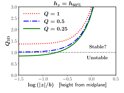
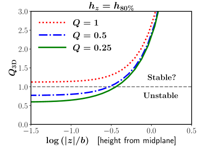
Figure 1: The 3D instability parameter $Q_{\rm 3D}$ as a function of height from the midplane $|z|$ for a rotating, self-gravitating stratified disc in vertical isothermal equilibrium (Equation 20) at a given radius, for different values of Toomre’s 2D instability parameter $Q$. $Q_{\rm 3D}$ is calculated for $\gamma=5/3$ and either $h_{z}=h_{60\%}$ (thickness containing 60% of the mass per unit surface; left panel) or $h_{z}=h_{80\%}$ (thickness containing 80% of the mass per unit surface; right panel). Our sufficient 3D instability criterion predicts instability where $Q_{\rm 3D}<1$, but does not guarantee stability where $Q_{\rm 3D}>1$.

Using Equations (20-22) and $\rho_{0}=\pi G\Sigma^{2}/(2c_{\rm s,iso}^{2})$, where

$$\Sigma=\int_{-\infty}^{\infty}\rho(z){\rm d}z$$ (23)

is the surface density, for the isothermal disc the sufficient condition for instability (16) becomes

$$Q_{\rm 3D}=\sqrt{\frac{Q^{2}}{2}\cosh^{2}\tilde{z}+2\sinh^{2}\tilde{z}}+\sqrt{\frac{5}{6}}\frac{b}{h_{z}}\cosh\tilde{z}<1\qquad\mbox{(sufficient for instability)},$$ (24)

where

$$Q\equiv\frac{\kappa c_{\rm s,iso}}{\pi G\Sigma}$$ (25)

is the classical 2D Toomre (1964) instability parameter at a given radius. Fig. 1 shows $Q_{\rm 3D}$ as a function of $z$ for representative values of $Q$ when $h_{z}=h_{60\%}\simeq 1.4b$ (left panel) and $h_{z}=h_{80\%}\simeq 2.2b$ (right panel), which should bracket realistic values of $h_{z}$ (see Section 4.1.2 and Appendix C). $Q_{\rm 3D}$ is an increasing function of $|z|$, so, at given radius, the disc is more prone to gravitational instability near the midplane. For both choices of $h_{z}$ the $Q=1$ model is stable and the $Q=0.25$ model is unstable; the $Q=0.5$ model is marginally stable for $h_{z}=h_{60\%}$ and unstable for $h_{z}=h_{80\%}$. The overall condition to have instability at any height at a given radius in the considered stratified disc is $Q_{\rm 3D,min}=Q_{\rm 3D}(0)<1$, i.e.

$$Q<Q_{\rm crit}=\sqrt{2}-\sqrt{\frac{5}{3}}\frac{b}{h_{z}}\qquad\mbox{(sufficient for instability)},$$ (26)

which gives $Q_{\rm crit}\simeq 0.48$ for $h_{z}=h_{60\%}$ and $Q_{\rm crit}\simeq 0.83$ for $h_{z}=h_{80\%}$, broadly consistent with Toomre’s 2D criterion $Q<1$, given the known stabilizing effect of finite thickness (see Section 5.3).

When the conditions for instability are met, there is a range of unstable radial wavenumbers (satisfying inequality 17) centred at $|k_{R}|=k_{R,{\rm inst}}$ (see Appendix B.3). For the discs here considered $k_{R,{\rm inst}}$ is largest in the midplane, where it can be written as

$$k_{R,{\rm inst}}^{2}h_{z}^{2}=\frac{3}{5}\frac{h_{z}^{2}}{b^{2}}\left(1-\frac{Q^{2}}{2}\right)-\frac{1}{2},$$ (27)

which gives $0.7\lesssim k_{R,{\rm inst}}h_{z}\lesssim 1.5$ for $h_{60\%}\lesssim h_{z}\lesssim h_{80\%}$ and $0\lesssim Q\lesssim Q_{\rm crit}$. Thus, the typical unstable modes ($|k_{R}|h_{z}\approx 1$) have radial wavelength $\approx 2\pi h_{z}$, consistent with estimates obtained in finite thickness-corrected 2D models (Kim et al. 2002; Romeo & Agertz 2014; Behrendt et al. 2015; see Section 5.3). We note that, provided that $h_{z}$ is smaller than $R$, $k_{R,{\rm inst}}$ is larger than $1/R$, consistent with our assumptions.

5.2 Sufficient criterion for stability

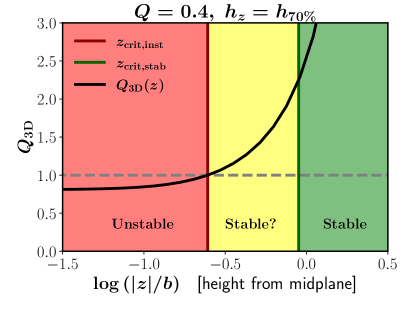
Figure 2: Instability and stability regions as a function of height from the midplane $|z|$ at a given radius for a rotating, self-gravitating stratified disc in vertical isothermal equilibrium (Equation 20) with 2D Toomre’s parameter $Q=0.4$ for $\gamma=5/3$. The instability region ($|z|<z_{\rm crit,inst}$; red) is determined by the criterion $Q_{\rm 3D}<1$ (Equation 24) with $h_{z}=h_{70\%}$. The stability region ($|z|>z_{\rm crit,stab}$; green) is determined by the condition (28). In the yellow region stability is not guaranteed by our criteria.

Combining Equation (12) with Equations (21) and (22), we get that for the isothermal stratified disc a sufficient condition for stability is

$$\frac{4}{3\cosh^{2}\tilde{z}}\left(\frac{6}{5}\sinh^{2}\tilde{z}-1\right)>Q^{2}\qquad\mbox{(sufficient for stability)}.$$ (28)

The l.h.s. of this inequality is an increasing function of $|z|$. When $Q\lesssim 1.27$ this sufficient criterion guarantees stability at $|z|>z_{\rm crit,stab}$, where $z_{\rm crit,stab}>b\operatorname{asinh}{\sqrt{5/6}}\simeq 0.82b$ is an increasing function of $Q$.

Fig. 2 shows, for a representative isothermal disc with $Q=0.4$ at a given radius, stability and instability regions, as a function of height from midplane, obtained combining our sufficient criteria for stability (Equation 28) and instability (Equation 24), taking for the latter as fiducial value $h_{z}=h_{70\%}\simeq 1.7b$, such that $Q_{\rm crit}\simeq 0.67$ (Equation 26). The disc is unstable close to the midplane (at $|z|<z_{\rm crit,inst}\simeq 0.25b$) and stable at $|z|>z_{\rm crit,stab}\simeq 0.9b$, while stability is not guaranteed at intermediate heights.

5.3 Comparison with finite-thickness corrected 2D models

Here we compare our results on the isothermal disc with those obtained with modifications of the thin-disc stability criteria that account for finite thickness, which, as mentioned in Section 1, is a complementary approach to study the local gravitational instability in realistically thick discs. These modified 2D criteria are based on 2D models in which the self-gravity of the perturbation is corrected with a reduction factor $\mathcal{F}$, depending both on the radial wavenumber of the perturbation and on the disc scale height $h$. Different authors have adopted different functional forms of $\mathcal{F}$, but, for given $\mathcal{F}$, by computing the wavenumber of the most unstable mode, it is always possible to express the condition for instability as $Q<Q_{\rm crit}$, where $Q_{\rm crit}$ depends on the unperturbed vertical density distribution. Focusing on the self-gravitating isothermal disc, we can thus compare the values of $Q_{\rm crit}$ that we find using our 3D criterion ($Q_{\rm crit}\simeq 0.5,\,0.7$ and $0.8$ for $h_{z}=h_{60\%},\,h_{70\%}$ and $h_{80\%}$, respectively; see Sections 5.1 and 5.2), with those obtained in the literature using modified 2D criteria: $Q_{\rm crit}\simeq 0.65$ (Kim et al., 2002), $0.6\lesssim Q_{\rm crit}\lesssim 0.65$ (Bertin & Amorisco 2010, considering two different functional forms of $\mathcal{F}$; see also Bertin 2014), $Q_{\rm crit}\simeq 0.69$ (Wang et al., 2010), $Q_{\rm crit}\simeq 0.67$ (Romeo & Falstad 2013, based on the calculations presented in Romeo 1992) and $Q_{\rm crit}\simeq 0.70$ (Behrendt et al., 2015). These values of $Q_{\rm crit}$ are consistent with those found with our 3D criterion, with a remarkably good agreement when $h_{z}\approx h_{70\%}$.

6 Conclusions

In this letter we have derived dispersion relations for axisymmetric perturbations, which can be used to study the local gravitational stability in stratified rotating axisymmetric gaseous systems with general baroclinic (Equation 3) and barotropic (Equation 7) distributions, as well as in vertically stratified discs (Equations 9, 13 and 15). We have obtained 3D sufficient stability (Equation 12) and instability (Equations 16 and 19) criteria, which generalize previous results and can be used to determine whether and where a rotating system of given 3D structure is prone to fragmentation and clump formation.

In the case of vertically stratified discs, we have expressed the sufficient instability criterion as $Q_{\rm 3D}<1$ (Equation 16), where the dimensionless parameter $Q_{\rm 3D}=\left(\sqrt{\kappa^{2}+\nu^{2}}+c_{\rm s}h_{z}^{-1}\right)/{\sqrt{4\pi G\rho}}$ can be seen as a 3D version of Toomre’s 2D $Q$ parameter, in which the combined stabilizing effects of rotation ($\kappa^{2}$) and stratification ($\nu^{2}$) are apparent. A shortcoming of this 3D criterion is that the disc thickness parameter $h_{z}$ is not exactly defined. However, the comparison with previous 2D and 3D models in the literature (Section 5 and Appendix C) suggests to use as fiducial value $h_{z}\approx h_{70\%}$, where $h_{70\%}$ is the height of a strip centred on the midplane containing 70% of the mass per unit surface. Independent of the specific assumed definition of $h_{z}$, applying our criteria to discs with isothermal vertical stratification, we have shown quantitatively that the conditions for gravitational instability are more easily met close to the midplane, while stability prevails far from the midplane. In the midplane of unstable discs, the typical perturbations that are expected to grow have radial extent of a few $h_{z}$.

When the conditions for gravitational instability are satisfied, the perturbations are expected to grow and enter the non-linear regime, which cannot be studied using the linearized equations considered in this work. Though numerical simulations would be necessary to describe quantitatively the non-linear growth of axisymmetric disturbances, qualitatively we expect that the outcome of the instability would be the formation of thick ring-like structures in the equatorial plane of the rotating gaseous systems, which might then fragment into spiral arms, filaments and clumps (see Wang et al., 2010; Behrendt et al., 2015). These clumps are likely to be the sites of star formation in galactic discs and possibly of planet formation in protostellar discs. Collapsed overdense rings are not expected to form out of the midplane, not only because there the instability conditions are harder to meet (see Figs 1 and 2), but also because in the vertical direction the gravitational instability is essentially Jeans-like with Jeans length is of the order of the vertical scale-height (see Section 4.1.1 and Appendix A), so there is no room to form vertically distinct rings. The 3D structure of filaments formed in the midplane of gravitationally unstable plane-parallel stratified non-rotating systems has been studied with hydrodynamic simulations by Van Loo et al. (2014, see their figures 6 and 7). Mutatis mutandis, the results of Van Loo et al. (2014) suggest that, in an unstable rotating stratified disc, the collapsed overdense rings will likely have vertical density distributions similar in shape to that of the unperturbed disc, but with smaller scaleheight.

Data Availability

The data underlying this article will be shared on reasonable request to the corresponding author.

Appendix A Restrictions on the perturbation wavenumber

For the perturbation analysis to be consistent, the size of the disturbance must be smaller than the characteristic length scales of the unperturbed system. In particular, the properties of the background must not vary significantly over the size of the perturbations, so we must exclude from our analysis perturbations with $k$ smaller than $1/\ell$, where $\ell\equiv|q|/||{\nabla}q||$ is the characteristic length over which any quantity $q$ varies in the unperturbed configuration at the position of the disturbance. An estimate of $1/\ell^{2}$ is $||{\nabla}\rho||||{\nabla}p||/(\rho p)$. In general, in the presence of rotation, the vertical density and pressure gradients are stronger than the corresponding radial gradients, so we can take $1/\ell^{2}\approx|\rho^{\prime}_{z}p^{\prime}_{z}|/(\rho p)$. Of course, the underlying assumption is that the unperturbed gas distribution is sufficiently smooth, so that $\ell$ can give a measure of macroscopic gradients and is not affected by small-scale inhomogeneities.

As an additional restriction on the perturbation wavenumber, we also require $k$ to be larger than $1/\mathcal{L}$, where $\mathcal{L}$ is the macroscopic length scale of the gaseous system. In order to estimate $\mathcal{L}$, let us consider a very general argument (e.g. Binney & Tremaine, 2008; Bertin, 2014): it follows from the virial theorem that an equilibrium self-gravitating gaseous system of mass $M$ and sound speed $c_{\rm s}$ has characteristic size $\mathcal{L}\approx GM/c_{\rm s}^{2}$. This equation, combined with $M\approx\rho\mathcal{L}^{3}$, where $\rho$ is the mean density of the system, gives $1/\mathcal{L}^{2}\approx G\rho/c_{\rm s}^{2}\approx k_{\rm J}^{2}$, where $k_{\rm J}^{2}=4\pi G\rho/c_{\rm s}^{2}$ is the Jeans wavenumber squared. So the characteristic size of a self-gravitating gaseous system is of the order of the Jeans length. This has the sometime overlooked implication that, in the case of a gas cloud of finite size, the classical Jeans stability analysis proves that linear perturbations with $k\gtrsim k_{\rm J}$ are stable, but does not prove that modes with $k\lesssim k_{\rm J}$ are unstable. For a rotating flattened system the shortest macroscopic scale is the vertical scale height, which is typically of the order $1/k_{\rm J}$ (see e.g. the case of a vertical isothermal distribution; Section 5).

The above simple arguments indicate that we must exclude from our analysis modes with $k^{2}\lesssim|\rho^{\prime}_{z}p^{\prime}_{z}|/(\rho p)$ and modes with $k\lesssim k_{\rm J}$. In practice, to approximately implement both these conditions, we find it convenient to limit our analysis to modes with $k$ satisfying Equation (11). This restriction is adopted throughout Section 4, with the only exception of Section 4.1.2.

Appendix B Analysis of the dispersion relations

In this Appendix we analyze dispersion relations in the form $P(\omega,s)=0$, where $\omega$ is the frequency and $s\equiv c_{\rm s}^{2}k^{2}$ with $k$ the wavenumber, which are biquadratic in $\omega$. For given $s$, we indicate the zeros of $P$ as $\omega^{2}_{1}$ and $\omega^{2}_{2}>\omega^{2}_{1}$, and the discriminant of $P$ as $\Delta_{\omega}$. In the analysis, when dealing with a quadratic polynomial of $s$, we indicate its discriminant as $\Delta_{s}$ and its zeros as $s_{1}$ and $s_{2}>s_{1}$. When $\omega^{2}$ is real, the condition for stability is $\omega^{2}_{1}>0$. Modes such that $\omega^{2}$ is not real are unstable (overstable), because there is at least one solution with positive ${\rm Im}(\omega)$.

To simplify the notation we define the positive quantities $A\equiv 4\pi G\rho$, $B\equiv\kappa^{2}$, $C\equiv\nu^{2}$, $D\equiv N_{z}^{2}$ and $E\equiv c_{\rm s}^{2}h_{z}^{-2}$, all with dimensions of a frequency squared, as well as the dimensionless quantity $\zeta\equiv k_{z}^{2}/k^{2}$, which is a measure of the relative contribution of the vertical component of the wavevector. The coefficients of the dispersion relations depend in general on $A$, $B$, $C$, $D$, $E$ and $\zeta$. By definition $0\leq\zeta\leq 1$; we further assume $A>0$, $B>0$, $C>0$, $D>0$ and $E>0$ (see Section 4). We recall that $C>D$ (see Equation 10) and that in all the following sections, with the only exception of Section B.3, we limit our analysis to modes with $s>A+C$ (see Equation 11).

B.1 Dispersion relations in the form ’ABCD$\zeta$’

We consider here dispersion relations in the form

$$\omega^{4}+(A-B-C-s)\omega^{2}+(1-\zeta)Ds+\zeta Bs-\zeta AB+BC=0.$$ (29)

The discriminant of the dispersion relation is

$$\begin{split}\Delta_{\omega}&=(A-B-C-s)^{2}-4(1-\zeta)Ds-4\zeta Bs+4\zeta AB-4BC\\ &=s^{2}-2\left[A-B-C+2(1-\zeta)D+2\zeta B\right]s+(A-B-C)^{2}+4\zeta AB-4BC,\end{split}$$ (30)

which is positive for $s\to\infty$. The discriminant of $\Delta_{\omega}(s)$ is

$$\begin{split}\Delta_{s}&=4[A-B-C+2(1-\zeta)D+2\zeta B]^{2}-4(A-B-C)^{2}-16\zeta AB+16BC\\ &=16(1-\zeta)\left[(A-B-C+D)D+BC-\zeta(B-D)^{2}\right].\end{split}$$ (31)

$\omega_{1}^{2}$ is given by

$$2\omega_{1}^{2}=s-(A-B-C)-\sqrt{\Delta_{\omega}}.$$ (32)

When $\Delta_{\omega}>0$, given that $s>A+C>A-B-C$, the condition for stability $\omega_{1}^{2}>0$ can be written as

$$s>\frac{A-\zeta^{-1}C}{1+\zeta^{-1}(1-\zeta)(D/B)},$$ (33)

which is always satisfied. It follows that there is never monotonic instability.

When $(A-B-C+D)D+BC<0$, i.e.

$$AD<(C-D)(D-B)\qquad\mbox{(sufficient for stability)}$$ (34)

$\Delta_{s}<0$ (and thus $\Delta_{\omega}>0$) $\forall\zeta$. Thus inequality (34) is a sufficient condition for stability.

B.2 Dispersion relations in the form ’ABC’

We consider here dispersion relations in the form

$$\omega^{4}+(A-B-C-s)\omega^{2}+Bs-AB+BC=0.$$ (35)

The discriminant of the dispersion relation is

$$\Delta_{\omega}=(A-B-C-s)^{2}-4Bs+4AB-4BC=[s-(A+B-C)]^{2}\geq 0,$$ (36)

so $\omega^{2}$ is always real. For stability $\omega_{1}^{2}>0$ i.e. $s-(A-B-C)-\sqrt{[s-(A+B-C)]^{2}}>0$, which, for $s>A+C>A-B-C$ becomes $[s-(A-B-C)]^{2}>[s-(A+B-C)]^{2}>0$. If $s>(A+B-C)$ the latter inequality reduces to $B>0$, which is always satisfied; if $s<A+B-C$ it reduces to $s>A+C$, which is always satisfied. Thus all modes are stable.

B.3 Dispersion relations in the form ’ABCDE’

We consider here dispersion relations in the form

$$\omega^{4}+\left(\frac{As}{s+E}-B-C-s\right)\omega^{2}+Ds+BC=0,$$ (37)

with $C>D$. Different from the rest of Appendix B, here we consider also modes with $s<A+C$. The discriminant of the dispersion relation is

$$\Delta_{\omega}=\left(A\frac{s}{s+E}-B-C-s\right)^{2}-4Ds-4BC,$$ (38)

whose sign is determined by the sign of a third order polynomial in $s$. However, we can derive useful instability conditions even without determining the sign of $\Delta_{\omega}$. When $\Delta_{\omega}<0$ we have overstability. When $\Delta_{\omega}>0$, the condition to have monotonic instability is $\omega_{1}^{2}<0$, i.e.

$$-g(s)<\sqrt{g^{2}(s)-4Ds-4BC},$$ (39)

where

$$g(s)\equiv A\frac{s}{s+E}-B-C-s.$$ (40)

The inequality is satisfied only when $g(s)>0$. Thus, if $g(s)>0$ and $\Delta_{\omega}>0$ we have monotonic instability. If $g(s)>0$ and $\Delta_{\omega}<0$ we have overstability. This implies that a sufficient condition for instability is $g(s)>0$, i.e.

$$s^{2}-(A-B-C-E)s+E(B+C)<0\qquad\mbox{(sufficient for instability)},$$ (41)

whose discriminant is $\Delta_{s}=A^{2}-2(B+C+E)A+(B+C-E)^{2}$. The larger root $s_{2}$ of the polynomial is given by $2s_{2}=A-B-C-E+\sqrt{\Delta_{s}}$. We have instability when $\Delta s>0$ and $s_{2}>0$. Imposing these two conditions we get

$$\frac{\sqrt{B+C}+\sqrt{E}}{\sqrt{A}}<1\qquad\mbox{(sufficient for instability)},$$ (42)

which is thus a sufficient condition for instability. We note that, when combined with $s_{2}>0$, $\Delta s>0$ implies $s_{1}>0$: the interval of unstable wavenumbers $s_{1}<s<s_{2}$ is centred at $(A-B-C-E)/2>\sqrt{E(B+C)}$.

B.4 Dispersion relations in the form ’ABCD’

We consider here dispersion relations in the form

$$\omega^{4}+(A-B-C-s)\omega^{2}+Ds+BC=0,$$ (43)

with $C>D$. The discriminant of the dispersion relation is

$$\Delta_{\omega}=(A-B-C-s)^{2}-4Ds-4BC=s^{2}-2(A-B-C+2D)s+(A-B-C)^{2}-4BC.$$ (44)

The discriminant of $\Delta_{\omega}(s)$ is

$$\Delta_{s}=4(A-B-C+2D)^{2}-4(A-B-C)^{2}+16BC=16[(A-B-C+D)D+BC].$$ (45)

When $\Delta_{\omega}>0$, the condition for instability $\omega_{1}^{2}<0$ gives $Ds+BC<0$, which is never satisfied, so there is no monotonic instability. The conditions to have overstability are $\Delta_{s}>0$ and $s_{2}>A+C$. Given that $s_{2}=A-B-C+2D+s\sqrt{(A-B-C+2D)D+BC}$, these conditions jointly lead to

$$AD>C(C-D)+(B/2)^{2}\qquad\mbox{(sufficient for instability)}.$$ (46)

When this condition is satisfied there are unstable (overstable) modes.

Appendix C Comparison with criteria for vertically stratified discs with polytropic equation of state

In order to gauge the disc thickness parameter $h_{z}$ appearing in our instability criterion (16) for vertically stratified discs, here we compare our criterion with those found by Goldreich & Lynden-Bell (1965a) for uniformly rotating self-gravitating discs with polytropic equation of state $p\propto\rho^{{{\gamma^{\prime}}}}$, considering in particular values of the polytropic index ${{\gamma^{\prime}}}=1$ and ${{\gamma^{\prime}}}=2$. Our linear stability analysis, performed for adiabatic perturbations, can be adapted to the case of a polytropic equation of state simply imposing $\gamma={{\gamma^{\prime}}}$, when the unperturbed distribution is stratified with $p\propto\rho^{{\gamma^{\prime}}}$. As a measure of the thickness $h_{z}$ we can take the height $h_{X\%}$ of a strip centred on the midplane containing a fraction $\xi=0.01X$ of the mass per unit surface: $h_{X\%}=2z_{\xi}$, with $z_{\xi}$ such that

$$\frac{1}{\Sigma}\int_{-z_{\xi}}^{z_{\xi}}\rho(z){\rm d}z=\xi,$$ (47)

where $\Sigma$ is given by Equation (23). The following analysis of the ${{\gamma^{\prime}}}=1$ (Section C.1) and ${{\gamma^{\prime}}}=2$ (Section C.2) cases suggests that a good range of values of $h_{z}$ should be $h_{60\%}\lesssim h_{z}\lesssim h_{80\%}$.

C.1 Self-gravitating isothermal disc with equation of state $p\propto\rho$

In the case of an isothermal disc, the vertical density distribution is $\rho(z)=\rho_{0}{\rm sech}^{2}(z/b)$, where $\rho_{0}=\rho(0)$ and $b=c_{\rm s,iso}/\sqrt{2\pi G\rho_{0}}$ (Spitzer 1942; see also Section 5), so

$$h_{X\%}=2b\operatorname{atanh}\xi.$$ (48)

Goldreich & Lynden-Bell (1965a) found that a uniformly rotating ($\kappa^{2}=4\Omega^{2}$), self-gravitating isothermal disc is unstable against isothermal perturbations when $\pi G\bar{\rho}/\kappa^{2}>0.73$, where

$$\bar{\rho}\equiv\frac{1}{\Sigma}\int_{-\infty}^{\infty}\rho^{2}(z){\rm d}z=\frac{2}{3}\rho_{0}$$ (49)

is the mean gas density. It is straightforward to show that for this disc model, at given radius, the parameter $Q_{\rm 3D}(z)$ defined in Equation (16) attains its minimum at $z=0$, so a sufficient condition to have instability at any height in the disc at the considered radius is $Q_{\rm 3D,min}=Q_{\rm 3D}(0)<1$. For this model, imposing $\gamma=1$, the instability condition $Q_{\rm 3D,min}<1$ can be rewritten as

$$\frac{\pi G\bar{\rho}}{\kappa^{2}}>\frac{1}{6}\left(1-\frac{1}{\sqrt{2}}\frac{b}{h_{z}}\right)^{-2}\qquad\mbox{(sufficient for instability)}.$$ (50)

Using $h_{z}=h_{X\%}$ and Equation (48), the r.h.s. of the above equation equals 0.73 for $\xi\simeq 0.59$, i.e. $h_{z}\approx h_{60\%}$.

C.2 Self-gravitating polytropic disc with equation of state $p\propto\rho^{2}$

In this case the vertical density distribution is given by (Goldreich & Lynden-Bell, 1965a)

$$\rho(z)=\rho_{0}\cos\left(\frac{\pi}{2}\frac{z}{a}\right),$$ (51)

for $|z|\leq a$ and $\rho=0$ for $|z|>a$, where $\rho_{0}=\rho(0)$ is the density in the midplane, $a=\sqrt{\pi}c_{\rm s,0}/(4\sqrt{G\rho_{0}})$ is a characteristic scale length and $c_{\rm s,0}=\sqrt{2p_{0}/\rho_{0}}$ is the sound speed at $z=0$ with $p_{0}$ the pressure in the midplane. For this model $\bar{\rho}=(\pi/4)\rho_{0}$ and

$$h_{X\%}=\frac{4a}{\pi}\arcsin\xi.$$ (52)

Goldreich & Lynden-Bell (1965a) found that this model is unstable against polytropic ${{\gamma^{\prime}}}=2$ perturbations when $\pi G\bar{\rho}/\kappa^{2}>1.11$. As for the isothermal disc (Section C.1), also in this case the condition to have instability at any height at a given radius in the disc is $Q_{\rm 3D,min}=Q_{\rm 3D}(0)<1$, which, imposing $\gamma=2$, can be rewritten as

$$\frac{\pi G\bar{\rho}}{\kappa^{2}}>\frac{\pi}{16}\left(1-\frac{2}{\pi}\frac{a}{h_{z}}\right)^{-2}\qquad\mbox{(sufficient for instability)}.$$ (53)

Using $h_{z}=h_{X\%}$ and Equation (52), the r.h.s. of the above inequality equals 1.11 for $\xi\simeq 0.76$, i.e. $h_{z}\approx h_{80\%}$.

References

- Bacchini et al. (2019) Bacchini C., Fraternali F., Pezzulli G., Marasco A., Iorio G., Nipoti C., 2019, A&A, 632, A127
- Balbus (1995) Balbus S. A., 1995, ApJ, 453, 380
- Behrendt et al. (2015) Behrendt M., Burkert A., Schartmann M., 2015, MNRAS, 448, 1007
- Bertin (2014) Bertin G., 2014, Dynamics of Galaxies. Cambridge University Press
- Bertin & Amorisco (2010) Bertin G., Amorisco N. C., 2010, A&A, 512, A17
- Bertin & Casertano (1982) Bertin G., Casertano S., 1982, A&A, 106, 274
- Binney & Tremaine (2008) Binney J., Tremaine S., 2008, Galactic Dynamics: Second Edition. Princeton University Press
- Chandrasekhar (1961) Chandrasekhar S., 1961, Hydrodynamic and hydromagnetic stability. Clarendon Press: Oxford University Press
- Cimatti et al. (2019) Cimatti A., Fraternali F., Nipoti C., 2019, Introduction to galaxy formation and evolution: from primordial gas to present-day galaxies. Cambridge University Press
- Elmegreen (2011) Elmegreen B. G., 2011, ApJ, 737, 10
- Förster Schreiber et al. (2006) Förster Schreiber N. M., et al., 2006, ApJ, 645, 1062
- Genkin & Safronov (1975) Genkin I. L., Safronov V. S., 1975, Soviet Ast., 19, 189