Detecting planetary mass companions near the water frost-line using
JWST interferometry
Abstract
JWST promises to be the most versatile infrared observatory for the next two decades. The Near Infrared and Slitless Spectrograph (NIRISS) instrument, when used in the Aperture Masking Interferometry (AMI) mode, will provide an unparalleled combination of angular resolution and sensitivity compared to any existing observatory at mid-infrared wavelengths. Using simulated observations in conjunction with evolutionary models, we present the capability of this mode to image planetary mass companions around nearby stars at small orbital separations near the circumstellar water frost-line for members of the young, kinematic moving groups Pictoris, TW Hydrae, as well as the Taurus-Auriga association. We show that for appropriately chosen stars, JWST/NIRISS operating in the AMI mode can image sub-Jupiter companions near the water frost-lines with confidence. Among these, M-type stars are the most promising. We also show that this JWST mode will improve the minimum inner working angle by as much as in most cases when compared to the survey results from the best ground-based exoplanet direct imaging facilities (e.g. VLT/SPHERE). We also discuss how the NIRISS/AMI mode will be especially powerful for the mid-infrared characterization the numerous exoplanets expected to be revealed by Gaia. When combined with dynamical masses from Gaia, such measurements will provide a much more robust characterization of the initial entropies of these young planets, thereby placing powerful constraints on their early thermal histories.
keywords:
techniques: interferometric – instrumentation: high angular resolution – exoplanets – planets and satellites: detection – methods: statistical1 Introduction
High contrast imaging of nearby circumstellar environments is the only technique that provides sensitivity to planetary mass companions (PMCs hereon) at wide orbital separations (e.g. Bowler, 2016), and hence will extensively map out the outer architectures of planetary systems through the coming years with the advent of next generation telescopes. Previous efforts have led to successful detection of wide-separation PMCs (e.g. Marois et al., 2008; Lagrange et al., 2009; Chauvin et al., 2017; Bohn et al., 2020) and numerous scattered-light images of disks (e.g. Matthews et al., 2017; Milli et al., 2017; Esposito et al., 2020; Hinkley et al., 2021). Since this technique preferentially observes young stars, it is also exceptionally well-positioned to place valuable constraints on competing models of planet formation and migration that describe the early dynamical and thermal evolution of planets (Boley, 2009; Alexander & Armitage, 2009; Marleau & Cumming, 2014; Wallace et al., 2021).
Careful analysis of recent direct imaging (DI, hereon) exoplanet surveys (Nielsen et al., 2019; Wagner et al., 2019; Vigan et al., 2021) indicate that numerous lower mass PMCs exist at wide orbital separations (tens to hundreds of au). Specifically, extrapolating mass distribution power laws derived by the Gemini Planet Imager (GPI hereon) survey (Nielsen et al., 2019) demonstrates that an abundance of planets should be hosted by stars with masses . Microlensing efforts (Poleski et al., 2021) are also consistent with this prediction, providing statistical evidence for the existence of ice giant planets () per star at separations . Detecting an abundance of such companions would be significantly valuable for evaluating the early thermal histories of giant planets, and possibly assigning populations of planets to formation mechanism models based on the accretion of solids in a protoplanetary disk (Pollack et al., 1996) or the formation of a planet triggered by an instability within the disk (e.g. Kratter et al., 2010).
Even with all these remarkable observational accomplishments and the development of state-of-the-art models mapping planet formation histories (e.g., Mordasini et al., 2016, 2017; Mollière et al., 2022), several fundamental questions still remain unanswered. The exact details of the gas-giant planet formation process, as well as the physical and thermodynamic conditions of newly formed planets, remain unclear (Marleau & Cumming, 2014). This is reflected in the fact that models of luminosity evolution of planets vary by orders of magnitude at the youngest ages (Fortney et al., 2008; Spiegel & Burrows, 2012). Early entropy conditions, being the single best route towards enlightening the complex early physics of planet formation (Marleau & Cumming, 2014; Wallace et al., 2021), still remain largely unconstrained. Provided that we can access their orbital locations, obtaining luminosity measurements of numerous young planets with the goal of measuring their entropy will be a major focus for DI searches going forward.
Coronagraphic DI surveys in the last years (e.g. Chauvin et al., 2015; Galicher et al., 2016; Vigan et al., 2017, 2021), have had a low rate of detection of companions around host stars, returning a number of companions that is insufficient to statistically place constraints on planetary formation models as well as models of the early entropy of planets. This poor detection rate of DI planets may be due to the fact that the recent studies (e.g., Fernandes et al., 2019; Fulton et al., 2021) indicate that the peak of the extrasolar giant planet distribution lies at , which coincides well with the water frost lines for solar type stars where planet formation is thought to be more efficient. Theoretical studies (e.g., Frelikh et al., 2019) also point to an increased abundance at this orbital separation.
Due to the fundamental limiting resolution of telescopes at near-infrared wavelengths, recent DI searches (Vigan et al., 2021) can barely reach frost line separations of . Only 20 stars from the first targets of the SHINE coronagraphic survey (Desidera et al., 2021; Langlois et al., 2021; Vigan et al., 2021, consisting of 150 stars) using VLT/SPHERE had the combination of youth and proximity to reach sensitivities of exoplanets at . And less than 5 stars from this survey allowed sensitivities to exoplanets at . This orbital region for nearby stars has been recently accessed on rare occasions, but only via optical interferometry using long-baselines (e.g., Nowak et al., 2020; Hinkley et al., 2022a). But this orbital region is expected to remain largely out-of-reach for ground-based 8-10m telescopes. Even with JWST (Gardner et al., 2006), the Rayleigh diffraction limit ( /D) at wavelength only allows imaging of companions at –18 au for stars within –. In practice, attaining even this resolution is challenging due to the presence of residual scattered starlight not suppressed by the coronagraph, as well as the coronagraphic inner working angle (IWA) itself. In the case of the Near Infrared Camera (Rieke et al., 2005, NIRCam hereon) operating at (with the MASK430R round coronagraph), the IWA is 0.87" (corresponding to orbital separations of for stars at ). Hence to image companions orbiting near the frost-line separations for nearby stars, an additional technique is needed to provide sensitivity at small angular separations.
Aperture Masking Interferometry (‘AMI’ hereon, Baldwin et al., 1986; Haniff et al., 1987; Readhead et al., 1988) achieves just this. This technique involves using an opaque mask with a collection of strategically placed holes, arranged in a way such that the baseline between any two holes samples a unique spatial frequency in the pupil plane. This brings the IWA down to and has been successfully used along with Adaptive Optics (AO) from ground-based observatories (e.g. Tuthill et al., 2000; Lloyd et al., 2006; Monnier et al., 2007; Woodruff et al., 2008; Hinkley et al., 2011; Hinkley et al., 2015). For the first time, JWST is executing this on a space telescope (see §3), taking advantage of the exquisite sensitivity of the Near Infrared Imager and Slitless Spectrograph (Doyon et al., 2012, NIRISS hereon) instrument. In this work we show that JWST operating in the NIRISS/AMI mode will possess the combination of angular resolution, sensitivity and contrast to be able to access planetary mass companions at water frost-line separations around carefully selected nearby stars. This capability of JWST presents the opportunity to detect and characterize a much greater number of extrasolar giant planets and thereby constrain their early thermal histories.
In Section 2 we review the selected sample of stars for this study composed of high-probability members of nearby young stellar associations, followed by the simulations we used for our predictions in section 3. In section 4 we describe the conversion of these simulations to mass sensitivity limits and then subsequently to detection probabilities. In section 5 we describe our calculation of the detection yield of planetary mass companions for these synthetic observations. Our main results are discussed in section 6, and we summarise our conclusions in section 7.
2 Sample Selection
For the purposes of this work, a part of the sample of nearby stars selected was the same as in Carter et al. (2021), which was comprised of the stars in the Pictoris Moving Group (Kastner et al., 1997, Pic hereon) and TW Hydrae Association (Zuckerman et al., 2001, TWA hereon). Although many moving groups consist of stars which provide a combination of age and distance suitable for directly imaging exoplanets (Gagné et al., 2018), Pic and TWA associations satisfy all of the following conditions, making them ideal collections of targets:
For calculations involving the estimation of mass contrast limits using evolutionary models (see section 4.1 for details), the ages used for the stars in the samples of Pic and TWA were and respectively (Malo et al., 2014; Bell et al., 2015).
In addition to Pic and TWA, a list of confirmed members of stars in the Taurus-Auriga Association (Kenyon & Hartmann, 1995, TAA hereon) taken from Kraus et al. (2017) were also used in this analysis. In addition to the significantly younger age of the selected stars, the TAA sample has the advantage of the targets being highly localized on the sky compared to either the TWA or Pic moving groups, which could potentially lead to an enhanced efficiency for a future survey (see §7). There is evidence that the overall stellar population in TAA is comprised of a younger subpopulation of stars with ages of and an older subpopulation with ages as old as (Kraus et al., 2017). To address this issue, the age of each member was calculated using a methodology similar to the one used in Squicciarini et al. (2021), which is detailed in section 5.1. Those stars for which our analysis returned a calculated age were assigned an age of to match the age of that has been well established in previous works on the age of the underlying younger population of stars in TAA. This exercise eradicates any bias in our results from the older population (), and assigning a single age to this younger population ensures that our analysis will be consistent with the single-age methodology we use for the Pic and TWA samples.
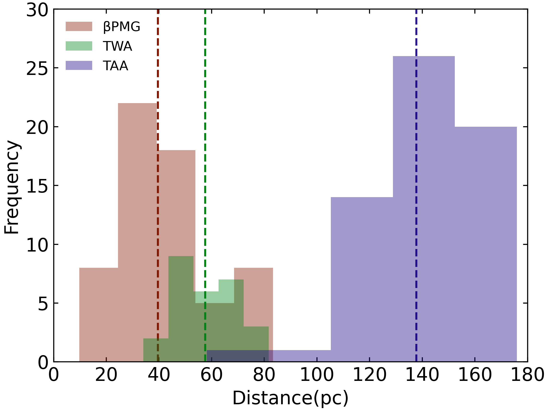
Our final sample contained 150 stars, comprised of 61, 27, and 62 stars from Pic, TWA and TAA respectively (see Figure 1). After selecting the stars for this study, the synthetic contrast curves measuring the sensitivity of the JWST/NIRISS/AMI mode in terms of magnitude, were calculated using existing simulations, as detailed below.
3 NIRISS AMI simulations
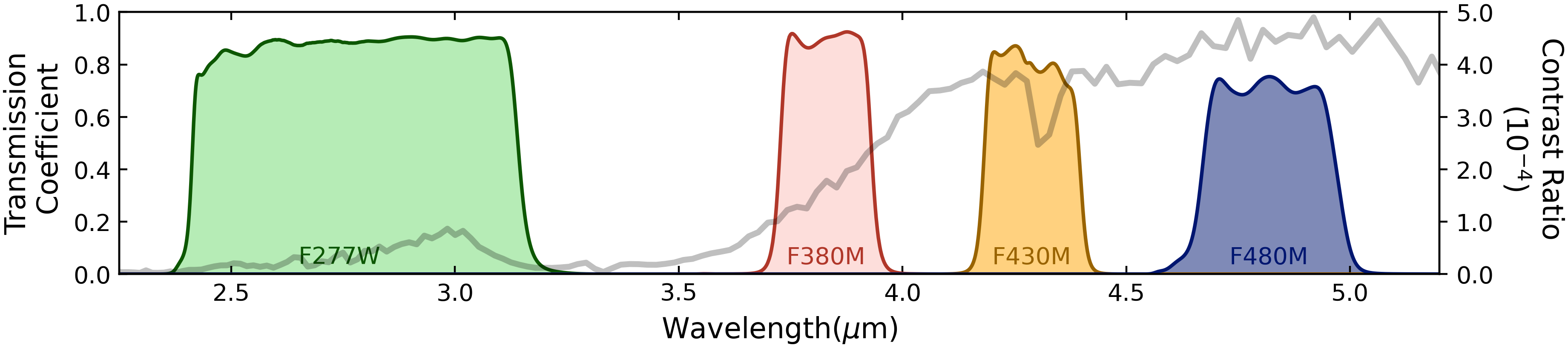
The JWST/NIRISS instrument provides high-contrast interferometric imaging using a non-redundant mask (Sivaramakrishnan et al., 2009), which turns a filled aperture into an interferometric array. This mode offers the possibility of pushing the planet detection parameter space to well within . This mask is an opaque element with 7 hexagonal apertures. These hexagons when projected onto the JWST primary mirror, have an incircle diameter of approximately (Sivaramakrishnan et al., 2012; Greenbaum et al., 2015). Using it in conjunction with the NIRISS filters (F277W, F380M, F430M, and F480M, see Figure 2), this observing mode can probe objects with the highest angular resolution compared to any other mode on JWST (Artigau et al., 2014), and offers the possibility of observing faint targets that would otherwise be inaccessible to ground-based AO facilities.
To detect companions to the stars in the groups of Pic, TWA, and TAA, a desired contrast should be chosen to optimise the potential of making such a discovery. This should then be followed by choosing a particular technique such as AMI or KP interferometry (e.g., Martinache, 2010, “KP” hereon) to execute this. Due to the comparable contrast performance between AMI and KP in the brightness range of the stars considered in this paper, for our analysis we have chosen to utilize the AMI contrast curves as a representative interferometric contrast that can be achieved with JWST. But the actual technique can be chosen later when planning the observations, depending on the brightness of the host star (see §6.4 for more details). To simulate the performance of this mode for particular stars in the moving groups of Pic, TWA, and TAA, the results from Sallum & Skemer (2019) were used which are discussed below.
3.1 Calculating NIRISS AMI contrast curves for a star of any given magnitude
Sallum & Skemer (2019) simulated NIRISS/AMI observations, which were computed using the engine Pandeia (Pontoppidan et al., 2016) and the software WebbPSF (Perrin et al., 2014), both of which are developed using the Python language. Sallum & Skemer (2019) also simulated NIRCam KP observations, which does slightly outperform the AMI observations in certain cases (see §6.4 for more details). In this study we choose to instead focus on the NIRISS/AMI results, which were used to obtain the contrast curves for our study, the methodology for which is explained below.
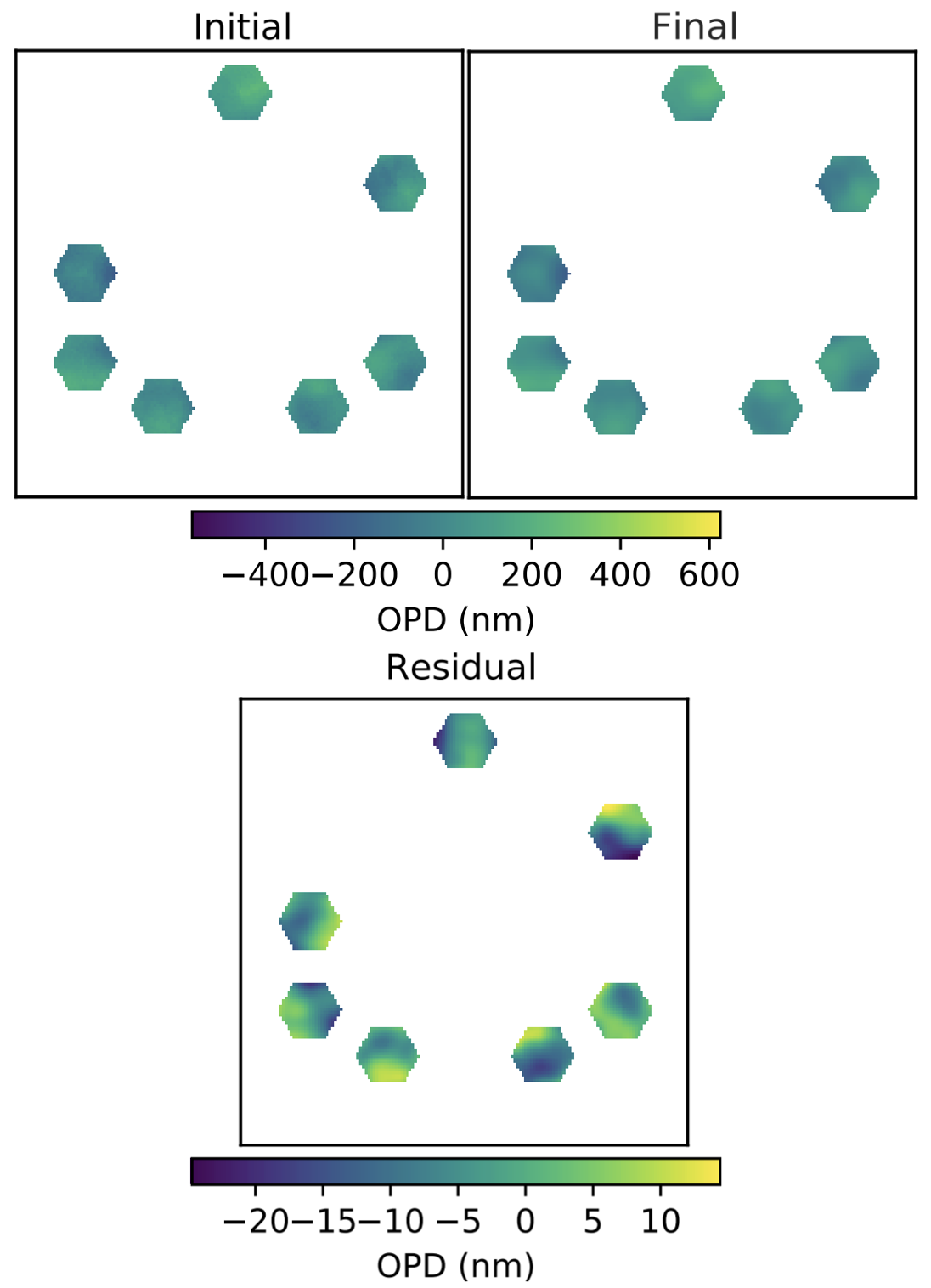
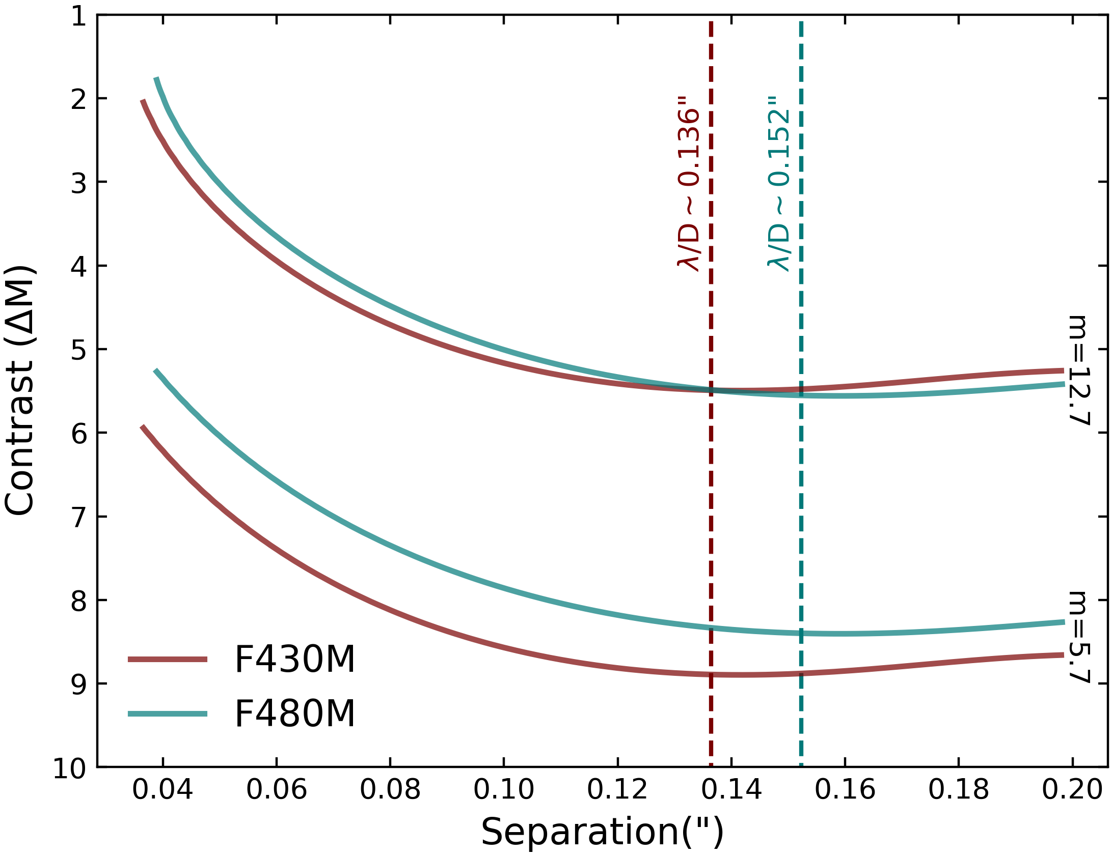
Since exoplanets are relatively bright in the part of the spectrum when compared to their host stars (see Figure 2), the simulations were carried out in filters centred on these wavelengths that can be used with the NIRISS/AMI mode, namely F430M and F480M. These simulated observations were composed of two pairs of target - Point Spread Function (PSF hereon) calibrator visits taken at different telescope roll angles apart, under the assumption that the length of each visit was , and the total observation time was . Although the maximum roll angle for JWST at a given time is , the apart simulated visits do not significantly change the contrast curves, since the fourier coverage of the NIRISS mask is relatively uniform. Thus, the two visits at and respectively should have a similar effect on the ability to recover companions as the two at and , especially since reference PSFs are used (rather than angular differential imaging). As each visit of a JWST observation is split into sets of integrations, which are in turn comprised of a number of groups (Batalha et al., 2017), the maximum number of groups () was calculated that can be used in a single integration without saturation for a star of a given magnitude. Then a visit is constructed with the maximum number of such integrations () that can be acquired in , noting that each integration comes with a readout overhead of (in a sub80 subarray, JDox Project Team, 2016). When the remaining time after integrations allowed for more than a single group, an additional integration containing groups was added. A list containing the values of , and for each calculated magnitude in the F430M and F480M is provided in Table 2 in the appendix, which is recreated from similar tables in Sallum & Skemer (2019). Using the image for the entire visit, science target and calibrator frames were generated using different optical path difference (OPD) maps from WebbPSF. This was followed by fitting a hexike (hexagonal version of zernike, Upton & Ellerbroek, 2004) basis to each mirror segment with 100 coefficients. Finally, each hexike coefficient () is evolved by a factor drawn from a one-mean uniform distribution of width tuned to result in a root mean square residual wave front error of with OPD evolution (see Figure 3), shown in the following equation,
| (1) |
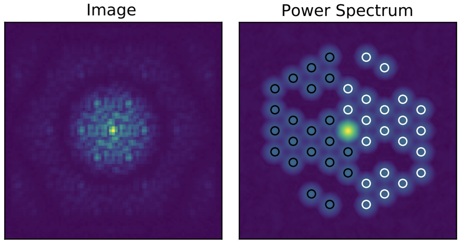
where (for NIRISS) and the calculation is consistent with thermal evolution expected over hour long timescales for JWST. Using these, the simulated images were computed (see Figure 4) from which the contrast curves were extracted.
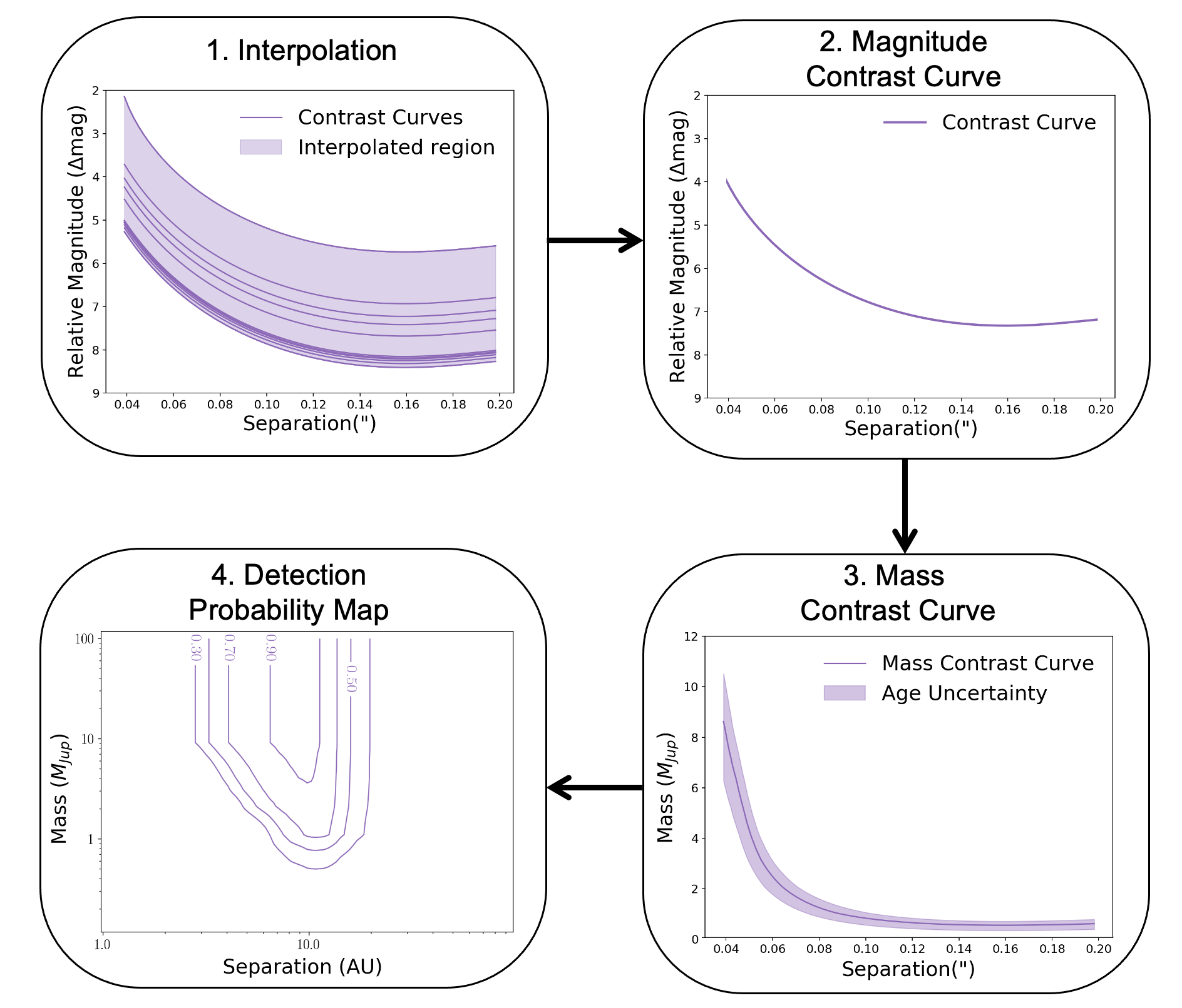
The contrast curves were hence available for stellar apparent magnitude values ranging from 5.7 to 12.7 with increments of 0.1 (see Figure 5). This discrete parameter space was made continuous by interpolating across relative magnitude values for each of the apparent magnitudes values (see Figure 6). This allowed us to compute the filter-specific contrast curve of all the stars in our sample given their apparent magnitude value. These filter-specific stellar apparent magnitude values for stars were calculated using stellar isochronal models and is detailed in the following section.
3.2 Calculating magnitudes of stars in particular filters
Apparent stellar magnitudes in the JWST/NIRISS/AMI filters of F480M and F430M for the stars in our samples of Pic and TWA were calculated following a similar methodology as that described in Carter et al. (2021), which is briefly outlined here for clarity. To begin, the effective temperature () and log() was estimated for each star in the sample by matching their Gaia (Gaia Collaboration et al., 2016, 2018) colours to the theoretical stellar isochrones covering (Baraffe et al., 2015) and (Haemmerlé et al., 2019). A spectral energy distribution (SED) for each star was then determined by matching its estimated and log() to interpolated solar metallicity spectra obtained from Baraffe et al. (2015). These spectra were then normalised using the respective magnitudes of the corresponding star’s WISE () bandpass (Wright et al., 2010; Cutri et al., 2021). Finally, the apparent magnitudes for each star in the NIRISS/AMI filters were calculated using the pysynphot Python package (STScI Development Team, 2013).
For the stars in TAA, given their young age, only the isochrones from Baraffe et al. (2015) were used since these models have a lower age limit of . However, some of the stars in the sample do not have Gaia - colour magnitude values in the domain of these isochrones. To solve this, the filter specific magnitudes ( and ) for the stars which did have - colour magnitude values in the domain were first calculated using the same method as the stars in Pic and TWA. The magnitudes of the remaining stars were calculated from an interpolation of versus magnitudes and vs. magnitudes separately, by reading off their respective magnitudes.
Using these apparent magnitudes, the contrast curves (representing the achieved sensitivity to faint companions, measured in magnitudes fainter than the host star) were computed for each star in the sample using the generated interpolated parameter space as discussed in section 3.1. These contrast curves were then converted into values in terms of mass using the evolutionary models described in Phillips et al. (2020), as detailed in the following section (see Figure 6).
4 Calculation of Detection Probabilities
In this section we describe our calculations of the probability of detecting substellar companions as a function of mass and orbital separation for each of the targets within our sample.
4.1 Mass sensitivity limits
ATMO 2020 is a set of 1D radiative-convective equilibrium cloudless models describing the atmosphere and evolution of cool brown dwarfs and self-luminous giant exoplanets (Phillips et al., 2020), spanning the mass range of . This set of models was used to convert the obtained contrast curves to mass sensitivity limits at given separations. ATMO offers three different sets of evolutionary models: one at chemical equilibrium, and the other two at chemical disequilibrium assuming different strengths of vertical mixing. We keep our calculations and results limited to the case of equilibrium models, since this case provides the baseline scenario of planetary atmospheric conditions, eliminating more complex considerations related to atmospheric dynamics, such as vertical atmospheric mixing (Barman et al., 2011; Konopacky et al., 2013). Although some planetary mass companions do show signs of disequilibrium chemistry, for simplicity this study does not take disequilibrium models into consideration. Using these mass sensitivity limits hence calculated for each star in the sample, the detection probabilities of were calculated (see Figure 6).
4.2 Mapping the probability of detecting companions
The Exoplanet Detection Map Calculator (Exo-DMC, Bonavita, 2020) was used to estimate detection probability maps of companions for the stars in the sample. This Python language tool is an adaptation of the previously existing code MESS (Multi-purpose Exoplanet Simulation System, Bonavita et al., 2012) and uses a Monte Carlo approach to compare the instrument detection limits with a simulated, synthetic population of planets with varying orbital geometries around a given star to estimate the probability of detection of a companion of a given mass and semi-major axis. This information is then summarised in a detection probability map.
For all the stars in the sample (members of Pic, TWA, and TAA), Exo-DMC was used to produce a population of synthetic companions with masses and semi-major axes from to and to respectively. For each point in the mass/semi-major axis grid, Exo-DMC generates a fixed number of sets of orbital parameters. As discussed in Bonavita et al. (2013), all the orbital parameters are uniformly distributed except for the eccentricity, which is generated using a Gaussian distribution with and , following the approach by Hogg et al. (2010). This approach takes into account the effects of projection when estimating the detection probability using the calculated mass sensitivity contrasts (see section 4.1) by estimating the projected separations corresponding to each orbital set for all the values of the semi-major axis in the grid (see Bonavita et al., 2012, for a detailed description of the method used for the projection). The detection probability of each synthetic companion is therefore calculated as its probability to truly be in the instrument field of view and therefore to be detected, if the value of the mass is higher than the contrast limit.
Exo-DMC’s basic setup uses a flat logarithmic distribution for both mass and semi-major axis. However, there is a high level of flexibility in terms of possible assumptions on the synthetic planet population to be used for the determination of the detection probability. To fully understand this feature, one needs to keep in mind that Exo-DMC’s detection probability is in fact made up of two terms: the probability of the companion of a given mass and semi-major axis to exist; and the probability of it being in the field of view and above the detection threshold set by the calculated detection limits, as described in sections 3 and 4.1. In the default setup, the standard assumption is that each companion in the grid has the same probability to exist. Changing the assumption on the companion parameter distribution does not change the shape of the detection contours, so the sensitivity remains the same, but the chances of a companion of a given mass to actually be there become unequal across the grid.
Finally, regardless of the parameter distribution used, the underlying assumption is that each target can lead to only one detection. Therefore to use the output from the Exo-DMC runs, to estimate the overall survey yield one needs to apply an appropriate normalisation factor (), which is usually defined so that the expected number of detections in a given mass and semi-major axis range reflects the observed value in that same range (see section 5.2).
The probability maps hence generated for each star in the sample were then averaged in a cumulative manner after ranking them by lower values of mass and semi-major axis, as discussed in the following section.
4.3 Ranking the detection probability maps
Selecting the best targets from the sample to observe, to find companions around them in relatively close in separations, is the most direct path to answering crucial questions about their initial entropies (see section §6.2). In addition to discarding the stars from a survey which have low () probabilities of companion detectability in the said parameter space, it also enables the selection of a limited number of candidates companions to target with the telescope, saving on expensive observing time.
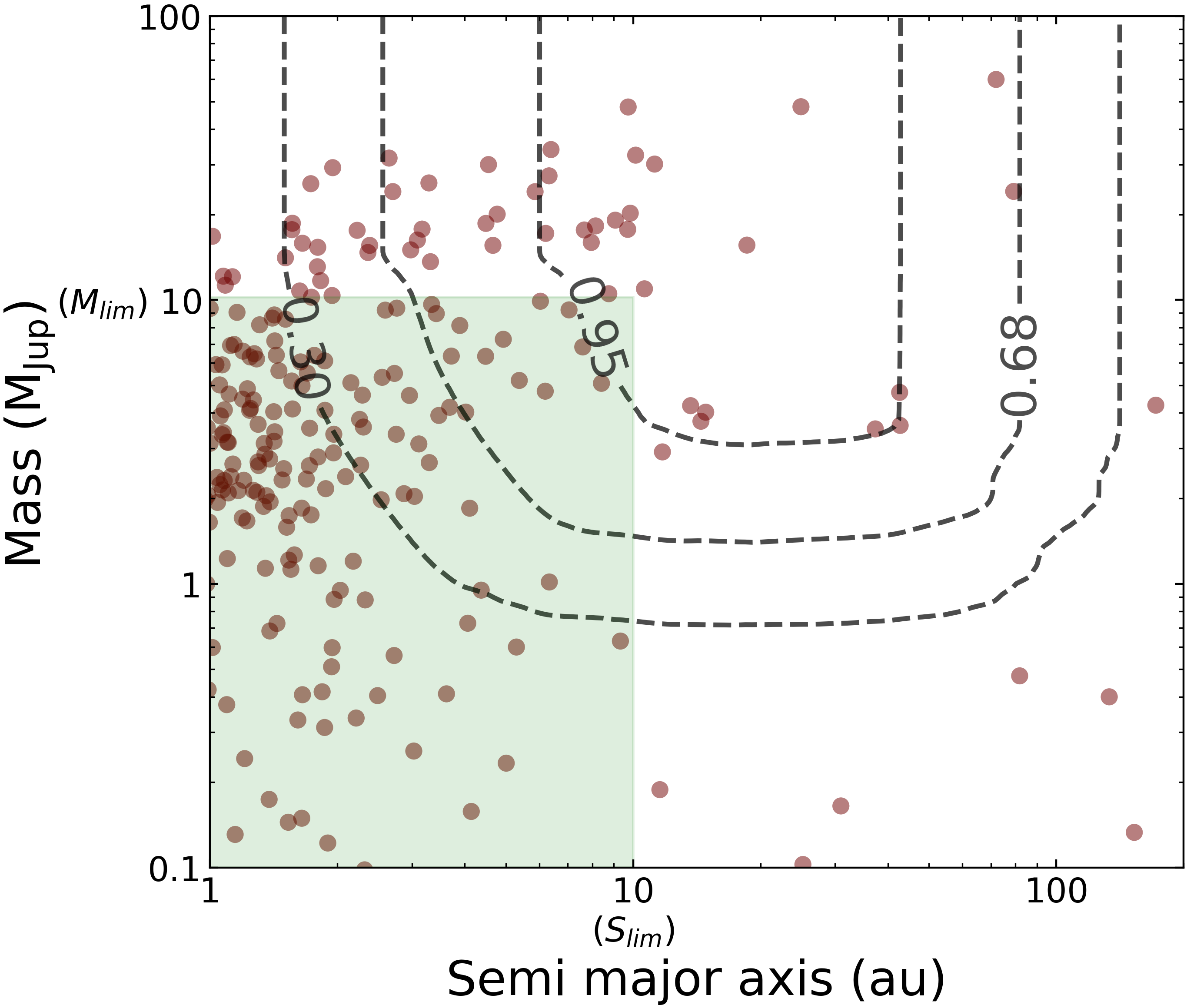
To rank the targets based on their potential to detect planetary mass objects at frost-line type separations, a region in the mass/separation space was first defined. This was defined as the region in detection probability maps where the mass and separation are below the values of and respectively (see Figure 7). Following this, the probability of finding a companion at each grid point was added for all the companions in this parameter space region and all the members of each sample were ranked from the highest probability to the lowest probability. Mathematically, for each member of the sample, the associated rank , is given by,
| (2) |
where is the probability detection value at each grid point and and are the semimajor axis and the mass values respectively. The values of and for this project were selected as and respectively. The semimajor axis upper limit was chosen to ensure sensitivity to frost-line separations (see section 6.2), while the upper limit of was chosen since the hot and cold-start luminosity evolution models can be more easily distinguished for more massive planetary mass companions, (), as discussed for example in Figure 7 of Spiegel & Burrows (2012), see §6.2 for more details. However we do not extend this upper limit beyond , in order to remain in the mass regime consistent with planetary mass companions. As shown in Figure 7, this region is also where there is an increased density in the synthetic planet population from Burn et al. (2021).
The next step was to select a number of candidates from the sample based on this ranking. Once all the stars in each sample were ranked using equation 2 and a list was created, the average detection probability map was calculated. This was done by taking the mean detection probability map of the best candidates, where and is the total number of objects in each sample. Hence, plots were created for each sample ( was the average of the best two stars according to the ranked list (the value), had the average of the best three stars, etc.). After the ranked list was created and average detection probability map of the best stars from each sample was computed, the focus was shifted to calculating the yield (the average number of planets that would be detected with each observation) using the individual stellar masses of the members of the sample.
5 Estimating the planet detection yield
Ranking members in the sample using the method in section 4.3 provides an initial prioritised list of preferred stars to target. However, obtaining a more informative list based on the estimated planet detection yield should take into account any a priori results on the orbital distribution of planets from previous planet detection surveys. To get such a list, we calculate the yield for the stars using the calculated detection probabilities along with the distributions obtained from previous surveys and use this value to rank them. This method also returns the number of companions that would statistically be detected with a given number of observations.
Several works (e.g. Johnson et al., 2007; Bowler et al., 2010; Wagner et al., 2019) provide hints that planet occurrence is likely to be influenced by the host star properties, with the stellar mass likely playing a key role. So, the estimates of the host star masses were refined, as this is expected to be a key variable in the determination of the detection yield, as described below. This is because the yield value is dependant on the stellar mass (see equation 3 in section 5.2).
5.1 Calculating stellar mass estimates
In order to derive individual mass estimates for the sample of host stars, we employed the Manifold Age Determination for Young Stars (madys, Squicciarini et al., 2021; Squicciarini & Bonavita, 2022). Starting from our target list, madys retrieved and cross-matched photometry from Gaia EDR3 (Gaia Collaboration et al., 2021) and 2MASS (Skrutskie et al., 2006), and then applied a correction for interstellar extinction by integrating along the line of sight the 3D extinction map by Leike et al. (2020); the derived values of the extinction in G band () were then used to evaluate the extinction in the chosen photometric band using a total-to-selective absorption ratio and extinction coefficients from Wang & Chen (2019).
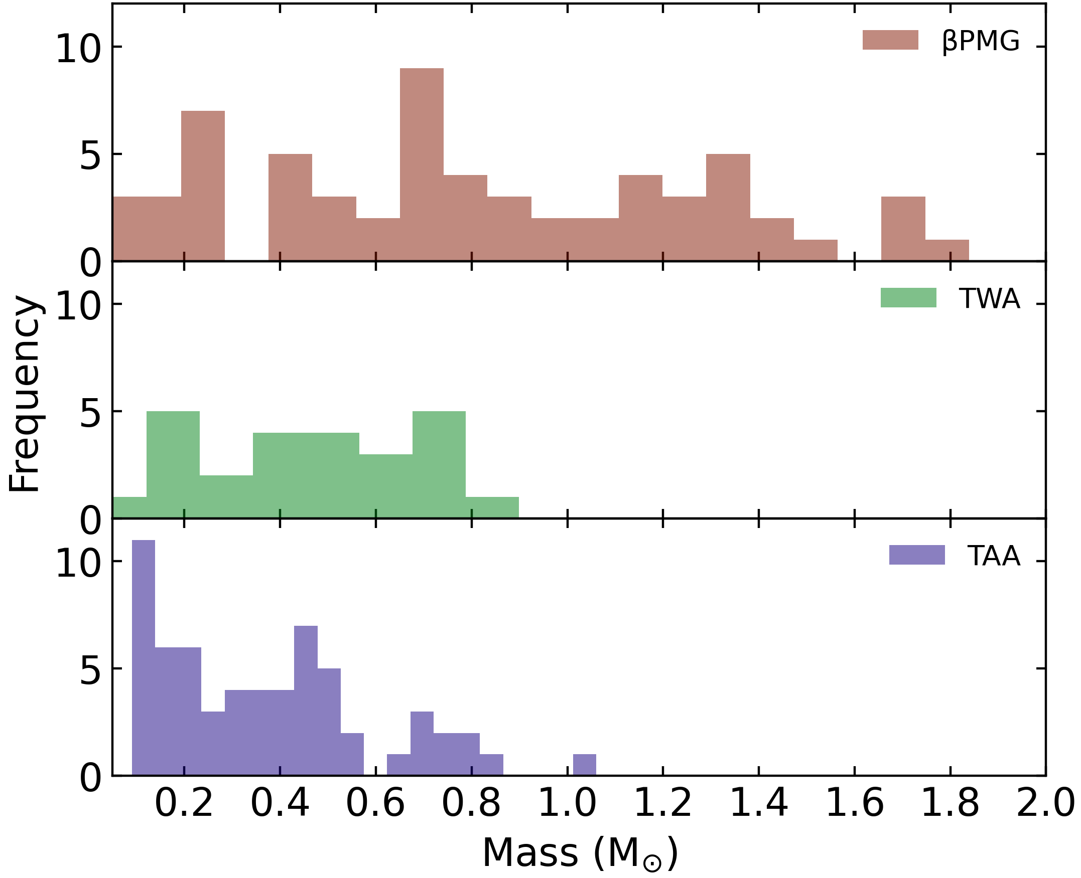
madys then compared, for each star, the derived absolute magnitudes with a grid of theoretical isochrones to simultaneously yield an age and mass estimate. Among several available grids, the PARSEC isochrones (Marigo et al., 2017) were chosen, due to their large dynamical range spanning the entire stellar regime. A constant solar metallicity, appropriate for most nearby star-forming regions, was assumed (D’Orazi et al., 2011). Uncertainties were estimated via a Monte Carlo approach for uncertainty propagation, i.e. by replicating the computation while randomly varying, in a Gaussian fashion, photometric data according to their uncertainties. The resulting mass estimates in the form of histograms for each group are shown in Figure 8. Using these mass values, the yield was calculated for all the members of the sample. This approach is more precise since it uses the photometry for each source. But since all our targets are from well known moving groups/associations (hence the ages are well constrained), we do not expect the values of the masses to have changed significantly from previous work (Carter et al., 2021). So, albeit more accurate, we do not expect the change of approach for the host mass determination to have a significant impact on the final results. The absence of A stars in the TAA sample (as seen in Figure 8) is result of stellar evolution. In the pre-main sequence phase, stars that eventually will be earlier spectral types are still fully convective and descending down the Hayashi track. It is to be noted that there probably are at least some A stars associated with TAA. But without a clear youth indicator such as the presence of a circumstellar disk, distinguishing young early type TAA members from the field can be difficult (Mooley et al., 2013).
5.2 Calculating yield by fine tuning Exo-DMC to stellar masses
The yield is in general evaluated by Exo-DMC as the convolution function , where is the function describing the number of detectable planets, obtained as the sum of the detection probability evaluated by the DMC at each mass/semimajor axis grid point and is the function describing the expected number of planets according to the chosen set of parameter distributions, calculated as:
| (3) |
where is a normalisation constant which makes sure the expected frequency matches the observed one and and are the chosen distributions for semi-major axis and mass, respectively.
For our yield estimate, we chose to adopt two different approaches: one simply extrapolating the latest results from radial velocity (RV hereon) surveys and another from the latest DI results. In both cases the semi-major axis follows a log-normal distribution, while the mass-ratio distribution is a power law for the planetary part and an uniform distribution for the stellar part (see Vigan et al., 2021, for details). Below we describe both distributions in more detail.
-
1.
Extended Radial Velocity
The distribution is taken from Fulton et al. (2021), and is comprised of a broken power-law for the semi-major axis and a mass distribution uniform in logarithmic scale. Although this distribution is drawn from RV data, it has been shown to agree with the DI results (Vigan et al., 2021), so it represent a suitable choice for our analysis. For this case the normalisation factor was calculated to match the results from Vigan et al. (2021), so assuming an overall frequency of 5.6% for companions with masses between 1 and 70 and separations between 5 and 300 au. -
2.
Bimodal Distribution
We also adopt the parametric model outlined in Vigan et al. (2021). The basic assumption of this model is that the observed population is in fact made up of two components representing two different populations of substellar companions: a planet-like population and a binary star-like population. Each component has different parameter distributions and different normalisation factors. Also, this distribution introduces a dependence on the stellar mass, so the planet mass distribution is replaced by a mass ratio () distribution and the other parameters are also dependant on the primary spectral type. So Eq. 3 in this case changes to:(4) where the subscripts PL and BS refer to the planet-like and binary star-like parts of the equation respectively.
The yields hence calculated are reported in Table 1. The values obtained using the extended RV distribution from Fulton et al. (2021) are lower than the ones obtained with the bimodal distribution from Vigan et al. (2021) across all stellar types and groups. The yield values are essentially identical in the filters of F430M and F480M in Table 1. The highest overall yield is produced by TWA at 0.16 planets per star for the Vigan et al. (2021) distribution, but only 0.07 planets per star for the Fulton et al. (2021) distribution. Meanwhile the Pic and TAA groups have yields of planets per star.
| F430M | F480M | ||||||
|---|---|---|---|---|---|---|---|
| Distribution | Spectral Type | Pic | TWA | TAA | Pic | TWA | TAA |
| Vigan et al. (2021) | A | 0.07 | 0.08 | — | 0.07 | 0.08 | — |
| F/G/K | 0.03 | 0.04 | 0.03 | 0.04 | 0.04 | 0.04 | |
| M | 0.16 | 0.17 | 0.06 | 0.16 | 0.18 | 0.06 | |
| Mean | 0.10 | 0.16 | 0.05 | 0.10 | 0.16 | 0.05 | |
| Fulton et al. (2021) | A | 0.04 | 0.03 | — | 0.04 | 0.04 | — |
| F/G/K | 0.05 | 0.06 | 0.04 | 0.05 | 0.06 | 0.04 | |
| M | 0.08 | 0.08 | 0.04 | 0.09 | 0.08 | 0.04 | |
| Mean | 0.07 | 0.07 | 0.04 | 0.07 | 0.08 | 0.04 | |
6 Results and Discussion
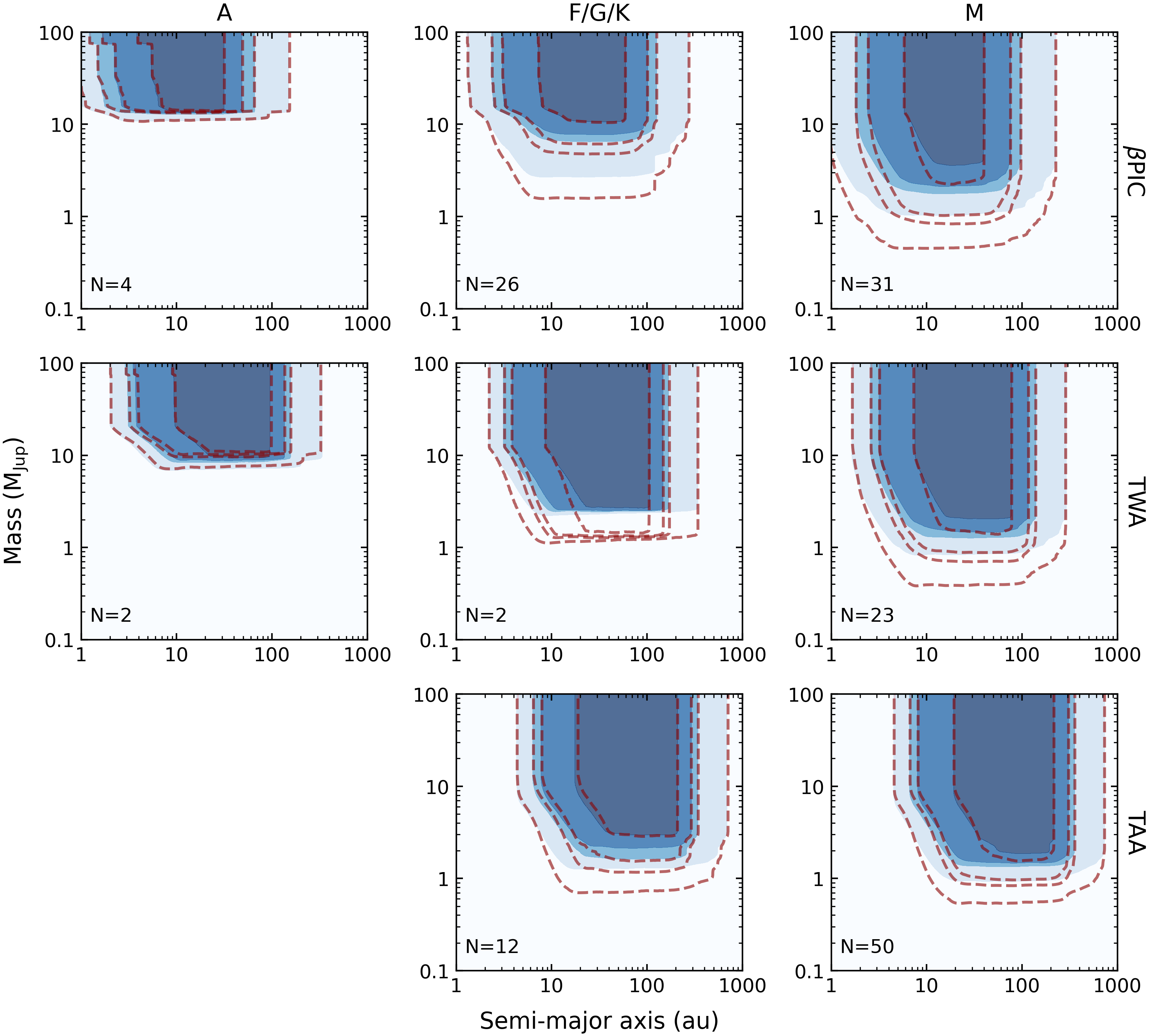
To understand the exquisite mass sensitivity limits attainable using the AMI mode with JWST/NIRISS, we present the detection probability maps of the total sample separated by spectral class (Figure 9), a cumulative average of the stars from each sample with maximum likelihood of a detection, separated by confidence levels (Figure 10) and finally a direct comparison with ground-based instruments (Figure 12).
6.1 Spectral Class
Detection probabilities averaged over each of the spectral classes of the members in the sample provide insight into which type of stars are the most promising for detecting companions in a broader context. Figure 9 separates the members of Pic, TWA and TAA into the spectral groups of A, F/G/K and M stars. The samples of Pic and TWA also have very few earlier type stars causing the probability contours to be slightly discontinuous. In Figure 9 filled contours in the left, middle and right columns, show the average probabilities of the stars in each sample in the spectral groups A, F/G/K and M, in the F430M filter and the dotted lines show the same in the F480M filter. The value of shows the number of stars in each sample in the particular spectral classifications at different probabilities. The contours shown by the four dashed lines and the four subsequently darker regions in each plot are for confidences of 10%, 50%, 68% and 95%. We infer from this result that broadly, the F480M filter clearly outperforms the F430M filter when the aim is to access the lower mass companions. This arises from the fact that substeallar companions with lower masses (and thus cooler temperatures) have a greater fraction of their luminosity at longer wavelengths, making them brighter at (central wavelength of F480M) than at (central wavelength of the F430M filter). There is a clear pattern of increasing depth in each sample towards later spectral types. This is due to the later spectral types being dimmer and hence lower mass companions being potentially more accessible to detect due to a more favourable contrast. The other pattern that emerges from this result is the shift of contour lines outwards (i.e. further away from the host star), with increasing median stellar group distance (see Figure 1), for each spectral type from the samples of Pic to TWA and then TAA.
M stars dominate the stellar mass distribution in all the groups. This makes the average detection probability of the M stars in each group, a reasonable proxy for the group as a whole. For example, in Table 1, for the case of the yield values with the Vigan et al. (2021) distribution in the F480M filter, the mean values of all the stars, and only the M stars, have values 0.16 and 0.18 respectively in the case of TWA. These values are the closest to each other when compared to the mean values of A and F/G/K stars for the same distribution and filter for TWA, which are 0.08 and 0.04 respectively. This trend is seen for all groups, filters and distributions in Table 1. The 10% confidence contour of the detection probabilities in the F480M filter, reaches masses of , in the samples of Pic, TWA and TAA, at separations . Hence, preferentially selecting M stars to observe gives access to lower mass companions, and therefore more effectively taps into the distribution of planets as predicted by Fulton et al. (2021) and Vigan et al. (2021). However, this result is for the average of many targets, and not necessarily an optimised list. In the next section, we show how selecting optimal targets can boost the detection efficiency.
6.2 Best targets to detect close-in companions
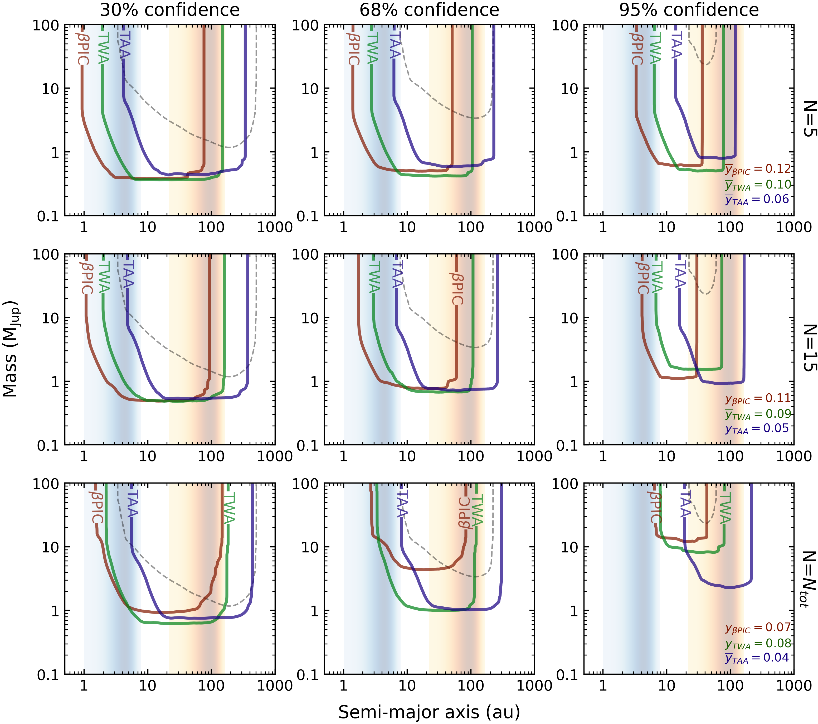
Since the F480M filter provides better performance in terms of reaching lower mass limits, the results presented going forward to determine the best targets to detect close-in companions have been limited to this filter. In Figure 10, we present these results. Ranked by the yield values of each of the members of the samples, obtained using the extended RV distribution (see section 5.2), the first, second and third rows show the averaged detection probabilities for the best 5, 15 and total number of targets respectively (values of in Figure 10), for the members of each sample. The yield from the Extended RV distribution is used rather than the Bimodal distribution to rank the stars since the former dominates the close-in separation parameter space (see Figure 7) which is a better descriptor of the region of parameter space we are concerned with in this work (see section 1), even though the latter produces higher yields. The left, centre and right columns show the 30%, 68% and 95% confidence contours for each sample, including the SHINE survey, shown with a dashed contour. These yield values averaged over stars in Figure 10 are also presented for each sample in the right column.
The H2O and CO frost lines for the stars in our sample were calculated using a methodology from Vigan et al. (2021), which calculates the extent of the frost line using the evaporation temperatures ( and for H2O and CO respectively) from Öberg et al. (2011), a parametric disk temperature profile from Lewis (1974) and observations of protoplanetary disks from Andrews & Williams (2005, 2007a, 2007b). Since frost lines have uncertainties on them, a gradient region demarcated by the smallest and the largest separation values from the range of calculated values for our stars is plotted in Figure 10. The darkest region is the halfway point between the two extremities and the gradient decreases linearly on either side. This is represented in a logarithmic scale in the figure.
For the goal of detecting sub-Jupiter mass companions near the water frost lines at the 68% confidence level, only the most favourable five stars (or 15 stars to some extent) in the Pic and TWA moving groups should be targeted, as evident from Figure 10. In addition to this, the companions with masses greater than near and exterior to these separations can be detected around the best 5 and 15 stars for all the groups (including TAA) with a confidence of 68%. This is particularly remarkable since at higher masses (), the variation of luminosities in the hot and cold start models is more pronounced (Spiegel & Burrows, 2012; Wallace et al., 2021).
The very low infrared background offered by JWST allows impressive sensitivity to low mass companions (e.g. ), even at 95% confidence in some cases (right column in Figure 10), as well as for a majority of the stars in each stellar group (bottom row in Figure 10).
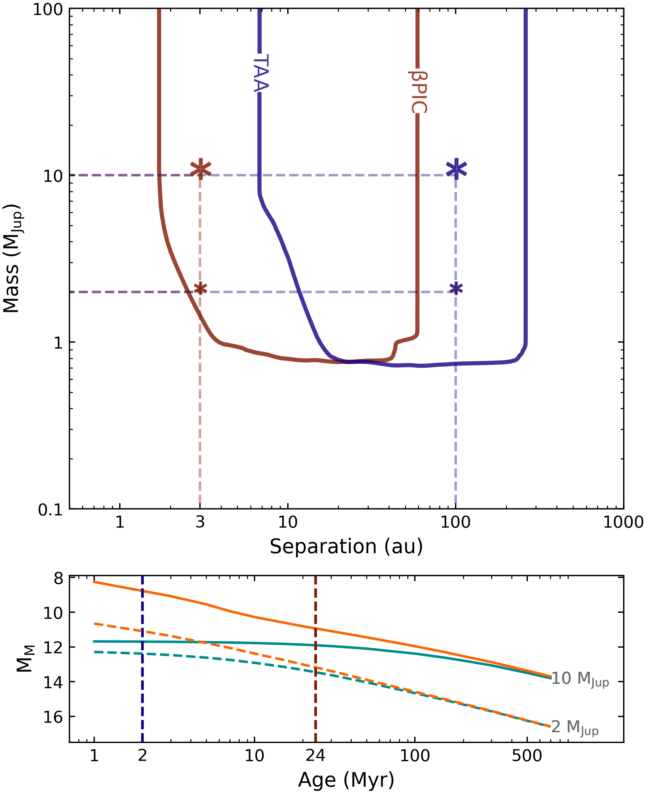
The Gaia mission is expected to unveil thousands of planets (Sozzetti et al., 2014) with reasonably well constrained masses. Most of these will be at separations within , and as we have demonstrated, JWST/AMI can image companions at these locations and measure their mid-infrared luminosities. A tightly constrained dynamical mass, combined with the precise estimate of the bolometric luminosity that can be delivered with JWST/NIRISS/AMI, can then place powerful constraints on the initial energy budget of the companion, and the degree to which it has been modifed due to e.g., energy losses due to accretion shocks at the surface of the planet (e.g., Marley et al., 2007; Marleau & Cumming, 2014). For example, as in Table 1 in Spiegel & Burrows (2012), a old planet of , would have times higher luminosity in the hot start model versus a cold start scenario. A planet at the same age would have a hot-start luminosity times that of a cold-start luminosity. Hence, the population of planets to which AMI is sensitive would be an excellent indicator of initial entropies. As an example, to better understand this approach, the top panel of Figure 11 shows hypothetical detections of and mass planets in Pic and TAA, at and respectively, given the group specific detection probability maps. The bottom panel of Figure 11 shows how given the different ages of Pic and TAA, different luminosities (in M band) would hint at different initial entropies (recreated from Spiegel & Burrows, 2012). As can be seen in the figure, this difference in initial entropy is more pronounced if the companions are younger or if they are more massive.
The cumulative average yield values in Figure 10, decrease as the value of increases since we are averaging over stars which have lower probabilities of hosting companions in the region of the RV distribution. The 95% contour for the case provides the expected shape of the relative detection probabilities for the members of Pic, TWA and TAA because of the subsequent decrease in age (hence the contours go consequently deeper) and the increase in average distance (hence they are restricted to wider orbital separations). This trend is absent in the and cases since the stars hence selected are the ones with the highest yields from their parent samples and have a broad range of distances and masses (see Figures 1 and 8 respectively). This trend also does not manifest in the 68% and the 30% confidence contours since at these confidences, the limiting factor is primarily the sensitivity of the instrument itself, rather than the properties of the stellar groups. Figure 10 also gives a coarse comparison of the performance of the AMI mode with JWST/NIRISS compared to the results from the SHINE survey on the dedicated ground based VLT/SPHERE instrument (Vigan et al., 2021). However, Figure 10 does not present a fully fair comparison since the same set of stars between the two surveys are not being compared. Rather, this exercise compares the best targets from our sample with the entirety of the SHINE survey. So, to give a fairer comparison, we present the results of a direct comparison with the SHINE survey in the following section.
6.3 Direct comparison with the SHINE survey
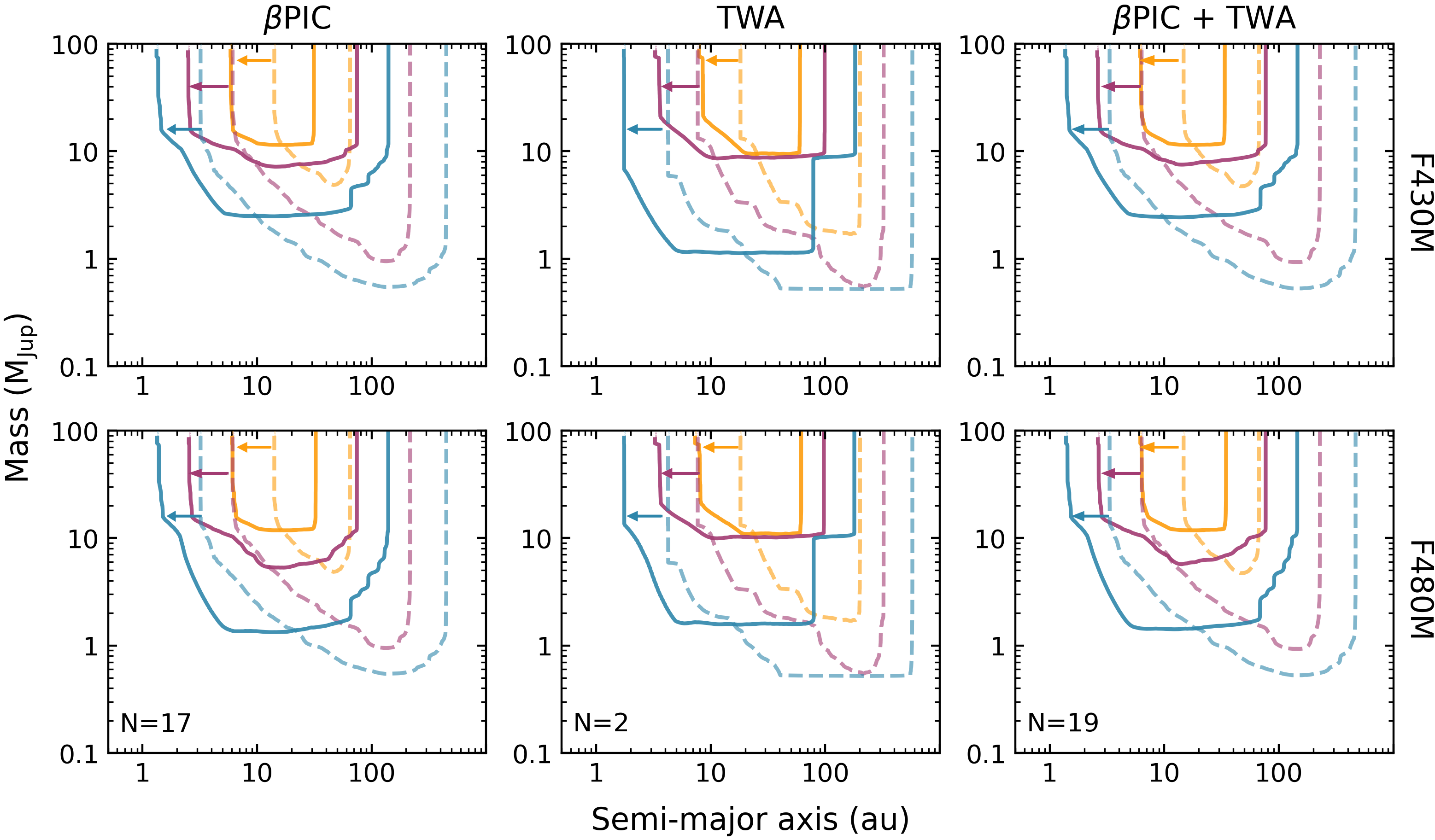
Figure 12 shows the averaged probability maps for those stars in Pic (17 such stars) and TWA (2 such stars) that are common to our sample as well as the SHINE sample. The number of stars considered is given by the value in the plots. None of the stars in TAA were observed with SHINE, most likely since these have declinations too far North to be observed from the southern location of VLT. In the Figure, the 95%, 68% and 30% confidences of the mean detection probabilities are averaged over stars. The solid and the dashed lines represent the JWST/NIRISS and the SHINE survey contours respectively. The first and the second rows show the results from the F430M and F480M filters respectively. The first and the second column show the Pic and TWA stars respectively which are common to both samples.
The right most column shows the average of all 19 cross-matched stars. It is evident from this result that SHINE reaches slightly deeper contrasts when compared to the AMI mode (with the F430M and F480M filters) at larger separations. However, the technical edge achieved by the latter is the accessibility of the regions closer to the host star. In the second row in Figure 12 (F480M filter), the inner limit of the 95% contour for the averaged detection probability for Pic members is brought down from over (with SHINE) to only (with JWST/NIRISS/AMI) for companions with masses . Similar improvements are seen when looking at the TWA averaged members as well as the average of all members from Pic and TWA, across both the filters. This spatial improvement is marked by colour coded arrows in the plots. This makes JWST the ideal observatory to perform a survey for substellar objects near the circumstellar frost lines of nearby stars, since it can achieve a combination of sensitivity at mid-infrared wavelengths and accessibility to close-in separations with better inner working angles in the AMI mode.
Our demonstration that NIRISS operating in AMI mode achieves superior sensitivity at closer orbital separations than SPHERE for the same set of stars is particularly noteworthy given that JWST utilizes a smaller telescope aperture than the one used by VLT ( versus ), as well as operating at a longer wavelength ( for JWST/NIRISS versus 1-2 for VLT/SPHERE), an observational configuration that would indeed return a poorer inner working angle in the case of conventional coronagraphic imaging. This superior performance relative to VLT/SPHERE is due to the interferometric configuration utilized in the AMI mode. In addition to this, observations in the region of the spectrum is extremely important for complementing measurements from observations made by the instruments GPI, VLT/SPHERE and VLTI/GRAVITY at . The long wavelength coverage can provide a much better estimate of the overall bolometric luminosity of the object, which is likely a more secure value from which to draw conclusions about intial entropies. The wavelength range is also particularly well suited to discriminate atmospheric models that incorporate various levels of disequilibrium chemistry that could be due to dynamical processes such as vertical atmospheric mixing (Skemer et al., 2012; Phillips et al., 2020). Differentiating changes in the spectrum that could be induced by such dynamical atmospheric processes from those caused by differences in chemical abundances will ultimately allow tighter constraints to be placed on the intrinsic chemical composition of planetary atmospheres (e.g. Chabrier et al., 2007)
6.4 Kernel phase performance with JWST
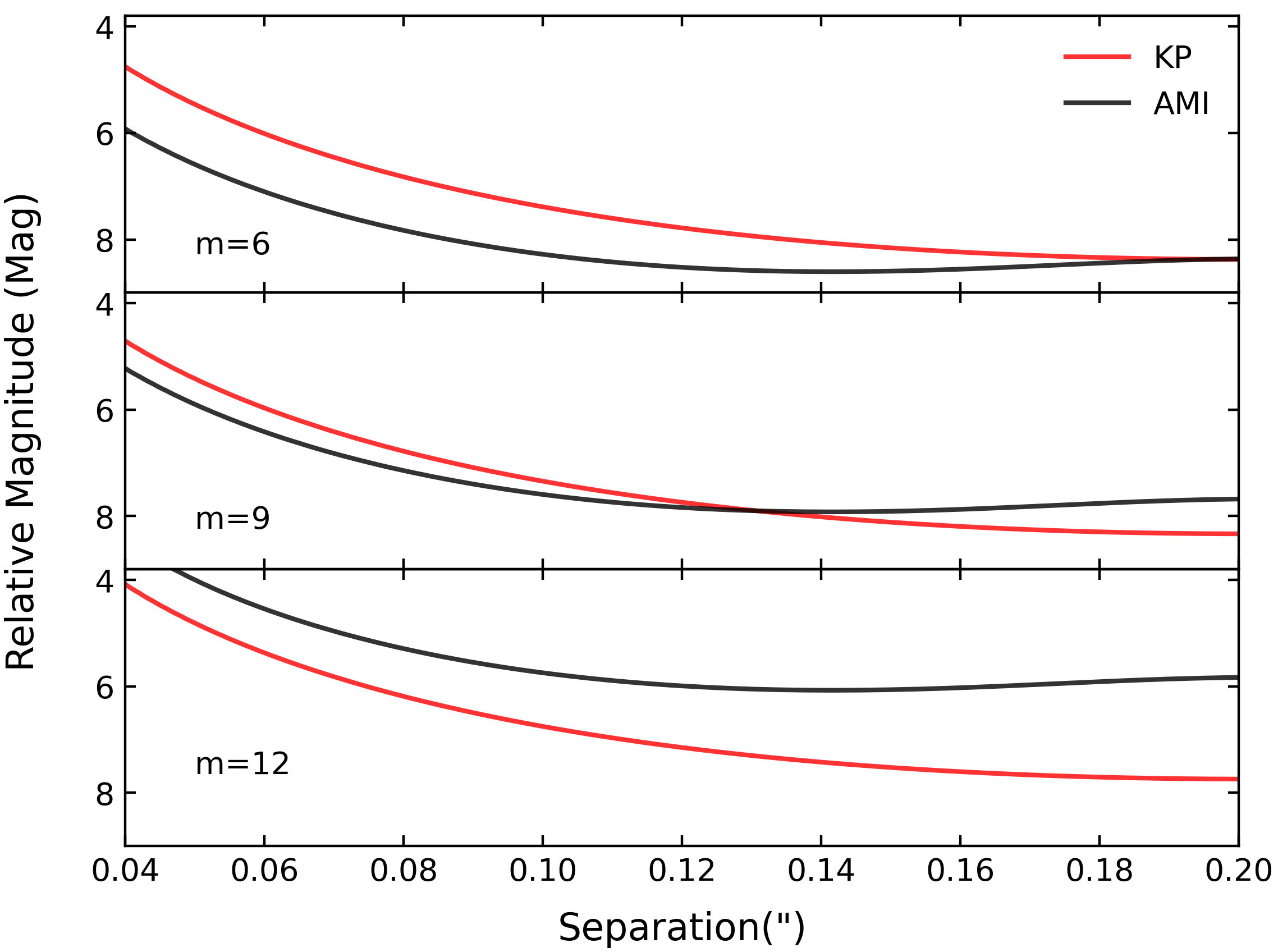
In the high-Strehl regime, the interferometric technique of KP (Martinache, 2010) represents a viable alternative to AMI. Both AMI and KP observations in Sallum & Skemer (2019) were simulated with a fixed exposure time of six hours for each observation (see section 3.1). For fainter targets, AMI requires more integration time compared to KP to reach equivalent contrasts. Hence in this scenario of observing fainter stars, KP outperforms AMI in terms of achieving higher sensitivities for targets with apparent magnitudes . This is shown in Figure 13. For apparent magnitudes of = 6, 9, and 12, the figure shows the contrast curves for simulated observations using KP and AMI with a fixed integration time of six hours. AMI clearly reaches deeper contrasts for brighter targets (, for example in the figure) and KP reaches deeper contrasts for fainter targets (, for example in the figure). However, while planning an actual survey, for bright targets, AMI would not necessarily require six hours for each target and visits can be optimised on a case-by-case basis to achieve similar contrasts and mass ranges presented in sections 3.1 and 6.2 respectively, with lesser exposure times. An actual survey would potentially use both KP and AMI observations for improved efficiency, depending on the brightness of the targets.
6.5 Distinguishing between planetary populations
Using the yield values in Table 1 in conjunction with future survey with JWST/NIRISS/AMI, attempts can be made towards distinguishing planetary populations. For example, if observing 20 stars in the TWA sample results in three companions detections, the bimodal population is more likely to be prevalent in this moving group (, where 0.16 is the mean yield value with the bimodal population described in Vigan et al. 2021). On the contrary if observing 20 stars in the TWA sample results in one companion detection, the underlying population would most likely be better described by the RV population (, where 0.07 is the mean yield value with the Fulton et al. 2021/RV population).
7 Conclusions
We have presented in this work the exquisite capabilities of the AMI mode using JWST/NIRISS to image Jupiter and sub-Jupiter mass exoplanets near the water frost-lines around nearby young stars. Both Pictoris and TW Hydrae moving groups host each to image sub-Jupiter companions with very high confidences (). This is a consequence of the JWST/AMI mode being able to achieve contrasts of at separations of and wider, with sufficient integration times (Soulain et al., 2020). A future survey with this mode to target these detectable planets to put constraints on early entropy conditions of planet formation can be executed in conjunction with a coronagraphy survey of the same stars to save telescope time.
Picking the 10-15 best targets (as shown in Figure 10) either from TWA or Pic, a survey of such stars would take a total of assuming a fixed exposure time of on each target (see §3.1). However, targets which are brighter, would not require as much time to gain the required SNR for a detection and hence this estimated survey time is only an upper limit.
In addition to this, the mode also achieves very high yields for detecting companions in general across the stellar groups, which points to the lucrative nature of a future JWST exoplanet survey with AMI. For example, even the least mean yield values in Table 1 of 0.04-0.05, is greater than most ground based surveys to date, which have values converging at (Bowler & Nielsen, 2018). And the highest mean yield value in Table 1 is 0.16 which is times the minimum value. An optimised survey picking the best candidate stars would have yield values even greater still (see yield values in Tables 3, 4 and 5 in the appendix).
Limiting such a survey to the stars of the Taurus-Auriga association would significantly reduce observatory overheads compared to a survey of Pictoris and TW Hydrae, due to the members of the former being close to each other on the sky plane. Using the stars in a sequence of observations such that they work as as set of mutual reference stars would go a step further in constraining the elapsed time of such a survey. The yield calculations indicate 0.05 detections per star for the association, which is more than the yield of most ground based surveys carried out to date (Nielsen et al., 2019; Vigan et al., 2021). Ground based high contrast imaging platforms with visible-light wave front sensors will not typically be effective for these targets due to their faint optical magnitudes, making JWST the ideal observatory for this task. However, the efficiency of a survey in TAA could be impacted by other variables such as: (1) the presence of protoplanetary discs, which could potentially obscure forming planets; or (2) not carrying out the observations in a non-interruptible sequence which would result in increased telescope overheads. Non-interruptible observations is a mode offered by JWST, which enables the observer to carry out a sequence of observations in a specified time. This will not only save on telescope slew time by optimizing the sequence in order of the closest stars on the sky for the telescope to point, but will also ensure any drift in wave front error, for example due to thermal/structural evolution of the telescope will be minimized.
The upcoming sequential data releases from the Gaia mission are expected to unveil hundreds, if not thousands, of planets orbiting nearby stars in the vicinity of the frost lines of these stars (e.g., Sozzetti et al., 2014). Some fraction of these stars will have ages , and thus will potentially host companions sufficiently self-luminous to be suitable for direct imaging. However, even orbital separations of for a star at correspond to angular separations of , which is comparable to the resolution limit of telescopes operating in the near-infrared. In this paper we have also demonstrated that JWST operating in the AMI mode has comparable sensitivities and inner working angles as VLTI instruments at (Lacour et al., 2019; Nowak et al., 2020; Hinkley et al., 2022a), but crucially provides complementary wavelength coverage at , which is an advantageous wavelength region for discriminating SED shapes that are driven by changes in intrinsic composition, and SED shapes that are being affected by atmospheric processes that lead to disequilibrium chemistry, like vertical atmospheric mixing (Skemer et al., 2012; Konopacky et al., 2013; Phillips et al., 2020; Miles et al., 2020).
Lastly, we await the release of the first science observations from JWST, which would enable us to better understand the contrast limits with the AMI mode, compared to the simulations. This is one of the goals of Director’s Discretionary Early Release Science Program 1386, High Contrast Imaging of Exoplanets and Exoplanetary Systems with JWST (Hinkley et al., 2022b), with which the AMI observation would serve as the benchmark for future observations in this mode and evaluate on-sky contrasts and hence detection probabilities.
Acknowledgements
We thank Adam Kraus for valuable discussion on the stars in the TAA sample. We thank Arthur Vigan for providing us with the methodology to calculate the positions of the frost lines. We thank Ken Rice for useful discussions of planet formation models. We also thank the anonymous referee whose comments have been invaluable towards improving this paper. SR is supported by a Global Excellence Award by the University of Exeter. ALC is supported by a grant from STScI (JWST-ERS-01386) under NASA contract NAS5-03127.
Data Availability
The data underlying this article will be shared on reasonable request to the corresponding author.
References
- Alexander & Armitage (2009) Alexander R. D., Armitage P. J., 2009, ApJ, 704, 989
- Andrews & Williams (2005) Andrews S. M., Williams J. P., 2005, ApJ, 631, 1134
- Andrews & Williams (2007a) Andrews S. M., Williams J. P., 2007a, ApJ, 659, 705
- Andrews & Williams (2007b) Andrews S. M., Williams J. P., 2007b, ApJ, 671, 1800
- Artigau et al. (2014) Artigau É., et al., 2014, in Oschmann Jacobus M. J., Clampin M., Fazio G. G., MacEwen H. A., eds, Society of Photo-Optical Instrumentation Engineers (SPIE) Conference Series Vol. 9143, Space Telescopes and Instrumentation 2014: Optical, Infrared, and Millimeter Wave. p. 914340 (arXiv:1406.6882), doi:10.1117/12.2055191
- Baldwin et al. (1986) Baldwin J. E., Haniff C. A., Mackay C. D., Warner P. J., 1986, Nature, 320, 595
- Baraffe et al. (2003) Baraffe I., Chabrier G., Barman T. S., Allard F., Hauschildt P. H., 2003, A&A, 402, 701
- Baraffe et al. (2015) Baraffe I., Homeier D., Allard F., Chabrier G., 2015, A&A, 577, A42
- Barman et al. (2011) Barman T. S., Macintosh B., Konopacky Q. M., Marois C., 2011, ApJ, 733, 65
- Batalha et al. (2017) Batalha N. E., et al., 2017, PASP, 129, 064501
- Bell et al. (2015) Bell C. P. M., Mamajek E. E., Naylor T., 2015, MNRAS, 454, 593
- Bohn et al. (2020) Bohn A. J., et al., 2020, ApJ, 898, L16
- Boley (2009) Boley A. C., 2009, ApJ, 695, L53
- Bonavita (2020) Bonavita M., 2020, Exo-DMC: Exoplanet Detection Map Calculator (ascl:2010.008)
- Bonavita et al. (2012) Bonavita M., Chauvin G., Desidera S., Gratton R., Janson M., Beuzit J. L., Kasper M., Mordasini C., 2012, A&A, 537, A67
- Bonavita et al. (2013) Bonavita M., de Mooij E. J. W., Jayawardhana R., 2013, PASP, 125, 849
- Bowler (2016) Bowler B. P., 2016, PASP, 128, 102001
- Bowler & Nielsen (2018) Bowler B. P., Nielsen E. L., 2018, Occurrence Rates from Direct Imaging Surveys. p. 155, doi:10.1007/978-3-319-55333-7_155
- Bowler et al. (2010) Bowler B. P., et al., 2010, ApJ, 709, 396
- Burn et al. (2021) Burn R., Schlecker M., Mordasini C., Emsenhuber A., Alibert Y., Henning T., Klahr H., Benz W., 2021, A&A, 656, A72
- Carter et al. (2021) Carter A. L., et al., 2021, MNRAS, 501, 1999
- Chabrier et al. (2007) Chabrier G., Baraffe I., Selsis F., Barman T. S., Hennebelle P., Alibert Y., 2007, Protostars and Planets V, pp 623–638
- Chauvin et al. (2015) Chauvin G., et al., 2015, A&A, 573, A127
- Chauvin et al. (2017) Chauvin G., et al., 2017, A&A, 605, L9
- Cutri et al. (2021) Cutri R. M., et al., 2021, VizieR Online Data Catalog, p. II/328
- D’Orazi et al. (2011) D’Orazi V., Biazzo K., Randich S., 2011, A&A, 526, A103
- Desidera et al. (2021) Desidera S., et al., 2021, A&A, 651, A70
- Doyon et al. (2012) Doyon R., et al., 2012, in Clampin M. C., Fazio G. G., MacEwen H. A., Oschmann Jacobus M. J., eds, Society of Photo-Optical Instrumentation Engineers (SPIE) Conference Series Vol. 8442, Space Telescopes and Instrumentation 2012: Optical, Infrared, and Millimeter Wave. p. 84422R, doi:10.1117/12.926578
- Esposito et al. (2020) Esposito T. M., et al., 2020, AJ, 160, 24
- Fernandes et al. (2019) Fernandes R. B., Mulders G. D., Pascucci I., Mordasini C., Emsenhuber A., 2019, ApJ, 874, 81
- Fortney et al. (2008) Fortney J. J., Lodders K., Marley M. S., Freedman R. S., 2008, ApJ, 678, 1419
- Frelikh et al. (2019) Frelikh R., Jang H., Murray-Clay R. A., Petrovich C., 2019, ApJ, 884, L47
- Fulton et al. (2021) Fulton B. J., et al., 2021, ApJS, 255, 14
- Gagné et al. (2018) Gagné J., et al., 2018, ApJ, 856, 23
- Gaia Collaboration et al. (2016) Gaia Collaboration et al., 2016, A&A, 595, A1
- Gaia Collaboration et al. (2018) Gaia Collaboration et al., 2018, A&A, 616, A1
- Gaia Collaboration et al. (2021) Gaia Collaboration et al., 2021, A&A, 649, A1
- Galicher et al. (2016) Galicher R., et al., 2016, A&A, 594, A63
- Gardner et al. (2006) Gardner J. P., et al., 2006, Space Sci. Rev., 123, 485
- Greenbaum et al. (2015) Greenbaum A. Z., Pueyo L., Sivaramakrishnan A., Lacour S., 2015, ApJ, 798, 68
- Haemmerlé et al. (2019) Haemmerlé L., et al., 2019, A&A, 624, A137
- Haisch et al. (2001) Haisch Karl E. J., Lada E. A., Lada C. J., 2001, ApJ, 553, L153
- Haniff et al. (1987) Haniff C. A., Mackay C. D., Titterington D. J., Sivia D., Baldwin J. E., 1987, Nature, 328, 694
- Hinkley et al. (2011) Hinkley S., Carpenter J. M., Ireland M. J., Kraus A. L., 2011, ApJ, 730, L21+
- Hinkley et al. (2015) Hinkley S., et al., 2015, ApJ, 806, L9
- Hinkley et al. (2021) Hinkley S., et al., 2021, ApJ, 912, 115
- Hinkley et al. (2022a) Hinkley S., et al., 2022a, arXiv e-prints, p. arXiv:2208.04867
- Hinkley et al. (2022b) Hinkley S., et al., 2022b, PASP, 134, 095003
- Hogg et al. (2010) Hogg D. W., Myers A. D., Bovy J., 2010, ApJ, 725, 2166
- JDox Project Team (2016) JDox Project Team 2016, JWST User Documentation (JDox)
- Johnson et al. (2007) Johnson J. A., Butler R. P., Marcy G. W., Fischer D. A., Vogt S. S., Wright J. T., Peek K. M. G., 2007, ApJ, 670, 833
- Kastner et al. (1997) Kastner J. H., Zuckerman B., Weintraub D. A., Forveille T., 1997, Science, 277, 67
- Kenyon & Hartmann (1995) Kenyon S. J., Hartmann L., 1995, ApJS, 101, 117
- Konopacky et al. (2013) Konopacky Q. M., Barman T. S., Macintosh B. A., Marois C., 2013, Science, 339, 1398
- Kratter et al. (2010) Kratter K. M., Murray-Clay R. A., Youdin A. N., 2010, ApJ, 710, 1375
- Kraus et al. (2017) Kraus A. L., Herczeg G. J., Rizzuto A. C., Mann A. W., Slesnick C. L., Carpenter J. M., Hillenbrand L. A., Mamajek E. E., 2017, ApJ, 838, 150
- Lacour et al. (2019) Lacour S., et al., 2019, A&A, 624, A99
- Lagrange et al. (2009) Lagrange A. M., et al., 2009, A&A, 493, L21
- Langlois et al. (2021) Langlois M., et al., 2021, A&A, 651, A71
- Leike et al. (2020) Leike R. H., Glatzle M., Enßlin T. A., 2020, A&A, 639, A138
- Lewis (1974) Lewis J. S., 1974, Science, 186, 440
- Lloyd et al. (2006) Lloyd J. P., Martinache F., Ireland M. J., Monnier J. D., Pravdo S. H., Shaklan S. B., Tuthill P. G., 2006, ApJ, 650, L131
- Malo et al. (2014) Malo L., Doyon R., Feiden G. A., Albert L., Lafrenière D., Artigau É., Gagné J., Riedel A., 2014, ApJ, 792, 37
- Marigo et al. (2017) Marigo P., et al., 2017, ApJ, 835, 77
- Marleau & Cumming (2014) Marleau G. D., Cumming A., 2014, MNRAS, 437, 1378
- Marley et al. (2007) Marley M. S., Fortney J. J., Hubickyj O., Bodenheimer P., Lissauer J. J., 2007, ApJ, 655, 541
- Marois et al. (2008) Marois C., Macintosh B., Barman T., Zuckerman B., Song I., Patience J., Lafrenière D., Doyon R., 2008, Science, 322, 1348
- Martinache (2010) Martinache F., 2010, ApJ, 724, 464
- Matthews et al. (2017) Matthews E., et al., 2017, ApJ, 843, L12
- Miles et al. (2020) Miles B. E., et al., 2020, AJ, 160, 63
- Milli et al. (2017) Milli J., et al., 2017, A&A, 599, A108
- Mollière et al. (2022) Mollière P., et al., 2022, ApJ, 934, 74
- Monnier et al. (2007) Monnier J. D., Tuthill P. G., Danchi W. C., Murphy N., Harries T. J., 2007, ApJ, 655, 1033
- Mooley et al. (2013) Mooley K., Hillenbrand L., Rebull L., Padgett D., Knapp G., 2013, ApJ, 771, 110
- Mordasini et al. (2016) Mordasini C., van Boekel R., Mollière P., Henning T., Benneke B., 2016, ApJ, 832, 41
- Mordasini et al. (2017) Mordasini C., Marleau G. D., Mollière P., 2017, A&A, 608, A72
- Nielsen et al. (2019) Nielsen E. L., et al., 2019, AJ, 158, 13
- Nowak et al. (2020) Nowak M., et al., 2020, A&A, 642, L2
- Öberg et al. (2011) Öberg K. I., Murray-Clay R., Bergin E. A., 2011, ApJ, 743, L16
- Perrin et al. (2014) Perrin M. D., Sivaramakrishnan A., Lajoie C.-P., Elliott E., Pueyo L., Ravindranath S., Albert L., 2014, in Oschmann Jacobus M. J., Clampin M., Fazio G. G., MacEwen H. A., eds, Society of Photo-Optical Instrumentation Engineers (SPIE) Conference Series Vol. 9143, Space Telescopes and Instrumentation 2014: Optical, Infrared, and Millimeter Wave. p. 91433X, doi:10.1117/12.2056689
- Phillips et al. (2020) Phillips M. W., et al., 2020, A&A, 637, A38
- Poleski et al. (2021) Poleski R., et al., 2021, Acta Astron., 71, 1
- Pollack et al. (1996) Pollack J. B., Hubickyj O., Bodenheimer P., Lissauer J. J., Podolak M., Greenzweig Y., 1996, Icarus, 124, 62
- Pontoppidan et al. (2016) Pontoppidan K. M., et al., 2016, in Peck A. B., Seaman R. L., Benn C. R., eds, Society of Photo-Optical Instrumentation Engineers (SPIE) Conference Series Vol. 9910, Observatory Operations: Strategies, Processes, and Systems VI. p. 991016 (arXiv:1707.02202), doi:10.1117/12.2231768
- Readhead et al. (1988) Readhead A. C. S., Nakajima T. S., Pearson T. J., Neugebauer G., Oke J. B., Sargent W. L. W., 1988, AJ, 95, 1278
- Rieke et al. (2005) Rieke M. J., Kelly D., Horner S., 2005, in Heaney J. B., Burriesci L. G., eds, Society of Photo-Optical Instrumentation Engineers (SPIE) Conference Series Vol. 5904, Cryogenic Optical Systems and Instruments XI. pp 1–8, doi:10.1117/12.615554
- STScI Development Team (2013) STScI Development Team 2013, pysynphot: Synthetic photometry software package (ascl:1303.023)
- Sallum & Skemer (2019) Sallum S., Skemer A., 2019. p. 018001 (arXiv:1901.01266), doi:10.1117/1.JATIS.5.1.018001
- Sivaramakrishnan et al. (2009) Sivaramakrishnan A., et al., 2009, in Shaklan S. B., ed., Society of Photo-Optical Instrumentation Engineers (SPIE) Conference Series Vol. 7440, Techniques and Instrumentation for Detection of Exoplanets IV. p. 74400Y, doi:10.1117/12.826633
- Sivaramakrishnan et al. (2012) Sivaramakrishnan A., et al., 2012, in Clampin M. C., Fazio G. G., MacEwen H. A., Oschmann Jacobus M. J., eds, Society of Photo-Optical Instrumentation Engineers (SPIE) Conference Series Vol. 8442, Space Telescopes and Instrumentation 2012: Optical, Infrared, and Millimeter Wave. p. 84422S, doi:10.1117/12.925565
- Skemer et al. (2012) Skemer A. J., et al., 2012, ApJ, 753, 14
- Skrutskie et al. (2006) Skrutskie M. F., et al., 2006, AJ, 131, 1163
- Soulain et al. (2020) Soulain A., et al., 2020, in Society of Photo-Optical Instrumentation Engineers (SPIE) Conference Series. p. 1144611 (arXiv:2201.01524), doi:10.1117/12.2560804
- Sozzetti et al. (2014) Sozzetti A., Giacobbe P., Lattanzi M. G., Micela G., Morbidelli R., Tinetti G., 2014, MNRAS, 437, 497
- Spiegel & Burrows (2012) Spiegel D. S., Burrows A., 2012, ApJ, 745, 174
- Squicciarini & Bonavita (2022) Squicciarini V., Bonavita M., 2022, A&A, 666, A15
- Squicciarini et al. (2021) Squicciarini V., Gratton R., Bonavita M., Mesa D., 2021, MNRAS, 507, 1381
- Tuthill et al. (2000) Tuthill P. G., Monnier J. D., Danchi W. C., Wishnow E. H., Haniff C. A., 2000, PASP, 112, 555
- Upton & Ellerbroek (2004) Upton R., Ellerbroek B., 2004, Optics Letters, 29, 2840
- Vigan et al. (2017) Vigan A., et al., 2017, A&A, 603, A3
- Vigan et al. (2021) Vigan A., et al., 2021, A&A, 651, A72
- Wagner et al. (2019) Wagner K., Apai D., Kratter K. M., 2019, ApJ, 877, 46
- Wallace et al. (2021) Wallace A. L., Ireland M. J., Federrath C., 2021, MNRAS, 508, 2515
- Wang & Chen (2019) Wang S., Chen X., 2019, ApJ, 877, 116
- Woodruff et al. (2008) Woodruff H. C., Tuthill P. G., Monnier J. D., Ireland M. J., Bedding T. R., Lacour S., Danchi W. C., Scholz M., 2008, ApJ, 673, 418
- Wright et al. (2010) Wright E. L., et al., 2010, AJ, 140, 1868
- Zuckerman et al. (2001) Zuckerman B., Song I., Bessell M. S., Webb R. A., 2001, ApJ, 562, L87
Appendix A Contrast curve simulation variables
| F430M | F480M | |||||||||
|---|---|---|---|---|---|---|---|---|---|---|
| Ms | eff | eff | ||||||||
| 5.7 | 35 | 2070 | 31 | 5246 | 0.97 | 39 | 1858 | 19 | 5261 | 0.97 |
| 5.8 | 38 | 1907 | 15 | 5258 | 0.97 | 42 | 1725 | 31 | 5271 | 0.98 |
| 5.9 | 42 | 1725 | 31 | 5271 | 0.98 | 46 | 1575 | 31 | 5282 | 0.98 |
| 6.0 | 46 | 1575 | 31 | 5282 | 0.98 | 51 | 1421 | 10 | 5294 | 0.98 |
| 6.1 | 50 | 1449 | 31 | 5292 | 0.98 | 56 | 1294 | 17 | 5303 | 0.98 |
| 6.2 | 55 | 1317 | 46 | 5302 | 0.98 | 61 | 1188 | 13 | 5311 | 0.98 |
| 6.3 | 61 | 1188 | 13 | 5311 | 0.98 | 67 | 1081 | 54 | 5319 | 0.99 |
| 6.4 | 67 | 1081 | 54 | 5319 | 0.99 | 74 | 979 | 35 | 5327 | 0.99 |
| 6.5 | 73 | 992 | 65 | 5326 | 0.99 | 81 | 894 | 67 | 5333 | 0.99 |
| 6.6 | 80 | 906 | — | 5332 | 0.99 | 89 | 814 | 35 | 5339 | 0.99 |
| 6.7 | 88 | 823 | 57 | 5339 | 0.99 | 98 | 739 | 59 | 5345 | 0.99 |
| 6.8 | 96 | 755 | — | 5344 | 0.99 | 107 | 677 | 42 | 5349 | 0.99 |
| 6.9 | 106 | 683 | 83 | 5349 | 0.99 | 117 | 619 | 58 | 5354 | 0.99 |
| 7.0 | 116 | 624 | 97 | 5353 | 0.99 | 129 | 561 | 112 | 5358 | 0.99 |
| 7.1 | 127 | 570 | 91 | 5357 | 0.99 | 141 | 514 | 7 | 5362 | 0.99 |
| 7.2 | 140 | 517 | 101 | 5361 | 0.99 | 155 | 467 | 96 | 5365 | 0.99 |
| 7.3 | 153 | 473 | 112 | 5365 | 0.99 | 170 | 426 | 61 | 5368 | 0.99 |
| 7.4 | 168 | 431 | 73 | 5368 | 0.99 | 186 | 389 | 127 | 5371 | 0.99 |
| 7.5 | 184 | 393 | 169 | 5371 | 0.99 | 205 | 353 | 116 | 5374 | 1.00 |
| 7.6 | 202 | 358 | 165 | 5373 | 1.00 | 224 | 323 | 129 | 5376 | 1.00 |
| 7.7 | 221 | 327 | 214 | 5375 | 1.00 | 246 | 294 | 157 | 5378 | 1.00 |
| 7.8 | 243 | 298 | 67 | 5378 | 1.00 | 270 | 268 | 121 | 5380 | 1.00 |
| 7.9 | 266 | 272 | 129 | 5380 | 1.00 | 296 | 244 | 257 | 5382 | 1.00 |
| 8.0 | 292 | 248 | 65 | 5381 | 1.00 | 324 | 223 | 229 | 5383 | 1.00 |
| 8.1 | 320 | 226 | 161 | 5383 | 1.00 | 356 | 203 | 213 | 5385 | 1.00 |
| 8.2 | 351 | 206 | 175 | 5384 | 1.00 | 390 | 185 | 331 | 5386 | 1.00 |
| 8.3 | 385 | 188 | 101 | 5386 | 1.00 | 428 | 169 | 149 | 5387 | 1.00 |
| 8.4 | 422 | 171 | 319 | 5387 | 1.00 | 469 | 154 | 255 | 5388 | 1.00 |
| 8.5 | 463 | 156 | 253 | 5388 | 1.00 | 514 | 141 | 7 | 5389 | 1.00 |
| 8.6 | 508 | 142 | 345 | 5389 | 1.00 | 564 | 128 | 289 | 5390 | 1.00 |
| 8.7 | 557 | 130 | 71 | 5390 | 1.00 | 618 | 117 | 175 | 5391 | 1.00 |
| 8.8 | 611 | 118 | 383 | 5391 | 1.00 | 678 | 106 | 613 | 5392 | 1.00 |
| 8.9 | 670 | 108 | 121 | 5392 | 1.00 | 743 | 97 | 410 | 5393 | 1.00 |
| 9.0 | 735 | 98 | 451 | 5393 | 1.00 | 800 | 90 | 481 | 5393 | 1.00 |
| 9.1-12.7 | 799 | 90 | 571 | 5393 | 1.00 | 800 | 90 | 481 | 5393 | 1.00 |
Appendix B List of stars in the sample
| Rank | Gaia DR2 ID | Distance (pc) | Spectral Type | ||||
|---|---|---|---|---|---|---|---|
| 1 | 3230008650057256960 | 21.00 | M9 | 11.93 | 12.16 | 0.147 | 0.147 |
| 2 | 5355751581627180288 | 19.79 | M5 | 8.64 | 8.82 | 0.129 | 0.138 |
| 3 | 3238965099979863296 | 27.63 | M4 | 9.08 | 9.24 | 0.115 | 0.130 |
| 4 | 6603693881832177792 | 20.87 | M4 | 7.87 | 8.03 | 0.115 | 0.127 |
| 5 | 2901786974419551488 | 29.76 | M4 | 9.27 | 9.43 | 0.113 | 0.124 |
| 6 | 6794047652729201024 | 9.71 | M1 | 5.23 | 5.37 | 0.112 | 0.122 |
| 7 | 2324205785406060928 | 37.38 | M6 | 11.65 | 11.84 | 0.109 | 0.120 |
| 8 | 3216753556349327232 | 38.52 | M5 | 10.67 | 10.84 | 0.102 | 0.118 |
| 9 | 3291643148740384128 | 23.79 | M2 | 7.26 | 7.42 | 0.100 | 0.116 |
| 10 | 3216729878197029120 | 38.02 | M5 | 9.51 | 9.68 | 0.100 | 0.114 |
| 11 | 2727844441062478464 | 37.39 | M5 | 10.01 | 10.18 | 0.100 | 0.113 |
| 12 | 2315841869173294080 | 35.03 | M3 | 8.97 | 9.12 | 0.098 | 0.112 |
| 13 | 2433191886212246784 | 27.45 | M0 | 7.57 | 7.71 | 0.098 | 0.111 |
| 14 | 3231945508509506176 | 24.40 | M0 | 7.23 | 7.36 | 0.097 | 0.110 |
| 15 | 2477870708709917568 | 37.28 | M4 | 9.12 | 9.28 | 0.097 | 0.109 |
| 16 | 6833291426043854976 | 33.60 | M5 | 8.50 | 8.66 | 0.096 | 0.108 |
| 17 | 6577998398172195840 | 48.72 | M5 | 11.75 | 11.94 | 0.096 | 0.107 |
| 18 | 4707563810327288192 | 36.82 | M3 | 8.77 | 8.92 | 0.095 | 0.107 |
| 19 | 4764027962957023104 | 26.87 | M0 | 7.22 | 7.35 | 0.094 | 0.106 |
| 20 | 2899492637251200512 | 33.77 | M3 | 8.14 | 8.30 | 0.093 | 0.105 |
| 21 | 6800238044930953600 | 43.66 | M4 | 9.80 | 9.97 | 0.093 | 0.105 |
| 22 | 68012529415816832 | 50.70 | M8 | 12.28 | 12.56 | 0.091 | 0.104 |
| 23 | 3216729573251961856 | 36.74 | M1 | 8.02 | 8.16 | 0.089 | 0.104 |
| 24 | 6806301370519190912 | 43.88 | M4 | 8.76 | 8.92 | 0.085 | 0.103 |
| 25 | 6649786646225001984 | 51.65 | M4 | 10.59 | 10.72 | 0.083 | 0.102 |
| 26 | 6382640367603744128 | 36.72 | K7 | 7.91 | 8.04 | 0.083 | 0.101 |
| 27 | 132362959259196032 | 40.94 | K7 | 8.12 | 8.23 | 0.081 | 0.101 |
| 28 | 5266270443442455040 | 39.11 | K4 | 7.72 | 7.82 | 0.077 | 0.100 |
| 29 | 5935776714456619008 | 50.79 | M3 | 8.69 | 8.82 | 0.071 | 0.099 |
| 30 | 6736232346363422336 | 49.46 | K8 | 8.55 | 8.68 | 0.070 | 0.098 |
| 31 | 6747467224874108288 | 51.31 | K9 | 8.91 | 9.04 | 0.068 | 0.097 |
| 32 | 3393207610483520896 | 53.09 | K2 | 8.69 | 8.81 | 0.067 | 0.096 |
| 33 | 87555176071871744 | 70.75 | M6 | 12.56 | 12.75 | 0.066 | 0.095 |
| 34 | 4067828843907821824 | 63.81 | M2 | 9.52 | 9.67 | 0.065 | 0.094 |
| 35 | 2622845684814477696 | 25.52 | F8 | 5.21 | 5.25 | 0.065 | 0.093 |
| 36 | 3009908378049913216 | 26.84 | F8 | 5.45 | 5.49 | 0.065 | 0.092 |
| 37 | 5882581895219921024 | 38.72 | K0 | 6.29 | 6.36 | 0.059 | 0.092 |
| 38 | 94988050769772288 | 52.77 | K0 | 7.62 | 7.73 | 0.058 | 0.091 |
| 39 | 5811866422581688320 | 30.35 | K1 | 5.27 | 5.34 | 0.058 | 0.090 |
| 40 | 6655168686921108864 | 47.25 | G9 | 7.08 | 7.14 | 0.058 | 0.089 |
| 41 | 5945104588806333824 | 76.64 | M2 | 10.29 | 10.44 | 0.057 | 0.088 |
| 42 | 6663346029775435264 | 71.27 | M0 | 9.31 | 9.44 | 0.054 | 0.087 |
| 43 | 6643589352010758400 | 47.78 | F6 | 6.40 | 6.42 | 0.052 | 0.087 |
| 44 | 5924485966955008896 | 67.61 | K1 | 8.25 | 8.32 | 0.051 | 0.086 |
| 45 | 6847146784384459648 | 50.11 | F5 | 6.44 | 6.47 | 0.051 | 0.085 |
| 46 | 6882840883190250752 | 45.91 | F8 | 6.31 | 6.34 | 0.050 | 0.084 |
| 47 | 3205095125321700480 | 29.91 | F0 | 4.83 | 4.85 | 0.049 | 0.084 |
| 48 | 6760846563417053056 | 74.34 | M0 | 8.99 | 9.12 | 0.049 | 0.083 |
| 49 | 4792774797545105664 | 19.63 | A6 | 3.70 | 3.72 | 0.049 | 0.082 |
| 50 | 4045698423617983488 | 71.48 | K5 | 8.17 | 8.28 | 0.047 | 0.081 |
| 51 | 6631762764424312960 | 50.57 | F5 | 6.62 | 6.65 | 0.046 | 0.081 |
| 52 | 6438274350302427776 | 28.79 | A7 | 4.58 | 4.61 | 0.046 | 0.080 |
| 53 | 107774202769886848 | 39.56 | F5 | 5.50 | 5.53 | 0.046 | 0.079 |
| 54 | 5946515438335508864 | 65.80 | F8 | 7.63 | 7.67 | 0.045 | 0.079 |
| 55 | 6470519830886970880 | 63.67 | F5 | 7.06 | 7.09 | 0.045 | 0.078 |
| 56 | 6702775135228913280 | 49.30 | F6 | 6.24 | 6.27 | 0.044 | 0.078 |
| 57 | 5849837854817580672 | 16.40 | A7 | 2.47 | 2.50 | 0.042 | 0.077 |
| 58 | 4051081838710783232 | 80.48 | G5 | 7.76 | 7.82 | 0.036 | 0.076 |
| 59 | 6724105656508792576 | 43.97 | A6 | 4.65 | 4.68 | 0.035 | 0.075 |
| 60 | 4038504701367019648 | 82.71 | G0 | 7.77 | 7.82 | 0.034 | 0.075 |
| 61 | 4057573802035360896 | 83.29 | F3 | 7.29 | 7.31 | 0.030 | 0.074 |
| Rank | Gaia DR2 ID | Distance (pc) | Spectral Type | ||||
|---|---|---|---|---|---|---|---|
| 1 | 3478519134297202560 | 46.71 | M8 | 12.24 | 12.50 | 0.106 | 0.106 |
| 2 | 3536988276442796800 | 43.80 | M6 | 10.34 | 10.52 | 0.104 | 0.105 |
| 3 | 3478940625208241920 | 48.90 | M5 | 9.81 | 9.99 | 0.101 | 0.104 |
| 4 | 3481965141177021568 | 47.42 | M5 | 9.80 | 9.97 | 0.098 | 0.102 |
| 5 | 6146137782994601984 | 52.93 | M3 | 10.19 | 10.34 | 0.093 | 0.100 |
| 6 | 5396978667759696000 | 37.05 | M4 | 7.52 | 7.69 | 0.093 | 0.099 |
| 7 | 3485098646237003392 | 45.96 | M3 | 8.51 | 8.66 | 0.088 | 0.097 |
| 8 | 5460240959047928832 | 52.54 | M3 | 8.83 | 9.00 | 0.086 | 0.096 |
| 9 | 5444751795151480320 | 34.10 | M2 | 7.93 | 10.52 | 0.084 | 0.095 |
| 10 | 6150861598480158336 | 53.60 | M0 | 8.94 | 8.55 | 0.083 | 0.093 |
| 11 | 5467714064704570112 | 61.17 | M5 | 10.22 | 10.36 | 0.082 | 0.092 |
| 12 | 6146107993101452160 | 57.48 | M2 | 9.27 | 9.42 | 0.082 | 0.092 |
| 13 | 5452498537466667776 | 45.94 | M2 | 7.74 | 7.88 | 0.081 | 0.091 |
| 14 | 3465989374664029184 | 62.58 | M4 | 10.81 | 10.98 | 0.079 | 0.090 |
| 15 | 3468438639892079360 | 64.35 | M5 | 10.58 | 10.76 | 0.078 | 0.089 |
| 16 | 6147044433411060224 | 63.60 | M2 | 9.57 | 9.73 | 0.076 | 0.088 |
| 17 | 5398663566249861120 | 49.67 | M2 | 7.72 | 7.87 | 0.075 | 0.087 |
| 18 | 3466308095597260032 | 56.82 | M2 | 8.79 | 8.94 | 0.074 | 0.087 |
| 19 | 5399220743767211776 | 59.85 | M1 | 8.71 | 8.84 | 0.071 | 0.086 |
| 20 | 5396105586807802880 | 65.40 | M1 | 9.20 | 9.35 | 0.071 | 0.085 |
| 21 | 5378040370245563008 | 72.25 | M0 | 10.06 | 10.22 | 0.069 | 0.084 |
| 22 | 5401795662560500352 | 60.14 | K6 | 8.00 | 8.12 | 0.068 | 0.084 |
| 23 | 3465944500845668224 | 70.76 | M4 | 9.67 | 9.84 | 0.068 | 0.083 |
| 24 | 6132146982868270976 | 80.21 | M3 | 9.49 | 9.65 | 0.060 | 0.082 |
| 25 | 3463395519357786752 | 76.49 | K5 | 8.78 | 8.90 | 0.057 | 0.081 |
| 26 | 3532027383058513664 | 54.60 | A1 | 5.56 | 5.59 | 0.043 | 0.080 |
| 27 | 6147117727029871360 | 70.77 | A0 | 5.92 | 5.94 | 0.032 | 0.078 |
| Rank | Gaia DR2 ID | Distance (pc) | Spectral Type | ||||
|---|---|---|---|---|---|---|---|
| 1 | 3401526068784149504 | 58.34 | M0 | 9.47 | 9.64 | 0.101 | 0.101 |
| 2 | 3403016495451584000 | 102.08 | K4 | 9.51 | 9.65 | 0.055 | 0.078 |
| 3 | 146764465639042176 | 125.48 | M7 | 11.96 | 12.13 | 0.048 | 0.068 |
| 4 | 146277553787186048 | 126.77 | M7 | 12.16 | 12.34 | 0.046 | 0.062 |
| 5 | 3416236744087968768 | 118.44 | K7 | 9.77 | 9.92 | 0.046 | 0.059 |
| 6 | 151028990206478080 | 126.97 | M6 | 11.50 | 11.67 | 0.046 | 0.057 |
| 7 | 147799209159857280 | 126.51 | M6 | 11.10 | 11.27 | 0.046 | 0.055 |
| 8 | 164409359522965120 | 128.03 | M5 | 11.90 | 12.08 | 0.045 | 0.054 |
| 9 | 150908490604475520 | 132.86 | M5 | 12.00 | 12.18 | 0.045 | 0.053 |
| 10 | 146487560507840768 | 123.63 | M4 | 10.76 | 10.93 | 0.045 | 0.052 |
| 11 | 164550882989640192 | 117.39 | M2 | 9.43 | 9.58 | 0.045 | 0.052 |
| 12 | 164513022853468160 | 124.69 | M6 | 11.22 | 11.39 | 0.043 | 0.051 |
| 13 | 163177116226018944 | 129.18 | M5 | 10.89 | 11.07 | 0.043 | 0.050 |
| 14 | 147523605402800256 | 119.46 | M2 | 9.71 | 9.86 | 0.043 | 0.050 |
| 15 | 162535345034688768 | 129.35 | M2 | 10.53 | 10.68 | 0.043 | 0.049 |
| 16 | 164470794735041152 | 135.11 | M6 | 12.12 | 12.30 | 0.042 | 0.049 |
| 17 | 151793082068521856 | 127.01 | K8 | 9.88 | 10.01 | 0.042 | 0.048 |
| 18 | 151373820245230080 | 129.60 | M4 | 9.81 | 9.98 | 0.041 | 0.048 |
| 19 | 164705368668853120 | 132.21 | M2 | 10.09 | 10.24 | 0.041 | 0.048 |
| 20 | 148037764527442944 | 128.20 | K5 | 9.75 | 9.91 | 0.041 | 0.047 |
| 21 | 152362491654557696 | 133.03 | M4 | 10.63 | 10.80 | 0.040 | 0.047 |
| 22 | 152917298349085824 | 138.85 | M7 | 11.09 | 11.25 | 0.040 | 0.047 |
| 23 | 164676575208109568 | 131.81 | M4 | 10.65 | 10.82 | 0.040 | 0.046 |
| 24 | 3412003903495181440 | 134.50 | M2 | 10.50 | 10.65 | 0.040 | 0.046 |
| 25 | 147831571737487488 | 130.37 | K7 | 9.54 | 9.68 | 0.040 | 0.046 |
| 26 | 3314299238667410176 | 145.96 | M7 | 11.39 | 11.56 | 0.040 | 0.046 |
| 27 | 49366530195371392 | 137.88 | M5 | 11.11 | 11.28 | 0.040 | 0.045 |
| 28 | 46008862202068480 | 130.41 | M1 | 10.14 | 10.29 | 0.039 | 0.045 |
| 29 | 164422961683000320 | 125.20 | M1 | 9.21 | 9.35 | 0.039 | 0.045 |
| 30 | 163246832135164544 | 127.50 | M3 | 9.74 | 9.89 | 0.039 | 0.045 |
| 31 | 148141775750936960 | 142.86 | M5 | 10.95 | 11.11 | 0.038 | 0.045 |
| 32 | 3314328822401984768 | 142.40 | M4 | 11.30 | 11.47 | 0.038 | 0.044 |
| 33 | 3314352530621527296 | 147.83 | M5 | 11.14 | 11.32 | 0.037 | 0.044 |
| 34 | 164666022471759232 | 129.82 | K6 | 9.34 | 9.49 | 0.037 | 0.044 |
| 35 | 164504467278644096 | 129.30 | K8 | 9.38 | 9.53 | 0.037 | 0.044 |
| 36 | 147373010964871040 | 148.08 | M6 | 11.29 | 11.48 | 0.036 | 0.043 |
| 37 | 3313476524795016448 | 142.52 | M1 | 10.08 | 10.23 | 0.036 | 0.043 |
| 38 | 3313414750283302400 | 150.90 | M4 | 11.05 | 11.22 | 0.035 | 0.043 |
| 39 | 148420639387738112 | 147.51 | M7 | 10.74 | 10.91 | 0.034 | 0.043 |
| 40 | 3408923003195121024 | 159.73 | M5 | 12.02 | 12.20 | 0.034 | 0.043 |
| 41 | 147614422487144960 | 158.74 | M7 | 11.34 | 11.51 | 0.034 | 0.042 |
| 42 | 151374198202645376 | 137.57 | M0 | 9.38 | 9.53 | 0.033 | 0.042 |
| 43 | 156842486140929024 | 160.86 | M5 | 11.69 | 11.87 | 0.033 | 0.042 |
| 44 | 145494460991086976 | 161.02 | M6 | 12.13 | 12.31 | 0.032 | 0.042 |
| 45 | 151286550806099712 | 158.28 | M3 | 11.22 | 11.39 | 0.031 | 0.041 |
| 46 | 145210099794710272 | 160.59 | M2 | 11.02 | 11.19 | 0.031 | 0.041 |
| 47 | 164518589131083136 | 129.36 | K3 | 8.19 | 8.25 | 0.031 | 0.041 |
| 48 | 3314258999116827776 | 143.66 | K7 | 9.17 | 9.30 | 0.030 | 0.041 |
| 49 | 152284735566828032 | 168.02 | M6 | 12.29 | 12.46 | 0.030 | 0.041 |
| 50 | 3406540769517899392 | 160.03 | M2 | 10.32 | 10.47 | 0.030 | 0.040 |
| 51 | 3419134438264747648 | 170.04 | K6 | 11.79 | 11.92 | 0.030 | 0.040 |
| 52 | 147727672184672640 | 161.02 | M3 | 10.82 | 10.98 | 0.030 | 0.040 |
| 53 | 145213295250374016 | 160.88 | M2 | 10.76 | 10.92 | 0.030 | 0.040 |
| 54 | 145225596036660224 | 162.72 | M0 | 10.25 | 10.40 | 0.030 | 0.040 |
| 55 | 3414676232147787136 | 169.59 | M5 | 11.68 | 11.86 | 0.030 | 0.039 |
| 56 | 145209442664192896 | 162.32 | M2 | 10.70 | 10.89 | 0.030 | 0.039 |
| 57 | 145203811962545152 | 162.36 | M1 | 10.55 | 10.71 | 0.030 | 0.039 |
| 58 | 145212711134828672 | 164.18 | M5 | 10.85 | 11.01 | 0.030 | 0.039 |
| 59 | 3314338163954491136 | 164.36 | M1 | 9.28 | 9.42 | 0.027 | 0.039 |
| 60 | 3419186939943738880 | 175.94 | M4 | 10.80 | 10.97 | 0.026 | 0.039 |
| 61 | 145157941711889536 | 166.61 | K7 | 9.36 | 9.50 | 0.025 | 0.038 |
| 62 | 156902512603777408 | 165.22 | K6 | 8.97 | 9.10 | 0.024 | 0.038 |