Differentiable Cosmological Simulation with the Adjoint Method

Abstract

Rapid advances in deep learning have brought not only myriad powerful neural networks, but also breakthroughs that benefit established scientific research. In particular, automatic differentiation (AD) tools and computational accelerators like GPUs have facilitated forward modeling of the Universe with differentiable simulations. Based on analytic or automatic backpropagation, current differentiable cosmological simulations are limited by memory, and thus are subject to a trade-off between time and space/mass resolution, usually sacrificing both. We present a new approach free of such constraints, using the adjoint method and reverse time integration. It enables larger and more accurate forward modeling at the field level, and will improve gradient based optimization and inference. We implement it in an open-source particle-mesh (PM) $N$-body library pmwd (particle-mesh with derivatives). Based on the powerful AD system JAX, pmwd is fully differentiable, and is highly performant on GPUs.

lambdabar newpxlambdabar

1 Introduction

Current established workflows of statistical inference from cosmological datasets involve reducing cleaned data to summary statistics like the power spectrum, and predicting these statistics using perturbation theories, semi-analytic models, or simulation-calibrated emulators. These can be suboptimal due to the limited model fidelity and the risk of information loss in data compression. Cosmological simulations (Hockney & Eastwood, 1988; Angulo & Hahn, 2022) can accurately predict structure formation even in the nonlinear regime at the level of the fields. Using simulations as forward models also naturally accounts for the cross-correlation of different observables, and can easily incorporate systematic errors. This approach has been intractable due to the large computational costs on conventional CPU clusters, but rapid advances in accelerator technology like GPUs open the possibility of simulation-based modeling and inference (Cranmer et al., 2020). Furthermore, model differentiability enabled by AD libraries can accelerate parameter constraint with gradient-based optimization and inference. A differentiable field-level forward model combining these two features is able to constrain physical parameters together with the initial conditions of the Universe.

The first differentiable cosmological simulations, such as BORG, ELUCID, and BORG-PM (Jasche & Wandelt, 2013; Wang et al., 2014; Jasche & Lavaux, 2019), were developed before the advent of modern AD systems, and were based on the analytic derivatives, which involve first convoluted derivation by hand using the chain rule (see e.g., Seljak et al., 2017, App. D) before implementing them in code. Later codes including FastPM and FlowPM (Feng et al., 2016; Feng, 2018; Seljak et al., 2017; Modi et al., 2021) compute gradients using the AD engines, namely vmad (written by the same authors) and TensorFlow, respectively. The AD frameworks automatically apply the chain rule to the primitive operations that comprise the whole simulation, relieving the burden of derivation and implementation of the derivatives. Both analytic differentiation and AD backpropagate the gradients through the whole history, which requires saving the states at all time steps in memory. Therefore, they are subject to a trade-off between time and space/mass resolution, usually sacrificing both. As a result, they lose accuracy on small scales and in dense regions where the time resolution is important, e.g., in weak lensing (Böhm et al., 2021).

Alternatively, the adjoint method provides systematic ways of deriving the gradients of an objective function $\mathcal{J}$ under constraints (Pontryagin, 1962), such as those imposed by the $N$-body equations of motion in a simulated Universe. It identifies a set of adjoint variables $\bm{\lambda}$, dual to the state variables $\bm{z}$ of the model, and carrying the gradient information of the objective function with respect to the model state $\partial\mathcal{J}/\partial\bm{z}$. For time-dependent problems, the adjoint variables evolve backward in time by a set of equations dual to that of the forward evolution, known as the adjoint equations. For continuous time, the adjoint equations are a set of differential equations, while in the discrete case they become difference equations which are practically a systematic way to structure the chain rule or backpropagation. Their initial conditions are set by the explicit dependence of the objective on the simulation state, e.g., $\bm{\lambda}_{n}=\partial\mathcal{J}/\partial\bm{z}_{n}$ if $\mathcal{J}$ is a function of the final state $\bm{z}_{n}$. Solving the adjoint equations can help us to propagate the gradient information via the adjoint variables to the input parameters $\bm{\theta}$, to compute the objective gradients $d\mathcal{J}/d\bm{\theta}$. And we will see later that the propagated and accumulated gradients on parameters come naturally from multiple origins, each reflecting a $\bm{\theta}$-dependence at one stage of the modeling in Fig. 1a.

The backward adjoint evolutions depend on the states in the forward run, which we can re-simulate with reverse time integration if the dynamics is reversible, thereby dramatically reducing the memory cost (Chen et al., 2018). Furthermore, we derive the discrete adjoint equations dual to the discrete forward time integration, known as the discretize-then-optimize approach (e.g., Gholaminejad et al., 2019), to ensure gradients propagate backward along the same trajectory as taken by the forward time integration. This is in contrast with the optimize-then-discretize approach, that numerically integrates the continuous adjoint equations, and is prone to larger deviations between the forward and the backward trajectories due to different discretizations (Lanzieri et al., 2022). In brief, to compute the gradient we only need to evolve a simulation forward, and then backward jointly with its dual adjoint equations. We introduce the adjoint method first for generic time-dependent problems in both continuous and discrete cases in Sec. 3, and then present its application on cosmological simulation in Sec. 3.6.

We implement the adjoint method with reverse time integration in a new differentiable PM library pmwd using JAX (Li et al., 2022). pmwd is memory efficient at gradient computation with a space complexity independent of the number of time steps, and is computation efficient when running on GPUs.

(a) model structure

(b) integration-observation loop

(c) $i$-th (leapfrog) integration-observation step

Figure 1: Simulation-based forward model of the Universe. LABEL:sub@fig:model shows the overall model structure. Single arrows from the cosmological parameters $\bm{\theta}$ and white noise modes $\bm{\omega}$ indicate dependence on $\bm{\theta}$ only, while double arrows imply dependence on both. The time integration loop in LABEL:sub@fig:loop expands the solid box in LABEL:sub@fig:model, and a single time step in LABEL:sub@fig:step further expands the dashed box in LABEL:sub@fig:loop. We describe different operators in Sec. 2: Boltzmann solver (“Boltz”) and initial condition generator by the Lagrangian perturbation theory (“LPT”) in Sec. 2.1; force solver ($F$) in Sec. 2.2; time integration (“Integ”), kick ($K$), and drift ($D$) in Sec. 2.3; observation (“Obs” and $O$) and objective (“Obj”) in Sec. 2.4. Gradients flow backward with all arrows reversed (Sec. 3.6).

2 Forward Simulation

We first review and formulate all components of the $N$-body simulation-based forward model of the cosmological structure formation.

2.1 Initial Conditions & Perturbation Theories

$N$-body particles discretize the uniform distribution of matter at the beginning of cosmic history (scale factor $a(t)\to 0$) at their Lagrangian positions $\bm{q}$, typically on a Cartesian grid, from which they then evolve by displacements $\bm{s}$ to their later positions, i.e.,

$$\bm{x}=\bm{q}+\bm{s}(\bm{q}).$$ (1)

To account for the cosmic background that expands globally, while $\bm{x}$ is the comoving position relative to this background, the physical position grows with the expansion scale factor, i.e., $a\bm{x}$. The expansion rate is described by the Hubble parameter $H\triangleq d\ln a/dt$.

The initial conditions of particles can be set perturbatively when $|\bm{\nabla}\cdot\bm{s}|$, the linear approximation of the density fluctuation, is much less than 1. We compute the initial displacements and momenta using the second order Lagrangian perturbation theory (2LPT, Bouchet et al., 1995):

$$\bm{s} =D_{1}\bm{s}^{(1)}+D_{2}\bm{s}^{(2)},$$

$$\bm{p} =a^{2}\dot{\bm{x}}=a^{2}\dot{\bm{s}}=a^{2}H\bigl{(}D_{1}^{\prime}\bm{s}^{(1)}+D_{2}^{\prime}\bm{s}^{(2)}\bigr{)},$$ (2)

where $\bm{p}$ is the canonical momentum for canonical coordinate $\bm{x}$. The temporal and spatial dependences separate at each order: the $i$-th order growth factor $D_{i}$ is only a function of scale factor $a$ (or time $t$), and the $i$-th order displacement field $\bm{s}^{(i)}$ depends only on $\bm{q}$. We have also used two types of time derivatives, $\dot{\Box}\triangleq d\Box/dt$ and $\Box^{\prime}\triangleq d\Box/d\ln a$, related by $\dot{\Box}=H\Box^{\prime}$.

Both the first and second order displacements are potential flows,

$$\bm{s}^{(1)}=-\bm{\nabla}_{\bm{q}}\phi_{\bm{s}}^{(1)},\quad\bm{s}^{(2)}=-\bm{\nabla}_{\bm{q}}\phi_{\bm{s}}^{(2)},$$ (3)

with the scalar potentials sourced by

$$\nabla_{\bm{q}}^{2}\phi_{\bm{s}}^{(1)} =\delta^{(1)}(\bm{q}),$$

$$\nabla_{\bm{q}}^{2}\phi_{\bm{s}}^{(2)} ={\textstyle\sum_{i<j}}\bigl{(}\phi_{\bm{s},ii}^{(1)}\phi_{\bm{s},jj}^{(1)}-\phi_{\bm{s},ij}^{(1)}\phi_{\bm{s},ji}^{(1)}\bigr{)},$$ (4)

where $\phi_{\bm{s},ij}\triangleq\partial^{2}\phi_{\bm{s}}/\partial q_{i}\partial q_{j}$, and $\delta^{(1)}$ is the linear order of the overdensity field, $\delta$, related to the density field $\rho$ and mean matter density $\bar{\rho}$ by $\delta\triangleq\rho/\bar{\rho}-1$.

The linear overdensity $\delta^{(1)}$, which sources the 2LPT particle initial conditions, is a homogeneous and isotropic Gaussian random field in the consensus cosmology, with its Fourier transform $\delta^{(1)}(\bm{k})=\int\!d\bm{q}\,\delta^{(1)}(\bm{q})e^{-i\bm{k}\cdot\bm{q}}$ characterized by the linear matter power spectrum $P_{\mathrm{lin}}$,

$$\bigl{\langle}\delta^{(1)}(\bm{k})\delta^{(1)}(\bm{k}^{\prime})\bigr{\rangle}=(2\pi)^{3}\delta^{\textsc{d}}(\bm{k}+\bm{k}^{\prime})P_{\mathrm{lin}}(k)\simeq\delta^{\textsc{k}}(\bm{k}+\bm{k}^{\prime})VP_{\mathrm{lin}}(k).$$ (5)

The angle bracket takes the ensemble average of all possible realizations. Homogeneity demands that different wavevectors are uncorrelated, thus the Dirac delta $\delta^{\textsc{d}}$ in the first equality. And with isotropy, $P_{\mathrm{lin}}$ does not depend on the direction of the wavevector $\bm{k}$, but only on its magnitude, the wavenumber $k\triangleq|\bm{k}|$. In a periodic box of volume $V$, where $\bm{k}$ is discrete, $\delta^{\textsc{d}}$ is replaced by the Kronecker delta $\delta^{\textsc{k}}$ in the second equality. Numerically, we can easily generate a $\delta^{(1)}$ realization by sampling each Fourier mode independently,

$$\delta^{(1)}(\bm{k})=\sqrt{VP_{\mathrm{lin}}(k)}\,\omega(\bm{k}),$$ (6)

with $\omega(\bm{k})$ being any Hermitian white noise, i.e., Fourier transform of a real white noise field $\omega(\bm{q})$.

Cosmological perturbation theory gives the linear power spectrum as

$$\frac{k^{3}}{2\pi^{2}}P_{\mathrm{lin}}(k)=\frac{4}{25}A_{\mathrm{s}}\Bigl{(}\frac{k}{k_{\mathrm{pivot}}}\Bigr{)}^{n_{\mathrm{s}}-1}T^{2}(k)\frac{c^{4}k^{4}}{\Omega_{\mathrm{m}}^{2}H_{0}^{4}},$$ (7)

where the shape of $P_{\mathrm{lin}}$ is determined by the transfer function $T$, solution to the linearized Einstein-Boltzmann equations (Lewis & Challinor, 2011; Blas et al., 2011). $T$ depends on the cosmological parameters,

$$\bm{\theta}=(A_{\mathrm{s}},n_{\mathrm{s}},\Omega_{\mathrm{m}},\Omega_{\mathrm{b}},h,\cdots),$$

some of which already appear in (7): $A_{\mathrm{s}}$ is the amplitude of the primordial power spectrum defined at some fixed scale $k_{\mathrm{pivot}}$; $n_{\mathrm{s}}$ describes the shape of the primordial power spectrum; $\Omega_{\mathrm{m}}$ is the total matter density parameter; $\Omega_{\mathrm{b}}$ is the baryonic matter density parameter; and $H_{0}$ is the Hubble constant, often parameterized by the dimensionless $h$ as $H_{0}=100h\,\mathrm{km}/\mathrm{s}/\mathrm{Mpc}$. Other parameters may enter in extensions of the standard $\Lambda$ cold dark matter ($\Lambda$CDM) cosmology.

In summary, other than the discretized white noise modes $\bm{\omega}$, to generate initial conditions we need the growth functions $D$ and the transfer function $T$, both of which depend on the cosmological parameters $\bm{\theta}$. We compute $D$ by solving the ordinary differential equations (ODEs) given in App. A, and employ the fitting formula for $T$ from Eisenstein & Hu (1998). We illustrate these dependencies in the upper left triangle of Fig. 1a.

At early times and/or lower space/mass resolution, LPT can be accurate enough to directly compare to the observational data. However, more expensive integration of the $N$-body dynamics is necessary in the nonlinear regime. During LPT and the time integration we can “observe” the simulation predictions by interpolating on the past light cone of a chosen observer. These form the upper right square of Fig. 1a.

2.2 Force Evaluation

The core of gravitational $N$-body simulation is the gravity solver. The gravitational potential sourced by matter density fluctuation satisfies the Poisson equation

$$\nabla^{2}\phi(\bm{x})=\frac{3}{2}\frac{\Omega_{\mathrm{m}}H_{0}^{2}}{a}\delta(\bm{x}),$$ (8)

where $\nabla^{2}$ is the Laplacian with respect to $\bm{x}$. We separate the time dependence by defining $\varphi\triangleq a\phi$, so $\varphi$ satisfies

$$\nabla^{2}\varphi(\bm{x})=\frac{3}{2}\Omega_{\mathrm{m}}H_{0}^{2}\,\delta(\bm{x}),$$ (9)

that only depends on the matter overdensity $\delta$.

While our adjoint method is general, we employ the PM solver in pmwd for efficiency, and leave the implementation of short-range forces to future development. With the PM method, we evaluate $\delta(\bm{x})$ on an auxiliary mesh by scattering particle masses to the nearest grid points. We use the usual cloud-in-cell (CIC), or trilinear, interpolation (Hockney & Eastwood, 1988), to compute the fractions of a particle at $\bm{x}^{\prime}$ going to a grid point at $\bm{x}$,

$$W(\bm{x},\bm{x}^{\prime})=\prod_{i=1}^{3}\max\Bigl{(}1-\frac{|x_{i}-x^{\prime}_{i}|}{l},0\Bigr{)},$$ (10)

where $l$ is the mesh cell size.

The gravitational field, $-\bm{\nabla}\varphi$, can then be readily computed on the mesh with the fast Fourier transform (FFT), as the above partial differential equation becomes an algebraic one in Fourier space:

$$-k^{2}\varphi(\bm{k})=\frac{3}{2}\Omega_{\mathrm{m}}H_{0}^{2}\,\delta(\bm{k}).$$ (11)

In Fourier space, $-\bm{\nabla}\varphi(\bm{x})$ is just $-i\bm{k}\varphi(\bm{k})$, each component of which can be transformed back to obtain the force field. With 4 (1 forward and 3 inverse) FFTs, we can obtain $-\bm{\nabla}\varphi(\bm{x})$ from $\delta(\bm{x})$, with both on the mesh, efficiently.

Finally, we interpolate the particle accelerations by gathering $-\bm{\nabla}\varphi$ from the same grid points with the same weights, as given in (10).

2.3 Time Integration

$N$-body particles move by the following equations of motion

$$\dot{\bm{x}} =\frac{\bm{p}}{a^{2}},$$

$$\dot{\bm{p}} =-\bm{\nabla}\phi=-\frac{\bm{\nabla}\varphi}{a}.$$ (12)

We use the FastPM time stepping (Feng et al., 2016), designed to reproduce in the linear regime the linear Lagrangian perturbation theory, i.e., the 1LPT as the first order in (2), also known as the the Zel’dovich approximation (hereafter ZA). We present a simplified derivation below.

$N$-body simulations integrate (12) in discrete steps (Fig. 1b), typically with a symplectic integrator that updates $\bm{x}$ and $\bm{p}$ alternately. From $t_{a}$ to $t_{b}$,

$$\bm{x}_{b} =\bm{x}_{a}+\int_{t_{a}}^{t_{b}}\frac{\bm{p}}{a^{2}}\,dt\approx\bm{x}_{a}+\frac{\bm{p}(t_{c})}{G_{D}(t_{c})}\int_{t_{a}}^{t_{b}}\frac{G_{D}}{a^{2}}\,dt\triangleq\bm{x}_{a}+\bm{p}_{c}D(t_{c},t_{a},t_{b}),$$

$$\bm{p}_{b} =\bm{p}_{a}-\int_{t_{a}}^{t_{b}}\frac{\bm{\nabla}\varphi}{a}\,dt\approx\bm{p}_{a}-\frac{\bm{\nabla}\varphi(t_{c})}{G_{K}(t_{c})}\int_{t_{a}}^{t_{b}}\frac{G_{K}}{a}\,dt\triangleq\bm{p}_{a}-\bm{\nabla}\varphi_{c}K(t_{c},t_{a},t_{b}),$$ (13)

which are named the drift and kick operators, respectively. In the second equalities of each equation we have introduced two time-dependent functions $G_{D}$ and $G_{K}$. As approximations, they have been taken out of the integrals together with $\bm{p}$ and $\bm{\nabla}\varphi$ at some intermediate representative time $t_{c}$. We can make the approximation more accurate by choosing $G_{D}$ to have a time dependence closer to that of $\bm{p}$. Likewise for $\bm{\nabla}\varphi$ and $G_{K}$. However, in most codes $G_{D}$ and $G_{K}$ are simply set to 1 (Quinn et al., 1997), lowering the accuracy when the number of time steps are limited.

FastPM chooses $G_{D}$ and $G_{K}$ according to the ZA growth history, thereby improving the accuracy on large scales and at early times. In ZA, the displacements are proportional to the linear growth factor, $\bm{s}\propto D_{1}$, which determines the time dependences of the momenta and the accelerations by (12). Therefore, we can set $G_{D}$ and $G_{K}$ in (13) to

$$G_{D} :=a^{2}\dot{D}_{1},$$

$$G_{K} :=a\dot{G}_{D}.$$ (14)

They are functions of $D_{1}$ and its derivatives, as given by (A7). With these choices, the drift and kick factors, defined in (13), then become

$$D(t_{c},t_{a},t_{b}) =\frac{D_{1}(t_{b})-D_{1}(t_{a})}{G_{D}(t_{c})},$$

$$K(t_{c},t_{a},t_{b}) =\frac{G_{D}(t_{b})-G_{D}(t_{a})}{G_{K}(t_{c})}.$$ (15)

While these operators are generally applicable in any symplectic integrator, we use them in the second order kick-drift-kick leapfrog, or velocity Verlet, integration scheme (Quinn et al., 1997). From $t_{i-1}$ to $t_{i}$, the particles’ state $(\bm{x},\bm{p})$ is updated in the following order:

$$K_{i-1}^{i-\nicefrac{{1}}{{2}}}: \qquad\bm{p}_{i-\nicefrac{{1}}{{2}}} =\bm{p}_{i-1}+\bm{a}_{i-1}K(t_{i-1},t_{i-1},t_{i-\nicefrac{{1}}{{2}}}),$$

$$D_{i-1}^{i}: \bm{x}_{i} =\bm{x}_{i-1}+\bm{p}_{i-\nicefrac{{1}}{{2}}}D(t_{i-\nicefrac{{1}}{{2}}},t_{i-1},t_{i}),$$

$$F_{i}: \bm{a}_{i} \triangleq-\bm{\nabla}\varphi(\bm{x}_{i}),$$

$$K_{i-\nicefrac{{1}}{{2}}}^{i}: \bm{p}_{i} =\bm{p}_{i-\nicefrac{{1}}{{2}}}+\bm{a}_{i}K(t_{i},t_{i-\nicefrac{{1}}{{2}}},t_{i}).$$ (16)

The left column names the operators as shown in Fig. 1c. The force operator $F$ on the third line computes the accelerations as described in Sec. 2.2. It caches the results in $\bm{a}$, so that they can be used again by the first $K$ in the next step. Note that we need to initialize $\bm{a}_{0}$ with $F_{0}$ before the first time step.

2.4 Observation & Objective

Because all observables live on our past light cone, we model observations on the fly by interpolating the $j$-th particle’s state $\hat{\bm{z}}_{j}=(\hat{\bm{x}}_{j},\hat{\bm{p}}_{j})$ when they cross the light cone at $\hat{t}_{j}$. Given $\bm{z}=(\bm{x},\bm{p})$ at $t_{i-1}$ and $t_{i}$, we can parametrize intermediate particle trajectories with cubic Hermite splines. Combined with the $\bm{\theta}$-dependent propagation of the light front, we can solve for the intersections, at which we can record the observed $\hat{\bm{z}}$. The solution can even be analytic if the light propagation is also approximated cubically. Note that we only “observe” the dark matter phase space here, and leave more realistic observables to future works, including the forward modeling of real observational effects. Fig. 1c illustrates the observation operator $O$ and its dependencies on the previous and the current time step.

We can compare the simulated observables to the observational data, either at level of the fields or the summary statistics, by some objective function in case of optimization, or by a posterior probability for Bayesian inference. We refer to both cases by objective and denote it by $\mathcal{J}$ throughout. Note that in general it can also depend on $\bm{\theta}$ and $\bm{\omega}$, in the form of regularization or prior probability.

Formally, we can combine the observation and objective operators as

$$\mathcal{J}(\hat{\bm{z}},\bm{\theta},\bm{\omega})=\mathcal{J}\bigl{(}\hat{\bm{z}}(\bm{z}_{0},\cdots,\bm{z}_{n},\bm{\theta}),\bm{\theta},\bm{\omega}\bigr{)},$$ (17)

as illustrated in the lower right triangle in Fig. 1a. Note this form also captures the conventional simulation snapshots at the end of a time step or those interpolated between two consecutive steps, so we model all these cases as observations in pmwd.

3 Backward Differentiation – the Adjoint Method

We first introduce the adjoint method for generic time-dependent ODEs, and derive the adjoint equations following a pedagogical tutorial by Bradley (2019). We then adopt the discretize-then-optimize approach, and derive the discrete adjoint equations, that is more suitable for the $N$-body symplectic time integration. Finally we apply them to derive the adjoint equations and the gradients for cosmological simulations described in Sec. 2, and couple them with the reverse time integration to reduce the space complexity.

3.1 Variational (Tangent) and Adjoint Equations

Consider a vector state $\bm{z}(t)$ subject to the following ODEs and initial conditions

$$\dot{\bm{z}}=\bm{f}(\bm{z},t,\bm{\theta}),\qquad\bm{z}(t_{0})=\bm{z}_{0}(\bm{\theta}),$$ (18)

for $t\in[t_{0},t_{1}]$. Here the initial conditions can depend on the parameters $\bm{\theta}$.

A perturbation in the initial conditions propagates forward in time. For $\bm{z}(t,t_{0},\bm{z}_{0})$, the Jacobian of state variables describing this,

$$\bm{\Delta}=\frac{\partial\bm{z}}{\partial\bm{z}_{0}},$$ (19)

evolves from identity $\bm{\Delta}_{0}=\bm{I}$ by

$$\dot{\bm{\Delta}}=\frac{\partial\bm{f}}{\partial\bm{z}}\cdot\bm{\Delta},$$ (20)

following from (18). (20) is known as the variational or tangent equation.

The backward version of $\bm{\Delta}$,

$$\bm{\Lambda}=\frac{\partial\bm{z}_{1}}{\partial\bm{z}},$$ (21)

evolves backward in time from identity $\bm{\Lambda}_{1}=\bm{I}$ by

$$\dot{\bm{\Lambda}}=-\bm{\Lambda}\cdot\frac{\partial\bm{f}}{\partial\bm{z}}.$$ (22)

(22) is called the adjoint equation, for the right-hand side is $(\partial\bm{f}/\partial\bm{z})^{\intercal}\bm{\Lambda}$. It can be derived from the time-invariance of $\bm{\Lambda}\cdot\bm{\Delta}$:

$$\bm{\Lambda}\cdot\dot{\bm{\Delta}}+\dot{\bm{\Lambda}}\cdot\bm{\Delta}=\frac{d}{dt}(\bm{\Lambda}\cdot\bm{\Delta})=\frac{d}{dt}\Bigl{(}\frac{\partial\bm{z}_{1}}{\partial\bm{z}}\cdot\frac{\partial\bm{z}}{\partial\bm{z}_{0}}\Bigr{)}=\frac{d}{dt}\frac{\partial\bm{z}_{1}}{\partial\bm{z}_{0}}=\bm{0}.$$ (23)

Alternatively, the adjoint equation can be derived from the variational equation, using the facts that $d\bm{M}^{-1}/dt=-\bm{M}^{-1}\,\dot{\bm{M}}\,\bm{M}^{-1}$ for any invertible matrix $\bm{M}$, and $(\partial\bm{z}/\partial\tilde{\bm{z}})^{-1}=\partial\tilde{\bm{z}}/\partial\bm{z}$. Like (20) and (22)

$$\frac{d}{dt}\frac{\partial\bm{z}}{\partial\tilde{\bm{z}}}=\frac{\partial\bm{f}}{\partial\bm{z}}\cdot\frac{\partial\bm{z}}{\partial\tilde{\bm{z}}},\qquad\frac{d}{dt}\frac{\partial\tilde{\bm{z}}}{\partial\bm{z}}=-\frac{\partial\tilde{\bm{z}}}{\partial\bm{z}}\cdot\frac{\partial\bm{f}}{\partial\bm{z}}.$$ (24)

As we can see next, the adjoint equation takes a similar form when one optimizes an objective function of the state.

3.2 Objective on the Final State

In the simplest case, the objective function depends only on the final state, e.g., the last snapshot of a simulation, and possibly the parameters too in the form of regularization or prior information, i.e., $\mathcal{J}(\bm{z}_{1},\bm{\theta})$. To optimize the objective under the constraint given by the ODEs, we can introduce a time-dependent function $\bm{\lambda}(t)$ as the Lagrange multiplier:

$$\mathcal{L}=\mathcal{J}(\bm{z}_{1},\bm{\theta})-\int_{t_{0}}^{t_{1}}\bm{\lambda}(t)\cdot\bigl{[}\dot{\bm{z}}-\bm{f}(\bm{z},t,\bm{\theta})\bigr{]}\,dt.$$ (25)

Note the minus sign we have introduced in front of $\bm{\lambda}$ for later convenience.

Its total derivative with respect to $\bm{\theta}$ is

$$\frac{d\mathcal{L}}{d\bm{\theta}}=\frac{\partial\mathcal{J}}{\partial\bm{\theta}}+\frac{\partial\mathcal{J}}{\partial\bm{z}_{1}}\cdot\frac{\partial\bm{z}_{1}}{\partial\bm{\theta}}-\int_{t_{0}}^{t_{1}}\bm{\lambda}\cdot\Bigl{(}\frac{\partial\dot{\bm{z}}}{\partial\bm{\theta}}-\frac{\partial\bm{f}}{\partial\bm{z}}\cdot\frac{\partial\bm{z}}{\partial\bm{\theta}}-\frac{\partial\bm{f}}{\partial\bm{\theta}}\Bigr{)}\,dt.$$ (26)

Integrating the first term of the integrand by parts:

$$\int_{t_{0}}^{t_{1}}\bm{\lambda}\cdot\frac{\partial\dot{\bm{z}}}{\partial\bm{\theta}}\,dt=\int_{t_{0}}^{t_{1}}\bm{\lambda}\cdot\frac{\partial^{2}\bm{z}}{\partial\bm{\theta}\partial t}\,dt=\Bigl{[}\bm{\lambda}\cdot\frac{\partial\bm{z}}{\partial\bm{\theta}}\Bigr{]}_{t_{0}}^{t_{1}}-\int_{t_{0}}^{t_{1}}\dot{\bm{\lambda}}\cdot\frac{\partial\bm{z}}{\partial\bm{\theta}}\,dt,$$ (27)

and plugging it back:

$$\frac{d\mathcal{L}}{d\bm{\theta}}=\frac{\partial\mathcal{J}}{\partial\bm{\theta}}+\Bigl{(}\frac{\partial\mathcal{J}}{\partial\bm{z}_{1}}-\bm{\lambda}_{1}\Bigr{)}\cdot\frac{\partial\bm{z}_{1}}{\partial\bm{\theta}}+\bm{\lambda}_{0}\cdot\frac{\partial\bm{z}_{0}}{\partial\bm{\theta}}+\int_{t_{0}}^{t_{1}}\Bigl{[}\Bigl{(}\bm{\lambda}\cdot\frac{\partial\bm{f}}{\partial\bm{z}}+\dot{\bm{\lambda}}\Bigr{)}\cdot\frac{\partial\bm{z}}{\partial\bm{\theta}}+\bm{\lambda}\cdot\frac{\partial\bm{f}}{\partial\bm{\theta}}\Bigr{]}\,dt.$$ (28)

Now we are free to choose

$$\dot{\bm{\lambda}}=-\bm{\lambda}\cdot\frac{\partial\bm{f}}{\partial\bm{z}},\qquad\bm{\lambda}_{1}=\frac{\partial\mathcal{J}}{\partial\bm{z}_{1}},$$ (29)

that allow us to avoid all $\partial\bm{z}/\partial\bm{\theta}$ terms in the final objective gradient:

$$\frac{d\mathcal{J}}{d\bm{\theta}}=\frac{d\mathcal{L}}{d\bm{\theta}}=\frac{\partial\mathcal{J}}{\partial\bm{\theta}}+\bm{\lambda}_{0}\cdot\frac{\partial\bm{z}_{0}}{\partial\bm{\theta}}+\int_{t_{0}}^{t_{1}}\bm{\lambda}\cdot\frac{\partial\bm{f}}{\partial\bm{\theta}}\,dt,$$ (30)

in which the first two terms come from the regularization and initial conditions, respectively. (29) is the adjoint equation for the objective $\mathcal{J}(\bm{z}_{1},\bm{\theta})$. With the initial conditions set at the final time, we can integrate it backward in time to obtain $\bm{\lambda}(t)$, which enters the above equation and yields $d\mathcal{J}/d\bm{\theta}$.

Note that (29) has the same form as (22), and their solutions are related by

$$\bm{\lambda}=\bm{\lambda}_{1}\cdot\bm{\Lambda}=\frac{\partial\mathcal{J}}{\partial\bm{z}_{1}}\cdot\frac{\partial\bm{z}_{1}}{\partial\bm{z}}=\frac{\partial\mathcal{J}}{\partial\bm{z}}.$$ (31)

And like $\bm{\Lambda}\cdot\bm{\Delta}$, $\bm{\lambda}\cdot\bm{\Delta}$ is time-invariant:

$$\bm{\lambda}_{0}\cdot\bm{\Delta}_{0}=\bm{\lambda}_{1}\cdot\bm{\Delta}_{1}=\bm{\lambda}\cdot\bm{\Delta}=\frac{\partial\mathcal{J}}{\partial\bm{z}}\cdot\frac{\partial\bm{z}}{\partial\bm{z}_{0}}=\frac{\partial\mathcal{J}}{\partial\bm{z}_{0}}=\bm{\lambda}_{0}.$$ (32)

Computing $\bm{\lambda}_{1}\cdot\bm{\Delta}_{1}$ directly is expensive, but solving (29) backward for $\bm{\lambda}_{0}$ is cheap. This is related to the fact that the reverse-mode AD or backpropagation is cheaper than the forward mode for optimization.

3.3 Objective on the State History

The adjoint method applies to more complex cases too. Let’s consider an objective as a functional of the evolution history with some regularization $\mathcal{R}$ on $\bm{\theta}$

$$\mathcal{J}=\mathcal{R}(\bm{\theta})+\int_{t_{0}}^{t_{1}}g(\bm{z},t,\bm{\theta})\,dt.$$ (33)

The derivation is similar:

$$\mathcal{L}=\mathcal{R}(\bm{\theta})+\int_{t_{0}}^{t_{1}}\bigl{\{}g(\bm{z},t,\bm{\theta})-\bm{\lambda}(t)\cdot\bigl{[}\dot{\bm{z}}-\bm{f}(\bm{z},t,\bm{\theta})\bigr{]}\bigr{\}}\,dt$$ (34)

has gradient

$$\frac{d\mathcal{L}}{d\bm{\theta}} =\frac{d\mathcal{R}}{d\bm{\theta}}+\int_{t_{0}}^{t_{1}}\Bigl{[}\frac{\partial g}{\partial\bm{z}}\cdot\frac{\partial\bm{z}}{\partial\bm{\theta}}+\frac{\partial g}{\partial\bm{\theta}}-\bm{\lambda}\cdot\Bigl{(}\frac{\partial\dot{\bm{z}}}{\partial\bm{\theta}}-\frac{\partial\bm{f}}{\partial\bm{z}}\cdot\frac{\partial\bm{z}}{\partial\bm{\theta}}-\frac{\partial\bm{f}}{\partial\bm{\theta}}\Bigr{)}\Bigr{]}\,dt$$ (35)

$$=\frac{d\mathcal{R}}{d\bm{\theta}}-\bm{\lambda}_{1}\cdot\frac{\partial\bm{z}_{1}}{\partial\bm{\theta}}+\bm{\lambda}_{0}\cdot\frac{\partial\bm{z}_{0}}{\partial\bm{\theta}}+\int_{t_{0}}^{t_{1}}\Bigl{[}\Bigl{(}\frac{\partial g}{\partial\bm{z}}+\bm{\lambda}\cdot\frac{\partial\bm{f}}{\partial\bm{z}}+\dot{\bm{\lambda}}\Bigr{)}\cdot\frac{\partial\bm{z}}{\partial\bm{\theta}}+\frac{\partial g}{\partial\bm{\theta}}+\bm{\lambda}\cdot\frac{\partial\bm{f}}{\partial\bm{\theta}}\Bigr{]}\,dt.$$

The adjoint equation becomes

$$\dot{\bm{\lambda}}=-\frac{\partial g}{\partial\bm{z}}-\bm{\lambda}\cdot\frac{\partial\bm{f}}{\partial\bm{z}},\qquad\bm{\lambda}_{1}=\bm{0},$$ (36)

with the objective gradient

$$\frac{d\mathcal{J}}{d\bm{\theta}}=\frac{d\mathcal{L}}{d\bm{\theta}}=\frac{d\mathcal{R}}{d\bm{\theta}}+\bm{\lambda}_{0}\cdot\frac{\partial\bm{z}_{0}}{\partial\bm{\theta}}+\int_{t_{0}}^{t_{1}}\Bigl{(}\frac{\partial g}{\partial\bm{\theta}}+\bm{\lambda}\cdot\frac{\partial\bm{f}}{\partial\bm{\theta}}\Bigr{)}\,dt.$$ (37)

The time-invariant is now

$$\bm{\lambda}_{1}\cdot\bm{\Delta}_{1}=\bm{\lambda}_{0}\cdot\bm{\Delta}_{0}+\int_{t_{0}}^{t_{1}}\frac{\partial g}{\partial\bm{z}}\cdot\bm{\Delta}\,dt=\bm{\lambda}\cdot\bm{\Delta}+\int_{t}^{t_{1}}\frac{\partial g}{\partial\bm{z}}\cdot\bm{\Delta}\,dt^{\prime}=\bm{0},$$ (38)

so

$$\bm{\lambda}\cdot\bm{\Delta}=-\int_{t}^{t_{1}}\frac{\partial g}{\partial\bm{z}}\cdot\bm{\Delta}\,dt^{\prime}=-\int_{t}^{t_{1}}\frac{\partial g}{\partial\bm{z}_{0}}\,dt^{\prime}.$$ (39)

3.4 Objective on the Observables

Now let’s consider an objective that depends on different state components at different times, e.g., in the Universe where further objects intersected our past light cone earlier. It falls between the previous two scenarios, and we can derive its adjoint equation similarly.

We denote the observables by $\hat{\bm{z}}$, with different components $\hat{z}_{j}$ affecting the objective $\mathcal{J}(\hat{\bm{z}},\bm{\theta})$ at different times $\hat{t}_{j}$, i.e., $\hat{z}_{j}\triangleq z_{j}(\hat{t}_{j})$. The Lagrangian becomes

$$\mathcal{L}=\mathcal{J}(\hat{\bm{z}},\bm{\theta})-\sum_{j}\int_{t_{0}}^{\hat{t}_{j}}\lambda_{j}(t)\bigl{[}\dot{z}_{j}-f_{j}(\bm{z},t,\bm{\theta})\bigr{]}\,dt,$$ (40)

constraining only the parts of trajectories inside the light cone. Its gradient is

$$\frac{d\mathcal{L}}{d\bm{\theta}} =\frac{\partial\mathcal{J}}{\partial\bm{\theta}}+\frac{\partial\mathcal{J}}{\partial\hat{\bm{z}}}\cdot\frac{\partial\hat{\bm{z}}}{\partial\bm{\theta}}-\sum_{j}\int_{t_{0}}^{\hat{t}_{j}}\Bigl{(}\lambda_{j}\frac{\partial\dot{z}_{j}}{\partial\bm{\theta}}-\bm{\lambda}\cdot\frac{\partial\bm{f}}{\partial z_{j}}\frac{\partial z_{j}}{\partial\bm{\theta}}-\lambda_{j}\frac{\partial f_{j}}{\partial\bm{\theta}}\Bigr{)}\,dt$$ (41)

$$=\frac{\partial\mathcal{J}}{\partial\bm{\theta}}+\Bigl{(}\frac{\partial\mathcal{J}}{\partial\hat{\bm{z}}}-\hat{\bm{\lambda}}\Bigr{)}\cdot\frac{\partial\hat{\bm{z}}}{\partial\bm{\theta}}+\bm{\lambda}_{0}\cdot\frac{\partial\bm{z}_{0}}{\partial\bm{\theta}}+\sum_{j}\int_{t_{0}}^{\hat{t}_{j}}\Bigl{[}\Bigl{(}\bm{\lambda}\cdot\frac{\partial\bm{f}}{\partial z_{j}}+\dot{\lambda}_{j}\Bigr{)}\frac{\partial z_{j}}{\partial\bm{\theta}}+\lambda_{j}\frac{\partial f_{j}}{\partial\bm{\theta}}\Bigr{]}\,dt,$$

where we have defined $\hat{\bm{\lambda}}$ similarly with components $\hat{\lambda}_{j}\triangleq\lambda_{j}(\hat{t}_{j})$. In the first equality, we have also dropped a vanishing term $\sum_{j}\hat{\lambda}_{j}\bigl{[}\dot{z}_{j}-f_{j}(\hat{t}_{j})\bigr{]}\partial\hat{t}_{j}/\partial\bm{\theta}$, i.e., $\partial\hat{t}_{j}/\partial\bm{\theta}$ does not directly enter the gradient.

Now we find the adjoint equation

$$\dot{\bm{\lambda}}=-\bm{\lambda}\cdot\frac{\partial\bm{f}}{\partial\bm{z}},\qquad\hat{\bm{\lambda}}=\frac{\partial\mathcal{J}}{\partial\hat{\bm{z}}},$$ (42)

that has the same form as (29), with a slightly different initial condition given at the respective observation time of each component. The objective gradient is also similar to the previous cases:

$$\frac{d\mathcal{J}}{d\bm{\theta}}=\frac{d\mathcal{L}}{d\bm{\theta}}=\frac{\partial\mathcal{J}}{\partial\bm{\theta}}+\bm{\lambda}_{0}\cdot\frac{\partial\bm{z}_{0}}{\partial\bm{\theta}}+\sum_{j}\int_{t_{0}}^{\hat{t}_{j}}\lambda_{j}\frac{\partial f_{j}}{\partial\bm{\theta}}\,dt.$$ (43)

Note that even though $\lambda_{j}(t)$ for $t>\hat{t}_{j}$ does not affect the final gradient, they can enter the right-hand side of the adjoint equation, and affect those $\lambda_{k}$ with $t<\hat{t}_{k}$, i.e., inside the light cone. Physically however, $\partial f_{j}/\partial z_{k}$ should vanish for spacelike separated pairs of $z_{j}$ and $z_{k}$, even though the Newtonian approximation we adopt introduces some small deviation. Therefore, we can set $\lambda_{j}(t)$ to 0 for $t>\hat{t}_{j}$, and bump it to $\partial\mathcal{J}/\partial\hat{z}_{j}$ at $\hat{t}_{j}$.

3.5 Discretize Then Optimize

In practice, the time integration of (18) is discrete. Consider the explicit methods,

$$\bm{z}_{i+1}=\bm{z}_{i}+\bm{F}_{i}(\bm{z}_{i},\bm{\theta}),\qquad i=0,\cdots,n-1,$$ (44)

which include the leapfrog integrator commonly used for Hamiltonian dynamics. We want to propagate the gradients backward along the same discrete trajectory as taken by the forward integration. Therefore, instead of the continuous adjoint equations derived above, we need the adjoint method for the discrete integrator.

Without loss of generality, we derive the adjoint equation for an objective depending on the state at all time steps, which can be easily specialized to the 3 cases discussed above with only slight modifications. The discretized Lagrangian is now

$$\mathcal{L}=\mathcal{J}(\bm{z}_{0},\cdots,\bm{z}_{n},\bm{\theta})-\sum_{i=0}^{n-1}\bm{\lambda}_{i+1}\cdot\bigl{[}\bm{z}_{i+1}-\bm{z}_{i}-\bm{F}_{i}(\bm{z}_{i},\bm{\theta})\bigr{]},$$ (45)

whose gradient is

$$\frac{d\mathcal{L}}{d\bm{\theta}} =\frac{\partial\mathcal{J}}{\partial\bm{\theta}}+\sum_{i=0}^{n}\frac{\partial\mathcal{J}}{\partial\bm{z}_{i}}\cdot\frac{\partial\bm{z}_{i}}{\partial\bm{\theta}}-\sum_{i=0}^{n-1}\bm{\lambda}_{i+1}\cdot\Bigl{(}\frac{\partial\bm{z}_{i+1}}{\partial\bm{\theta}}-\frac{\partial\bm{z}_{i}}{\partial\bm{\theta}}-\frac{\partial\bm{F}_{i}}{\partial\bm{z}_{i}}\cdot\frac{\partial\bm{z}_{i}}{\partial\bm{\theta}}-\frac{\partial\bm{F}_{i}}{\partial\bm{\theta}}\Bigr{)}$$

$$=\frac{\partial\mathcal{J}}{\partial\bm{\theta}}+\sum_{i=0}^{n}\frac{\partial\mathcal{J}}{\partial\bm{z}_{i}}\cdot\frac{\partial\bm{z}_{i}}{\partial\bm{\theta}}-\sum_{i=1}^{n}\bm{\lambda}_{i}\cdot\frac{\partial\bm{z}_{i}}{\partial\bm{\theta}}+\sum_{i=0}^{n-1}\bm{\lambda}_{i+1}\cdot\Bigl{(}\frac{\partial\bm{z}_{i}}{\partial\bm{\theta}}+\frac{\partial\bm{F}_{i}}{\partial\bm{z}_{i}}\cdot\frac{\partial\bm{z}_{i}}{\partial\bm{\theta}}+\frac{\partial\bm{F}_{i}}{\partial\bm{\theta}}\Bigr{)}$$

$$=\frac{\partial\mathcal{J}}{\partial\bm{\theta}}+\Bigl{(}\frac{\partial\mathcal{J}}{\partial\bm{z}_{n}}-\bm{\lambda}_{n}\Bigr{)}\cdot\frac{\partial\bm{z}_{n}}{\partial\bm{\theta}}+\bm{\lambda}_{0}\cdot\frac{\partial\bm{z}_{0}}{\partial\bm{\theta}}$$

$$\hskip 40.00006pt+\sum_{i=0}^{n-1}\Bigl{[}\Bigl{(}\frac{\partial\mathcal{J}}{\partial\bm{z}_{i}}-\bm{\lambda}_{i}+\bm{\lambda}_{i+1}+\bm{\lambda}_{i+1}\cdot\frac{\partial\bm{F}_{i}}{\partial\bm{z}_{i}}\Bigr{)}\cdot\frac{\partial\bm{z}_{i}}{\partial\bm{\theta}}+\bm{\lambda}_{i+1}\cdot\frac{\partial\bm{F}_{i}}{\partial\bm{\theta}}\Bigr{]}.$$ (46)

So the discrete adjoint equation is

$$\bm{\lambda}_{i-1}=\bm{\lambda}_{i}+\bm{\lambda}_{i}\cdot\frac{\partial\bm{F}_{i-1}}{\partial\bm{z}_{i-1}}+\frac{\partial\mathcal{J}}{\partial\bm{z}_{i-1}},\quad i=n,\cdots,1;\qquad\bm{\lambda}_{n}=\frac{\partial\mathcal{J}}{\partial\bm{z}_{n}}.$$ (47)

We can iterate it backward in time to compute the final objective gradient:

$$\frac{d\mathcal{J}}{d\bm{\theta}}=\frac{d\mathcal{L}}{d\bm{\theta}}=\frac{\partial\mathcal{J}}{\partial\bm{\theta}}+\bm{\lambda}_{0}\cdot\frac{\partial\bm{z}_{0}}{\partial\bm{\theta}}+\sum_{i=1}^{n}\bm{\lambda}_{i}\cdot\frac{\partial\bm{F}_{i-1}}{\partial\bm{\theta}}.$$ (48)

These equations are readily adaptable to simulated observables. For snapshots at $t_{n}$ or interpolated between $t_{n-1}$ and $t_{n}$, all $\partial\mathcal{J}/\partial\bm{z}_{i}$ vanish except for the last one or two, respectively. For light cones, as discussed in Sec. 3.4, each component of $\hat{\bm{z}}$ is interpolated at different times, thus all $\partial\mathcal{J}/\partial\bm{z}_{i}$ vanish except for those times relevant for its interpolation, and the corresponding $\lambda_{i}$ can be set to zero for $i$ greater than the intersection time.

At the $i$-th iteration the adjoint variable requires the vector-Jacobian product (VJP) $\bm{\lambda}_{i}\cdot\partial\bm{F}_{i-1}/\partial\bm{z}_{i-1}$ and the partial objective derivative $\partial\mathcal{J}/\partial\bm{z}_{i-1}$ at the next time step, which can be easily computed by AD if the whole forward history of (44) has been saved. However, this can be extremely costly in memory, which can be alleviated by checkpointing algorithms such as Revolve and its successors (Griewank & Walther, 2000). Alternatively, if a solution to (18) is unique, we can integrate it backward and recover the history, which is easy for reversible Hamiltonian dynamics and with reversible integrators such as leapfrog. When the $N$-body dynamics become too chaotic, one can use more precise floating-point numbers and/or save multiple checkpoints during the forward evolution, from which the backward evolution can be resumed piecewise.

3.6 Application to Simulation

The adjoint method provides systematic ways of deriving the objective gradient under constraints (Pontryagin, 1962), here imposed by the $N$-body equations of motion. We have introduced above the adjoint method for generic time-dependent problems in both continuous and discrete cases. The continuous case is easier to understand and has pedagogical values, while the discrete case is the useful one in our application, for we want to propagate numerically the gradients backward along the same path as that of the forward time integration.

For the $N$-body particles, the state variable is $\bm{z}=(\bm{x},\bm{p})^{\intercal}$. Their adjoint variables help to accumulate the objective gradient while evolving backward in time by the adjoint equation. Let’s denote them by $\bm{\lambda}=(\bm{\xi},\bm{\pi})$. We can compare each step of (16) and (17) to (44), and write down its adjoint equation following (47). Taking $D_{i-1}^{i}$ for example, we can write it explicitly as

$$\begin{pmatrix}\bm{x}_{i}\\ \bm{p}_{i-\nicefrac{{1}}{{2}}}\end{pmatrix}=\begin{pmatrix}\bm{x}_{i-1}\\ \bm{p}_{i-\nicefrac{{1}}{{2}}}\end{pmatrix}+\begin{pmatrix}\bm{p}_{i-\nicefrac{{1}}{{2}}}D(t_{i-\nicefrac{{1}}{{2}}},t_{i-1},t_{i})\\ \bm{0}\end{pmatrix},$$

in the form of (44). By (47), its adjoint equation is

$$\begin{pmatrix}\bm{\xi}_{i-\nicefrac{{1}}{{2}}}&\bm{\pi}_{i-1}\end{pmatrix} =\begin{pmatrix}\bm{\xi}_{i-\nicefrac{{1}}{{2}}}&\bm{\pi}_{i}\end{pmatrix}+\begin{pmatrix}\bm{\xi}_{i-\nicefrac{{1}}{{2}}}&\bm{\pi}_{i}\end{pmatrix}\begin{pmatrix}\bm{0}&\bm{I}\,D(t_{i-\nicefrac{{1}}{{2}}},t_{i-1},t_{i})\\ \bm{0}&\bm{0}\\ \end{pmatrix}$$

$$=\begin{pmatrix}\bm{\xi}_{i-\nicefrac{{1}}{{2}}}&\bm{\pi}_{i}\end{pmatrix}-\begin{pmatrix}\bm{0}&\bm{\xi}_{i-\nicefrac{{1}}{{2}}}D(t_{i-\nicefrac{{1}}{{2}}},t_{i},t_{i-1})\end{pmatrix},$$

where we have used the fact that $D(t_{c},t_{a},t_{b})=-D(t_{c},t_{b},t_{a})$, and left the $\partial\mathcal{J}/\partial\bm{z}_{i}$ term, the explicit dependence of the objective on the intermediate states (from, e.g., observables on the light cone), to the observation operator $O$ below. This also naturally determines the subscripts of $\xi$ and $\pi$.

Repeating the derivation for $K$ and $O$, and flipping the arrow of time, we present the adjoint equation time stepping for (16) from $t_{i}$ to $t_{i-1}$:

$$K_{i}^{i-\nicefrac{{1}}{{2}}}: \qquad\bm{p}_{i-\nicefrac{{1}}{{2}}} =\bm{p}_{i}+\bm{a}_{i}K(t_{i},t_{i},t_{i-\nicefrac{{1}}{{2}}}),$$

$$\bm{\xi}_{i-\nicefrac{{1}}{{2}}} =\bm{\xi}_{i}-\bm{\alpha}_{i}K(t_{i},t_{i},t_{i-\nicefrac{{1}}{{2}}}),$$

$$D_{i}^{i-1}: \bm{x}_{i-1} =\bm{x}_{i}+\bm{p}_{i-\nicefrac{{1}}{{2}}}D(t_{i-\nicefrac{{1}}{{2}}},t_{i},t_{i-1}),$$

$$\bm{\pi}_{i-1} =\bm{\pi}_{i}-\bm{\xi}_{i-\nicefrac{{1}}{{2}}}D(t_{i-\nicefrac{{1}}{{2}}},t_{i},t_{i-1}),$$

$$F_{i-1}: \bm{a}_{i-1} =-\bm{\nabla}\bm{\varphi}(\bm{x}_{i-1}),$$

$$\bm{\alpha}_{i-1} \triangleq-\bm{\pi}_{i-1}\cdot\frac{\partial\bm{\nabla}\bm{\varphi}_{i-1}}{\partial\bm{x}_{i-1}},$$

$$\bm{\zeta}_{i-1} \triangleq-\bm{\pi}_{i-1}\cdot\frac{\partial\bm{\nabla}\bm{\varphi}_{i-1}}{\partial\bm{\theta}},$$

$$K_{i-\nicefrac{{1}}{{2}}}^{i-1}: \bm{p}_{i-1} =\bm{p}_{i-\nicefrac{{1}}{{2}}}+\bm{a}_{i-1}K(t_{i-1},t_{i-\nicefrac{{1}}{{2}}},t_{i-1}),$$

$$\bm{\xi}_{i-1} =\bm{\xi}_{i-\nicefrac{{1}}{{2}}}-\bm{\alpha}_{i-1}K(t_{i-1},t_{i-\nicefrac{{1}}{{2}}},t_{i-1}),$$

$$O_{i}^{i-1}: \qquad\bm{\xi}_{i-1}:\>\!\!\! =\bm{\xi}_{i-1}+\frac{\partial\mathcal{J}}{\partial\bm{x}_{i-1}},$$

$$\bm{\pi}_{i-1}:\>\!\!\! =\bm{\pi}_{i-1}+\frac{\partial\mathcal{J}}{\partial\bm{p}_{i-1}}.$$ (49)

Like $\bm{a}$, we have introduced $\bm{\alpha}$ and $\bm{\zeta}$ to cache the vector-Jacobian products on their right-hand sides, for the next time step in the kick operator and the objective gradient (see below), respectively. Note that in the reverse order, the $F$ operator is at $t_{i-1}$ instead of $t_{i}$ as in (16), and we need to initialize $\bm{a}_{n}$, $\bm{\alpha}_{n}$, and $\bm{\zeta}_{n}$ with $F_{n}$ before stepping from $t_{n}$ to $t_{n-1}$. Likewise, the gradient of $O_{n}^{n-1}$ at $t_{n}$ is absent in (49) but enters via the initial conditions following (47). Explicitly, the initial conditions of (49) are

$$\bm{\xi}_{n}=\frac{\partial\mathcal{J}}{\partial\bm{x}_{n}},\bm{\pi}_{n}=\frac{\partial\mathcal{J}}{\partial\bm{p}_{n}},\bm{a}_{n}=-\bm{\nabla}\bm{\varphi}(\bm{x}_{n}),\bm{\alpha}_{n}=-\bm{\pi}_{n}\cdot\frac{\partial\bm{\nabla}\bm{\varphi}_{n}}{\partial\bm{x}_{n}},\bm{\zeta}_{n}=-\bm{\pi}_{n}\cdot\frac{\partial\bm{\nabla}\bm{\varphi}_{n}}{\partial\bm{\theta}}.$$ (50)

The VJPs in $F$ and the $\partial\mathcal{J}/\partial\bm{z}$’s in $O$ can be computed by AD if the whole forward integration and observation history of (16) and (17) has been saved. However, this can be too costly spatially for GPUs, whose memories are much smaller than those of CPUs. Alternatively, we take advantage of the reversibility of the $N$-body dynamics and the leapfrog integrator, and recover the history by reverse time integration, which we have already included on the first lines of the $K$ and $D$ operators in (49). We can integrate the leapfrog and the adjoint equations jointly backward in time, and still benefit from the convenience of AD in computing VJPs and $\partial\mathcal{J}/\partial\bm{z}$’s. In practice, the numerical reversibility suffers from the finite precision and the chaotic $N$-body dynamics, which we find is generally not a concern for our applications in the result section.

Finally, during the reverse time integration, we can accumulate the objective gradient following (48):

$$\frac{d\mathcal{J}}{d\bm{\theta}}= \frac{\partial\mathcal{J}}{\partial\bm{\theta}}+\frac{\partial\mathcal{J}}{\partial\hat{\bm{x}}}\cdot\frac{\partial\hat{\bm{x}}}{\partial\bm{\theta}}+\frac{\partial\mathcal{J}}{\partial\hat{\bm{p}}}\cdot\frac{\partial\hat{\bm{p}}}{\partial\bm{\theta}}+\bm{\xi}_{0}\cdot\frac{\partial\bm{x}_{0}}{\partial\bm{\theta}}+\bm{\pi}_{0}\cdot\frac{\partial\bm{p}_{0}}{\partial\bm{\theta}}$$

$$-\sum_{i=1}^{n}\Bigl{[}\bigl{(}\bm{\pi}_{i}\cdot\bm{a}_{i}\frac{\partial}{\partial\bm{\theta}}+\bm{\zeta}_{i}\bigr{)}K(t_{i},t_{i},t_{i-\nicefrac{{1}}{{2}}})+\bm{\xi}_{i-\nicefrac{{1}}{{2}}}\cdot\bm{p}_{i-\nicefrac{{1}}{{2}}}\frac{\partial D(t_{i-\nicefrac{{1}}{{2}}},t_{i},t_{i-1})}{\partial\bm{\theta}}$$

$$\qquad+\bigl{(}\bm{\pi}_{i-1}\cdot\bm{a}_{i-1}\frac{\partial}{\partial\bm{\theta}}+\bm{\zeta}_{i-1}\bigr{)}K(t_{i-1},t_{i-\nicefrac{{1}}{{2}}},t_{i-1})\Bigr{]},$$

$$\frac{d\mathcal{J}}{d\bm{\omega}}= \frac{\partial\mathcal{J}}{\partial\bm{\omega}}+\bm{\xi}_{0}\cdot\frac{\partial\bm{x}_{0}}{\partial\bm{\omega}}+\bm{\pi}_{0}\cdot\frac{\partial\bm{p}_{0}}{\partial\bm{\omega}},$$ (51)

where the latter backpropagates from fewer sources than the former as shown in Fig. 1a. To implement (49)-(51) in pmwd with JAX, we only need to write custom VJP rules for the high-level $N$-body integration-observation loop, while the derivatives and VJPs of the remaining parts including regularization/prior, the observation, the initial conditions, the kick and drift factors, the growth and transfer functions, etc., can all be conveniently computed by AD.

Other than that, we also implement custom VJPs for the scatter and gather operations in Sec. 2.2 following Feng (2017), and these further save memory in gradient computations of those nonlinear functions.

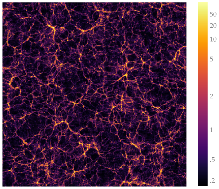
Figure 2: Relative matter density field, $1+\delta$, at $a=1$, projected from an $8\,\mathrm{Mpc}/h$ thick slab in a pmwd simulation, that has evolved $512^{3}$ particles with single precision and a $1024^{3}$ mesh in a $(512\,\mathrm{Mpc}/h)^{3}$ box for 63 time steps. The simulation takes only 13 seconds to finish on an NVIDIA H100 PCIe GPU.

4 Results

We implement the forward simulation and backward adjoint method in the PM code pmwd. All results assume a simple $\Lambda$CDM cosmology: $\bm{\theta}=(A_{\mathrm{s}}=2\times 10^{-9},n_{\mathrm{s}}=0.96,\Omega_{\mathrm{m}}=0.3,\Omega_{\mathrm{b}}=0.05,h=0.7)$, and use an NVIDIA H100 PCIe GPU with 80GB memory.

As in FastPM, the choice of time steps is flexible, and in fact with pmwd it can even be optimized in non-parametric ways to improve simulation accuracy at fixed computation cost. Here we use time steps linearly spaced in scale factor $a$, and leave such optimization in a follow-up work.

4.1 Simulation

We first test the forward simulations of pmwd. Fig. 2 shows the cosmic web in the final snapshot of a fairly large simulation for the size of GPU memories.

Because GPUs are inherently parallel devices, they can output different results for identical inputs. To test the reproducibility, in Table 1 we compare the root-mean-square deviations (RMSDs) of particle displacements and velocities between two runs, relative to their respective standard deviations, with different floating-point precisions, mesh sizes, particle masses, and numbers of time steps. Other than the precision, mesh size is the most important factor, because a finer mesh can better resolve the most nonlinear and dense structures, which can affect reproducibility as the order of many operations can change easily. The particle mass plays a similar role and less massive particles generally take part in nonlinear motions at earlier times. The number of time steps has very small impact except in the most nonlinear cases. And interestingly, more time steps improves the reproducibility most of the time.

Table 1: pmwd reproducibility on GPU. GPUs can output different results for identical inputs. We simulate $384^{3}$ particles from $a=1/64$ to $a=1$, with two floating-point precisions, two mesh sizes, two particle masses (with box sizes of $192\,\mathrm{Mpc}/h$ and $384\,\mathrm{Mpc}/h$), and two time step sizes. We take the root-mean-square deviations (RMSDs) of particle displacements and velocities between two runs at $a=1$, and quote their ratios to the respective standard deviations, about $6\,\mathrm{Mpc}/h$ and $3\times 10^{2}\,\mathrm{km}/\mathrm{s}$. In general, the factors on the left of the left four columns affect the reproducibility more than the those on the right, and lower rows are more reproducible than the upper ones.

precision	cell/ptcl	ptcl mass $[10^{10}M_{\odot}]$	time steps	disp rel diff	vel rel diff
single	8	1	63	$1.6\times 10^{-6}$	$4.8\times 10^{-5}$
single	8	1	126	$5.1\times 10^{-7}$	$1.3\times 10^{-5}$
single	8	8	63	$3.1\times 10^{-7}$	$2.4\times 10^{-6}$
single	8	8	126	$3.1\times 10^{-7}$	$2.3\times 10^{-6}$
single	1	1	63	$1.4\times 10^{-7}$	$1.5\times 10^{-6}$
single	1	1	126	$1.3\times 10^{-7}$	$1.4\times 10^{-6}$
single	1	8	63	$1.1\times 10^{-7}$	$4.5\times 10^{-7}$
single	1	8	126	$9.9\times 10^{-8}$	$4.4\times 10^{-7}$
double	8	1	63	$1.4\times 10^{-15}$	$3.6\times 10^{-14}$
double	8	1	126	$8.3\times 10^{-16}$	$1.7\times 10^{-14}$
double	8	8	63	$5.4\times 10^{-16}$	$4.1\times 10^{-15}$
double	8	8	126	$5.9\times 10^{-16}$	$4.3\times 10^{-15}$
double	1	1	63	$2.4\times 10^{-16}$	$2.3\times 10^{-15}$
double	1	1	126	$2.3\times 10^{-16}$	$2.3\times 10^{-15}$
double	1	8	63	$1.9\times 10^{-16}$	$7.9\times 10^{-16}$
double	1	8	126	$1.8\times 10^{-16}$	$7.8\times 10^{-16}$

4.2 Differentiation

Model differentiation evolves the adjoint equations backward in time. To save memory, the trajectory of the model state in the forward run is not saved, but re-simulated together with the adjoint equations. Even though in principle the $N$-body systems are reversible, in practice the reconstructed trajectory can differ from the forward one due to the finite numerical precision and exacerbated by the chaotic dynamics. Better reversibility means the gradients propagate backward along a trajectory closer to the forward path, and thus would be more accurate. To test this, in Table 2 we compare the RMSDs of the forward-then-reverse particle displacements and velocities from the LPT initial conditions, relative to their respective standard deviations, that are very small at the initial time. As before, we vary the floating-point precision, the mesh size, the particle mass, and the number of time steps. The order of factor importance and their effects are the same as in the reproducibility test. This is because more nonlinear structures are more difficult to reverse. One way to improve reversibility is use higher order LPT to initialize the $N$-body simulations at later times (Michaux et al., 2021), when the displacements and velocities are not as small. We leave this for future development.

Table 2: pmwd reversibility on GPU. Our adjoint method reduces memory cost by reconstructing the forward evolution with reverse time integration. We test the numerical reversibility by comparing the displacements and velocities of particles that have evolved to $a=1$ and then reversed to $a=1/64$, to those of the LPT initial conditions at $a=1/64$, in RMSDs. We take their ratios to the respective standard deviations, about $0.1\,\mathrm{Mpc}/h$ and $0.7\,\mathrm{km}/\mathrm{s}$. Their smallness is the main reason that the quoted relative differences here are orders of magnitude greater than those in Table 1 (see Fig. 3 where the reversibility is few times more important than the reproducibility in their impacts on the gradients). With the same setup as that in Table 1, we see the same general trend—left factors are more important than the right ones, and lower rows are more reversible than the upper ones.

precision	cell/ptcl	ptcl mass $[10^{10}M_{\odot}]$	time steps	disp rel diff	vel rel diff
single	8	1	63	$5.2\times 10^{-2}$	$7.1\times 10^{-2}$
single	8	1	126	$2.1\times 10^{-2}$	$3.6\times 10^{-2}$
single	8	8	63	$3.3\times 10^{-3}$	$7.6\times 10^{-3}$
single	8	8	126	$3.7\times 10^{-3}$	$7.0\times 10^{-3}$
single	1	1	63	$1.4\times 10^{-3}$	$2.2\times 10^{-3}$
single	1	1	126	$1.3\times 10^{-3}$	$1.7\times 10^{-3}$
single	1	8	63	$4.3\times 10^{-4}$	$7.3\times 10^{-4}$
single	1	8	126	$4.4\times 10^{-4}$	$6.3\times 10^{-4}$
double	8	1	63	$5.4\times 10^{-11}$	$1.3\times 10^{-10}$
double	8	1	126	$3.5\times 10^{-11}$	$7.0\times 10^{-11}$
double	8	8	63	$5.8\times 10^{-12}$	$1.4\times 10^{-11}$
double	8	8	126	$6.4\times 10^{-12}$	$1.2\times 10^{-11}$
double	1	1	63	$2.2\times 10^{-12}$	$3.4\times 10^{-12}$
double	1	1	126	$2.1\times 10^{-12}$	$2.9\times 10^{-12}$
double	1	8	63	$7.2\times 10^{-13}$	$1.2\times 10^{-12}$
double	1	8	126	$6.9\times 10^{-13}$	$9.4\times 10^{-13}$

Next, we want to verify that our adjoint method yields the same gradients as those computed by AD. As explained in Sec. 3.6, pmwd already utilizes AD on most of the differentiation tasks. To get the AD gradients we disable our custom VJP implementations on the $N$-body time integration, and the scatter and gather operations. In Fig. 3, we compare the adjoint and AD gradients on a smaller problem, because AD already runs out of memory if we double the number of time steps or increase the space/mass resolution by $2^{3}\times$ from the listed specifications in the caption. For better statistics, we repeat both adjoint and AD runs for 64 times, with the same cosmology and white noise modes, and compare their results by an asymmetric difference of $X_{i}-Y_{j}$, where $1\leq j<i\leq 64$. First we set $X$ and $Y$ to the adjoint and AD gradients respectively, and find they agree very well on the real white noise (so do their gradients on cosmological parameters not shown here; see ). In addition, we can set both $X$ and $Y$ to either adjoint or AD to check their respective reproducibility. We find both gradients are consistent among different runs of themselves, with AD being a lot more reproducible without uncertainty from the reverse time integration but only that from the GPU reproducibility. This implies that we can ignore the reproducibility errors (Table 1) when the reversibility ones dominate (Table 2). Though this statement should be verified again in the future when we reduce the reversibility errors using, e.g., 3LPT.

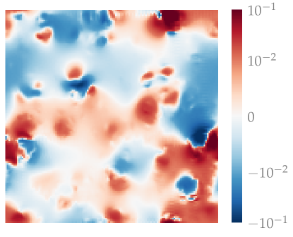
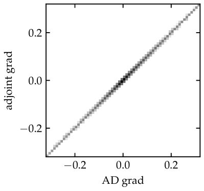
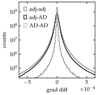
Figure 3: Adjoint gradients of a $128\times 128$ slice of the real white noise field $d\mathcal{J}/d\bm{\omega}$ (top panel), in a pmwd simulation of $128^{3}$ particles in a $(128\,\mathrm{Mpc}/h)^{3}$ box, with a $256^{3}$ mesh, 15 time steps, and single precision. We choose a mean squared error (MSE) objective between two realizations with the same cosmology but different initial modes, on their density fields on the $256^{3}$ mesh at $a=1$, and then compute the gradients with respect to one realization while holding the other fixed. We compare the adjoint gradients to those by AD, for which we have disabled the custom gradient implementation on the scatter, gather, and $N$-body time stepping operators. The adjoint and AD gradients agree as expected, with a RMSD of $\approx 4\times 10^{-5}$, 3 orders of magnitude smaller than the standard deviation of the gradients itself, $\approx 0.015$. It is also comparable to the difference between two different adjoint gradients, with a RMSD $\approx 5\times 10^{-5}$. Different AD gradients are more consistent, with a tighter RMSD of $\approx 1\times 10^{-5}$ due to the absence of uncertainty from reverse time integration.

Our last test on the adjoint gradients uses them in a toy optimization problem in Fig. 4. We use the Adam optimizer (Kingma & Ba, 2015) with a learning rate of $0.1$ and the default values for other hyperparameters. Holding the cosmological parameters fixed, we can optimize the real white noise modes to source initial particles to evolve into our target pattern, in hundreds to thousands of iterations. Interestingly, we find that the variance of the modes becomes bigger than 1 (that of the standard normal white noise) after the optimization, and the optimized modes show some level of spatial correlation not present in the white noise fields, suggesting that the optimized initial conditions are probably no longer Gaussian.

(a) initial conditions at $a=1/64$

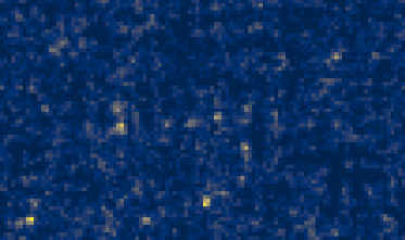
(b) final snapshot at $a=1$

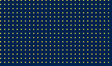
(c) reverse evolution back to $a=1/64$

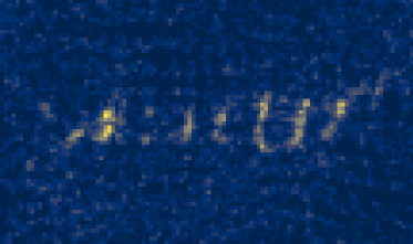
(d) optimization for 10 iterations at $a=1$

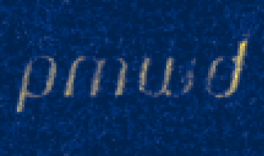
(e) optimization for 100 iterations at $a=1$

(f) optimization for 1000 iterations at $a=1$

Figure 4: A toy problem where we optimize the initial conditions by gradient descent to make some interesting pattern after projection. The particles originally fill a $16\times 27\times 16$ grid, and then evolve from $a=1/64$ to $a=1$ for 63 time steps with single precision and a $32\times 54\times 32$ mesh in a $160\times 270\times 160\,\mathrm{Mpc}^{3}/h^{3}$ box. We compute their projected density in $64\times 108$ pixels and compare that to the target image at the same resolution with an MSE objective. We use the adjoint method and reverse time integration, assuming the latter can reconstruct the forward evolution history accurately. We validate this by demonstrating that the particles evolve backward to align on the initial grid. The optimized initial conditions successfully evolve into the target pattern, which improves with more iterations. Also see the animated reverse time evolution and initial condition optimization on YouTube.

4.3 Performance

pmwd benefits from GPU accelerations and efficient CUDA implementations of scatter and gather operations. In Fig. 5, we present performance test of pmwd, and find both the LPT and the $N$-body parts scale well except for very small problems. The growth function solution has a constant cost, and generally does not affect problem of moderate sizes. However, for a small number of particles and few time steps, it can dominate the computation, in which case one can accelerate the growth computation with an emulator (Kwan et al., 2022).

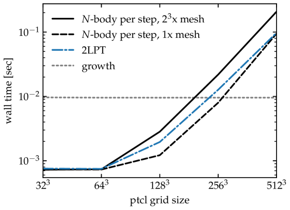
Figure 5: Performance of pmwd. Both the 2LPT and $N$-body components scale well from $512^{3}$ particles to $64^{3}$ particles, below which they become overhead dominated. Solving the growth ODEs takes a constant time, and can dominate the cost for small numbers of particles and few time steps, but generally does not affect problems with more than $128^{3}$ particles.

5 Conclusions

In this work, we develop the adjoint method for memory efficient differentiable cosmological simulations, exploiting the reversible nature of $N$-body Hamiltonian dynamics, and implement it with JAX in a new PM library, pmwd. We have validated the numerical reversibility and the accuracy of the adjoint gradients.

pmwd is both computation and memory efficient, enabling larger and more accurate cosmological dark matter simulations. The next step involves modeling cosmological observables such as galaxies. One can achieve this with analytic, semi-analytic, and deep learning components running based on or in parallel with pmwd. In the future, it can also facilitate the simultaneous modeling of multiple observables and the understanding of the astrophysics at play.

pmwd will benefit all the forward modeling approaches in cosmology, and will improve gradient based optimization and field-level inference to simultaneously constrain the cosmological parameters and the initial conditions of the Universe. The efficiency of pmwd also makes it a promising route to generate the large amount of training data needed by the likelihood-free inference frameworks (Cranmer et al., 2020; Alsing et al., 2019).

Currently, these applications require more development, including distributed parallel capability on multiple GPUs (Modi et al., 2021), more accurate time integration beyond FastPM (List & Hahn, 2023), optimization of spatiotemporal resolution of the PM solvers (Dai & Seljak, 2021; Lanzieri et al., 2022; Zhang et al., in prep), short-range supplement by direct summation of the particle-particle (PP) forces on GPUs (Habib et al., 2016; Potter et al., 2017; Garrison et al., 2021), differentiable models for observables, etc. We plan to pursue these in the future.

Acknowledgements: YL is grateful to all organizers of the 2013 KICP Summer School on Computational Cosmology (Kravtsov et al., 2013), especially Andrey Kravtsov and Nick Gnedin. We thank Alex Barnett, Biwei Dai, Boris Leistedt, ChangHoon Hahn, Daisuke Nagai, Dan Foreman-Mackey, Dan Fortunato, David Duvenaud, David Spergel, Dhairya Malhotra, Erik Thiede, Francisco Villaescusa-Navarro, Fruzsina Agocs, Giulio Fabbian, Jens Stücker, Kaze Wong, Kazuyuki Akitsu, Lehman Garrison, Manas Rachh, Raúl Angulo, Shirley Ho, Simon White, Teppei Okumura, Tomomi Sunayama, Ulrich Steinwandel, Uroš Seljak, Wen Yan, Wenda Zhou, William Coulton, Xiangchong Li, and Yueying Ni for interesting discussions. YL and YZ were supported by The Major Key Project of PCL. YZ was supported by the China Postdoctoral Science Foundation under award number 2023M731831. The Flatiron Institute is supported by the Simons Foundation.

Code Availability: pmwd is open-source on GitHub , including the source files and scripts of this paper . Also see the companion code paper (Li et al., 2022) .

Software: JAX (Bradbury et al., 2018), NumPy (Harris et al., 2020), SciPy (Virtanen et al., 2020), and matplotlib (Hunter, 2007).

Appendix A Growth equations

The 2LPT growth functions follow the following ODEs:

$$D_{1}^{\prime\prime}+\Bigl{(}2+\frac{H^{\prime}}{H}\Bigr{)}D_{1}^{\prime}-\frac{3}{2}\Omega_{\mathrm{m}}(a)D_{1} =0,$$

$$D_{2}^{\prime\prime}+\Bigl{(}2+\frac{H^{\prime}}{H}\Bigr{)}D_{2}^{\prime}-\frac{3}{2}\Omega_{\mathrm{m}}(a)D_{2} =\frac{3}{2}\Omega_{\mathrm{m}}(a)D_{1}^{2},$$ (A1)

where

$$\Omega_{\mathrm{m}}(a)=\frac{\Omega_{\mathrm{m}}H_{0}^{2}}{a^{3}H^{2}}$$ (A2)

If the universe has been sufficiently matter dominated at $a_{\mathrm{i}}$, with $\Omega_{\mathrm{m}}(a_{\mathrm{i}})\simeq 1$ and $H^{\prime}/H\simeq-3/2$, the initial conditions of the ODEs can be set as the growing mode in this limiting case

$$D_{1}(a_{\mathrm{i}}) =a_{\mathrm{i}},$$

$$D_{1}^{\prime}(a_{\mathrm{i}}) =a_{\mathrm{i}},$$

$$D_{2}(a_{\mathrm{i}}) =\frac{3}{7}a_{\mathrm{i}}^{2},$$

$$D_{2}^{\prime}(a_{\mathrm{i}}) =\frac{6}{7}a_{\mathrm{i}}^{2}.$$ (A3)

$D_{1}\simeq a$ in the matter dominated era, before being suppressed by dark energy.

The above growth equations can be written in such suppression factors,

$$G_{m}\triangleq D_{m}/a^{m},$$ (A4)

for $m\in\{1,2\}$, as

$$G_{1}^{\prime\prime}+\Bigl{(}4+\frac{H^{\prime}}{H}\Bigr{)}G_{1}^{\prime}+\Bigl{(}3+\frac{H^{\prime}}{H}-\frac{3}{2}\Omega_{\mathrm{m}}(a)\Bigr{)}G_{1} =0,$$

$$G_{2}^{\prime\prime}+\Bigl{(}6+\frac{H^{\prime}}{H}\Bigr{)}G_{2}^{\prime}+\Bigl{(}8+2\frac{H^{\prime}}{H}-\frac{3}{2}\Omega_{\mathrm{m}}(a)\Bigr{)}G_{2} =\frac{3}{2}\Omega_{\mathrm{m}}(a)G_{1}^{2},$$ (A5)

with initial conditions

$$G_{1}(a_{\mathrm{i}}) =1,$$

$$G_{1}^{\prime}(a_{\mathrm{i}}) =0,$$

$$G_{2}(a_{\mathrm{i}}) =\frac{3}{7},$$

$$G_{2}^{\prime}(a_{\mathrm{i}}) =0.$$ (A6)

We solve the growth equations in $G_{m}$ instead of $D_{m}$, with the JAX adaptive ODE integrator implementing the adjoint method in the optimize-then-discretize approach. This is because the former can be integrated backward in time more accurately for early times, which can improve the adjoint gradients.

We can then evaluate the FastPM time integration factors in (14) by

$$G_{D} =a^{2}\dot{D}_{1}=a^{2}HD_{1}^{\prime},$$

$$G_{K} =a\dot{G}_{D}=a^{3}H^{2}\Bigl{[}D_{1}^{\prime\prime}+\Bigl{(}2+\frac{H^{\prime}}{H}\Bigr{)}D_{1}^{\prime}\Bigr{]},$$ (A7)

and

$$D_{m} =a^{m}G_{m}$$

$$D_{m}^{\prime} =a^{m}\bigl{(}mG_{m}+G_{1}^{\prime}\Bigr{)},$$

$$D_{m}^{\prime\prime} =a^{m}\bigl{(}m^{2}G_{1}+2mG_{1}^{\prime}+G_{1}^{\prime\prime}\Bigr{)}.$$ (A8)

References

• Alsing et al. (2019) Alsing, J., Charnock, T., Feeney, S., & Wandelt, B. 2019, Monthly Notices of the Royal Astronomical Society, 488, 4440
• Angulo & Hahn (2022) Angulo, R. E., & Hahn, O. 2022, Living Reviews in Computational Astrophysics, 8, 1, doi: 10.1007/s41115-021-00013-z
• Blas et al. (2011) Blas, D., Lesgourgues, J., & Tram, T. 2011, Journal of Cosmology and Astroparticle Physics, 2011, 034
• Böhm et al. (2021) Böhm, V., Feng, Y., Lee, M. E., & Dai, B. 2021, Astronomy and Computing, 36, 100490
• Bouchet et al. (1995) Bouchet, F. R., Colombi, S., Hivon, E., & Juszkiewicz, R. 1995, Astronomy and Astrophysics, 296, 575. https://arxiv.org/abs/astro-ph/9406013
• Bradbury et al. (2018) Bradbury, J., Frostig, R., Hawkins, P., et al. 2018, JAX: Composable Transformations of Python+Numpy Programs: Differentiate, Vectorize, JIT to GPU/TPU, and More. http://github.com/google/jax
• Bradley (2019) Bradley, A. M. 2019. https://cs.stanford.edu/~ambrad/adjoint_tutorial.pdf
• Chen et al. (2018) Chen, R. T. Q., Rubanova, Y., Bettencourt, J., & Duvenaud, D. K. 2018, in Advances in Neural Information Processing Systems 31, ed. S. Bengio, H. Wallach, H. Larochelle, K. Grauman, N. Cesa-Bianchi, & R. Garnett (Curran Associates, Inc.), 6571–6583. http://papers.nips.cc/paper/7892-neural-ordinary-differential-equations.pdf
• Cranmer et al. (2020) Cranmer, K., Brehmer, J., & Louppe, G. 2020, Proceedings of the National Academy of Sciences, 117, 30055, doi: 10.1073/pnas.1912789117
• Dai & Seljak (2021) Dai, B., & Seljak, U. 2021, Proceedings of the National Academy of Sciences, 118, e2020324118
• Eisenstein & Hu (1998) Eisenstein, D. J., & Hu, W. 1998, The Astrophysical Journal, 496, 605
• Feng (2017) Feng, Y. 2017, Automatic Differentiation and Cosmology Simulation. https://bids.berkeley.edu/news/automatic-differentiation-and-cosmology-simulation
• Feng (2018) —. 2018, vmad: A Simple Autodiff and a Small Library of Operators. https://github.com/rainwoodman/vmad
• Feng et al. (2016) Feng, Y., Chu, M.-Y., Seljak, U., & McDonald, P. 2016, Monthly Notices of the Royal Astronomical Society, 463, 2273, doi: 10.1093/mnras/stw2123
• Garrison et al. (2021) Garrison, L. H., Eisenstein, D. J., Ferrer, D., Maksimova, N. A., & Pinto, P. A. 2021, Monthly Notices of the Royal Astronomical Society, 508, 575, doi: 10.1093/mnras/stab2482
• Gholaminejad et al. (2019) Gholaminejad, A., Keutzer, K., & Biros, G. 2019, in Proceedings of the Twenty-Eighth International Joint Conference on Artificial Intelligence, IJCAI-19 (International Joint Conferences on Artificial Intelligence Organization), 730–736, doi: 10.24963/ijcai.2019/103
• Griewank & Walther (2000) Griewank, A., & Walther, A. 2000, ACM Transactions on Mathematical Software (TOMS), 26, 19
• Habib et al. (2016) Habib, S., Pope, A., Finkel, H., et al. 2016, New Astronomy, 42, 49
• Harris et al. (2020) Harris, C. R., Millman, K. J., van der Walt, S. J., et al. 2020, Nature, 585, 357, doi: 10.1038/s41586-020-2649-2
• Hockney & Eastwood (1988) Hockney, R. W., & Eastwood, J. W. 1988, Computer Simulation Using Particles (USA: Taylor & Francis, Inc.)
• Hunter (2007) Hunter, J. D. 2007, Computing in Science & Engineering, 9, 90, doi: 10.1109/MCSE.2007.55
• Jasche & Lavaux (2019) Jasche, J., & Lavaux, G. 2019, Astronomy & Astrophysics, 625, A64, doi: 10.1051/0004-6361/201833710
• Jasche & Wandelt (2013) Jasche, J., & Wandelt, B. D. 2013, Monthly Notices of the Royal Astronomical Society, 432, 894, doi: 10.1093/mnras/stt449
• Kingma & Ba (2015) Kingma, D. P., & Ba, J. 2015, in 3rd International Conference on Learning Representations, ICLR 2015, San Diego, CA, USA, May 7-9, 2015, Conference Track Proceedings, ed. Y. Bengio & Y. LeCun. https://arxiv.org/abs/1412.6980
• Kravtsov et al. (2013) Kravtsov, A. V., Gnedin, N. Y., Habib, S., & Heitmann, K. 2013, KICP Summer School: Computational Cosmology | CompCosmology 2013. https://kicp-workshops.uchicago.edu/compcosmology2013/
• Kwan et al. (2022) Kwan, N. P., Modi, C., Li, Y., & Ho, S. 2022, in NeurIPS 2022 Machine Learning and the Physical Sciences. https://arxiv.org/abs/2211.06564
• Lanzieri et al. (2022) Lanzieri, D., Lanusse, F., & Starck, J.-L. 2022, Machine Learning for Astrophysics Workshop at the Thirty-ninth International Conference on Machine Learning (ICML 2022). http://arxiv.org/abs/2207.05509
• Lewis & Challinor (2011) Lewis, A., & Challinor, A. 2011, Astrophysics source code library, ascl
• Li et al. (2022) Li, Y., Lu, L., Modi, C., et al. 2022, to be submitted to Journal of Open Source Software. https://arxiv.org/abs/2211.09958
• List & Hahn (2023) List, F., & Hahn, O. 2023, Perturbation-Theory Informed Integrators for Cosmological Simulations, arXiv, doi: 10.48550/arXiv.2301.09655
• Michaux et al. (2021) Michaux, M., Hahn, O., Rampf, C., & Angulo, R. E. 2021, Monthly Notices of the Royal Astronomical Society, 500, 663, doi: 10.1093/mnras/staa3149
• Modi et al. (2021) Modi, C., Lanusse, F., & Seljak, U. 2021, Astronomy and Computing, 37, 100505, doi: 10.1016/j.ascom.2021.100505
• Pontryagin (1962) Pontryagin, L. S. 1962, The Mathematical Theory of Optimal Processes (CRC press)
• Potter et al. (2017) Potter, D., Stadel, J., & Teyssier, R. 2017, Computational Astrophysics and Cosmology, 4, doi: 10.1186/s40668-017-0021-1
• Quinn et al. (1997) Quinn, T., Katz, N., Stadel, J., & Lake, G. 1997. https://arxiv.org/abs/astro-ph/9710043
• Seljak et al. (2017) Seljak, U., Aslanyan, G., Feng, Y., & Modi, C. 2017, Journal of Cosmology and Astroparticle Physics, 2017, 009, doi: 10.1088/1475-7516/2017/12/009
• Virtanen et al. (2020) Virtanen, P., Gommers, R., Oliphant, T. E., et al. 2020, Nature Methods, 17, 261, doi: 10.1038/s41592-019-0686-2
• Wang et al. (2014) Wang, H., Mo, H. J., Yang, X., Jing, Y. P., & Lin, W. P. 2014, The Astrophysical Journal, 794, 94, doi: 10.1088/0004-637X/794/1/94
• Zhang et al. (in prep) Zhang, Y., Li, Y., Jamieson, D., Lu, L., & et al. in prep