Data-driven Real-time Short-term Prediction of Air Quality: Comparison of ES, ARIMA, and LSTM

Abstract

Air pollution is a worldwide issue that affects the lives of many people in urban areas. It is considered that the air pollution may lead to heart and lung diseases. A careful and timely forecast of the air quality could help to reduce the exposure risk for affected people. In this paper, we use a data-driven approach to predict air quality based on historical data. We compare three popular methods for time series prediction: Exponential Smoothing (ES), Auto-Regressive Integrated Moving Average (ARIMA) and Long short-term memory (LSTM). Considering prediction accuracy and time complexity, our experiments reveal that for short-term air pollution prediction ES performs better than ARIMA and LSTM.

ir pollution, Exponential Smoothing, ARIMA, LSTM

1 Introduction

The high-density of urban population may often lead to high-levels of various kinds of pollution, such as, air pollution [25], light pollution [11], or noise pollution[2, 3]. Air pollution is an important indicator of the life quality of a city. It may affect human health by causing heart and lung diseases [7]. Furthermore, air pollution is a significant contributor to climate change [19]. Table 1 describes the health impact of some of the most harmful air pollutants.

Table 1: Impact of air pollution on human health.

Pollutant	Health Impact
CO	Mostly affects the cardiovascular system and leads to a lack of oxygen in the human body. The outcome is bad concentration and slow reflexes. It also may cause lung inflammation.
O3	Affects lungs and respiratory system and may lead to lung inflammation. It also reduces lung functions and may cause asthma or even lung cancer.
NO2, SO2	Affects the respiratory system by reducing its resistance to respiratory infections.
PM	May cause inflammatory lung changes. It is dangerous due to its small size, which allows it to reach the heart and the brain and may cause inflammation there.

Sensors for personal use enable to measure the air pollution at a specific location. Based on the retrieved data, it is possible to predict future air pollution using time series forecasting methods. Existing solutions, are already capable to quantify the air quality state. However, these solutions do not provide short-term forecasts in real time.

Prediction of time series in near real time implies that the model should be periodically updated to account for recently generated data. Amjad et al. [5] propose to monitor the trend of the financial time series and update the model if the trend changes direction. Qin et al. [18] suggest to create a schedule for updating the data within fixed time frame. For an adaptive model selection, Le et al. [10] suggest to update the model each time new data arrives. A trend in the series of air pollution data may change unpredictably because of environmental changes. Therefore, updating the model each time new data arrives is a promising approach for air pollution data.

In this paper, we compare methods that may be applied to real-time prediction of air quality. We conduct a performance comparison with respect to the prediction accuracy and time complexity for three methods: Exponential Smoothing, ARIMA, and LSTM. For experimental evaluation we use a data set [16] that comprises air pollution data collected in Skopje. Our experimental results indicate that Exponential Smoothing outperforms ARIMA and LSTM for real time prediction of air quality.

The rest of the paper is structured as follows. We describe the data set, code implementation, and metrics in Section 2. Section 3 describes the experimental evaluation. Related work is discussed in Section 4. Section 5 concludes the paper.

2 Methodology

In this section, we describe data preparation, code implementation of prediction methods, and metrics.

2.1 Data preparation

We use for experimental evaluation the data collected in Skopje [16]. This data set contains air pollution measurements from seven stations, and includes CO, NO2, O3, PM10, and PM2.5. The pollutants behave quite similar over time, and our focus in this study is on PM2.5.

Figure 1 visualizes the data set that originally had missing values and outliers.

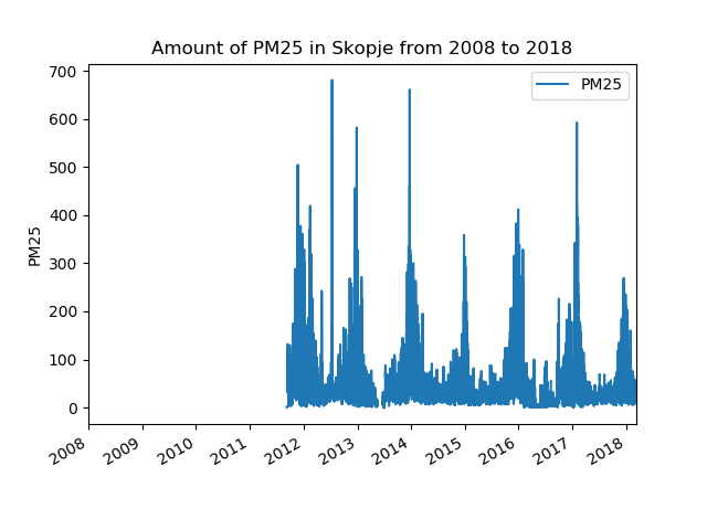
Figure 1: Initial data set.

We use linear interpolation for filling missing values. It is assumed that missing values lie on the line which could be drawn using a set of known points. The data set after applying interpolation is depicted in Figure 2.

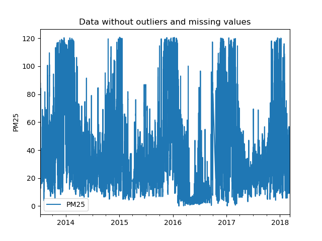
Figure 2: Data set after filling missing values.

Because we are interested in short-term predictions, we decided to predict the air pollution 24 hours ahead; that is, the test interval is 24 hours. In accordance with [21] the training and test interval are split as 70% and 30% respectively. We should consider that the prediction accuracy of a Neural Network usually improves with the increase of the amount of training data. Therefore, for the LSTM model the training set is much larger than for statistical models.

2.2 Code implementation

We have implemented all algorithms in this study in Python using open source libraries and frameworks (including, statsmodels [12], pmdarima [22], keras [8], tensorflow [1]).

2.3 Measurement metrics

For the real-time environment emulation, we use the rolling window technique. After building the model and making the forecast, the data is moved one hour ahead and model building and forecasting is repeated.

Figure 3 depicts the rolling forecast. The forecast is done multiple times using different data and the error is calculated by averaging all errors that we have got. This technique is independent of the data and provides correct results.

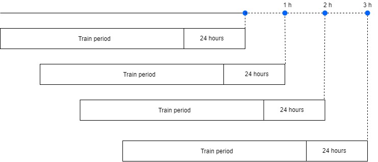
Figure 3: Rolling forecast enables to emulate the real-time environment.

We use the Root Mean Squared Error (RMSE), because it is considered to be less sensitive with respect to outliers. RMSE is the square root of the average of squared differences between the predicted value and actual value of the series.

$$RMSE=\sqrt{\frac{\sum_{t=1}^{n}(y_{i}-x_{i})^{2}}{n}}$$ (1)

All experiments were conducted multiple times on different time intervals and the mean of the results has been taken. Also for each method, the multi-step forecast has been produced for comparison.

3 Evaluation

In this section, we present the training intervals and the Root Mean Squared Error (RMSE) for Exponential Smoothing, ARIMA, and LSTM. Additionally, a performance comparison of the studied methods is provided.

3.1 Exponential smoothing (ES)

To determine the best training intervals we conducted the following experiment. We have trained the model for various numbers of hours and selected the one that resulted with the lowest RMSE. Because we are aiming for short-term predictions, it is not necessary to consider larger training intervals.

Table 2 presents the average RMSE for different training intervals. We may observe that the best training interval for Exponential Smoothing is 96 hours, because RMSE for this period is the lowest.

Table 2: RMSE of ES model for various training intervals.

Time [h]	48	72	96	120	144	168	196
RMSE	10.54	9.76	6.39	8.26	10.47	12.6	10.12

3.2 ARIMA

To make the prediction process faster and reduce the model selection time an experiment for determining hyperparameter intervals has been conducted. We have evaluated various time intervals to determine what the minimum and maximum values of the hyperparameters could be. The results of this experiment are presented in Table 3.

Table 3: ARIMA hyperparameter intervals.

Hyperparameter	Minimum	Maximum
p	0	6
d	0	2
q	0	5
P	0	3
D	0	1
Q	0	2

After the hyperparameters boundaries were determined, we observed a significant improvement in the speed of building an ARIMA model.

Table 4 indicates that the best training interval for the ARIMA model is 120 hours, because it results with the lowest RMSE across the considered intervals.

Table 4: RMSE of ARIMA model for various training intervals

Time [h]	72	96	120	144	168	196	220
RMSE	11.24	8.89	8.59	12.1	14.32	12.83	11.56

The time for building the ARIMA model and performing prediction is 19.8 seconds in our experiment. While the time required for building ARIMA model and performing prediction is shorter than for Exponential Smoothing (20.5 seconds), the prediction error of ARIMA model is larger.

3.3 LSTM

We have implemented LSTM using Keras framework [8]. In the first stage of the experiment, we evaluated different LSTM configurations: Simple, Stacked, Bidirectional, and Encoder-decoder.

Table 5: Accuracy and execution time of various LSTM network configurations.

Network Configuration	RMSE	Time [s]
Simple	3.26	1196.32
Stacked	3.32	1253.21
Bidirectional	4.19	1372.65
Encoder-decoder	3.75	1476.87

Evaluation results of LSTM network configurations are presented in Table 5. We may observe that the best accuracy is achieved using a Simple LSTM configuration. In what follows in this section, we describe experimental results for the Simple LSTM configuration. Table 6 shows the selected values of hyperparameters for the Simple LSTM configuration.

Table 6: LSTM hyperparameter values.

Hyper-parameter	Value
Epoch	800
Patience coefficient	0.1
Validation size	72 hours
Dropout	0.1
Recurrent dropout	0.3
Batch size	12
Type	Statefull
Coefficient for counting units	3
Training size	8000

Table 7 shows RMSE and execution time of the Simple LSTM configuration for various values of prediction horizon.

We may observe that the execution time of LSTM is significantly higher than for the other methods considered in this study (that is, ES and ARIMA). Furthermore, the prediction accuracy worsens with the increase of the prediction horizon.

Table 7: RMSE and execution time of the Simple LSTM configuration for various values of Horizon.

Horizon [h]	RMSE	Time [s]
1	3.26	1282.46
2	4.47	953.40
3	5.35	1140.42
4	6.17	1185.93
5	7.07	1101.65
6	7.31	967.06
7	8.24	1303.88
8	6.21	900.61
9	9.06	1111.17
10	9.14	1055.00
11	9.67	1354.31
12	10.41	1081.18
13	10.44	1258.37
14	11.06	1195.12
15	10.71	936.59
16	11.29	1107.04
17	11.88	1213.67
18	13.40	1155.57
19	12.02	977.91
20	12.55	966.46
21	12.71	1199.05
22	12.93	1078.39
23	11.74	1003.03
24	14.69	1117.89

3.4 Performance comparison of ES, ARIMA, and LSTM

Figure 4 depicts the relationship of RMSE and prediction horizon for ES, ARIMA, and LSTM. RMSE increases for all three considered methods with the increase of prediction horizon. For all considered values of prediction horizon, ES has the lowest RMSE (that is, the highest prediction accuracy) compared to ARIMA and LSTM.

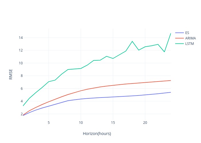
Figure 4: RMSE and prediction Horizon [h] for ES, ARIMA, and LSTM.

With respect to the time for building a model and making a forecast, ARIMA and ES require about 20 seconds in our experiments. LSTM is significantly slower and requires about 1000 seconds for model building and forecasting.

Considering prediction accuracy (that is, RMSE) and model building and forecasting time, we may conclude that ES is the most suitable among the studied methods for short-term prediction of air pollution.

3.5 Future research directions

The future work may investigate the performance of additional prediction methods in the context of air pollution. Techniques for parallel processing ([4, 17]), acceleration ([24, 13, 6]), and intelligent parameter selection ([14]) could be studied to further improve the efficiency.

4 Related Work

In this section, we provide an overview of the related work.

Shaban et al. [20] investigate three machine learning algorithms that could be used for alarming applications in the context of air pollution: Support Vector Machines, M5P Model Trees, and Artificial Neural Networks. In future they plan to study real-time prediction of air pollution.

Subramanian [23] studies application of Multiple Linear Regression and Neural Networks to forecasting of the pollution concentration.

Le et al. [9] describe an air-pollution prediction model that is based on spatio-temporal data that is collected from air quality sensors installed on taxis running across the city Daegu, Korea. The prediction model is based on the Convolutional Neural Network for an image like spatial distribution of air pollution. The temporal information in the data is handled using a combination of a Long Short-Term Memory unit for time series data and a Neural Network model for other air pollution impact factors (such as, weather conditions.)

Ochando et al. [15] use traffic and weather data for prediction of the air pollution. The aim is to provide general information about the air quality of the city, and they do not focus on a particular spot within the city. In this study, the Random Forest model performs best.

Related work mostly focuses on studying air pollution data that has been already generated and stored in the past. In contrast to related work, we focus on using continuously updated data (that may be generated by sensors) for short-term prediction of the air pollution in near real-time.

5 Conclusions

We have presented various methods that may be applied to short-term air quality prediction in real time. Using a real-world data set we conducted a performance comparison of three methods: Exponential Smoothing, ARIMA, and LSTM.

We have observed that Exponential Smoothing performs more efficiently for the short-term air pollution prediction compared to ARIMA and LSTM. LSTM has larger prediction error and takes more time to make the prediction. For the multi-step ahead forecast the gap between prediction errors of these methods grows with the increase of the number of steps.

References

- [1] Abadi, M., Barham, P., Chen, J., Chen, Z., Davis, A., Dean, J., Devin, M., Ghemawat, S., Irving, G., Isard, M., et al.: Tensorflow: A system for large-scale machine learning. In: 12th USENIX Symposium on Operating Systems Design and Implementation (OSDI 16). pp. 265–283 (2016)
- [2] Alsouda, Y., Pllana, S., Kurti, A.: A Machine Learning Driven IoT Solution for Noise Classification in Smart Cities. In: Machine Learning Driven Technologies and Architectures for Intelligent Internet of Things (ML-IoT). pp. 1–6. Euromicro (2018). https://doi.org/10.48550/arXiv.1809.00238
- [3] Alsouda, Y., Pllana, S., Kurti, A.: IoT-based Urban Noise Identification Using Machine Learning: Performance of SVM, KNN, Bagging, and Random Forest. In: Proceedings of the International Conference on Omni-Layer Intelligent Systems. pp. 62–67. COINS ’19, ACM, New York, NY, USA (2019). https://doi.org/10.1145/3312614.3312631
- [4] Amaral, V., Norberto, B., Goulão, M., Aldinucci, M., Benkner, S., Bracciali, A., Carreira, P., Celms, E., Correia, L., Grelck, C., Karatza, H., Kessler, C., Kilpatrick, P., Martiniano, H., Mavridis, I., Pllana, S., Respício, A., Simão, J., Veiga, L., Visa, A.: Programming languages for data-intensive HPC applications: A systematic mapping study. Parallel Computing 91, 102584 (2020). https://doi.org/https://doi.org/10.1016/j.parco.2019.102584
- [5] Amjad, M., Shah, D.: Trading bitcoin and online time series prediction. In: NIPS 2016 Time Series Workshop. pp. 1–15 (2017)
- [6] Benkner, S., Pllana, S., Traff, J., Tsigas, P., Dolinsky, U., Augonnet, C., Bachmayer, B., Kessler, C., Moloney, D., Osipov, V.: PEPPHER: Efficient and Productive Usage of Hybrid Computing Systems. IEEE Micro 31(5), 28–41 (2011). https://doi.org/10.1109/MM.2011.67
- [7] Das, P.K., A, D.V., Meher, S., Panda, R., Abraham, A.: A systematic review on recent advancements in deep and machine learning based detection and classification of acute lymphoblastic leukemia. IEEE Access 10, 81741–81763 (2022). https://doi.org/10.1109/ACCESS.2022.3196037
- [8] Gulli, A., Pal, S.: Deep Learning with Keras. Packt Publishing Ltd (2017)
- [9] Le, D.: Real-time air pollution prediction model based on spatiotemporal big data. arXiv preprint arXiv:1805.00432 (2018)
- [10] Le Borgne, Y.A., Santini, S., Bontempi, G.: Adaptive model selection for time series prediction in wireless sensor networks. Signal Processing 87(12), 3010–3020 (2007)
- [11] Longcore, T., Rich, C.: Ecological light pollution. Frontiers in Ecology and the Environment 2(4), 191–198 (2004)
- [12] Massaron, L., Boschetti, A.: Regression Analysis with Python. Packt Publishing Ltd (2016)
- [13] Memeti, S., Pllana, S.: Accelerating DNA Sequence Analysis Using Intel(R) Xeon Phi(TM). In: 2015 IEEE Trustcom/BigDataSE/ISPA. vol. 3, pp. 222–227 (2015). https://doi.org/10.1109/Trustcom.2015.636
- [14] Memeti, S., Pllana, S.: Optimization of heterogeneous systems with AI planning heuristics and machine learning: a performance and energy aware approach. Computing 103(12), 2943–2966 (Dec 2021). https://doi.org/10.1007/s00607-021-01017-6
- [15] Ochando, L.C., Julián, C.I.F., Ochando, F.C., Ferri, C.: Airvlc: An application for real-time forecasting urban air pollution. In: Proceedings of the 2nd International Conference on Mining Urban Data - Volume 1392. p. 72–79. MUD’15, CEUR-WS.org, Aachen, DE (2015)
- [16] Petrushevski, S.: Air pollution in Skopje from 2008 to 2018 (2018), https://www.kaggle.com/cokastefan/pm10-pollution-data-in-skopje-from-2008-to-2018
- [17] Pllana, S., Xhafa, F.: Programming Multicore and Many-core Computing Systems. John Wiley & Sons, Inc., Hoboken, New Jersey, USA, 1 edn. (2017). https://doi.org/10.1002/9781119332015
- [18] Qin, X., Mahmassani, H.S.: Adaptive calibration of dynamic speed-density relations for online network traffic estimation and prediction applications. Transportation research record 1876(1), 82–89 (2004)
- [19] Seinfeld, J.H., Pandis, S.N.: Atmospheric chemistry and physics: from air pollution to climate change. John Wiley & Sons (2016)
- [20] Shaban, K.B., Kadri, A., Rezk, E.: Urban air pollution monitoring system with forecasting models. IEEE Sensors Journal 16(8), 2598–2606 (April 2016). https://doi.org/10.1109/JSEN.2016.2514378
- [21] Siami-Namini, S., Namin, A.S.: Forecasting economics and financial time series: Arima vs. lstm. arXiv preprint arXiv:1803.06386 (2018)
- [22] Smith, T.G.: pmdarima: Arima estimators for Python (2017)
- [23] Subramanian, V.N.: Data analysis for predicting air pollutant concentration in smart city uppsala (2016)
- [24] Viebke, A., Memeti, S., Pllana, S., Abraham, A.: CHAOS: a parallelization scheme for training convolutional neural networks on Intel Xeon Phi. The Journal of Supercomputing 75(1), 197–227 (Jan 2019). https://doi.org/10.1007/s11227-017-1994-x
- [25] Yang, D., Wang, J., Yan, X., Liu, H.: Subway air quality modeling using improved deep learning framework. Process Safety and Environmental Protection 163, 487–497 (2022). https://doi.org/https://doi.org/10.1016/j.psep.2022.05.055