Scattering entropies of quantum graphs with several channels
Abstract
This work deals with the scattering entropy of quantum graphs in many different circumstances. We first consider the case of the Shannon entropy, and then the Rényi and Tsallis entropies, which are more adequate to study distinct quantitative behavior such as entanglement and nonextensive behavior, respectively. We describe many results, associated with different types of quantum graphs in the presence of several vertices, edges and leads. In particular, we emphasize that the results may be used as quantifiers of diversity or nonadditivity, related to the transport in quantum graphs.
keywords:
Graphs , Scattering , Entropy , Rényi entropy , Tsallis entropy1 Introduction
Entropies are in general used to work as quantifies of diversity, uncertainty, or randomness of a given system. In this sense, investigations utilizing the concept of entropy have been considered in many different areas of nonlinear science. Among the several distinct possibilities, in this work, we will consider entropies introduced by Shannon, Rényi and Tsallis related to quantum graphs. Quantum graphs are nicely studied in Ref. [1], and the associated entropies will be introduced below, connecting them with statistical information.
As one knows, the Shannon entropy [2] is directly connected to information in general, and it can be seen as a way to express probability. The Rényi entropy, on the other hand, can be seen as an index of diversity and in this sense be directly related to ecology, economy and statistics, for instance, where it intends to provide a quantitative measure to account for the many different types of species or objects there are in a community or dataset. It is also connected with entanglement measures in a quantum system, and in this case, it has been recently used in many different contexts in high energy physics; see, e.g., Refs.[3, 4, 5, 6] and references therein, and the results on charged Rényi entropies [7, 8]. The Tsallis entropy [9, 10] is of interest to investigate systems where nonextensive or nonadditive behavior plays an important role. The concept has been used to investigate physical behavior in several distinct areas; see, e.g. [11] where hadron spectra can be adequately described by nonextensive statistical mechanical distribution and also, the recent works on black hole entropy [12] and nonlinear wave propagation in relativistic quark-gluon plasma [13].
In the present work, we shall further explore the use of the Shannon entropy to quantify scattering in simple quantum graphs, as we have studied before in [14, 15]. Here, however, we shall expand our investigation into two distinct directions: first, we study the Shannon entropy associated to scattering in simple quantum graphs in terms of the energy of the incoming signal, and not only in the form of the average quantity that we have introduced before. The second line of investigation concerns the extension of the concept of the Shannon entropy to the cases of the Rényi and Tsallis entropies, which are supposed to be more appropriate to investigate systems with distinct statistical contents, such as entanglement measures and nonextensive behavior. Since we do not know in principle how a quantum graph arrangement may respond under the Shannon, Rényi or Tsallis entropies, we think it is worth studying these possibilities, to see if we can quantify the different behavior they certainly engender.
The study of the Shannon entropy intended to introduce another quantifier of information in simple quantum graphs was first presented in Refs. [14, 15]. It was inspired by the possibility to add a global quantifier associated with a scattering process in a quantum graph. In other areas of research, it was also motivated by several interesting results, in particular, on the possibility to make the energy flux travel from a cold system to a hot system, by increasing the Shannon entropy of the memory to compensate for the decrease in the thermodynamic entropy [16], and on the theoretical framework for the thermodynamics of information, connected to stochastic thermodynamics and fluctuation theorems, opening a way to manipulate information at the molecular or nanometric scales [17]. Moreover, in high-energy physics, the concept of configurational entropy, based on the Shannon entropy, was first introduced in [18, 19]. It has also been used in some interesting directions to examine stability of physical systems such as in the investigation of glueballs [20], heavy mesons [21] and skyrmions [22, 23], the configurational entropy in AdS/QCD models [24, 25], entanglement generation in meson-meson scattering process [26] , the nuclear information entropy [27, 28], and in other scenarios of recent interest [29, 30].
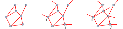
To describe the present investigation pedagogically, we organize the work as follows. In Sec. 2 we review two important issues, one being the scattering in quantum graphs, and the other the concept of Shannon entropy associated to the quantum scattering, and then we add the extensions to the case of Rényi and Tsallis entropies. To investigate the scattering one needs to make the quantum graph open, and we do this by attaching leads to vertices in the graph, as it is illustrated in the case of a graph with 7 vertices and 10 edges in Fig. 1. In the same Sec. 2, we implement the main novelties of the work, which concerns the calculations related to the Shannon, Rényi and Tsallis entropies and we do this for both the scattering entropy, which depend on the energy or the wave number of the incoming signal, and the average scattering entropies, which are global quantities, averaged over the period of the periodic scattering probabilities. We then move on to illustrate the results with several distinct examples, for the Shannon, Rényi and Tsallis entropies. This is implemented in Sec. 3, where we compute the results for series and parallel disposition of vertices, and also for the following types of graphs: cycle, wheel and complete graphs. We compare some results, to show how these different quantities behave as we vary the energy or wave number of the incoming signal in the quantum graph.
2 Scattering and entropies in quantum graphs
The interest in quantum graphs started with the studies of Kottos and Smilansky [31, 32] in the context of quantum chaos, where they analyzed the spectral statistics of simple quantum graphs and showed that the spectra closely follows the prediction of the random matrix theory. An important result from the studies of quantum graphs is the possibility of obtaining analytical solutions even when they present chaotic behavior [33, 34, 35, 36]. The spectral analysis in graphs is still of current interest [37], and quantum graphs are deeply related to the concept of quantum walks [38] as discussed by Tanner in Ref. [39]. Since quantum walks are the quantum version of the classical random walks, the case of classical random walks is also of interest. As one knows, classical random walks are diffusive, so diffusion in graphs and networks is also of current interest [40] and may be investigated using quantifiers of entropy as well.
In order to develop our investigation, we recall that, mathematically, a simple quantum graph, , consists of (i) a metric graph, i.e., a set of vertices, , and a set of edges, , where each edge is a pair of vertices , and we assign positive lengths to each edge .; (ii) a differential operator, ; and (iii) a set of boundary conditions (BC) at the vertices of the graph [1]. Thus we say that a quantum graph is a triple . In this work, we consider the free Schrödinger operator on each edge and Neumann boundary conditions on the vertices. The graph topology is totally defined by its adjacency matrix of dimension , whose elements are given by
| (1) |
where means that the vertex is adjacent to . We create an open quantum graph, , which is suitable to study scattering problems, by adding leads (semi-infinite edges) to its vertices (see Fig. 1). The open quantum graph then represents a scattering system with scattering channels which is characterized by the energy dependent global scattering matrix , where is the wave number and the matrix elements are given by the scattering amplitudes , where and are the entrance and exit scattering channels, respectively.
In this work, we employ the Green’s function approach as developed in Refs. [41, 42] to determine the scattering amplitudes . This technique was used to study narrow peaks of full transmission and transport in simple quantum graphs [43, 44], and the scattering Shannon entropy for quantum graphs [15, 14]. These latter ones have inspired us to describe the present study. The exact scattering Green’s function for a quantum particle of wave number entering the graph at the vertex and exiting at the vertex is given by
| (2) |
where
| (3) |
In Eq. (2), and are reference points on the leads connected to the vertices and , respectively. In Eq. (3), is the set of neighbor vertices connected to , and () is the -dependent reflection (transmission) amplitude at the vertex , which is determined unambiguously from the BC. The so-called family of paths between the vertices and , are given by
| (4) |
where with being the length of the edge connecting and , and being the set of neighbors vertices of but with the vertices and excluded. The family can be obtained from the above equation by swapping , and the number of family of paths is always twice the number of edges in the underlying graph. For a given quantum graph, solving the inhomogeneous system of equations provided by Eq. (4) we obtain the final form for the exact Green’s function, from which we can easily extract the global scattering amplitudes for the underlying quantum graph.
In general, the specific boundary condition imposed at the vertex defines the individual scattering amplitudes, and , in such a way that they are -dependent (energy-dependent). However, for a vertex of degree with Neumann boundary condition, the scattering amplitudes are given by
| (5) |
which are -independent and the vertex is usually called a Neumann vertex. It is also important to observe that even though the above individual quantum amplitudes are -independent the global scattering amplitudes are -dependent. For the case where the vertex is a dead end having degree , the Neumann and Dirichlet boundary conditions lead to and , respectively [42].
Consider now again the scattering quantum graph described in the previous section. By fixing the entrance channel, say , this scattering system is characterized by quantum amplitudes, which are obtained analytically from the Green’s function in Eq. (2), and defines a set of quantum probabilities as
| (6) |
These are probabilities for a particle entering the graph, with a wave number , by the fixed vertex and exiting the graph by the vertex (including the vertex itself), and fulfills the relation
| (7) |
to ensure unitarity. Then, when a scattering process occurs in a quantum graph, it provides distinct probabilities (the scattering probabilities), in a way similar to a discrete random variable with possible outcomes. Thus, in [14, 15] based on the Shannon entropy, we introduced the scattering Shannon entropy for quantum graphs, which is given by
| (8) |
The above quantity encodes the informational content as a function of of the scattering process in a graph. Moreover, for graphs which have periodic scattering probabilities with period , we can compute the average scattering entropy, which is written as
| (9) |
which encodes all the complicated -dependent behavior of the quantum probabilities along the period to global information which is independent of .
In the present work, we generalize this concept to both the Rényi and Tsallis entropies. In this manner, the scattering Rényi entropy, which is parametrized by and , is defined as
| (10) |
In the limit , this result converges to the scattering Shannon entropy. In a similar way, the scattering Tsallis entropy, which is parametrized by and , is defined as
| (11) |
which also converges to the scattering Shannon entropy for . Moreover, for graphs which have periodic scattering probabilities with period , we can compute the average scattering Rényi entropy and the average scattering Tsallis entropy, which are given by
| (12) |
respectively.
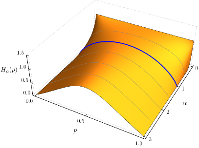
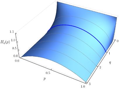
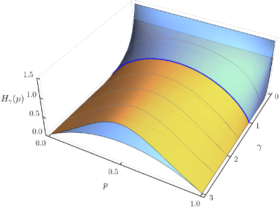
In Fig. 2 we show the behavior of the Rényi entropy (left) and the Tsallis entropy (right) for a Bernoulli random variable which has two possible outcomes, one with probability and the other with probability , as a function of and and and , respectively. We see that the two entropies are maximized at , that is, in the case with the two random variables having equal probabilities. Also, as and approach unity, the two results converge to the Shannon entropy, but when they are different, the two entropies become more and more distinct. In particular, the Rényi entropy is greater or equal to the Tsallis entropy, when , but it is lower or equal to for . We illustrate this in Fig. 3, where we display the results of Fig. 2 for in the same diagram, visually comparing the two entropies explicitly.
We think it is of current interest to examine different quantum graphs, with several arrangements of vertices and edges, to see how the results appear in these new situations. We do this in the next section, but we know that the Rényi and the Tsallis entropies work to highlight different aspects of physical systems, so in the present work, we do not want to compare these two distinct quantifiers against each other. Instead, we concentrate mainly on how the scattering Rényi entropy and the average scattering Rényi entropy behave as one varies the parameter , and how the scattering Tsallis entropy and the average scattering Tsallis entropy change as one modifies the parameter . As one knows, when diminishes towards zero, the Rényi entropy increasingly weighs all events with nonzero probability more equally, regardless of their probabilities. However, when increases towards infinity, it is increasingly determined by the events of the highest probability. For the Tsallis entropy, its nonadditive behavior is highlighted when one considers two independent systems and , with joint probability density obeying : one gets for the entropy that , showing that for and for . These are manifestations to be used to help us to understand the examples investigated below.
3 Examples
Let us now calculate the scattering entropies for different types of graphs [45], when we add only two leads to the graph, as we illustrate in Fig. 1 (middle), and when we add one lead to each vertex of the graph, as we illustrate in Fig. 1 (right). Interesting possibilities refer to the presence of several scattering channels, where the scattering entropies provide a useful simplification in the analysis, condensing the several possible results in just one. There are some limiting cases that can be observed: one is when all scattering channels are equivalents, which corresponds to the case where the scattering has the highest informational value, resulting in the maximum value for the scattering entropies; another is when the scattering has one preferential channel, such that the one scattering coefficient equals unity, leading to vanishing scattering entropies. Below we illustrate several distinct possibilities.
To exemplify the main results of the previous section, let us now focus on some specific cases of quantum graphs. We start with some arrangements of graphs, like the series and the parallel layouts. Then, we examine results for specific types of graphs with vertices and leads, or channels, connected to them. In the last case, the classes of graphs which we will consider are the cycle (), wheel () and the complete () on vertices. In general, we calculate the scattering coefficients of these quantum graphs using the Neumann boundary condition.
3.1 Quantum graphs in series and parallel layouts
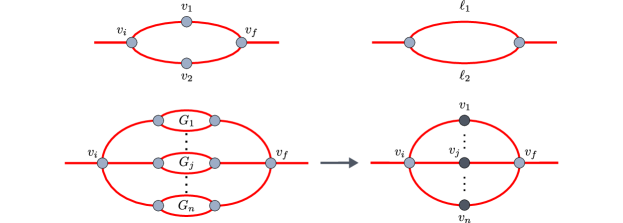
To introduce different arrangements of graphs, we can start with one of the simplest graphs, which is defined by two vertices connected by one edge (a path graph on vertices, ). By adding one lead to each vertex, as shown in Fig. 4 (top), and defining boundary conditions on them, we obtain the reflection {,} and transmission {,} amplitudes associated to the respectively vertices and . Furthermore, the metric in this quantum graph is defined by a length of the edge which connects these vertices.
For notational ease in this subsection, the reflection and transmission amplitudes will be denoted by and instead of . Thus, defining the scattering amplitudes of this quantum graph are [42]
| (13) |
and
| (14) |
where is used to identify that the vertices and are arranged in a series layout.


These equations can be used recursively to obtain the scattering amplitudes when adding one more vertex () in series with the first quantum graph, by defining and . In this sense, it is possible to obtain the scattering amplitudes for the general case of by transforming these equations to a recursive equation system in the form
| (15) | ||||
| (16) |
Here we have a set of vertices in a series layout, , which allow us to study a set of renormalized quantum graphs displayed in Fig. 4 (bottom, right). Thus, with Eqs. (15) and (16), we have an alternative recursive method to the transfer matrix method for quantum graphs [46] arranged in this layout, which only needs the scattering amplitudes of each quantum graph.
Now we can find the scattering amplitudes for the special case where quantum graphs with the same scattering amplitudes of reflection () and transmission () are arranged in a series layout. Thus, the final form of its reflection and transmission amplitudes are
| (17) |
and
| (18) |
with
| (19) |
A second layout can be defined starting with two vertices and in parallel as shown in Fig. 5 (top, left), where both vertices are only connected to the other two vertices and , which are the vertices with leads attached to them. Here we define the vertices and with the same amplitudes and , and and with the respectively scattering amplitudes , and , . Furthermore, to simplify these equations, here we define , where is the distance between the vertices in parallel to the ones with leads attached, as shown in Fig. 5 (top, left). So, we have the reflection and transmission for this system as
| (20) | ||||
| (21) |
where
| (22) |
In order to identify this parallel layout, we now use .
With these equations, we can approach the case where all the vertices have a Neumann boundary condition (, , , ). Letting and , we obtain the equations for the quantum graph in Fig. 5 (top, right), which has scattering amplitudes
| (23) |
and
| (24) |
These equations allow us to study quantum interference due to the difference in the length of its edges. Works that have used these graphs have proposed the use of them in a series layout as quantum devices [44, 47]. Here we use the particular case where both edges have the same length ( and ), which leads to the quantum amplitudes
| (25) |
| (26) |
We can generalize the model of quantum graphs in a parallel layout by defining a set of quantum graphs that are connected only to the same two vertices, as illustrated in the Fig. 5 (bottom, left). As these quantum graphs can be renormalized to vertices, each one having the same scattering amplitudes of the original quantum graph . Here we extend the Eqs. (20) and (21) to the case where we have quantum graphs in this parallel layout. An interesting result considers the model where all the quantum graphs in parallel have the same scattering amplitudes and , and the two lateral vertices have amplitudes and . So, this model leads to scattering amplitudes in the form
| (27) |
and
| (28) |
Finally, setting the Neumann boundary condition in the vertices connected to the leads, here we have the amplitudes and , then the final result is
| (29) |
and
| (30) |
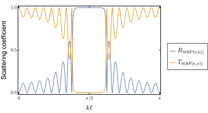
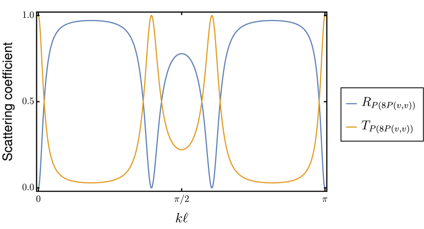
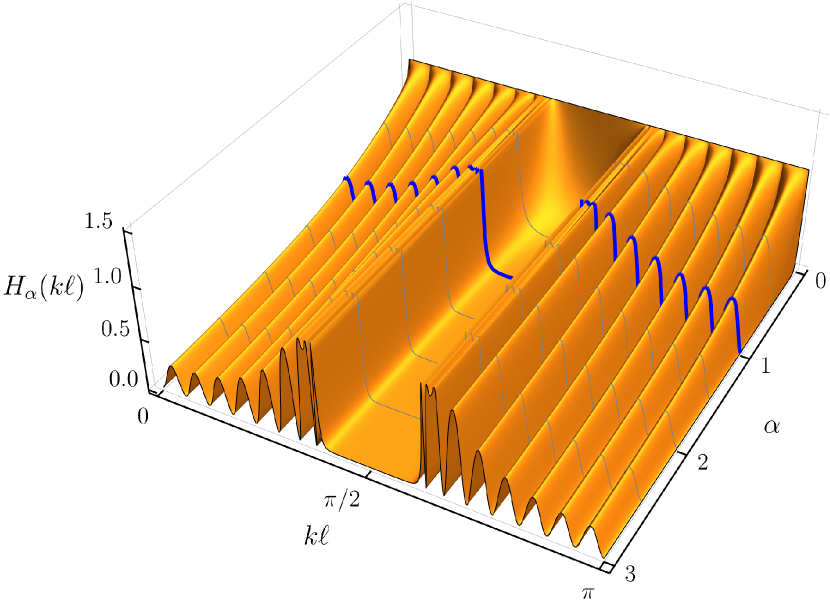
To illustrate how is the behavior of the scattering from the same set of quantum graphs, but organized in different layouts, we considered a set of eight of the same quantum graph showed in Fig. 5 (top, right) with , which has the scattering amplitudes obtained in Eqs. (25) and (26). The series layout for this case is illustrated in Fig. 4 (bottom) and has the scattering amplitudes given in Eqs. (17) and (18), being the reflection and transmission coefficients illustrated in Fig. 6 (left). For the parallel arrangement illustrated in Fig. 5 (bottom, left), we obtained the coefficients from Eqs. (29) and (30), which behaviors are illustrated in Fig. 6 (right). Finally, the scattering entropies to these examples from the Fig. 6 are illustrated in the Fig. 7, for the Rényi (top) and Tsallis (bottom) scattering entropies, for both series (left) and parallel (right) arrangements.
3.2 Cycle quantum graph with leads
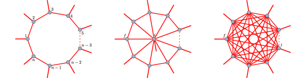
Cycle graphs, , are defined as a set of vertices, each one with degree two, therefore all the vertices have two neighbor vertices. To define the scattering in the cycle quantum graph, we need to define the entrance and the set of exit vertices, which have leads attached to them, thus increasing their degrees by one. In the present case, we define that every vertex in these graphs are connected to one lead, being the vertex labeled as the entrance vertex, and the remaining vertices, labeled from to , are the exit channels; see Fig. 8.
To simplify the final form of equations in this subsection, we define the quantities and in the following form
| (31) |
| (32) |
Thus, for a quantum graph with leads, we can write the reflection amplitude as
| (33) |
For the transmission amplitude, there is a dependence on which one is the exit vertex, so we label the two first neighbors of the entrance vertex () as the vertices and , the two second neighbors as the vertices and , and so on, as shown in Fig. 8 (left). Hence, the transmission amplitudes are defined in terms of the chosen vertex , with . Thus, we have
| (34) |
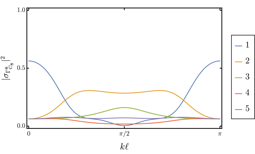
As we considered all the vertices having the same boundary conditions, it leads to a vertex be equivalent to another vertex with for odd , and for even . In this way, the number of scattering channels for an odd number of vertices is reduced by , and the reduction is of for even . So, for such graphs we have scattering amplitudes and due to the symmetry of them, for the odd graphs there are different values of them and for even , the number of different scattering amplitudes is , as we exemplify in the Fig. 9 .
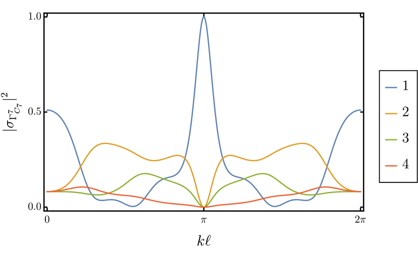
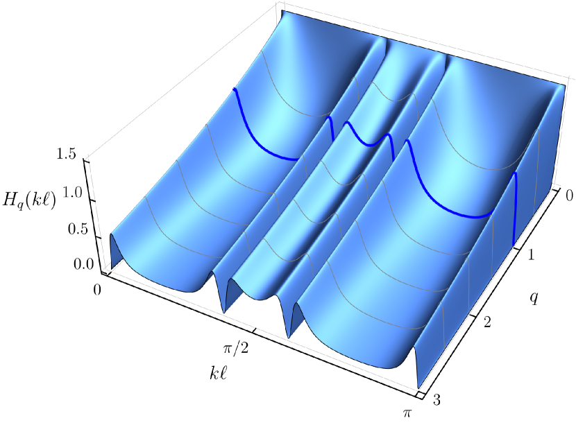
In this sense, considering all the scattering coefficients that we have obtained, we can obtain the scattering entropies which are illustrated in Fig. 10, being the top two for the Rényi scattering entropy and the bottom two for Tsallis scattering entropy. In both cases, we obtained the entropies for and , where we observe that for the cycle quantum graphs with an odd number of vertices, the entropies are zero for the values of , with , the same points where the reflection is maximum and all the other scattering coefficients for any other channel are equal to zero. We notice that the scattering entropies are different, so they can be used to induce distinct results under the same quantum graph type.
3.3 Wheel quantum graphs with leads
The wheel graphs, , are defined as a set of vertices, in which one vertex have degree , which here we call , while all the others have the same degree (), and are labeled as . Thus, to define this quantum graph with channels in the most symmetrical way, we consider the central vertex as the entrance channel, while the others are all exit channels. So, the vertex now has degree , while all other vertices have degree . See Fig. 8 (middle) for an illustration.
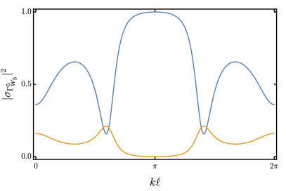
Due to the symmetry and as all the vertices have the same boundary condition, we get the same transmission amplitude for these vertices. Therefore, the expression for the reflection and transmission amplitudes in the wheel quantum graph with Neumann boundary conditions are, respectively,
| (35) |
and
| (36) |
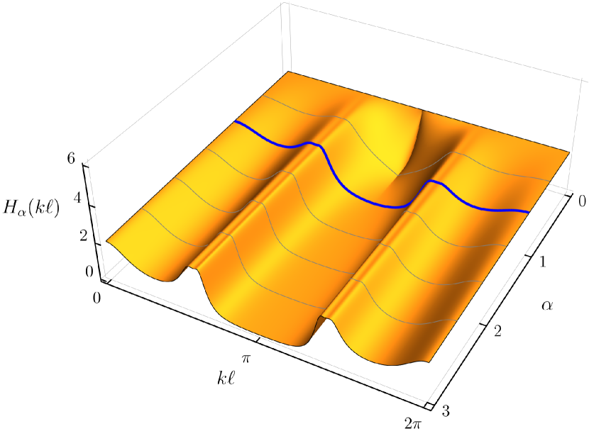
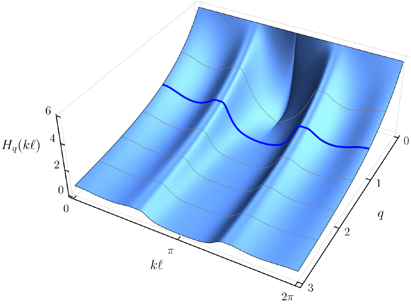
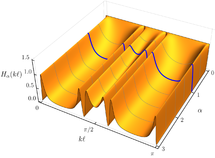
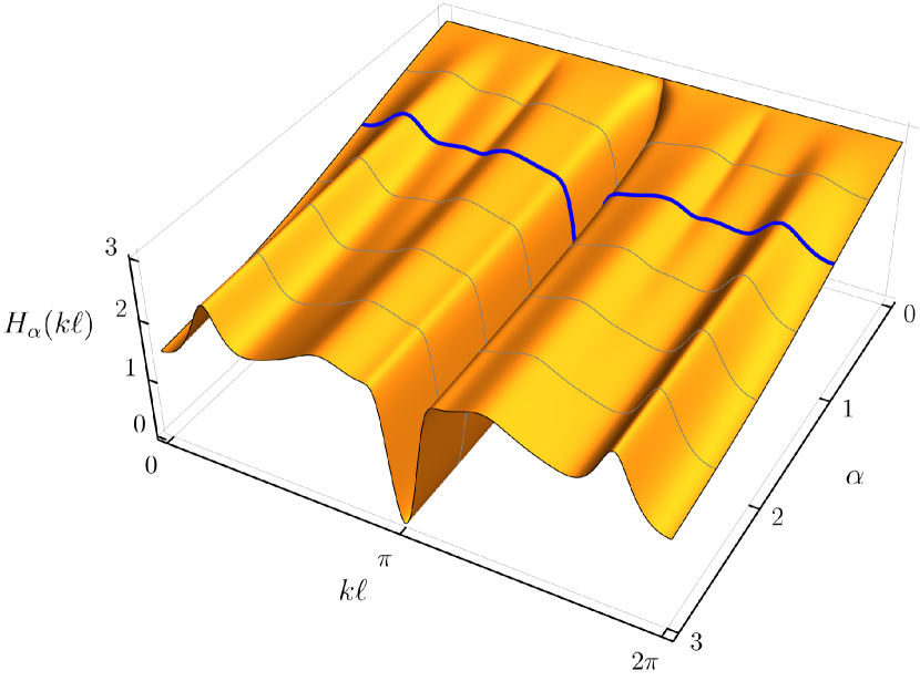
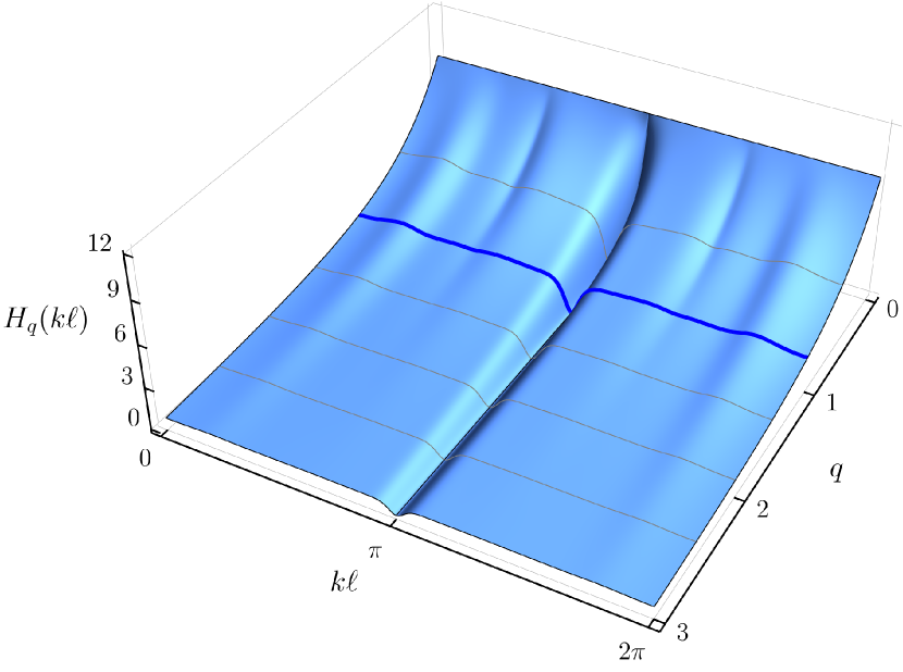
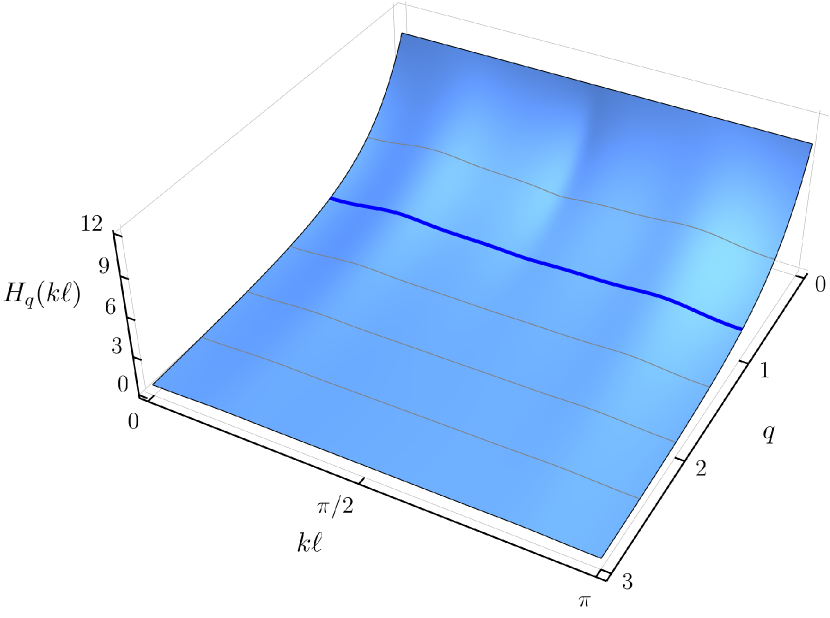
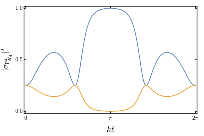
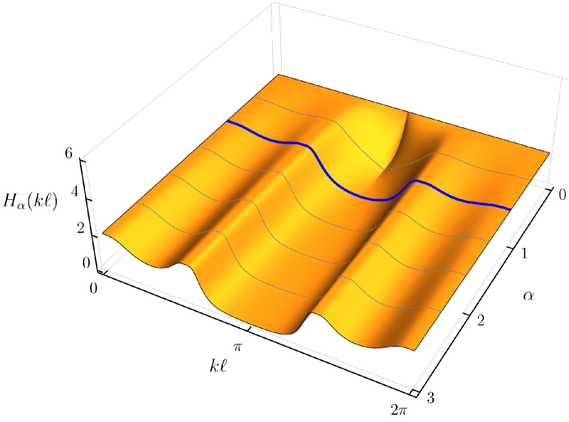
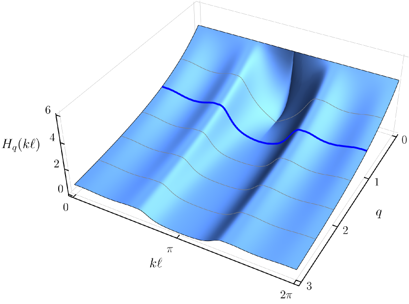
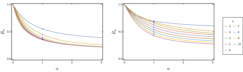
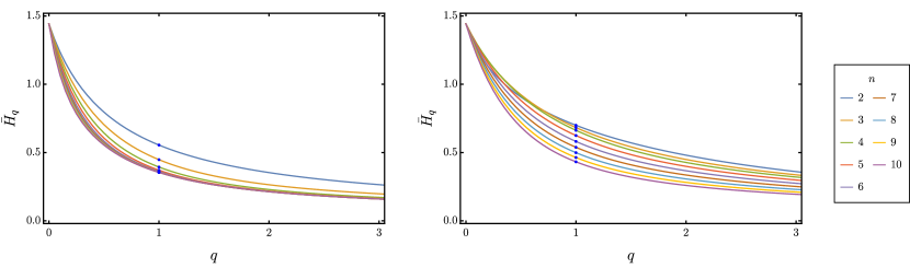
We display the above results for the scattering entropies in Fig. 11, in the case of a wheel quantum graph with vertices. Also, in Fig. 12 we display both the Rényi and Tsallis scattering entropies, highlighting the case of the Shannon entropy in blue for the same wheel graph with vertices. We notice that the scattering entropies are different, so they can be used to induce distinct results under the same quantum graph type.
3.4 Complete quantum graphs with leads
In the complete graphs, , we have a set of vertices, where each one is connected to all other vertices. With the addition of the leads, each vertex has degree . This is illustrated in Fig. 8 (right). In this case, due to the symmetry of these quantum graphs, any lead taken as the entrance we have the same expressions for the scattering amplitudes. With the Neumann boundary conditions in each vertex, we then get the reflection amplitude in the form
| (37) |
and the transmission amplitude as
| (38) |
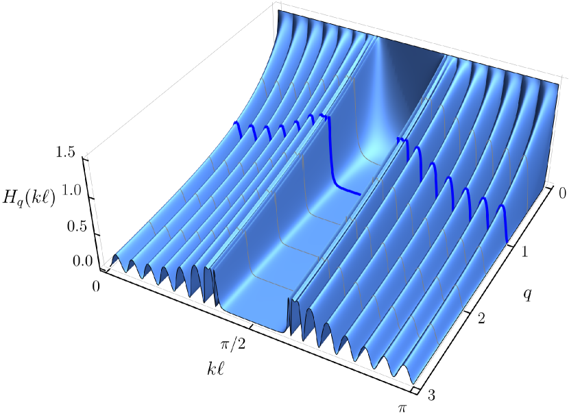
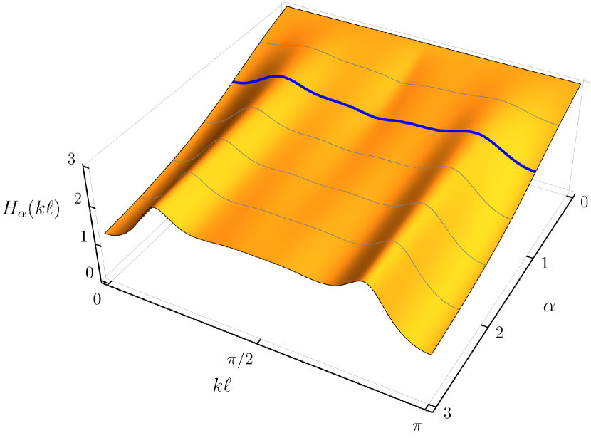
We display the above results for the scattering entropies in Fig. 13, in the case of a complete graph with vertices. Also, in Fig. 14 we display both the Rényi and Tsallis scattering entropies, highlighting the case of the Shannon entropy in blue for the same complete graph with vertices. We notice that the scattering entropies are different, so they can be used to induce distinct results under the same quantum graph type.
3.5 Average scattering entropies
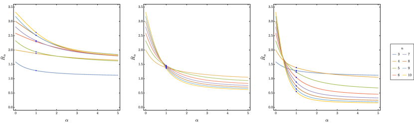
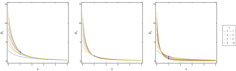
Since all the quantum graphs that we have studied in previous sections have periodic scattering probabilities, we can also study their average scattering entropies, which are given in Eq. (12) on general grounds. We implemented distinct investigations, and in Figs. 15 and 16 we display the results for some series and for parallel arrangements, respectively. The values of the average scattering entropy decrease as one increases the parameter for Rényi and the parameter for Tsallis. Similar results are also depicted in Figs. 17 and 18, for distinct graphs of the cycle, wheel, and complete graphs, respectively. The values of the average scattering Rényi and Tsallis entropies also decrease when one increases and , respectively. The results depicted in Figs. 15, 16, 17 and 18 show the general behavior, that the average entropies always decrease, as one increases the parameters and .
4 Conclusion
In this work, we investigated scattering and entropies entropies in distinct types of quantum graphs. The process of scattering in quantum graphs is developed via Green’s function approach to computing the quantum coefficients in quantum graphs. After describing the procedure on general grounds, we added the scattering entropy and the average scattering entropy using the concept of entropy due to Shannon, and the respective generalizations to the case of Rényi and Tsallis entropies. Since we have already considered the case of Shannon in previous works, the use of the Rényi and Tsallis entropies can be implemented similarly, so they are somehow easy to describe and understand, and can be manipulated to lead us back to the case of the Shannon entropy within trustable mathematical manipulations.
After describing the general results, we implemented specific computations to calculate the scattering Rényi and Tsallis entropies in several distinct situations, described by types of graphs that in general appear in the study of quantum graphs, among them the series and parallel, and the circle, wheel and complete graphs. Since the Rényi and Tsallis entropies depend on distinct real parameters, we developed results with the parameters evaluated within intervals of current interest, including the cases where they reproduce the Shannon entropy. The results show distinct behavior, and the scattering Rényi and Tsallis entropies may induce very different values. This is interesting since the difference can be identified easily. The important distinctions among them, depending on the wave number of the incoming signal may certainly be used in applications, in particular as a filter to block the quantum transport under certain circumstances. The use of quantum graphs as filters was already considered in [48, 47, 49] and we can also think of applying the above results in this line of study.
These general results indicate that for all types of quantum graphs that we studied above, if one thinks of the Rényi entropy as an index of diversity, and the Tsallis entropy as an index of nonadditivity, in the same quantum graph, the index of diversity is higher than or equal to the index of nonadditivity when , but it is lower than or equal to when . For the Tsallis entropy, we know that given two independent systems and , with joint probability density obeying , we have for the entropy that , showing that for and for . For the Rényi entropy, we know that when diminishes towards zero, it increasingly weighs all events with nonzero probability more equally, regardless of their probabilities. However, when increases towards infinity, it is increasingly determined by the events of the highest probability. In this sense, for diminishing towards zero, the Rényi entropy counts an increasing number of accessible states, increasing both the scattering Rényi entropy and the average scattering Rényi entropies. However, for increasing to higher and higher values, the Rényi entropy seems to select the events of higher and higher probabilities, diminishing both the scattering and the average scattering entropies. There are other interesting results: for the Tsallis entropy, in particular, from the average scattering entropy displayed in the center panel in Fig. 18 for the wheel family of quantum graphs, one notices that the average Shannon entropy does not significantly depends on the number of vertices in the quantum graph, but there are significant variation of the results for diminishing towards zero, where the entropy of a joint system seems to be higher than the addition of the entropies of its individual parts.
The above results are of current interest, and they may be used to further study specific systems. In particular, the work [50], established an important connection between quantum graphs and microwave networks, and this may be further investigated to strengthen the results of the present work. For instance, in the recent work [51], the authors described spectral duality in graphs and microwave networks, which can be further considered in the case of the open quantum graphs studied above. This is based on the fact that the connection between quantum graphs and microwave networks work for both spectral and scattering properties. The results of the present work can also be used in several other distinct directions, in particular, in the case of reflection and transmission in ring-like systems with symmetric and asymmetric triple junctions [52] and in applications concerning to the quantum transport in single-molecule junctions, that is, in devices in which a molecule is electrically connected by two electrodes; see, e.g., the recent reviews [53, 54] and references therein. We hope to report on some related specific issues in the near future.
Acknowledgments
This work was partially supported by the Brazilian agencies Conselho Nacional de Desenvolvimento Científico e Tecnológico (CNPq), Instituto Nacional de Ciência e Tecnologia de Informação Quântica (INCT-IQ), and Paraíba State Research Foundation (FAPESQ-PB, Grant 0015/2019). It was also financed by the Coordenação de Aperfeiçoamento de Pessoal de Nível Superior (CAPES, Finance Code 001). FMA and DB also acknowledge financial support by CNPq Grants 314594/2020-5 (FMA) and 303469/2019-6 (DB).
References
- [1] G. Berkolaiko, P. Kuchment, Introduction to Quantum Graphs, American Mathematical Society, 2012.
- [2] C. E. Shannon, A mathematical theory of communication, Bell System Technical Journal 27 (3) (1948) 379–423. doi:10.1002/j.1538-7305.1948.tb01338.x.
-
[3]
A. Rényi, L. Vekerdi,
Probability Theory,
Applied mathematics and mechanics, North-Holland Publishing Company, 1970.
URL https://books.google.com.br/books?id=EraDtAEACAAJ - [4] X. Dong, Shape dependence of holographic Rényi entropy in conformal field theories, Phys. Rev. Lett. 116 (25) (2016) 251602. doi:10.1103/physrevlett.116.251602.
- [5] Z. Gong, L. Piroli, J. I. Cirac, Topological lower bound on quantum chaos by entanglement growth, Phys. Rev. Lett. 126 (16) (2021) 160601. doi:10.1103/physrevlett.126.160601.
- [6] B. Shi, I. H. Kim, Domain wall topological entanglement entropy, Phys. Rev. Lett. 126 (14) (2021) 141602. doi:10.1103/physrevlett.126.141602.
- [7] A. Belin, L.-Y. Hung, A. Maloney, S. Matsuura, R. C. Myers, T. Sierens, Holographic charged Rényi entropies, J. High Energy Phys. 2013 (12) (2013) 59. doi:10.1007/jhep12(2013)059.
- [8] P. Bueno, P. A. Cano, Á. Murcia, A. R. Sánchez, Universal feature of charged entanglement entropy, Phys. Rev. Lett. 129 (2) (2022) 021601. doi:10.1103/physrevlett.129.021601.
- [9] C. Tsallis, Possible generalization of Boltzmann-Gibbs statistics, J. Stat .Phys. 52 (1-2) (1988) 479–487. doi:10.1007/bf01016429.
- [10] C. Tsallis, Introduction to Nonextensive Statistical Mechanics, Springer New York, 2009. doi:10.1007/978-0-387-85359-8.
- [11] C.-Y. Wong, G. Wilk, L. J. L. Cirto, C. Tsallis, From qcd-based hard-scattering to nonextensive statistical mechanical descriptions of transverse momentum spectra in high-energy and collisions, Phys. Rev. D 91 (2015) 114027. doi:10.1103/PhysRevD.91.114027.
- [12] S. Nojiri, S. D. Odintsov, V. Faraoni, Area-law versus Rényi and Tsallis black hole entropies, Phys. Rev. D 104 (8) (2021) 084030. doi:10.1103/physrevd.104.084030.
- [13] G. Sarwar, M. Hasanujjaman, T. Bhattacharyya, M. Rahaman, A. Bhattacharyya, J. e Alam, Nonlinear waves in a hot, viscous and non-extensive quark-gluon plasma, Eur. Phys. J. C 82 (3) (2022) 189. doi:10.1140/epjc/s10052-022-10122-5.
- [14] A. A. Silva, F. M. Andrade, D. Bazeia, Average scattering entropy of quantum graphs, Phys. Rev. A 103 (6) (2021) 062208. doi:10.1103/physreva.103.062208.
- [15] A. A. Silva, F. M. Andrade, D. Bazeia, Average scattering entropy for periodic, aperiodic and random distribution of vertices in simple quantum graphs, Phys. E 141 (2022) 115217. doi:10.1016/j.physe.2022.115217.
- [16] D. Mandal, H. T. Quan, C. Jarzynski, Maxwell’s refrigerator: An exactly solvable model, Phys. Rev. Lett. 111 (3) (2013) 030602. doi:10.1103/physrevlett.111.030602.
- [17] J. M. R. Parrondo, J. M. Horowitz, T. Sagawa, Thermodynamics of information, Nat. Phys. 11 (2) (2015) 131–139. doi:10.1038/nphys3230.
- [18] M. Gleiser, N. Stamatopoulos, Entropic measure for localized energy configurations: Kinks, bounces, and bubbles, Phys. Lett. B 713 (3) (2012) 304–307. doi:10.1016/j.physletb.2012.05.064.
- [19] M. Gleiser, N. Stamatopoulos, Information content of spontaneous symmetry breaking, Phys. Rev. D 86 (2012) 045004. doi:10.1103/PhysRevD.86.045004.
- [20] A. E. Bernardini, N. R. Braga, R. da Rocha, Configurational entropy of glueball states, Phys. Lett. B 765 (2017) 81–85. doi:10.1016/j.physletb.2016.12.007.
- [21] N. R. Braga, R. da Rocha, AdS/QCD duality and the quarkonia holographic information entropy, Phys. Lett. B 776 (2018) 78–83. doi:10.1016/j.physletb.2017.11.034.
- [22] D. Bazeia, D. Moreira, E. Rodrigues, Configurational entropy for skyrmion-like magnetic structures, J. Magn. Magn. Mater. 475 (2019) 734–740. doi:10.1016/j.jmmm.2018.12.033.
- [23] D. Bazeia, E. Rodrigues, Configurational entropy of skyrmions and half-skyrmions in planar magnetic elements, Phys. Lett. A 392 (2021) 127170. doi:10.1016/j.physleta.2021.127170.
- [24] N. R. Braga, O. C. Junqueira, Configuration entropy in the soft wall AdS/QCD model and the wien law, Phys. Lett. B 820 (2021) 136485. doi:10.1016/j.physletb.2021.136485.
- [25] R. da Rocha, Information entropy in AdS/QCD: Mass spectroscopy of isovector mesons, Phys. Rev. D 103 (10) (2021) 106027. doi:10.1103/physrevd.103.106027.
- [26] M. Rigobello, S. Notarnicola, G. Magnifico, S. Montangero, Entanglement generation in QED scattering processes, Phys. Rev. D 104 (11) (2022) 114501. doi:10.1103/physrevd.104.114501.
- [27] G. Karapetyan, Nuclear configurational entropy and high-energy hadron-hadron scattering reactions, Eur. Phys. J. Plus 137 (5) (2022) 590. doi:10.1140/epjp/s13360-022-02736-1.
- [28] G. Karapetyan, R. da Rocha, Nuclear information entropy, gravitational form factor, and glueballs in AdS/QCD, Eur. Phys. J. Plus 137 (7) (2022) 762. doi:10.1140/epjp/s13360-022-02952-9.
- [29] W. Barreto, R. da Rocha, Differential configurational entropy and the gravitational collapse of a kink, Phys. Rev. D 105 (2022) 064049. doi:10.1103/PhysRevD.105.064049.
- [30] W. Barreto, A. Herrera-Aguilar, R. da Rocha, Configurational entropy of generalized sine-Gordon-type models, arXivdoi:10.48550/arXiv.2207.06367.
- [31] T. Kottos, U. Smilansky, Quantum chaos on graphs, Phys. Rev. Lett. 79 (1997) 4794. doi:10.1103/PhysRevLett.79.4794.
- [32] T. Kottos, U. Smilansky, Periodic orbit theory and spectral statistics for quantum graphs, Ann. Phys. (NY) 274 (1999) 76. doi:10.1006/aphy.1999.5904.
- [33] R. Blümel, Y. Dabaghian, R. V. Jensen, Explicitly solvable cases of one-dimensional quantum chaos, Phys. Rev. Lett. 88 (4) (2002) 044101. doi:10.1103/physrevlett.88.044101.
- [34] R. Blümel, Y. Dabaghian, R. V. Jensen, Exact, convergent periodic-orbit expansions of individual energy eigenvalues of regular quantum graphs, Phys. Rev. E 65 (4) (2002) 046222. doi:10.1103/PhysRevE.65.046222.
- [35] T. Kottos, H. Schanz, Quantum graphs: a model for quantum chaos, Physica E 9 (3) (2001) 523. doi:10.1016/S1386-9477(00)00257-5.
- [36] L. Kaplan, Eigenstate structure in graphs and disordered lattices, Phys. Rev. E 64 (3) (2001) 036225. doi:10.1103/PhysRevE.64.036225.
- [37] D. M. Mateos, F. Morana, H. Aimar, A graph complexity measure based on the spectral analysis of the laplace operator, Chaos Solitons Fractals 156 (2022) 111817. doi:10.1016/j.chaos.2022.111817.
- [38] J. Kempe, Quantum random walks: an introductory overview, Contemp. Phys. 44 (2003) 307. doi:10.1080/00107151031000110776.
- [39] G. K. Tanner, From quantum graphs to quantum random walks, in: Non-Linear Dynamics and Fundamental Interactions, Vol. 213, Springer-Verlag, 2006, Ch. From quantum graphs to quantum random walks, pp. 69–87. doi:10.1007/1-4020-3949-2_6.
- [40] F. Diaz-Diaz, E. Estrada, Time and space generalized diffusion equation on graph/networks, Chaos Solitons Fractals 156 (2022) 111791. doi:10.1016/j.chaos.2022.111791.
- [41] F. M. Andrade, S. Severini, Unitary equivalence between the Green's function and Schrödinger approaches for quantum graphs, Phys. Rev. A 98 (6) (2018) 062107. doi:10.1103/physreva.98.062107.
- [42] F. M. Andrade, A. G. M. Schmidt, E. Vicentini, B. K. Cheng, M. G. E. da Luz, Green’s function approach for quantum graphs: an overview, Phys. Rep. 647 (2016) 1–46. doi:10.1016/j.physrep.2016.07.001.
- [43] A. Drinko, F. M. Andrade, D. Bazeia, Narrow peaks of full transmission in simple quantum graphs, Phys. Rev. A 100 (6) (2019) 062117. doi:10.1103/physreva.100.062117.
- [44] A. Drinko, F. M. Andrade, D. Bazeia, Simple quantum graphs proposal for quantum devices, Eur. Phys. J. Plus 135 (6) (2020) 451. doi:10.1140/epjp/s13360-020-00459-9.
-
[45]
R. Diestel, Graph
Theory, 4th Edition, Graduate Texts in Mathematics Vol. 173, Springer, 2010.
URL http://books.google.com.mt/books?id=NvRXJSl9hUUC - [46] G. Tanner, Spectral statistics for unitary transfer matrices of binary graphs, J. Phys. A 33 (18) (2000) 3567. doi:10.1088/0305-4470/33/18/304.
- [47] M. Ahmed, G. Gradoni, S. Creagh, G. Tanner, Meta-networks: Reconfigurable cable network topologies for interference control, in: 2021 IEEE International Joint EMC/SI/PI and EMC Europe Symposium, 2021, pp. 520–523. doi:10.1109/EMC/SI/PI/EMCEurope52599.2021.9559287.
- [48] T. Cheon, P. Exner, O. Turek, Spectral filtering in quantum y-junction, J. Phys. Soc. Jpn 78 (12) (2009) 124004. doi:10.1143/JPSJ.78.124004.
- [49] O. Turek, T. Cheon, Potential-controlled filtering in quantum star graphs, Ann. Phys. (N. Y.) 330 (2013) 104–141. doi:10.1016/j.aop.2012.11.011.
- [50] O. Hul, S. Bauch, P. Pakoński, N. Savytskyy, K. Życzkowski, L. Sirko, Experimental simulation of quantum graphs by microwave networks, Phys. Rev. E 69 (5) (2004) 056205–. doi:10.1103/PhysRevE.69.056205.
- [51] T. Hofmann, J. Lu, U. Kuhl, H.-J. Stöckmann, Spectral duality in graphs and microwave networks, Phys. Rev. E 104 (2021) 045211. doi:10.1103/PhysRevE.104.045211.
- [52] Y. Fujimoto, K. Konno, T. Nagasawa, R. Takahashi, Quantum Reflection and Transmission in Ring Systems with Double Y-Junctions: Occurrence of Perfect Reflection, J. Phys. A 53 (15) (2020) 155302. doi:10.1088/1751-8121/ab7601.
- [53] N. Xin, J. Guan, C. Zhou, X. Chen, C. Gu, Y. Li, M. A. Ratner, A. Nitzan, J. F. Stoddart, X. Guo, Concepts in the design and engineering of single-molecule electronic devices, Nat. Rev. Phys. 1 (3) (2019) 211–230. doi:10.1038/s42254-019-0022-x.
- [54] P. Gehring, J. M. Thijssen, H. S. J. van der Zant, Single-molecule quantum-transport phenomena in break junctions, Nat. Rev. Phys. 1 (6) (2019) 381. doi:10.1038/s42254-019-0055-1.