A closure for the Master Equation starting from the Dynamic Cavity Method

Abstract

We consider classical spin systems evolving in continuous time with interactions given by a locally tree-like graph. Several approximate analysis methods have earlier been reported based on the idea of Belief Propagation / cavity method. We introduce a new such method which can be derived in a more systematic manner, and which performs better on several important classes of problems.

1 Introduction

Problems across many scientific disciplines require understanding the non-equilibrium dynamics of many interacting variables. The variables could be spins in condensed-matter physics[1], cells or reactions in biology [2], neurons in neurosciences and machine learning [3], etc. In all these cases the mathematical formulation is almost always the same. Given $N$ variables $\underline{\sigma}=\{\sigma_{1},\cdots,\sigma_{N}\}$ one needs, in principle, to solve the master equation:

$$\frac{dP(\underline{\sigma})}{dt}=-\sum_{i=1}^{N}[r_{i}(\underline{\sigma}\rightarrow\underline{\sigma^{\prime}})P(\underline{\sigma})-r_{i}(\underline{\sigma^{\prime}}\rightarrow\underline{\sigma})P(\underline{\sigma^{\prime}})]$$ (1)

where $P(\underline{\sigma})$ is the probability of the configuration $\underline{\sigma}$ and $r_{i}(\underline{\sigma^{\prime}}\rightarrow\underline{\sigma})$ defines the transition rates from configuration $\underline{\sigma^{\prime}}$ to $\underline{\sigma}$.

Equation (1) is a Markovian first order differential equation. Although it is compact and formally simple, it implies the tracking in time the probabilities of $2^{N}$ discrete states, a daunting task that can be done only for very small systems. A large amount of work has therefore been devoted to find approximate solutions or closure schemes able to provide an accurate yet computationally manageable description of this dynamics.

The transition rate $r_{i}$ of spin $i$ can in principle depend only on spin $i$ itself, on all the spins, or on spin $i$ and some set of neighbours $\partial i$. In the last case, which is the one considered here, the dependency sets of all the spins and how they are connected define a directed graph. In this graph there is a link $j\to i$ if and only if $j\in\partial i$; the dependency of $r_{i}$ of spin $i$ (if present) has to be taken into account separately. It is straightforward to show that the probability of variable $\sigma_{i}$ only changes as

$$\frac{dP(\sigma_{i})}{dt}=-\sum_{i=1}^{N}[r_{i}(\sigma_{i},\sigma_{\partial i})P(\sigma_{i},\sigma_{\partial i})-r_{i}(-\sigma_{i},\sigma_{\partial i})P(-\sigma_{i},\sigma_{\partial i})]$$ (2)

Although apparently simpler than (1), equation (2) is not closed, to compute $P(\sigma_{i})$ on the LHS one needs information about $P(\sigma_{i},\sigma_{\partial i})$. The problem then reduces to find a proper closure scheme for equation (2). The main goal of this work is to propose and test a new such scheme.

In parallel to (1) and (2) one can also consider the analogous equations for discrete time. One example would be a time-discretization of (1) and (2) with a finite time step $\Delta t$. The discrete time model allows also for other types of dynamics, but is nevertheless in a mathematical sense simpler. The history of a discrete-time variable over a finite time interval is a finite-dimensional variable, while the history of a continuous-time variable is infinite-dimensional. Many techniques introduced for discrete time further have only a trivial limit as $\Delta t$ tends to zero. In short, the continuous-time case is what is directly appropriate for most applications, and also needs additional treatment compared to the discrete case. The work reported in this paper is another effort in this direction.

The paper is organized as follows. In section 2 we review the Dynamic cavity method in the version introduced for discrete-time in [4]. In Section 3 we introduce our new closure scheme for the continuous-time case. Then, Section 4 shows the comparison of our solution with Monte Carlo simulations and with alternative closure schemes build on similar principles. Finally we present the conclusions of our work, they also summarize the main limitations of our approach and highlight possible paths for future developments.

2 Dynamic cavity method

2.1 Definition, specificity and main problem

The standard cavity method is a means to compute marginals of a Gibbs-Boltzmann distribution by exchanging messages [5]. When it converges the cavity method is computationally efficient requiring a number of operations polynomial in system size. The cavity method is exact when the interaction graph is a tree and asymptotically exact for many types of a locally tree-like interaction graphs. As in this Letter we consider statistical inference we will not discuss the use of dynamic cavity to retrodict the origin of epidemics and similar processes, for this see [6] and [7]. To stay inside the sphere of physical problems we will also not consider the recent use of dynamic cavity to model and predict the evolution of an epidemic [8, 9].

We will consider a dynamics specified by an graph of the same locally tree-like type. Let the history of variable $i$ up to time $t$ be $X^{t}_{i}$, and let the value of variable $i$ at time $t$ be $\sigma_{i}(t)$. For an Ising variable we can formally define $X^{t}_{i}=(\sigma_{i}(t_{0}),n,t_{1},t_{2},\ldots)$ where $\sigma_{i}(t_{0})$ is the initial value of the spin, $n$ is the number of jumps in the time interval $[t_{0}:t]$ and $t_{1},t_{2},\ldots$ are the set of spin flip times.

We will consider the setting where the one-time joint probability of all the variables satisfies a high-dimensional differential equation (Master equation) of the type

$$\frac{d}{dt}P\left(\sigma_{1},\ldots,\sigma_{N},t\right)=\sum_{\sigma^{\prime}_{1},\ldots,\sigma^{\prime}_{N}}\Gamma_{\mathbf{\sigma},\mathbf{\sigma}^{\prime}}P\left(\sigma^{\prime}_{1},\ldots,\sigma^{\prime}_{N},t\right).$$ (3)

The main idea is now to trade the high-dimensional probability $P\left(\sigma_{1},\ldots,\sigma_{N},t\right)$ with the infinite-dimensional probability $P(X^{t}_{i})$. In so doing the goal is to arrive at an accurate and computationally effective description of the one-time marginal probabilities $P_{i}\left(\sigma_{i},t\right)$. To proceed we first note that the locally tree-like interaction graph describes the transition matrices $\Gamma_{\mathbf{\sigma},\mathbf{\sigma}^{\prime}}$ which satisfy $\sum_{\mathbf{\sigma}}\Gamma_{\mathbf{\sigma},\mathbf{\sigma}^{\prime}}=1$ for every value of $\mathbf{\sigma}^{\prime}$. The joint probability over the histories of all the variables can then, up to technicalities, be written

$$P^{t}(X^{t}_{1},\ldots,X^{t}_{N})=\Gamma_{\mathbf{\sigma}(t),\mathbf{\sigma}(t-\epsilon)}\cdots\Gamma_{\mathbf{\sigma}(t_{0}+\epsilon),\mathbf{\sigma}(t_{0})}\cdot P^{0}(\sigma_{1},\ldots,\sigma_{N},t_{0}).$$ (4)

We either assume that the initial probability distribution $P^{0}$ is so far in the past that it does not matter, or that it only has the same dependencies as in $\Gamma$. For instance, it can be factorized.

It follows from the Markovian nature of the Master equation (3) that the probabilities of different variables to flip in a short time interval $\Delta t=\epsilon$ are independent. This is in any case natural in the continuous-time limit where these probabilities are given by $\Delta t\cdot r_{i}$ where $r_{i}$ is the instantaneous flip rate of spin $i$. For the Ising ferromagnet with Glauber dynamics, which we show as a numerical example in Fig. 1, the rates are

$$r_{i}(\sigma_{i},\sigma_{\partial i})=\alpha\frac{e^{-\frac{J}{k_{B}T}\sum_{j\in\partial i}\sigma_{i}\sigma_{j}}}{\sum_{s}e^{-\frac{J}{k_{B}T}\sum_{j\in\partial i}s\,\sigma_{j}}},$$ (5)

where $\alpha$ is a constant of dimension inverse time and $J$ is the pairwise interaction energy.

The dependencies in the joint probability distribution (4) includes effects of the type that if $k$ and $j$ are both in the neighborhood of $i$ as given by the energy function, they are also related by the denominator in the expression for the rate $r_{i}$. The total statistical dependencies in (4) therefore include many local loops. A systematic approach to resolve these loops is by graph expansion [10, 4]. This approach associates a pair of variables $(X^{t}_{i},X^{t}_{j})$ to each link $(ij)$ in the original dependency graph and imposes hard constraints $C_{i}$ that all variables of the type $X^{t}_{i}$ in all links $(ij)$ take the same value. The probability distribution (4) can then equivalently be written

$$P^{t}\big{(}\{X^{t,(ij)}_{i},X^{t,(ij)}_{j}\}\big{)}=\prod_{i}\Phi_{i}\big{(}X^{t}_{i},\{X^{t,(ij)}_{j}\}_{j\in\partial i}\big{)}\prod_{i}C_{i}$$ (6)

where the local loops have been resolved. The first argument $X^{t}_{i}$ on the right hand of above can be any of the $X^{t,(ij)}_{i}$ as by the constraint $C_{i}$ they are all the same. Using the theory of Random Point Processes [11] the local weight functionals can further be written

$$\Phi_{i}\left(X^{t}_{i},X^{t}_{\partial i}\right) = \prod_{s=1}^{n}r_{i}\left(\sigma_{i}(t_{s}),\sigma_{\partial i}(t_{s})\right)\cdot e^{-\int_{t_{0}}^{t_{1}}r_{i}\left(\sigma_{i}(\tau),\sigma_{\partial i}(\tau)\right)\,d\tau}$$ (7)

$$\qquad\cdot\prod_{s=1}^{n}e^{-\int_{t_{s}}^{t_{s+1}}r_{i}\left(\sigma_{i}(\tau),\sigma_{\partial i}(\tau)\right)\,d\tau}$$

where we recall that $X^{t}_{i}$ is defined by $n$, the number of jumps of spin $i$ in a time interval $[t_{0},t_{f}]$, the initial spin state, and the jump times. For given $n$ the last time ($t_{n+1}$) in above is $t_{f}$.

After applying the graph expansion the right-hand side of (6) is like a Boltzmann weight in the standard cavity method with hard constraints, though over an infinite-dimensional space. The marginal probability over one history In the original formulation (4) is defined as $P^{t}_{i}(X^{t}_{i})=\sum_{\mathbf{X}_{\setminus i}}P^{t}(X^{t}_{1},\ldots,X^{t}_{N})$ and in the expanded graph we can first marginalize to the joint probability of the set $\{X^{t,(ij)}_{i},X^{t,(ij)}_{j}\}_{j\in\partial i}$, where all the $X^{t,(ij)}_{i}$ are the same due to the constraint $C_{i}$, and then marginalize separately over the $X^{t,(ij)}_{j}$. The cavity (or Belief Propagation) output equation is then

$$P^{t}_{i}(X^{t}_{i})=\sum_{X_{\partial i}^{t}}\Phi_{i}\left(X^{t}_{i},X^{t}_{\partial i}\right)\,\prod_{j\in\partial i}\mu^{t}_{j\to(ji)}(X^{t}_{j},X^{t}_{i}).$$ (8)

In above $\mu^{t}_{j\to(ji)}(X^{t}_{j},X^{t}_{i})$ (a message with two arguments) follows from the graph expansion, and the egress node notation $(ji)$ indicates that these messages are actually passed around in the expanded graph. The cavity (or BP) update equation is on the same level of abstraction

$$\mu^{t}_{j\to(ji)}(X^{t}_{j},X^{t}_{i})=\sum_{X^{t}_{\partial j\setminus i}}\Phi_{j}\left(X^{t}_{j},X^{t}_{\partial j}\right)\prod_{k\in\partial j\setminus i}\mu_{k\to(kj)}(X^{t}_{k},X^{t}_{j}).$$ (9)

Equations (8) and (9) cannot be used as is since the the argument is infinite-dimensional. The equations need to be closed in a suitable finite-dimensional subspace. Furthermore, for the cavity method to be computationally attractive, the subspace should have only one or at most a few spin degrees of freedom per node.

3 Closure scheme

After deriving (9), the next step is to find a convenient parametrization for the histories. We will first briefly review the discrete-time setting, where a simple parametrization is to consider the values of the spins at different times. Each $X_{i}^{t}$ is then approximated by the values of the spins at different times, $X_{i}^{t}\approx(\sigma^{t},\sigma^{t-\epsilon},\cdots,\sigma^{0})$. To arrive at finite-dimensional messages one can then consider a closure on the last $n$ times, which means to take into account a memory of length $n\delta t$. This was the approach (for $n=2$) followed in [4, 12] when studying of the kinetic Ising model under synchronous update dynamics. A more advanced approach based on the matrix product expansion from quantum condensed matter theory was investigated in [13]. Neither of these approaches extend to continuous time.

In a series of papers reviewed in [14] a continuous-time closure was introduced leading to a cavity master equation. Apart from the kinetic Ising model (pair-wise interactions) this versatile approach has also been applied with good results to the ferromagnetic $p$-spin model under Glauber dynamics [15], and to the dynamics of a focused search algorithm to solve the random 3-SAT problem in a random graph [16]. The method has also generalized to provide master equations for the probability densities of any group of connected variables [9]. We will see that the systematic approach introduced here will lead to additional terms, rendering the final formulae somewhat more symmetric and transparent.

In our new approach the starting point is the final-time cavity marginalizations

$$p_{i\to(ji)}\left(\sigma_{i},\sigma_{j}\right)=\sum_{X^{t}_{i}:\sigma_{i}(t)=\sigma_{i}}\sum_{X^{t}_{j}:\sigma_{j}(t)=\sigma_{j}}\mu_{i\to(ji)}\left(X^{t}_{i},X^{t}_{j}\right)$$ (10)

This is different from the earlier approach reviewed in [14] where the starting point was the single-site marginals $p_{i}\left(\sigma_{i}\right)$. The closure of the cavity update equations as master-equation-like differential equations reads

$$\frac{d}{dt}{p}_{i\to(ij)}(\sigma_{i},\sigma_{j})=\sum_{\sigma_{\partial i\setminus j}}\Big{[}r_{i}(\sigma_{i},\sigma_{\partial i})\prod_{k\in\partial i\setminus j}p_{k\to(ki)}(\sigma_{k}\mid\sigma_{i})p_{i\to(ij)}(\sigma_{i},\sigma_{j})$$

$$\qquad-r_{i}(-\sigma_{i},\sigma_{\partial i})\prod_{k\in\partial i\setminus j}p_{k\to(ki)}(\sigma_{k}\mid-\sigma_{i})p_{i\to(ij)}(-\sigma_{i},\sigma_{j})\Big{]}$$

$$\qquad-r_{j}(\sigma_{j},\sigma_{i})p_{i\to(ij)}(\sigma_{i},\sigma_{j})+r_{j}(-\sigma_{j},\sigma_{j})p_{i\to(ij)}(\sigma_{i},-\sigma_{j}).$$ (11)

In the above the conditional probabilities in the cavity are defined as: $p_{i\to(ij)}(\sigma_{i}\mid\sigma_{j})=\frac{p_{i\to(ij)}(\sigma_{i},\sigma_{j})}{\sum_{s}p_{i\to(ij)}(s,\sigma_{j})}$

Further, $r_{i}(\sigma_{i},\sigma_{\partial i})$ and $r_{j}(\sigma_{j},\sigma_{i})$ are the defined jump rates of spins $i$ and $j$ in the cavity graph obtained by eliminating all neighbours of $j$ except $i$. The rate $r_{i}$ hence depends on all neighbours of $i$ in the original graph, including $j$, while the rate $r_{j}$ only depends on $i$ and $j$.

The fundamental object of the cavity output equations are analogously the final-time marginalizations $P_{i}\left(\sigma_{i}\right)=\sum_{X^{t}_{i}:\sigma_{i}(t)=\sigma_{i}}P^{t}_{i}(X^{t}_{i})$ and the differential equations substituting for (8) are

$$\frac{d}{dt}{P}_{i}(\sigma_{i}) =\sum_{\sigma_{\partial i}}\Big{[}r_{i}(\sigma_{i},\sigma_{\partial i})\prod_{k\in\partial i\setminus j}p_{k\to(ki)}(\sigma_{k}|\sigma_{i})P_{i}(\sigma_{i})$$ (12)

$$\quad-r_{i}(-\sigma_{i},\sigma_{\partial i})\prod_{k\in\partial i\setminus j}p_{k\to(ki)}(\sigma_{k}|-\sigma_{i})P_{i}(-\sigma_{i})\Big{]}.$$

In summary, we claim that the combination of equations (11) and (12) constitutes a proper closure scheme that should approximately describe the dynamics of the Master equation (1) for continuous time and discrete variables.In the next section we will see how this expectation fares in numerical tests.

4 Numerical illustrations

In Fig. 1 we show numerical results on the kinetic Ising model obtained using (11) and (12); it can be checked that they improve on the earlier version of the continuous-time closure [17]. The left panel (Fig. 1a) contains results for the one-dimensional Ising ferromagnet, the exact solution of which was obtained by Glauber [18] is represented with lines and points. In this simple model, the first version of the cavity closure is surprisingly far from the solution, while the new closure presented here gives considerably better results.

On the other hand, Fig. 1b shows results on the Ising ferromagnet defined over an Erdos-Renyi graph. Both the original and the new closure give results that are very similar to the dynamics of the Monte Carlo simulations. Nevertheless, it is possible to appreciate a small improvement of the accuracy provided by the new approach. The local errors in the inserted graphic point to the same conclusion for all temperatures.

(a)

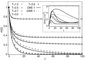
(b)

Figure 1: Continuous-time dynamics of the Ising ferromagnet. Both panels compare the results of the earlier cavity closure [17] (thick continuous lines) and the new closure (dashed lines). In all calculations, an initially fully magnetized system evolves in time in contact with a heat bath at a given temperature. a) Magnetization of the one-dimensional Ising ferromagnet. Lines with points represent the exact Glauber’s solution for the average magnetization [18]. b) Magnetization in a single instance of an Erdos-Renyi graph with size $N=5000$ and average connectivity $c=3$. The main panel shows the time evolution of the system magnetization. Points are the averages of $s=10,000$ kinetic Monte Carlo simulations of the dynamics. The inserted graphic shows the mean square error $\delta m(t)=(N^{-1}\sum_{i=1}^{N}(m_{i}^{DCAV}(t)-m_{i}^{MC}(t))^{2})^{1/2}$ on scale of order $10^{-2}$.

So far, the integration of equations (11) and (12) outperforms the previous cavity theory, at least on these ferromagnetic systems. However, this is not necessarily true for all models. Let us take, for example, a case with a richer phenomenology, including an spin-glass phase for low temperatures. For this, we explored the Viana-Bray spin-glass model at low temperatures. As can be seen in Fig. 2 it is not so clear which cavity approach is better.

The main panel of Fig. 2a shows the time evolution of the average magnetization. For a very low temperature ($T=0.25$ in the figure), all cavity theories are far from the Monte Carlo results, with no evident winner. The inserted graphic, on the other hand, gives smaller local errors $\delta m(t)=(N^{-1}\sum_{i=1}^{N}(m_{i}^{DCAV}(t)-m_{i}^{MC}(t))^{2})^{1/2}$ for the new theory at the same low temperature. However, the time dependence of the average energy density is less trivial. Apparently, at low temperatures the new cavity method provides a much worse description than the equations derived in [17] (see Fig. 2b). However, notice that, for the same temperatures the local error $\delta e(t)=(N^{-1}c^{-1}\sum_{i\neq j}(e_{ij}^{DCAV}(t)-e_{ij}^{MC}(t))^{2})^{1/2}$ is smaller with the new approach. Finally, in Fig. 2c we show that the time evolution of the Edwards-Anderson parameter $q_{EA}$ is more precisely predicted by the new equations.

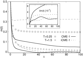
(a)

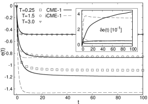
(b)

(c)

Figure 2: Continuous-time dynamics of Viana-Bray spin-glass model defined on a single instance of an Erdos-Renyi graph with $N=1000$ and average connectivity $c=3$. All panels compare the results of the earlier cavity closure [17] (thick continuous lines) and the new closure (dashed lines). As a reference, the results of Monte Carlo simulations of the dynamics are represented with points. In all calculations, an initially fully magnetized system evolves in time in contact with a heat bath at a given temperature. Points are the average of $s=10,000$ Monte Carlo trajectories. a) Magnetization vs. time. The inserted graphic shows the mean square error $\delta m(t)=(N^{-1}\sum_{i=1}^{N}(m_{i}^{DCAV}(t)-m_{i}^{MC}(t))^{2})^{1/2}$ on scale of order $10^{-1}$. b) Energy density vs. time. The inserted graphic shows the mean square error $\delta e(t)=(N^{-1}c^{-1}\sum_{i\neq j}(e_{ij}^{DCAV}(t)-e_{ij}^{MC}(t))^{2})^{1/2}$ on scale of order $10^{-1}$. c) Edwards-Anderson parameter vs. time.

5 Conclusions

In summary, in this work we present a new scheme to close the Master Equation for a set of discrete random variables evolving in continuous time. The closure scheme is similar in spirit to the Dynamic Cavity method first introduced to study systems evolving in discrete time. We show that this closure scheme outperforms previous approximations describing the dynamics of KMC for the ferromagnetic Ising model. It is however, not good enough describing models with a glassy phase at low temperatures. In the direction to improve this and similar approaches we think that it is important to understand how to properly represent the history appearing in the equations of the Dynamical Cavity method. Moreover, it may turn fundamental to extend this schemes beyond the simple Replica Symmetry approximation. How to extend this theory to dynamics is not clear. On the technical level, iterations in 1-step Replica Symmetry Breaking (survey propagation) are weighted by a free energy shift. As non-equilibrium dynamics includes cyclic motion, in general it is not associated to a globally defined free energy function.

An alternative solution was proposed in [19, 20] using a cluster variational method for a functional defined on the trajectories, one obtain equations that resemble (9), but where the graph of interaction takes into consideration the temporal correlation between the variables.

Appendix A Derivation of Eq. 11

Following the definitions in [4], we will construct our cavity graph by taking a node $j$ and removing all its links but the one with its neighbor $i$. Thus, $j$ becomes an “end node”. In that case one is able to give a closure for the master equation as we will show. We denote the history of variable $j$ by $X_{j}$ and the history of variable $i$ by $X_{i}$.

Let us define the joint probability of $X_{i}$ and $X_{j}$ in the above defined cavity where $j$ is an end node:

$$m_{i\to(ij)}^{t}(X_{i},X_{j})=\mu_{i\to(ij)}^{t}(X_{i}\>||\>X_{j})\Phi^{t}(X_{j}\mid X_{i})$$ (13)

The notation $m_{i\to(ij)}$ indicates that this quantity is a cavity probability ($m$), that it is a cavity probability over histories $X_{i}$ and $X_{j}$ ($(ij)$), and that it is so in the cavity of $j$ ($i\to$).

Now, let us find a differential equation for the marginalization of $m_{i\to(ij)}^{t}(X_{i},X_{j})$ where only the dependence on the variable at the last time instance is retained:

$$p_{i\to(ij)}^{t}(\sigma_{i},\sigma_{j})=\sum_{X_{i}\mid\sigma_{i}}^{t}\sum_{X_{j}\mid\sigma_{j}}^{t}m_{i\to(ij)}^{t}(X_{i},X_{j})$$ (14)

We need to expand the sum in the right hand side of (14) to order $\Delta t$. More explicitly, we need to expand the sums:

$$\sum_{X_{i}\mid\sigma_{i}}^{t+\Delta t}\sum_{X_{j}\mid\sigma_{j}}^{t+\Delta t}m_{i\to(ij)}^{t+\Delta t}(X_{i},X_{j}) = \sum_{s_{i}}\int_{t_{0}}^{t+\Delta t}dt_{1}^{i}\ldots\int_{t_{s_{i}-1}^{i}}^{t+\Delta t}dt_{s_{i}}^{i}\sum_{s_{j}}\int_{t_{0}}^{t+\Delta t}dt_{1}^{j}\ldots$$ (15)

$$\ldots\int_{t_{s_{j}-1}^{j}}^{t+\Delta t}dt_{s_{j}}^{j}\>m_{i\to(ij)}^{t+\Delta t}(X_{i},X_{j})$$

where $s_{i}$ is the number of jumps in the history $X_{i}$, chosen such that the final state remains always $\sigma_{i}$, and $\{t_{1}^{i},\ldots,t_{s_{i}}^{i}\}$ are the times at which these jumps occur. For the trajectory $X_{j}$, we analogously define the quantities $s_{j}$ and $\{t_{1}^{j},\ldots,t_{s_{j}}^{j}\}$.

In the expansion, we need to keep only $O(\Delta t)$ terms. Thus, we can allow only two things:

• All integrals are taken to time $t$, which means that no jumps occur between $t$ and $t+\Delta t$

• Only one integral is taken between $t$ and $t+\Delta t$, which means that only one jump occurs in that interval. The jump can correspond to $\sigma_{i}$ or $\sigma_{j}$

It is possible to parameterize $\mu_{i\to(ij)}^{t+\Delta t}(X_{i}\>||\>X_{j})$ analogously to (7), but using the cavity rates $\lambda^{t}_{i\to(ij)}(X_{i},X_{j})$. This $\lambda$ represents the probability per time unit of having a jump in the trajectory $X_{i}$ at time $t$, with the information that $\sigma_{j}$ has followed some trajectory $X_{j}$.

When no jumps occur we have:

$$\mu_{i\to(ij)}^{t+\Delta t}(X_{i}\>||\>X_{j}) = \big{[}1-\lambda^{t}(X_{i},X_{j})\,\Delta t\big{]}\;\mu_{i\to(ij)}^{t}(X_{i}\>||\>X_{j})+o(\Delta t)$$ (16)

$$\Phi^{t+\Delta t}(X_{j}\mid X_{i}) = \big{[}1-r(\sigma_{j},\sigma_{i})\,\Delta t\big{]}\;\Phi^{t}(X_{j}\mid X_{i})+o(\Delta t)$$ (17)

where we used the shorthand $\lambda^{t}(X_{i},X_{j})$ for the cavity rates.

Substituting (16) and (17) into (15) we get the first contribution:

$$I_{0} = p_{i\to(ij)}^{t}(\sigma_{i},\sigma_{j})-\Delta t\>r(\sigma_{j},\sigma_{i})p_{i\to(ij)}^{t}(\sigma_{i},\sigma_{j})-$$ (18)

$$\>\>\>-\Delta t\sum_{X_{i}\mid\sigma_{i}}^{t}\sum_{X_{j}\mid\sigma_{j}}^{t}\lambda^{t}(X_{i},X_{j})\,m_{i\to(ij)}^{t}(X_{i},X_{j})$$

On the other hand, what happens when the last jumps occurs between $t$ and $t+\Delta t$ is a little different. Let us consider first $\Phi^{t+\Delta t}(X_{j}\mid X_{i})$, which can be parameterized as in equation (7). When the last jump in $X_{j}$ occurs at $t_{s_{j}}\in(t,t+\Delta t)$, and taking into account that $\sigma_{i}$ will not jump in that interval, we can write:

$$\Phi^{t+\Delta t}(X_{j}\mid X_{i})=\Phi^{t}(X_{j}^{-}\mid X_{i})\>r_{j}(-\sigma_{j},\sigma_{i})\>e^{-(t_{s_{j}}-t)\,r(-\sigma_{j},\sigma_{i})}\times$$

$$\>\>\>\>\>\>\>\>\>\>\>\>\>\>\>\>\>\>\>\>\>\>\>\>\>\>\>\>\>\>\>\>\>\>\>\>\>\>\>\>\>\>\>\>\>\>\>\>\>\>\>\>\>\>\>\>\>\>\>\>\>\>\>\>\>\>\>\>\>\>\>\>\>\>\>\>\>\>\>\>\times\>\>e^{-(t+\Delta t-t_{s_{j}})\,r(\sigma_{j},\sigma_{i})}$$ (19)

where $X_{j}^{-}$ is a trajectory that ends up with the value $X_{j}^{-}(t)=-\sigma_{j}$.

As the expression (19) will be inside an integral that is already of order $\Delta t$, we can keep only the order zero terms:

$$\Phi^{t+\Delta t}(X_{j}\mid X_{i})=\Phi^{t}(X_{j}^{-}\mid X_{i})\>r_{j}(-\sigma_{j},\sigma_{i})+O(\Delta t)$$ (20)

The second contribution is, thus:

$$I_{1} = \Delta t\>r(-\sigma_{j},\sigma_{i})p_{i\to(ij)}^{t}(\sigma_{i},-\sigma_{j})$$ (21)

Analogously, in the case where only $\sigma_{i}$ jumps in the interval $(t,t+\Delta t)$, we have:

$$I_{2} = \Delta t\sum_{X_{i}^{-}\mid-\sigma_{i}}^{t}\sum_{X_{j}\mid\sigma_{j}}^{t}\lambda^{t}(X_{i}^{-},X_{j})\,m_{i\to(ij)}^{t}(X_{i}^{-},X_{j})$$ (22)

As can be seen from (18) and (22), we still need to eliminate the cavity rates $\lambda^{t}$ from our equations, because we do not know its exact form. Nevertheless, in analogy to the derivation provided in [17], we can use the message-passing equation (9) to write:

$$\!\!\lambda^{t}(X_{i},X_{j})\,m_{i\to(ij)}(X_{i},\!X_{j})=\!\!\sum_{\sigma_{\partial i\setminus j}}r_{i}(\sigma_{i},\sigma_{\partial i\setminus j},\sigma_{j})\,p_{i\to(ij)}^{t}(\sigma_{\partial i\setminus j},X_{i},X_{j})$$ (23)

With this, it is easy to rewrite the contributions (18) and (22). Putting the results together with (21), we obtain a new tree-exact CME for the pair probability densities in equation (14):

$$\frac{dp_{i\to(ij)}(\sigma_{i},\sigma_{j})}{dt} = -\sum_{\sigma_{\partial i\setminus j}}r_{i}(\sigma_{i},\sigma_{\partial i})\,p_{i\to(ij)}(\sigma_{\partial i\setminus j},\sigma_{i},\sigma_{j})+$$ (24)

$$+\sum_{\sigma_{\partial i\setminus j}}r_{i}(-\sigma_{i},\sigma_{\partial i})\,p_{i\to(ij)}(\sigma_{\partial i\setminus j},-\sigma_{i},\sigma_{j})-$$

$$-r_{j}(\sigma_{j},\sigma_{i})\,p_{i\to(ij)}^{t}(\sigma_{i},\sigma_{j})+$$

$$+r_{j}(-\sigma_{j},\sigma_{i})\,p_{i\to(ij)}^{t}(\sigma_{i},-\sigma_{j})$$

Bibliography

Bibliography

• [1] A. Onuki. Phase transition dynamics. Cambridge University Press, 2004.
• [2] D.A. Beard and Qian H. Chemical Biophysics, Quantitative Analysis of Cellular Systems. Cambridge University Press, 2008.
• [3] J Hertz, A Krogh, and R. G. Palmer. Introduction to the theory of neural computation. Addison-Wesley Publishing Company, 1990.
• [4] Gino Del Ferraro and Erik Aurell. Dynamic message passing approach for the kinetic ising model with reversible dynamics. Physical Review E, 92:010102(R), 2015.
• [5] M Mézard and A Montanari. Information, physics, and computation. Oxford University Press, 2009.
• [6] Fabrizio Altarelli, Alfredo Braunstein, Luca Dall’Asta, Alessandro Ingrosso, and Riccardo Zecchina. The patient-zero problem with noisy observations. Journal of Statistical Mechanics: Theory and Experiment, 2014(10):P10016, oct 2014.
• [7] Andrey Y. Lokhov, Marc Mézard, Hiroki Ohta, and Lenka Zdeborová. Inferring the origin of an epidemic with a dynamic message-passing algorithm. Phys. Rev. E, 90:012801, Jul 2014.
• [8] Ernesto Ortega, David Machado, and Alejandro Lage-Castellanos. Dynamics of epidemics from cavity master equations: Susceptible-infectious-susceptible models. Phys. Rev. E, 105:024308, Feb 2022.
• [9] David Machado and Roberto Mulet. From random point processes to hierarchical cavity master equations for stochastic dynamics of disordered systems in random graphs: Ising models and epidemics. Physical Review E, 104:054303, 2021.
• [10] F Altarelli, A Braunstein, L Dall’Asta, and R Zecchina. Optimizing spread dynamics on graphs by message passing. Journal of Statistical Mechanics: Theory and Experiment, 2013(09):P09011, sep 2013.
• [11] N.G. van Kampen, editor. Stochastic Processes in Physics and Chemistry, Third Edition. Elsevier B.V., 2007.
• [12] Isaak Neri and Désir’e Bollé. The cavity approach to parallel dynamics of ising spins on a graph. Journal of Statistical Mechanics, 209:P08009, 2009.
• [13] Thomas Barthel, Caterina De Bacco, and Silvio Franz. Matrix product algorithm for stochastic dynamics on networks applied to nonequilibrium glauber dynamics. Phys. Rev. E, 97:010104, Jan 2018.
• [14] E Domínguez, D Machado, and R Mulet. The cavity master equation: average and fixed point of the ferromagnetic model in random graphs. Journal of Statistical Mechanics: Theory and Experiment, 2020(7):073304, jul 2020.
• [15] Erik Aurell, Eduardo Dominguez, David Machado, and Roberto Mulet. Exploring the diluted ferromagnetic p-spin model with a cavity master equation. Physical Review E, 97:050103(R), 2018.
• [16] Erik Aurell, Eduardo Dominguez, David Machado, and Roberto Mulet. Theory of non-equilibrium local search in random constraint satisfaction problems. Physical Review Letters, 123:230602, 2019.
• [17] E. Aurell, G. Del Ferraro, E. Domínguez, and R. Mulet. A cavity master equation for the continuous time dynamics of discrete spins models. Physical Review E, 95:052119, 2017.
• [18] Roy J Glauber. Time-dependent statistics of the ising model. Journal of mathematical physics, 4:294, 1963.
• [19] Alessandro Pelizzolla. Variational approximations for stationary states of ising-like models. The European Physical Journal B, 86:120, 2013.
• [20] Eduardo Dominguez, Gino del Ferraro, and Federicco Ricci-Tersenghi. A simple analytical description of the non-stationary dynamics in ising spin systems. Journal of Statistical Mechanics, 2017:033303, 2017.