Dimensional homogeneity constrained gene expression programming for discovering governing equations from noisy and scarce data

Abstract

Data-driven discovery of governing equations is of great significance for helping us understand intrinsic mechanisms and build physical models. However, it is still not trivial for the state-of-the-art algorithms to discover the unknown governing equations for complex systems. In this work, a novel dimensional homogeneity constrained gene expression programming (DHC-GEP) method is proposed. DHC-GEP discovers the forms of functions and their corresponding coefficients simultaneously, without assuming any candidate functions in advance. The constraint of dimensional homogeneity is capable of filtering out the overfitting equations effectively, and physics knowledge can be embedded via constructing special terminal sets. The key advantages of DHC-GEP, including being robust to the hyperparameters of models, the noise level and the size of datasets, are demonstrated on two benchmark studies. Furthermore, DHC-GEP is employed to discover the unknown constitutive relations of two typical non-equilibrium flows. The derived constitutive relations not only are more accurate than the conventional ones, but also satisfy the Galilean invariance and the second law of thermodynamics. This work demonstrates that DHC-GEP is a general and promising tool for discovering governing equations from noisy and scarce data in a variety of fields, such as non-equilibrium flows, turbulence and non-Newton fluids.

Keywords Dimensional homogeneity  $\cdot$ Gene expression programming  $\cdot$ Constitutive relation

1 Introduction

Data-driven discovery of underlying physical mechanisms from data has become a new paradigm of research in a variety of scientific and engineering disciplines (Brunton et al., 2020; Weinan, 2021). A very incomplete list of data-driven discovery includes Ling et al. (2016), Koch-Janusz and Ringel (2018), Bergen et al. (2019), Sengupta et al. (2020), Ma et al. (2021), Guastoni et al. (2021), Park and Choi (2021), Karniadakis et al. (2021), Yu et al. (2022) and Vlachas et al. (2022), the vast majority of which present improved performance, but the biggest criticism is that the resultant models are “black boxes”. They cannot be explicitly expressed in mathematical forms. This not only sacrifices the interpretability, but also makes the resultant models difficult to be disseminated between end users (Beetham and Capecelatro, 2020).

Unlike the aforementioned works, a seminal work called sparse identification of nonlinear dynamics (SINDy), which was proposed by Brunton et al. (2016), is capable of discovering physical mechanisms in explicit forms. The basic idea of SINDy is employing sparse regression to identify the most informative subset from a large pre-defined library of candidate functions, and determine the corresponding coefficients. Following SINDy, a series of sparse regression-based methods have been developed, such as partial differential equation functional identification of nonlinear dynamics (PDE-FIND) (Rudy et al., 2017), sparse Bayesian regression (Zhang and Lin, 2018), sparse relaxed regularized regression (Zheng et al., 2018) and so on (Reinbold et al., 2021; Chen et al., 2021; Schaeffer, 2017; Beetham et al., 2021). The key advantages of the sparse regression-based methods are that the derived models are explicit, concise and physics-informed with specially customized candidate functions (Beetham and Capecelatro, 2020; Loiseau and Brunton, 2018). In our previous work (Zhang and Ma, 2020), we combined molecular simulation and PDE-FIND to discover the governing equations hidden in flows. The molecular simulation method essentially mimics fluid flows by tracking molecular movements and interactions at the microscopic level, without assuming any macroscopic governing equations. For a proof-of-concept study, we focused on simple flows and successfully derived the macroscopic governing equations consistent with the well-established theoretical ones. However, when applied to discovering the unknown governing equations of more complex flows, the sparse regression-based methods encounter three major challenges: a) A fundamental requirement for discovering correct equations is that the library of candidate functions must include all the functions in the target equation. For complex systems, we cannot guarantee that this requirement is satisfied, except that we provide an extremely large library. In this case, the over-redundant functions would introduce distractions, and the computational cost becomes intractable. b) The derived equation is essentially a linear combination of the candidate functions. Hence, the expressivity and accuracy are limited. c) The sparse regression-based methods need several key hyperparameters, such as the hyperparameter used to determine sparsity. Not only is the result quite sensitive to these hyperparameters, but also there is no criteria for setting them. Tuning hyperparameters is generally a struggling process, and the result is questionable without theoretical equation for reference.

More recently, besides the sparse regression-based methods, there have been two promising categories of data-driven methods proposed for discovering explicit models. The first is the neural network-based method (Raissi et al., 2019; So et al., 2021; Long et al., 2018, 2019; Lusch et al., 2018), such as PDE-Net proposed by Long et al. (2018, 2019). In PDE-Net, differential operators are numerically approximated with convolutions, and a symbolic multilayer neural network is employed for model recovery. Compared with the sparse regression-based methods, PDE-Net has improved expressivity and flexibility, but the derived equations tend not to be concise. Another category is the evolutionary algorithm (EA)-based method (Schmidt and Lipson, 2009; Xu et al., 2020; Atkinson et al., 2019; Vaddireddy et al., 2020; Xing et al., 2022), which learns the forms of functions and their corresponding coefficients simultaneously. The preselected elements for EA-based methods only include mathematical operators , constants and basic variables. Moreover, EA-based methods perform a global exploration in the space of mathematical expressions, tending to obtain good results in a reasonable time (Molina et al., 2018). Therefore, in terms of data fitting, EA-based methods have almost all the advantages of the aforementioned methods, being explicit and concise, and having improved expressivity and flexibility without requirements of complete candidate functions. However, as a coin has two sides, no constraints or assumptions on the function forms inevitably introduce negative effects when data is dimensional, that is, having both values and units. Generally, EA-based methods try to find the equations with less error, but the dimensional homogeneity cannot be guaranteed, especially for problems with a variety of variables. The derived equations tend to be overfitting.

In the community of discovering governing equations for physics problems, three typical EA-based methods are genetic algorithm (GA) (Xu et al., 2020; Mitchell, 1998; Holland, 1992), genetic programming (GP) (Schmidt and Lipson, 2009; Atkinson et al., 2019; Koza, 1994) and gene expression programming (GEP) (Ferreira, 2001; Vaddireddy et al., 2020; Xing et al., 2022). In terms of equation representation, GA uses linear strings with fixed length, leading to weak functional complexity compared to other EA-based methods. GP uses nonlinear parse trees with different sizes and shapes, which tend to bloat severely in problems with high dimensionality. Correspondingly, the evolutions are computationally expensive. GEP uses linear strings with fixed length, accompanied with unfixed open reading frames (ORFs). It has both the advantages of free evolution and fast convergence.

Considering the pros and cons of GEP, we propose a novel dimensional homogeneity constrained GEP (DHC-GEP) method for the discovery of governing equations. To the best of our knowledge, this is the first time that the constraint of dimensional homogeneity is introduced to GEP. The constraint is implemented via a dimensional verification process before evaluating loss, with no change in the major characteristics of Original-GEP (Ferreira, 2001), including the structure of chromosomes, the rules of expression, selection and reproduction. Therefore, DHC-GEP inherits all the advantages of Original-GEP. More importantly, through a couple of benchmarks, we demonstrate that DHC-GEP have three critical improvements: a) robust to the size and noise level of datasets, b) insensitive to hyperparameters, c) lower computational costs.

Furthermore, we extend the application of DHC-GEP to discover the unknown constitutive relations for non-equilibrium flows, including one-dimensional shock wave and rarefied Poiseuille flow. The conventional governing equations for fluid flows are the Navier-Stokes-Fourier (NSF) equations, which are derived based on the conservation of mass, momentum and energy, as well as the empirical assumptions of linear constitutive relations for the viscous stress and heat flux. Note that in strong non-equilibrium flows, these linear constitutive relations would break down and thus NSF equations are no longer applicable. Although high-order constitutive relations could be derived based on kinetic theory (Chapman and Cowling, 1990), such as Burnett equations (Burnett, 1936), the applicability of them is still very limited. Instead, our data-driven strategy is to derive the unknown constitutive relations from the data generated with molecular simulations. A general flowchart is shown in figure 1. Considering that constitutive relations describe the local transport mechanisms of momentum and energy, we regard local non-equilibrium parameters as key factors, and elaborately select the imported variables to satisfy the Galilean invariance (Han et al., 2019; Huang et al., 2021). The derived equations are more accurate in a wide range of Knudsen number and Mach number, including both interpolation and extrapolation to some extent. Besides, they are stable and satisfy the second law of thermodynamics.

The remainder of this paper is organized as follows. In § 2, we briefly introduce the molecular simulation method, i.e., the direct simulation Monte Carlo (DSMC) method. In § 3, the DHC-GEP method is introduced in detail. In § 4, we demonstrate the improved performance of DHC-GEP on two benchmark studies. Then, in § 5, we extend its applications to discovering unknown constitutive relations for two non-equilibrium flows. Conclusions and discussions are drawn in § 6.

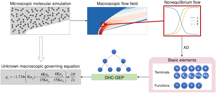
Figure 1: Flowchart of discovering unknown governing equations from data. First, macroscopic flow field data is generated via microscopic molecular simulation. Then, the basic elements preselected for DHC-GEP are constituted with state variables, mathematical operators and other variables of concern. If the basic elements include gradient terms, auto differentiation (AD) would be employed. Finally, based on the terminal and function sets, DHC-GEP continues to perform a global exploration in the space of mathematical expressions until a satisfying equation is obtained.

2 Direct simulation Monte Carlo (DSMC)

DSMC is a stochastic particle-based method, which solves the Boltzmann equation via approximating the molecular velocity distribution function with simulation molecules (Oran et al., 1998). DSMC tracks the simulation molecules, as they move, collide with other molecules and reflect from boundaries. The macroscopic gas properties, such as macroscopic velocity and density, are obtained via sampling corresponding molecular information and making an average at the computational cells.

For a specific application, DSMC first initializes the simulation molecules according to the initial distributions of density and macroscopic velocity. Then the molecular motions and inter-molecular collisions are sequentially conducted in each calculated time interval. Specifically, the molecular motions are implemented in a deterministic way. Each molecule moves ballistically from its original position to a new position, and the displacement is equal to the product of its velocity times the time step. If the trajectory crosses any boundaries, an appropriate gas-wall interaction model would be employed to determine the reflected velocity. Common gas-wall interaction models include specular, diffuse and Maxwell reflection models. In our simulations, diffuse model is employed. On the contrary, the inter-molecular collisions are implemented in a probabilistic way. Among the several algorithms for the modelling of inter-molecular collisions, the no-time-counter (NTC) technique (Bird, 1994) is most widely used. In NTC, any two molecules are selected as a collision pair in a probability that is proportional to the relative speed between them. Then, the post-collision velocities of molecules are determined by the molecular model employed. In this work we employ hard sphere (HS) model for the first two cases, Maxwell molecule model for the shock wave case and variable hard sphere (VHS) model for the Poiseuille flow case. It is noteworthy that because the above molecular motions and inter-molecular collisions are conducted in a decoupled manner, the time step needs to be smaller than the molecular mean collision time, and the cell size for the selection of collision pairs needs to be smaller than the molecular mean free path.

Theoretically, DSMC has been proved to be capable of solving the Boltzmann equation from the perspective of molecular movements (Wagner, 1992), and thus can be applied to simulate the whole regime of gas flows (Sun and Boyd, 2002; Stefanov et al., 2002; Zhang et al., 2010; Gallis et al., 2017). What is most important for this work is that DSMC does not assume any macroscopic governing equations. This makes the derived equations of DHC-GEP more convincing. The simulation details are provided in Supplementary § 2. The dataset sizes are summarized in Supplementary table 2.

3 Dimensional homogeneity constrained gene expression programming (DHC-GEP)

The flowchart of DHC-GEP is shown in figure 2(a). It starts with creating $N_{i}$ random individuals of initial population. Each individual has two forms, genotype (chromosome (CS)) and phenotype (expression tree (ET)). Phenotype is the expression product of genotype. Then, via dimensional verification, all the individuals are classified into valid ones and invalid ones according to whether they satisfy the dimensional homogeneity. The valid ones would be translated into mathematical expressions (ME), and be evaluated for losses with input data. The invalid ones would be directly assigned a significant loss, and be eliminated in the subsequent iterations. The best individual (with lowest loss) is replicated to the next generation straightly. Other individuals are selected as superior individuals in the probabilities that are inversely proportional to their losses. Based on the superior individuals, the population of next generation is reproduced via genetic operators. The common genetic operators include replication, mutation, transposition and recombination, the details of which are provided in Supplementary § 1.3. The above processes are iteratively conducted until a satisfying individual is obtained.

Each chromosome is composed of one or more genes. A specific schematic diagram of gene is shown in figure 2(b). There are two parts in a gene, i.e., head and tail. The head consists of the symbols from the function set or terminal set, while the tail only consists of symbols from terminal set. The function set and terminal set are both predefined according to the specific problem. For the problems in this work, the function set includes basic mathematical operators ($+,\;-,\;\times,\;\div$). If necessary for other problems, the function set can also include nonlinear functions like sin, cos, and even user-defined functions. The terminal set includes the symbols of variables and constants. Taking the first symbol of gene as the root node, we can translate the gene into the expression tree (shown in figure 2(b)) through level-order traversal according to the argument requirement of each function. Note that the final four symbols are not expressed, and the region before them is called open reading frame (ORF). The length of ORF is unfixed to ensure the diversity of expressed products. The derived equations can be concise or complex. On the contrary, the length of gene is fixed, preventing the individuals from bloating. Assuming the length of head is $n$, then the length of tail must be $n\times\left({h-1}\right)+1$, where $h$ is the maximum number of arguments in the functions.

The dimensional verification is the additional process to implement the constraint of dimensional homogeneity, and is introduced as follows (a simplified version is shown in figure 2(c)). The general form of governing equation is assumed as:

$$Y=f(X,\vartheta).$$ (1)

Here $Y$ is the target variable, and $f(\cdot)$ is the mathematical expression coded by chromosome. $X$ and $\vartheta$ represent variables and constants, respectively. Dimensional homogeneity means that $f(\cdot)$ should have the same dimension with $Y$, and every part in $f(\cdot)$ should satisfy the constraint that the parameters for operators $+$ or $-$ must have the same dimensions.

Generally, dimensional verification includes calculating the dimension of $f(\cdot)$ and comparing it with the dimension of $Y$. For calculating dimensions, there are five principles that should be noted.

• Computers cannot directly deal with symbolic operations, but only numerical operations.

• In International System of Units (SI), there are seven base dimensions: length ($L$), mass ($M$), time ($T$), electric current ($I$), thermodynamic temperature ($\Theta$), amount of substance ($N$) and luminous intensity ($J$). The dimensions of any other physical quantities can be derived by powers, products, or quotients of these base dimensions.

• Base dimensions are independent of each other. Anyone cannot be derived by other base dimensions.

• Physical quantities with different dimensions cannot be added or subtracted. Adding or subtracting the physical quantities with the same dimension do not change the dimension.

• When physical quantities are multiplied or divided, the corresponding dimensions are multiplied or divided equally.

Considering the above principles, we propose to assign number tags to physical quantities, and replace the dimensional calculations by numerical calculations. For the seven base dimensions, the tags are 2, 3, 5, 7, 11, 13 and 17, respectively. These numbers are prime numbers, ensuring the base dimensions being independent of each other. The tags for other physical quantities are derived according to their dimensions. For example, as the dimension of velocity is length divided by time ($L/T$), its tag is defined as $2/5$. It is noteworthy that the tags are always in the form of fractions rather than floats, to avoid truncation errors. The tags for constants and dimensionless quantities are set to $1$. Besides, according to the last two principles, we modify the operation rules of mathematical operators. The pseudo-codes are provided in Supplementary § 1.1. With the number tags and modified mathematical operators, we can compute the dimension of each node in the expression tree from the bottom up. If the parameters for one function node ($+$ or $-$) does not have the same dimension, the certain individual is directly identified as invalid one. Otherwise, we can calculate the specific dimension of the individual, i.e., the number tag for the root node. Comparing it with the tag for the target variable, we can conclude whether the certain individual is dimensional homogeneous.

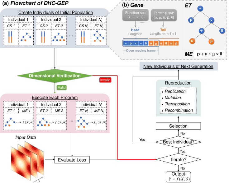
(a)

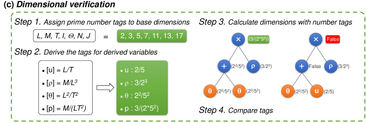
(b)

Figure 2: Main characteristics of DHC-GEP. (a) Flowchart of DHC-GEP. (b) Schematic diagram of a gene and its corresponding expression tree and mathematical expression. (c) Strategy of dimensional verification.

4 Demonstration on benchmark studies

4.1 Diffusion equation

We employ the direct simulation Monte Carlo (DSMC) method to simulate a two-dimensional diffusion flow. The details of simulation are provided in Supplementary § 2. The theoretical diffusion equation is,

$$\frac{{\partial\rho}}{{\partial t}}=D\frac{{{\partial^{2}}\rho}}{{\partial{y^{2}}}}.$$ (2)

Here $D$ is the diffusion coefficient and equals to $2.47\times{10^{-5}}\;{{\rm m}^{2}}{{\rm s}^{-1}}$ for the argon gas in our simulation.

Before using the dataset generated by DSMC, we test DHC-GEP and Original-GEP on clean dataset. The only difference between the DSMC dataset and the clean dataset lies in the target variable ($\frac{{\partial\rho}}{{\partial t}}$). In the clean dataset, $\frac{{\partial\rho}}{{\partial t}}$ is directly determined based on $D$ and $\frac{{{\partial^{2}}\rho}}{{\partial{y^{2}}}}$, according to (2). We define the function set as $\left\{{+,-,\times,\div}\right\}$, and the terminal set as $\left\{{D,\frac{{\partial\rho}}{{\partial y}},\frac{{{\partial^{2}}\rho}}{{\partial{y^{2}}}}{\rm{,}}\frac{{{\partial^{3}}\rho}}{{\partial{y^{3}}}}}\right\}$. All the important hyperparameters are set to the same for both GEP methods (see in table 1). The derived equations are shown in table 2. It can be seen that the derived equation of DHC-GEP is consistent with the theoretical equation, while the derived equation of Original-GEP is partially correct. Specifically, Original-GEP identify the right function form and coefficient ($2.47\times{10^{-5}}$) that is numerically equal to the diffusion coefficient. In the view of data fitting, this is a correct result. However, this equation is not dimensional homogeneous, and does not reflect the real physical mechanism (i.e., cannot identify the coefficient ($2.47\times{10^{-5}}$) as the diffusion coefficient). For another diffusion flow with a different diffusion coefficient, the derived equation of Original-GEP is no longer valid, while the derived equation of DHC-GEP is generally applicable.

Table 1: Important hyperparameters of DHC-GEP.

Case	Length of head	Number of genes in a chromosome	Number of individuals in a population
Diffusion problem	3	1	120
Taylor-Green vortex	5	2	500
Flow around a cylinder	5	2	500
One-dimensional shock wave	15	2	1660
Rarefied Poiseuille flow	15	2	1660

Table 2: Derived equations of DHC-GEP.

Case	Theoretical equation	Data	Method	Derived equation	Loss
[1pt/1pt]Diffusion problem	$\begin{array}[]{l}\frac{{\partial\rho}}{{\partial t}}=D\frac{{{\partial^{2}}\rho}}{{\partial{y^{2}}}},\\ D=2.47\times{10^{-5}}\;{{\rm m}^{2}}{{\rm s}^{-1}}\end{array}$	Clean dataset	DHC-GEP	$\frac{{\partial\rho}}{{\partial t}}=1.0D\frac{{{\partial^{2}}\rho}}{{\partial{y^{2}}}}$	0
4-6[1pt/1pt]			Original-GEP	$\frac{{\partial\rho}}{{\partial t}}=2.47\times{10^{-5}}\frac{{{\partial^{2}}\rho}}{{\partial{y^{2}}}}$	0
3-6[1pt/1pt]		DSMC dataset	DHC-GEP	$\frac{{\partial\rho}}{{\partial t}}=0.999D\frac{{{\partial^{2}}\rho}}{{\partial{y^{2}}}}$	0.165
4-6[1pt/1pt]			Original-GEP	$\frac{{\partial\rho}}{{\partial t}}=0.997\left({D\frac{{{\partial^{2}}\rho}}{{\partial{y^{2}}}}+\frac{{\partial\rho}}{{\partial y}}-\rho}\right)$	0.135
[1pt/1pt] Taylor-Green vortex	$\begin{array}[]{l}\frac{{\partial{\omega_{z}}}}{{\partial t}}=\upsilon\left({\frac{{{\partial^{2}}{\omega_{z}}}}{{\partial{x^{2}}}}+\frac{{{\partial^{2}}{\omega_{z}}}}{{\partial{y^{2}}}}}\right)-\left({u\frac{{\partial{\omega_{z}}}}{{\partial x}}+v\frac{{\partial{\omega_{z}}}}{{\partial y}}}\right),\\ \upsilon=15.44\;{{\rm m}^{2}}{{\rm s}^{-1}}\end{array}$	Clean dataset	DHC-GEP	$\frac{{\partial{\omega_{z}}}}{{\partial t}}=1.0\upsilon\left({\frac{{{\partial^{2}}{\omega_{z}}}}{{\partial{x^{2}}}}+\frac{{{\partial^{2}}{\omega_{z}}}}{{\partial{y^{2}}}}}\right)$	0
4-6[1pt/1pt]			Original-GEP	$\frac{{\partial{\omega_{z}}}}{{\partial t}}=15.44\left({\frac{{{\partial^{2}}{\omega_{z}}}}{{\partial{x^{2}}}}+\frac{{{\partial^{2}}{\omega_{z}}}}{{\partial{y^{2}}}}}\right)$	0
3-6[1pt/1pt]		DSMC dataset	DHC-GEP	$\frac{{\partial{\omega_{z}}}}{{\partial t}}=0.981\upsilon\left({\frac{{{\partial^{2}}{\omega_{z}}}}{{\partial{x^{2}}}}+\frac{{{\partial^{2}}{\omega_{z}}}}{{\partial{y^{2}}}}}\right)$	0.112
4-6[1pt/1pt]			Original-GEP	$\frac{{\partial{\omega_{z}}}}{{\partial t}}=-3.916{\left({\upsilon\frac{{\partial v}}{{\partial x}}\left({v+\frac{{{\partial^{2}}{\omega_{z}}}}{{\partial{x^{2}}}}}\right)-\frac{1}{5}\frac{{{\partial^{2}}{\omega_{z}}}}{{\partial{x^{2}}}}}\right)}\bigg{/}{\left({v+\frac{{{\partial^{2}}{\omega_{z}}}}{{\partial{x^{2}}}}}\right)}$	0.096
[1pt/1pt] Flow around a cylinder	$\begin{array}[]{l}\frac{{\partial{\omega_{z}}}}{{\partial t}}=\upsilon\left({\frac{{{\partial^{2}}{\omega_{z}}}}{{\partial{x^{2}}}}+\frac{{{\partial^{2}}{\omega_{z}}}}{{\partial{y^{2}}}}}\right)-\left({u\frac{{\partial{\omega_{z}}}}{{\partial x}}+v\frac{{\partial{\omega_{z}}}}{{\partial y}}}\right),\\ \upsilon=0.01\;{{\rm m}^{2}}{{\rm s}^{-1}}\end{array}$	CFD dataset	DHC-GEP	$\frac{{\partial{\omega_{z}}}}{{\partial t}}=0.989\upsilon\left({\frac{{{\partial^{2}}{\omega_{z}}}}{{\partial{x^{2}}}}+\frac{{{\partial^{2}}{\omega_{z}}}}{{\partial{y^{2}}}}}\right)-0.989\left({u\frac{{\partial{\omega_{z}}}}{{\partial x}}+v\frac{{\partial{\omega_{z}}}}{{\partial y}}}\right)$	0.049
4-6[1pt/1pt]			Original-GEP	$\frac{{\partial{\omega_{z}}}}{{\partial t}}=0.014\frac{{\partial{\omega_{z}}}}{{\partial x}}\left({7\frac{{\partial{\omega_{z}}}}{{\partial y}}-\frac{{{\partial^{2}}v}}{{\partial{x^{2}}}}\frac{{\partial{\omega_{z}}}}{{\partial y}}-\frac{{{\partial^{2}}{\omega_{z}}}}{{\partial{y^{2}}}}-70u}\right)$	0.032

Subsequently, we test DHC-GEP and Original-GEP on the DSMC dataset. All settings are consistent with those in the test on clean dataset. The derived equations are shown in table 2. The coefficient of the equation discovered by DHC-GEP has a minor deviation with that of the theoretical equation, and the loss is not perfectly zero. This is because DSMC is a stochastic particle-based method, the data of which is inherently noisy. It is impossible for DSMC to simulate a flow with the diffusion coefficient being exact $2.47\times{10^{-5}}\;{{\rm m}^{2}}{{\rm s}^{-1}}$. Small fluctuations around the theoretical value are acceptable. Besides, calculating derivatives also introduces errors. Therefore, we believe that DHC-GEP has discovered the correct equation. On the contrary, the derived equation of Original-GEP is wrong. As the loss is even smaller than that of the correct equation derived by DHC-GEP, this equation is obviously overfitting to noise.

More importantly, the result of DHC-GEP is insensitive to hyperparameters. Despite we adjust the length of head in genes and the number of individuals in a population, DHC-GEP is always capable of discovering the correct equations. The underlying reason is that the dimensional homogeneity plays a great constraint role. The overfitting results would be automatically filtered out due to not satisfying the dimensional homogeneity. On the contrary, Original-GEP always favors the equations with smaller loss, so it tends to converge to overfitting results if data is noisy. Our numerical experiences show that Original-GEP may discover the correct equations only when tuning the hyperparameters repeatedly and terminating the evolution at a mediate generation (when overfitting equations have not appeared).

We compare the computational cost required per 1 000 generations of evolution. Based on the 3.5GHz Intel Xeon E5-1620 processor, the average CPU runtime of Original-GEP (443 seconds) is almost twice that of DHC-GEP (216 seconds). The main reason is that DHC-GEP can identify some individuals as invalid ones through dimensional verification and then skip the process of evaluating losses for these individuals. It can still save computational time despite of the extra expense on the dimensional verification. Furthermore, as the complexity of problem increases, the number of invalid individuals increases, so the advantage of computational efficiency of DHC-GEP becomes more significant.

4.2 Vorticity transport equation

We employ DSMC to simulate the temporal evolution of Taylor-Green vortex, shown in figure 3(a). The theoretical governing equation is vorticity transport equation,

$$\frac{{\partial{\omega_{z}}}}{{\partial t}}=\upsilon\left({\frac{{{\partial^{2}}{\omega_{z}}}}{{\partial{x^{2}}}}+\frac{{{\partial^{2}}{\omega_{z}}}}{{\partial{y^{2}}}}}\right)-\left({u\frac{{\partial{\omega_{z}}}}{{\partial x}}+v\frac{{\partial{\omega_{z}}}}{{\partial y}}}\right).$$ (3)

Here, $u$ and $v$ are the velocities in the $x$ and $y$ directions, respectively. ${\omega_{z}}$ is the vorticity in the $z$ direction. $\upsilon$ is the kinematic viscosity, and approximately equals to $15.44\;{{\rm m}^{2}}{{\rm s}^{-1}}$ for argon gas at standard condition. Compared with the diffusion equation (2), this equation is more complex, involving multiple variables and nonlinear terms.

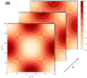
(a)

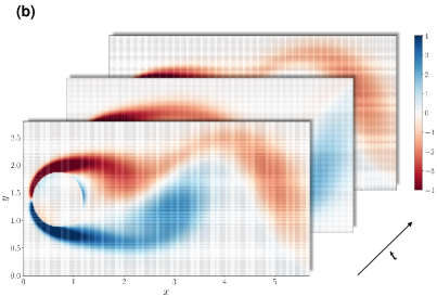
(b)

Figure 3: Temporal evolution of vorticity. (a) Taylor-Green vortex at the instants of $t=0,100\tau,\;200\tau.$ Here, $\tau$ and $\lambda$ are the mean collision time and mean free path of argon gas molecules at standard condition, respectively. (b) Viscous flow around a cylinder at the instants of $t=0\;{\rm s},3\;{\rm s},\;6\;{\rm s}.$

In this case, we define the target variable as $\frac{{\partial{\omega_{z}}}}{{\partial t}}$, the function set as $\left\{{+,-,\times,\div}\right\}$, and the terminal set as $\left\{{\mu,u,v,\omega_{z},\frac{{\partial u}}{{\partial x}},\frac{{{\partial^{2}}u}}{{\partial{x^{2}}}},\frac{{\partial u}}{{\partial y}},\frac{{{\partial^{2}}u}}{{\partial{y^{2}}}},\frac{{\partial v}}{{\partial x}},\frac{{{\partial^{2}}v}}{{\partial{x^{2}}}},\frac{{\partial v}}{{\partial y}},\frac{{{\partial^{2}}v}}{{\partial{y^{2}}}},\frac{{\partial\omega_{z}}}{{\partial x}},\frac{{{\partial^{2}}\omega_{z}}}{{\partial{x^{2}}}},\frac{{\partial\omega_{z}}}{{\partial y}},\frac{{{\partial^{2}}\omega_{z}}}{{\partial{y^{2}}}}}\right\}$. A large number of distraction terms are introduced to enhance the test difficulty.The hyperparameters of both GEP methods are summarized in table 1.

We also test the performances of DHC-GEP on the clean dataset and the DSMC dataset sequentially. The results are provided in table 2. An interesting observation is that the derived equations of DHC-GEP miss two convective terms $\left({u\frac{{\partial{\omega_{z}}}}{{\partial x}},v\frac{{\partial{\omega_{z}}}}{{\partial y}}}\right)$. This is caused by the unique feature of Taylor-Green vortex. The analytical expression of Taylor-Green vortex is

$$\begin{array}[]{*{35}{l}}u=v_{0}\cdot{\rm cos}\left(x\right){\rm sin}\left(y\right){\exp\left({-2\upsilon t}\right)\vspace{0.8ex}}\\ v=-v_{0}\cdot{\rm sin}\left(x\right){\rm cos}\left(y\right){\exp\left({-2\upsilon t}\right)\vspace{0.8ex}}\\ {{\omega_{z}}}=-2v_{0}\cdot{\rm cos}\left(x\right){\rm cos}\left(y\right){\exp\left({-2\upsilon t}\right)}\end{array},$$ (4)

where ${v_{0}}$ is the initial amplitude of velocity. Substituting (4) into the convective terms $\left({u\frac{{\partial{\omega_{z}}}}{{\partial x}},v\frac{{\partial{\omega_{z}}}}{{\partial y}}}\right)$, it is clear that the sum of convective terms is automatically zero. Therefore, the equations without convective terms are also correct for the Taylor-Green vortex. The superiorities of DHC-GEP in discovering the vorticity transport equation are similar to those in the previous case, so not repeated here.

To discover the complete vorticity transport equation and validate the performance of DHC-GEP on discovering nonlinear terms, we further consider a viscous flow around a cylinder at Reynolds number being 100, shown in figure 3(b). The dataset is the open access dataset provided by Rudy et al. (2017), and the theoretical governing equation is

$$\frac{{\partial{\omega_{z}}}}{{\partial t}}=0.01\cdot\left({\frac{{{\partial^{2}}{\omega_{z}}}}{{\partial{x^{2}}}}+\frac{{{\partial^{2}}{\omega_{z}}}}{{\partial{y^{2}}}}}\right)-\left({u\frac{{\partial{\omega_{z}}}}{{\partial x}}+v\frac{{\partial{\omega_{z}}}}{{\partial y}}}\right).$$ (5)

For the sake of simplicity, we regard the data as dimensional data with its kinematic viscosity $\upsilon=0.01\;{{\rm m}^{2}}{{\rm s}^{-1}}$. The hyperparameters of both GEP methods are consistent with those in the case of Taylor-Green vortex. The results are provided in table 2. DHC-GEP discovers the correct and complete vorticity transport equation. Note that we only subsample 100 data points to conduct the test, while 300 000 data points are employed in Rudy et al. (2017). This demonstrates the improved performance of DHC-GEP on discovering equations from scarce data. Generally, if the size of dataset is small, the information carried by data is sparse, leading to the derived equations overfitting to partial phenomena. As a result, for other methods, a dataset with big size is generally required to avoid overfitting. However, in DHC-GEP, the overfitting equations are automatically filtered out by the constraint of dimensional homogeneity.

5 Application on discovering unknown constitutive relations

The general governing equations for fluid flows are the conservation equations of mass, momentum and energy as follows,

$$\begin{array}[]{*{35}{l}}\frac{{D\rho}}{{Dt}}+\rho\frac{{\partial{v_{k}}}}{{\partial{x_{k}}}}=0,\vspace{0.8ex}\\ \rho\frac{{D{v_{i}}}}{{Dt}}+\frac{{\partial p}}{{\partial{x_{i}}}}+\frac{{\partial{\tau_{ik}}}}{{\partial{x_{k}}}}=\rho{F_{i}},\vspace{0.8ex}\\ \frac{3}{2}\frac{{D\theta}}{{Dt}}+\frac{{\partial{q_{k}}}}{{\partial{x_{k}}}}=-\left({p{\delta_{ij}}+{\tau_{ij}}}\right)\frac{{\partial{v_{i}}}}{{\partial{x_{j}}}}.\end{array}.$$ (6)

Here, $\frac{D}{{Dt}}{\rm{=}}\frac{\partial}{{\partial t}}{\rm{+}}{v_{i}}\frac{\partial}{{\partial{x_{i}}}}$ is the substantial derivative, and $\theta=\frac{k}{m}T$ is the temperature in $energy/mass$ unit. Besides the five conservative variables $\rho$, ${v_{i}}$ and $\theta$, there are eight additional variables, i.e., the viscous stress ${\tau_{ij}}$ and heat flux ${q_{i}}$. To numerically solve (6), the additional constitutive relations that close the viscous stress and heat flux are required. In the continuum regime, the NSF equations are widely employed, which assumes that the viscous stress/heat flux is linearly proportional to the local strain rate/temperature gradient. However, for strong non-equilibrium flows, the NSF equations are not valid (Boyd et al., 1995).

Alternatively, high-order constitutive relations have been derived from the Boltzmann equation using the Chapman-Enskog method (Chapman and Cowling, 1990), including Burnett equations (Burnett, 1936), super-Burnett equations (Shavaliyev, 1993) and augmented-Burnett equations (Zhong et al., 1993), to account for the non-equilibrium effects. However, despite being proved to be superior to NSF equations, these equations are still unsatisfactory in strong non-equilibrium flows. In this work, we employ DHC-GEP to discover the unknown constitutive relations in two typical non-equilibrium flows, as the examples to illustrate how to apply DHC-GEP to discover unknown governing equations.

5.1 One-dimensional shock wave

In the research community of non-equilibrium flows, one-dimensional shock wave is a benchmark to validate solvers and formulations in numerical computations. We employ DSMC to simulate the one-dimensional shock wave of argon gas, the general structure of which is shown in figure 4. The details of simulation are introduced in Supplementary § 2.

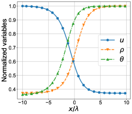
Figure 4: General structure of one-dimensional shock. Each variable is normalized with its maximum value in the computational domain.

In this case, the target variable is defined as the heat flux in the $x$ direction (${q_{x}}$). The function set is defined as $\left\{{+,-,\times,\div}\right\}$ as usual, while the terminal set is elaborately constructed to embed physics knowledge as follows.

• Constitutive relations describe the local transport mechanisms of momentum and energy, and hence we regard local non-equilibrium parameters as key factors. Specifically, the gradient-length local (GLL) Knudsen number defined as $K{n_{Q}}=\frac{{{\lambda_{l}}}}{Q}\nabla Q$ is selected. The local non-equilibrium characteristics intensify as the increase of the absolute value of $K{n_{Q}}$. Here, ${\lambda_{l}}$ is the local mean free path, and $Q$ represents state variables, including temperature ($\theta$) and density ($\rho$).

• The transports of momentum and energy are driven by the gradients of state variables. As a result, the gradient terms are selected, including $\frac{{\partial u}}{{\partial x}},\frac{{\partial\rho}}{{\partial x}},\frac{{\partial\theta}}{{\partial x}},\frac{{{\partial^{2}}u}}{{\partial{x^{2}}}},\frac{{{\partial^{2}}\rho}}{{\partial{x^{2}}}},\frac{{{\partial^{2}}\theta}}{{\partial{x^{2}}}},\frac{{{\partial^{3}}u}}{{\partial{x^{3}}}},\frac{{{\partial^{3}}\rho}}{{\partial{x^{3}}}}$ and $\frac{{{\partial^{3}}\theta}}{{\partial{x^{3}}}}$.

• The state variables themselves are important factors. Besides, it is noteworthy that the constitutive relations should satisfy Galilean invariance (Han et al., 2019; Li et al., 2021), which means that the constitutive relations cannot contain velocity ($u$) explicitly outside the partial differential operators. The proof is provided in Appendix C. Therefore, the state variables ($\theta$ and $\rho$) excluding velocity are selected. This is also the reason for that we do not select the GLL Knudsen number of velocity.

• The parameters representing the physical properties of gas are selected, including local viscosity ($\mu$) , local heat conductivity ($\kappa$) , heat capacity ratio ($\gamma=5/3$ for argon gas) and viscosity exponent ($\omega=1$ for Maxwell molecules).

Finally, the terminal set is $\left\{{K{n_{\theta}},K{n_{\rho}},\frac{{\partial u}}{{\partial x}},\frac{{\partial\rho}}{{\partial x}},\frac{{\partial\theta}}{{\partial x}},\frac{{{\partial^{2}}u}}{{\partial{x^{2}}}},\frac{{{\partial^{2}}\rho}}{{\partial{x^{2}}}},\frac{{{\partial^{2}}\theta}}{{\partial{x^{2}}}},\frac{{{\partial^{3}}u}}{{\partial{x^{3}}}},\frac{{{\partial^{3}}\rho}}{{\partial{x^{3}}}},\frac{{{\partial^{3}}\theta}}{{\partial{x^{3}}}},\rho,\theta,\mu,\kappa,\gamma,\omega}\right\}$.

We employ DHC-GEP to discover the underlying constitutive relation based on the data of two cases with the freestream Mach number $M{a_{\infty}}=3.0$ and $4.0$. After 4,158 generations, a satisfying equation is discovered,

$${q_{x}}=-1.734\left({K{n_{\rho}}\gamma+\frac{{4K{n_{\theta}}}}{{15K{n_{\rho}}}}+\frac{{4K{n_{\rho}}}}{{15K{n_{\theta}}}}}\right)\kappa\frac{{\partial\theta}}{{\partial x}}.$$ (7)

We compare the results predicted by (7) with those predicted by NSF equation, Burnett equation, augmented-Burnett equation and super-Burnett equation in figure 5. Besides, we define the relative error as

$$error=\frac{{\sqrt{\sum\limits_{i=1}^{N}{{{\left({{{\hat{q}}_{x,i}}-{q_{x,i}}}\right)}^{2}}}}}}{{\sqrt{\sum\limits_{i=1}^{N}{q_{x,i}^{2}}}}},$$ (8)

where the variable with a superscript $\wedge$ is the prediction variable, and $N$ is the number of data points. The relative errors for each constitutive relation are summarized in table 3. It can be found that the derived constitutive relation of DHC-GEP is much more accurate than other equations in a wide range of $M{a_{\infty}}$, and is applicable to the scenarios of interpolation and extrapolation to some extent.

Table 3: Relative errors of the derived equation of DHC-GEP, NSF equation, Burnett equation, augmented-Burnett equation (Au-Burnett) and super-Burnett equation (Su-Burnett) for the one-dimensional shock wave case.

	$M{a_{\infty}}=2.0$	$M{a_{\infty}}=2.3$	$M{a_{\infty}}=2.5$	$M{a_{\infty}}=3.0$	$M{a_{\infty}}=3.2$	$M{a_{\infty}}=3.5$	$M{a_{\infty}}=4.0$	$M{a_{\infty}}=4.2$	$M{a_{\infty}}=4.5$	$M{a_{\infty}}=5.0$	$M{a_{\infty}}=5.5$
DHC-GEP	0.099	0.092	0.086	0.057	0.053	0.046	0.041	0.043	0.045	0.050	0.054
NSF	0.251	0.321	0.357	0.431	0.451	0.477	0.509	0.518	0.530	0.545	0.555
Burnett	0.120	0.150	0.164	0.204	0.219	0.238	0.266	0.274	0.284	0.298	0.306
Au-Burnett	0.127	0.164	0.180	0.221	0.237	0.257	0.284	0.293	0.303	0.316	0.325
Su-Burnett	0.206	0.255	0.282	0.333	0.349	0.370	0.396	0.406	0.415	0.428	0.437

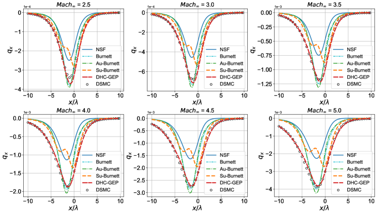
Figure 5: Comparisons of NSF equation, Burnett equation, augmented-Burnett equation (Au-Burnett), super-Burnett equation (Su-Burnett), the derived equation of DHC-GEP and DSMC (exact solution) at $M{a_{\infty}}=2.5,\;3.0,\;3.5,\;4.0,\;4.5$ and $5.0$ for the one-dimensional shock wave case.

Furthermore, as the derived model is explicitly expressed, its physical properties can be checked. Obviously, it satisfies the Galilean invariance, as no velocity ($u$) explicitly appears outside the partial differential operators. Besides, we can also prove that it satisfies the second law of thermodynamics, which is critical for physical laws. Theoretically, whether a constitutive relation satisfies the second law of thermodynamics can be determined through the Clausius-Duhem inequality (Comeaux, 1995)

$$\rho\frac{{D{s_{eq}}}}{{Dt}}+\nabla\cdot\frac{\mathbf{q}}{\theta}=-\frac{1}{\theta}\mathbf{\tau}:\nabla\mathbf{v}-\frac{1}{{{\theta^{2}}}}\mathbf{q}\cdot\nabla\theta\geq 0.,$$ (9)

The two terms on the left side are local increase rate of entropy and reversible outflow of entropy, respectively. The second law of thermodynamics requires that the sum of the two terms on the right side, which are called entropy production, must be non-negative. For our case, this is simplified as

$$1.734\frac{1}{{{\theta^{2}}}}\left({K{n_{\rho}}\gamma+\frac{{4K{n_{\theta}}}}{{15K{n_{\rho}}}}+\frac{{4K{n_{\rho}}}}{{15K{n_{\theta}}}}}\right)\kappa{\left({\frac{{\partial\theta}}{{\partial x}}}\right)^{2}}\geq 0.$$ (10)

According to figure 4, for one-dimensional shock wave, the gradients of density and temperature are non-negative. Therefore, both $K{n_{\rho}}$ and $K{n_{\theta}}$ are non-negative, and (10) naturally holds. As a comparison, whether Burnett equation, super-Burnett equation and augmented-Burnett equation satisfy the second law of thermodynamics is obscure (Comeaux, 1995).

5.2 Rarefied Poiseuille flow

Poiseuille flow is a flow confined between two infinite, parallel and static plates. The gas is driven by a constant external force in the $x$ direction. A schematic diagram of Poiseuille flow is shown in figure 6. The global Knudsen number is defined as $Kn=\frac{\lambda}{H}$, where $H$ is the distance between two plates, and $\lambda$ is the mean free path of the argon gas molecules at standard condition. We employ DSMC to simulate the Poiseuille flows at $Kn=0.01,\;0.1,\;0.2,\;0.3,\;0.35,\;0.4,\;0.5$ and $0.6$.

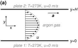
(a)

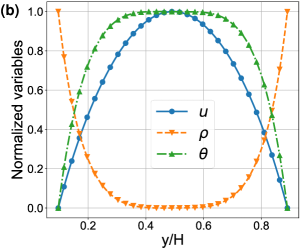
(b)

Figure 6: (a) Schematic diagram of Poiseuille flow. (b) Profiles of velocity, density and temperature along the direction normal to the plate. Each variable ($U$) is normalized with ${U_{{\rm Normal}}}=\left({U-{U_{\min}}}\right)/\left({{U_{\max}}-{U_{\min}}}\right)$.

In this case, the target variable is defined as the viscous shear stress (${\tau_{xy}}$), and the function set is defined as $\left\{{+,-,\times,\div}\right\}$. The terminal set is almost the same with that in the case of one-dimensional shock wave, i.e., $\left\{{K{n_{\theta}},K{n_{\rho}},\frac{{\partial u}}{{\partial y}},\frac{{\partial\rho}}{{\partial y}},\frac{{\partial\theta}}{{\partial y}},\rho,\theta,\mu,\gamma,\omega}\right\}$ , except that the high-order gradients are removed. The motivation for removing high-order gradients is that the derived constitutive relation should be applicable in CFD. If containing high-order gradients, the constitutive relation would be unstable and require additional boundary conditions (Zhong et al., 1993; Bobylev, 1982; Struchtrup and Torrilhon, 2003; Torrilhon and Struchtrup, 2004; Singh et al., 2017), which are the common problems with the kind of Burnett equations.

We employ DHC-GEP to discover the underlying constitutive relation based on the data at $Kn=0.01,\;0.3$ and $0.4$. After 30 742 generations, a satisfying equation is discovered,

$${\tau_{xy}}=-0.247\left({\frac{5}{{Kn_{\rho}^{2}+\gamma}}-\frac{{K{n_{\theta}}}}{{K{n_{\rho}}}}}\right)\mu\frac{{\partial u}}{{\partial y}}.$$ (11)

We compare the results predicted by (11) with those predicted by NSF equation, Burnett equation, augmented-Burnett equation and super-Burnett equation in figure 7. The relative errors for each constitutive relation are summarized in table 4. It can be found that the derived constitutive relation of DHC-GEP is much more accurate than other equations in a wide range of $Kn$, and is applicable to the scenarios of interpolation ($Kn\leq\;0.4$) and extrapolation ($0.4<Kn\leq\;0.6$).

Table 4: Relative errors of the derived equation of DHC-GEP, NSF equation, Burnett equation, augmented-Burnett equation (Au-Burnett) and super-Burnett equation (Su-Burnett) for the rarefied Poiseuille flow case. Note that the NSF equation is equal to the Burnett equation in this case.

	$Kn=0.01$	$Kn=0.1$	$Kn=0.2$	$Kn=0.3$	$Kn=0.35$	$Kn=0.4$	$Kn=0.5$	$Kn=0.6$
DHC-GEP	0.028	0.083	0.044	0.019	0.025	0.039	0.076	0.137
NSF/Burnett	0.029	0.659	0.844	1.233	1.426	1.606	1.963	2.318
Au-Burnett	0.029	0.594	0.697	0.805	0.783	0.687	0.264	0.667
Su-Burnett	0.030	0.921	1.435	2.948	4.012	5.306	9.045	14.000

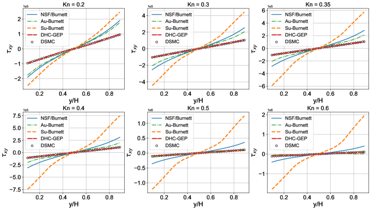
Figure 7: Comparisons of NSF equation, Burnett equation, augmented-Burnett equation (Au-Burnett), super-Burnett equation (Su-Burnett), the derived equation of DHC-GEP and DSMC (exact solution) at $Kn=0.2,\;0.3,\;0.35,\;0.4,\;0.5$ and $0.6$ for the rarefied Poiseuille flow case. Note that the NSF equation is equal to the Burnett equation in this case.

Note that for continuum flows, the GLL Knudsen numbers ($K{n_{\rho}}$ and $K{n_{\theta}}$) approach zero, and (11) reduces to

$${\tau_{xy}}=-0.247\left({\frac{5}{\gamma}-\frac{{K{n_{\theta}}}}{{K{n_{\rho}}}}}\right)\mu\frac{{\partial u}}{{\partial y}}=-0.247\left({3-\frac{{K{n_{\theta}}}}{{K{n_{\rho}}}}}\right)\mu\frac{{\partial u}}{{\partial y}}.$$ (12)

Here we have used the value of $\gamma=5/3$ for monatomic gas in the above equation. For the Poiseuille flow in the continuum regime, the pressure along the $y$ direction tends to be constant. Taking the flow of $Kn=0.01$ as an example, the pressure oscillates about $0.5\;\%$ of its absolute value. Considering the ideal gas equation of state $\rho=\frac{p}{\theta}$, we can get

$$\partial\rho=-\frac{p}{{{\theta^{2}}}}\partial\theta=-\frac{\rho}{\theta}\partial\theta.$$ (13)

Then, combining (13) with $K{n_{\rho}}=\frac{{{\lambda_{l}}}}{\rho}\frac{{\partial\rho}}{{\partial y}}$ and $K{n_{\theta}}=\frac{{{\lambda_{l}}}}{\theta}\frac{{\partial\theta}}{{\partial y}}$, we can conclude $\frac{{K{n_{\theta}}}}{{K{n_{\rho}}}}=\frac{{\partial\theta}}{{\partial\rho}}\cdot\frac{\rho}{\theta}=-1$.Substituting this relation into (12) yields

$${\tau_{xy}}=-0.247\left({3+1}\right)\mu\frac{{\partial u}}{{\partial y}}\approx-\mu\frac{{\partial u}}{{\partial y}}.$$ (14)

Therefore, it can be concluded that in the continuum regime, the derived constitutive relation of DHC-GEP can be reduced to NSF equations. This makes it applicable to real complex flow problems, where flows tend to be multiscale, i.e., consisting of both continuum flows and non-equilibrium flows.

We can also prove that the derived constitutive relation of DHC-GEP satisfies the Galilean invariance and the second law of thermodynamics. Specifically, no velocity ($u$) explicitly appears outside the partial differential operators. Besides, the Clausius-Duhem inequality for this case can be simplified as

$$0.247\frac{1}{\theta}\left({\frac{5}{{Kn_{\rho}^{2}+\gamma}}-\frac{{K{n_{\theta}}}}{{K{n_{\rho}}}}}\right)\mu{\left({\frac{{\partial u}}{{\partial y}}}\right)^{2}}\geq 0.$$ (15)

According to the profile of Poiseuille flow shown in figure 6(b), the gradients of density and temperature have opposite signs. Therefore, $-\frac{{K{n_{\theta}}}}{{K{n_{\rho}}}}$ is always non-negative, and (15) naturally holds.

Finally, we emphasize that as only containing the first-order gradient of velocity, the derived constitutive relation is stable and requires the same boundary conditions with NSF equations. It is convenient to embed it into the well-developed CFD frameworks with minor modification.

6 Conclusions and discussions

A novel DHC-GEP method is proposed to discover governing equations from noisy and scarce data. The constraint of dimensional homogeneity is introduced to the Original-GEP method through an additional dimensional verification process. The major characteristics of Original-GEP are not changed, including the structure of chromosomes, the rules of expression, selection and reproduction. Therefore, DHC-GEP inherits the advantages of Original-GEP. Specifically, DHC-GEP discovers the forms of functions and their corresponding coefficients simultaneously, without any prior knowledge to assume candidate functions in advance, leading to great flexibility. The chromosomes in DHC-GEP have fixed length, avoiding bloating and unaffordable computational cost that are common in other evolutionary algorithms when dealing with high-dimensional problems. On the other hand, the length of open reading frame is unfixed, ensuring the strong expressivity. DHC-GEP is tested on two benchmarks, including diffusion equation and vorticity transport equation. It is demonstrated that DHC-GEP is capable of discovering the right equations from both the views of data fitting and uncovering physical mechanisms, and the result of DHC-GEP is robust to the hyperparameters of models, the noise level and the size of datasets. When the data is noisy or scarce, Original-GEP tends to converge to overfitting results, as they have lower loss. However, these overfitting results can be automatically filtered out in DHC-GEP. Moreover, DHC-GEP is more computationally economical than Original-GEP, as DHC-GEP can identify some individuals as invalid ones through dimensional verification and skip the process of evaluating losses for these individuals. The total cost decreases despite of the extra expense on the dimensional verification. These advantages make DHC-GEP applicable to discover the unknown governing equations in the fields where large-scale and high-fidelity datasets are intractable to obtain, such as non-equilibrium flows, turbulence and non-Newton fluids.

We also present how to employ DHC-GEP to discover the unknown constitutive relations for two typical non-equilibrium flows, including one-dimensional shock wave and rarefied Poiseuille flow. We generate the datasets by DSMC, which does not assume any governing equations. For other scientific and engineering disciplines, the datasets could be generated by experiments or first principle calculations without any assumptions of governing equations. Then, we elaborately construct the terminal set to embed relevant physics knowledge. Finally, based on the terminal and function sets, DHC-GEP continues to do a global exploration in the space of mathematical expressions until a satisfying equation is obtained. For the two cases in our work, the derived constitutive relations are much more accurate than the conventional equations derived based on physics knowledge and phenomenological assumptions (including NSF, Burnett, augmented-Burnett and super-Burnett equations) in a wide range of Knudsen number and Mach number, including both interpolation and extrapolation to some extent. Besides, the physical properties of the derived constitutive relations are excellent. Specifically, the derived constitutive relations only contain the first order gradients, and hence are stable and require the same boundary conditions with NSF equations. What is even more remarkable is that the derived constitutive relations can be proved to satisfy the Galilean invariance and the second law of thermodynamics. As a comparison, the kind of Burnett equations are unstable, and cannot be exactly proved to satisfy the second law of thermodynamics.

It should be noted that there are still several limitations that deserve further investigation. Firstly, the dimensional homogeneity is an extremely strong constraint, but not an absolute constraint that is capable of filtering out all the overfitting equations. We cannot deny that there is a very small possibility to get an overfitting equation that satisfies the dimensional homogeneity as well. In this rare case, employing multiple datasets can help. Overfitting equations are generally dataset-specific. One overfitting equation may be able to describe one specific dataset well, but definitely cannot describe multiple datasets.

Secondly, it is difficult for the present strategy (singly employing DHC-GEP) to discover a real universal governing equation. For example, the derived constitutive relation in the case of rarefied Poiseuille flow is definitely not universally valid for any non-equilibrium flows. Because this equation is essentially a model equation for a specific class of flows, the flow characteristics of which are similar to the Poiseuille flow, instead of the real universal constitutive relation. Considering the non-equilibrium transport being complex, it is believed that the real universal constitutive relation tends to be correspondingly complex, for instance containing high-order gradients. Although such constitutive relation is accurate, it is difficult or even impossible to embed it into the present frameworks of CFD. Therefore, it is not suitable for practical engineering applications. Alternatively, we should focus on the model equations, each of which is valid for a specific class of problem and is easy to be used in practice.

One promising direction is combining the clustering algorithms (Schmid et al., 2011; Callaham et al., 2021) with DHC-GEP. Based on a complex flow that contains a variety of flow characteristics, the clustering algorithms can be first employed to divide the flow into several sub-flows. Then DHC-GEP is employed in each sub-flow to discover the corresponding model equations. The derived constitutive relations in the present work are two examples of all model equations. During specific numerical computation, for each mesh point, we can first determine which sub-flow it belongs to, and then apply corresponding model equations. It is noteworthy that although the above discussions are based on non-equilibrium constitutive equations, they can also be extended to other fields.

Appendix A Loss function

We define two loss functions to evaluate the loss of individuals. One is the mean relative error (MRE) as

$${L_{MRE}}=\frac{1}{N}\sum\limits_{i=1}^{N}{\left|{\frac{{{{\hat{Y}}_{i}}-{Y_{i}}}}{{{Y_{i}}}}}\right|}.$$ (16)

Here, the variable with a superscript $\wedge$ is the prediction variable, and $N$ is the number of data points. Using MRE means that each data point is considered equally important during training, so it is suitable to be applied in scenarios where the magnitude difference of data points is large.

However, if there are more data points that are very close to zero in the dataset, MRE would fail, because for such data points a minor deviation (such as computer truncation error) would introduce significant relative error. In this way, the derived equations tend to have bad performance in the data points with high magnitude. To deal with this issue, we define the second loss function, called relative root mean square error (RRMSE) as

$${L_{RRMSE}}=\frac{{\sqrt{\sum\limits_{i=1}^{N}{{{\left({{{\hat{Y}}_{i}}-Y}\right)}^{2}}}}}}{{\sqrt{\sum\limits_{i=1}^{N}{{Y^{2}}}}}}.$$ (17)

In RRMSE, the weight of each data point is proportional to its magnitude, so the data points with higher magnitude play more important role.

In this work, we only employ RRMSE for discovering complete vorticity transport equation based on the dataset of flow around a circular cylinder. MRE is employed in the other cases.

Appendix B Hyperparameters for both GEP methods

The three key hyperparameters in the GEP method are the length of head, the number of genes in a chromosome, and the number of individuals in a population. The length of the head determines the upper limit of the complexity of the derived equation. Note that the lower limit is irrelevant to the length of the head due to ORF, which is discussed in Supplementary § 1.2. The number of genes in a chromosome also influences the complexity of the derived equation. The number of individuals in a population determines the diversity of individuals in a population. Generally, a larger population means a greater diversity of individuals, and a higher computational cost in an evolution as well. The summary of these three hyperparameters is provided in table 1.

The possibilities of the genetic operators being selected refers to Ferreira (2006), listed in Supplementary table 3. In this work, these possibilities are the same in all cases.

Appendix C Proof of Galilean invariance

Galilean invariance is a fundamental property of physical laws, which has been proved to be important for constructing constitutive relations with data-driven methods (Li et al., 2021; Huang et al., 2021; Han et al., 2019, 2020). Specifically, it means that the equation forms of physical laws remain invariant in all inertial frames. Assuming that one inertial frame ($x^{\prime}y^{\prime}z^{\prime}$) moves at a constant speed (${\mathbf{v}_{0}}$) with respect to another inertial frame ($xyz$), the transformations of spatiotemporal coordinates between these two frames are

$${\begin{array}[]{*{20}{l}}{\mathbf{r^{\prime}}=\mathbf{r}-{\mathbf{v}_{0}}t\vspace{0.8ex}}\\ {t^{\prime}=t}\end{array}}.$$ (18)

Here, $\mathbf{r}$ and $\mathbf{r^{\prime}}$ are the radius vectors. Besides, the macroscopic state variables satisfy

$${\begin{array}[]{*{20}{l}}{\mathbf{v^{\prime}}=\mathbf{v}-{\mathbf{v}_{0}\vspace{0.8ex}}}\\ {\rho^{\prime},\;\theta^{\prime},\;p^{\prime}=\rho,\;\theta,\;p}\end{array}}.$$ (19)

The partial differential operators have the following relations,

$$\begin{array}[]{*{35}{l}}{\frac{{\mathbf{\partial\mathbf{U}}}}{{\partial t^{\prime}}}=\frac{{\mathbf{\partial\mathbf{U}}}}{{\partial t}}\cdot\frac{{\partial t}}{{\partial t^{\prime}}}+\frac{{\mathbf{\partial\mathbf{U}}}}{{\mathbf{\partial r}}}\cdot\frac{{\mathbf{\partial r}}}{{\partial t}}\cdot\frac{{\partial t}}{{\partial t^{\prime}}}=\frac{{\mathbf{\partial\mathbf{U}}}}{{\partial t}}+{\mathbf{v}_{0}}\frac{{\mathbf{\partial\mathbf{U}}}}{{\mathbf{\partial r}}}\vspace{1.5ex}}\\ {\frac{{\mathbf{\partial\mathbf{U}}}}{{\mathbf{\partial r^{\prime}}}}=\frac{{\mathbf{\partial\mathbf{U}}}}{{\partial t}}\cdot\frac{{\partial t}}{{\mathbf{\partial r^{\prime}}}}+\frac{{\mathbf{\partial\mathbf{U}}}}{{\mathbf{\partial r}}}\cdot\frac{{\mathbf{\partial r}}}{{\mathbf{\partial r^{\prime}}}}=\frac{{\mathbf{\partial\mathbf{U}}}}{{\mathbf{\partial r}}}\vspace{1.5ex}}\\ {\frac{{{\partial^{n}}\mathbf{U}}}{{\partial{{\mathbf{r^{\prime}}}^{n}}}}=\frac{\partial}{{\mathbf{\partial r^{\prime}}}}\left({\frac{{{\partial^{n-1}}\mathbf{U}}}{{\partial{{\mathbf{r^{\prime}}}^{n-1}}}}}\right)=\frac{\partial}{{\mathbf{\partial r}}}\left({\frac{{{\partial^{n-1}}\mathbf{U}}}{{\partial{{\mathbf{r^{\prime}}}^{n-1}}}}}\right)=\cdots=\frac{{{\partial^{n}}\mathbf{U}}}{{\partial{\mathbf{r}^{n}}}}}\end{array},$$ (20)

where $\mathbf{U}$ represents variables that are relevant to $\mathbf{r}$ and $t$.

Assuming that the constitutive relation for viscous stress contains velocity ($\mathbf{v}$) explicitly outside the partial differential operators, a simple but representative example is

$$\mathbf{\tau}=\mathbf{v}\frac{{\partial\mathbf{U}}}{{\partial\mathbf{r}}}.$$ (21)

In the inertial frame ($x^{\prime}y^{\prime}z^{\prime}$), it can be derived that

$$\mathbf{\tau^{\prime}}=\mathbf{v^{\prime}}\frac{{\partial\mathbf{U}}}{{\partial\mathbf{r^{\prime}}}}=\left({\mathbf{v}-{\mathbf{v}_{0}}}\right)\frac{{\partial\mathbf{U}}}{{\partial\mathbf{r}}}\neq\mathbf{\tau},$$ (22)

which means that such constitutive relation does not satisfy the Galilean invariance.

On the contrary, if the constitutive relations do not contain velocity ($\mathbf{v}$) explicitly outside the partial differential operators, it is straightforward to prove that they would remain invariant in different inertial frames, i.e., satisfying the Galilean invariance, according to (19-20).

References

- Brunton et al. [2020] Steven L Brunton, Bernd R Noack, and Petros Koumoutsakos. Machine learning for fluid mechanics. Annual review of fluid mechanics, 52:477–508, 2020.
- Weinan [2021] E Weinan. The dawning of a new era in applied mathematics. Notices of the American Mathematical Society, 68(4):565–571, 2021.
- Ling et al. [2016] Julia Ling, Andrew Kurzawski, and Jeremy Templeton. Reynolds averaged turbulence modelling using deep neural networks with embedded invariance. Journal of Fluid Mechanics, 807:155–166, 2016.
- Koch-Janusz and Ringel [2018] Maciej Koch-Janusz and Zohar Ringel. Mutual information, neural networks and the renormalization group. Nature Physics, 14(6):578–582, 2018.
- Bergen et al. [2019] Karianne J Bergen, Paul A Johnson, Maarten V de Hoop, and Gregory C Beroza. Machine learning for data-driven discovery in solid earth geoscience. Science, 363(6433):eaau0323, 2019.
- Sengupta et al. [2020] Ushnish Sengupta, Matt Amos, Scott Hosking, Carl Edward Rasmussen, Matthew Juniper, and Paul Young. Ensembling geophysical models with bayesian neural networks. Advances in Neural Information Processing Systems, 33:1205–1217, 2020.
- Ma et al. [2021] Wenjun Ma, Jun Zhang, and Jian Yu. Non-intrusive reduced order modeling for flowfield reconstruction based on residual neural network. Acta Astronautica, 183:346–362, 2021.
- Guastoni et al. [2021] Luca Guastoni, Alejandro Güemes, Andrea Ianiro, Stefano Discetti, Philipp Schlatter, Hossein Azizpour, and Ricardo Vinuesa. Convolutional-network models to predict wall-bounded turbulence from wall quantities. Journal of Fluid Mechanics, 928, 2021.
- Park and Choi [2021] Jonghwan Park and Haecheon Choi. Toward neural-network-based large eddy simulation: Application to turbulent channel flow. Journal of Fluid Mechanics, 914, 2021.
- Karniadakis et al. [2021] George Em Karniadakis, Ioannis G Kevrekidis, Lu Lu, Paris Perdikaris, Sifan Wang, and Liu Yang. Physics-informed machine learning. Nature Reviews Physics, 3(6):422–440, 2021.
- Yu et al. [2022] Changping Yu, Zelong Yuan, Han Qi, Jianchun Wang, Xinliang Li, and Shiyi Chen. Kinetic-energy-flux-constrained model using an artificial neural network for large-eddy simulation of compressible wall-bounded turbulence. Journal of Fluid Mechanics, 932, 2022.
- Vlachas et al. [2022] Pantelis R Vlachas, Georgios Arampatzis, Caroline Uhler, and Petros Koumoutsakos. Multiscale simulations of complex systems by learning their effective dynamics. Nature Machine Intelligence, 4(4):359–366, 2022.
- Beetham and Capecelatro [2020] Sarah Beetham and Jesse Capecelatro. Formulating turbulence closures using sparse regression with embedded form invariance. Physical Review Fluids, 5(8):084611, 2020.
- Brunton et al. [2016] Steven L Brunton, Joshua L Proctor, and J Nathan Kutz. Discovering governing equations from data by sparse identification of nonlinear dynamical systems. Proceedings of the national academy of sciences, 113(15):3932–3937, 2016.
- Rudy et al. [2017] Samuel H Rudy, Steven L Brunton, Joshua L Proctor, and J Nathan Kutz. Data-driven discovery of partial differential equations. Science advances, 3(4):e1602614, 2017.
- Zhang and Lin [2018] Sheng Zhang and Guang Lin. Robust data-driven discovery of governing physical laws with error bars. Proceedings of the Royal Society A: Mathematical, Physical and Engineering Sciences, 474(2217):20180305, 2018.
- Zheng et al. [2018] Peng Zheng, Travis Askham, Steven L Brunton, J Nathan Kutz, and Aleksandr Y Aravkin. A unified framework for sparse relaxed regularized regression: Sr3. IEEE Access, 7:1404–1423, 2018.
- Reinbold et al. [2021] Patrick AK Reinbold, Logan M Kageorge, Michael F Schatz, and Roman O Grigoriev. Robust learning from noisy, incomplete, high-dimensional experimental data via physically constrained symbolic regression. Nature communications, 12(1):1–8, 2021.
- Chen et al. [2021] Zhao Chen, Yang Liu, and Hao Sun. Physics-informed learning of governing equations from scarce data. Nature communications, 12(1):1–13, 2021.
- Schaeffer [2017] Hayden Schaeffer. Learning partial differential equations via data discovery and sparse optimization. Proceedings of the Royal Society A: Mathematical, Physical and Engineering Sciences, 473(2197):20160446, 2017.
- Beetham et al. [2021] Sarah Beetham, Rodney O Fox, and Jesse Capecelatro. Sparse identification of multiphase turbulence closures for coupled fluid–particle flows. Journal of Fluid Mechanics, 914, 2021.
- Loiseau and Brunton [2018] Jean-Christophe Loiseau and Steven L Brunton. Constrained sparse galerkin regression. Journal of Fluid Mechanics, 838:42–67, 2018.
- Zhang and Ma [2020] Jun Zhang and Wenjun Ma. Data-driven discovery of governing equations for fluid dynamics based on molecular simulation. Journal of Fluid Mechanics, 892, 2020.
- Raissi et al. [2019] Maziar Raissi, Paris Perdikaris, and George E Karniadakis. Physics-informed neural networks: A deep learning framework for solving forward and inverse problems involving nonlinear partial differential equations. Journal of Computational physics, 378:686–707, 2019.
- So et al. [2021] Chi Chiu So, Tsz On Li, Chufang Wu, and Siu Pang Yung. Differential spectral normalization (dsn) for pde discovery. In Proceedings of the AAAI Conference on Artificial Intelligence, pages 9675–9684, 2021.
- Long et al. [2018] Zichao Long, Yiping Lu, Xianzhong Ma, and Bin Dong. Pde-net: Learning pdes from data. In International Conference on Machine Learning, pages 3208–3216. PMLR, 2018.
- Long et al. [2019] Zichao Long, Yiping Lu, and Bin Dong. Pde-net 2.0: Learning pdes from data with a numeric-symbolic hybrid deep network. Journal of Computational Physics, 399:108925, 2019.
- Lusch et al. [2018] Bethany Lusch, J Nathan Kutz, and Steven L Brunton. Deep learning for universal linear embeddings of nonlinear dynamics. Nature communications, 9(1):1–10, 2018.
- Schmidt and Lipson [2009] Michael Schmidt and Hod Lipson. Distilling free-form natural laws from experimental data. science, 324(5923):81–85, 2009.
- Xu et al. [2020] Hao Xu, Haibin Chang, and Dongxiao Zhang. Dlga-pde: Discovery of pdes with incomplete candidate library via combination of deep learning and genetic algorithm. Journal of Computational Physics, 418:109584, 2020.
- Atkinson et al. [2019] Steven Atkinson, Waad Subber, Liping Wang, Genghis Khan, Philippe Hawi, and Roger Ghanem. Data-driven discovery of free-form governing differential equations. arXiv preprint arXiv:1910.05117, 2019.
- Vaddireddy et al. [2020] Harsha Vaddireddy, Adil Rasheed, Anne E Staples, and Omer San. Feature engineering and symbolic regression methods for detecting hidden physics from sparse sensor observation data. Physics of Fluids, 32(1):015113, 2020.
- Xing et al. [2022] Haoyun Xing, Jun Zhang, Wenjun Ma, and Dongsheng Wen. Using gene expression programming to discover macroscopic governing equations hidden in the data of molecular simulations. Physics of Fluids, 34(5):057109, 2022.
- Molina et al. [2018] Daniel Molina, Antonio LaTorre, and Francisco Herrera. An insight into bio-inspired and evolutionary algorithms for global optimization: review, analysis, and lessons learnt over a decade of competitions. Cognitive Computation, 10(4):517–544, 2018.
- Mitchell [1998] Melanie Mitchell. An introduction to genetic algorithms. MIT press, 1998.
- Holland [1992] John H Holland. Adaptation in natural and artificial systems: an introductory analysis with applications to biology, control, and artificial intelligence. MIT press, 1992.
- Koza [1994] John R Koza. Genetic programming as a means for programming computers by natural selection. Statistics and computing, 4(2):87–112, 1994.
- Ferreira [2001] Candida Ferreira. Gene expression programming: a new adaptive algorithm for solving problems. arXiv preprint cs/0102027, 2001.
- Chapman and Cowling [1990] Sydney Chapman and Thomas George Cowling. The mathematical theory of non-uniform gases: an account of the kinetic theory of viscosity, thermal conduction and diffusion in gases. Cambridge university press, 1990.
- Burnett [1936] D Burnett. The distribution of molecular velocities and the mean motion in a non-uniform gas. Proceedings of the London Mathematical Society, 2(1):382–435, 1936.
- Han et al. [2019] Jiequn Han, Chao Ma, Zheng Ma, and Weinan E. Uniformly accurate machine learning-based hydrodynamic models for kinetic equations. Proceedings of the National Academy of Sciences, 116(44):21983–21991, 2019.
- Huang et al. [2021] Juntao Huang, Zhiting Ma, Yizhou Zhou, and Wen-An Yong. Learning thermodynamically stable and galilean invariant partial differential equations for non-equilibrium flows. Journal of Non-Equilibrium Thermodynamics, 46(4):355–370, 2021.
- Oran et al. [1998] ES Oran, CK Oh, and BZ Cybyk. Direct simulation monte carlo: recent advances and applications. Annual Review of Fluid Mechanics, 30:403, 1998.
- Bird [1994] Graeme A Bird. Molecular gas dynamics and the direct simulation of gas flows. Oxford: Clarendon Press, 1994.
- Wagner [1992] Wolfgang Wagner. A convergence proof for bird’s direct simulation monte carlo method for the boltzmann equation. Journal of Statistical Physics, 66(3):1011–1044, 1992.
- Sun and Boyd [2002] Quanhua Sun and Iain D Boyd. A direct simulation method for subsonic, microscale gas flows. Journal of Computational Physics, 179(2):400–425, 2002.
- Stefanov et al. [2002] S Stefanov, V Roussinov, and C Cercignani. Rayleigh–bénard flow of a rarefied gas and its attractors. i. convection regime. Physics of Fluids, 14(7):2255–2269, 2002.
- Zhang et al. [2010] Jun Zhang, Jing Fan, and Fei Fei. Effects of convection and solid wall on the diffusion in microscale convection flows. Physics of Fluids, 22(12):122005, 2010.
- Gallis et al. [2017] MA Gallis, NP Bitter, TP Koehler, JR Torczynski, SJ Plimpton, and G Papadakis. Molecular-level simulations of turbulence and its decay. Physical review letters, 118(6):064501, 2017.
- Boyd et al. [1995] Iain D Boyd, Gang Chen, and Graham V Candler. Predicting failure of the continuum fluid equations in transitional hypersonic flows. Physics of fluids, 7(1):210–219, 1995.
- Shavaliyev [1993] M Sh Shavaliyev. Super-burnett corrections to the stress tensor and the heat flux in a gas of maxwellian molecules. Journal of Applied Mathematics and Mechanics, 57(3):573–576, 1993.
- Zhong et al. [1993] Xiaolin Zhong, Robert W MacCormack, and Dean R Chapman. Stabilization of the burnett equations and application to hypersonicflows. AIAA journal, 31(6):1036–1043, 1993.
- Li et al. [2021] Zhengyi Li, Bin Dong, and Yanli Wang. Learning invariance preserving moment closure model for boltzmann-bgk equation. arXiv preprint arXiv:2110.03682, 2021.
- Comeaux [1995] Keith Comeaux. An evaluation of the second order constitutive relations for rarefied gas dynamics based on the second law of thermodynamics. Stanford University, 1995.
- Bobylev [1982] Aleksandr Vasil’evich Bobylev. The chapman-enskog and grad methods for solving the boltzmann equation. In Akademiia Nauk SSSR Doklady, number 1, pages 71–75, January 1982.
- Struchtrup and Torrilhon [2003] Henning Struchtrup and Manuel Torrilhon. Regularization of grad’s 13 moment equations: Derivation and linear analysis. Physics of Fluids, 15(9):2668–2680, 2003.
- Torrilhon and Struchtrup [2004] M Torrilhon and Henning Struchtrup. Regularized 13-moment equations: shock structure calculations and comparison to burnett models. Journal of Fluid Mechanics, 513:171–198, 2004.
- Singh et al. [2017] Narendra Singh, Ravi Sudam Jadhav, and Amit Agrawal. Derivation of stable burnett equations for rarefied gas flows. Physical Review E, 96(1):013106, 2017.
- Schmid et al. [2011] Peter J Schmid, Larry Li, Matthew P Juniper, and O Pust. Applications of the dynamic mode decomposition. Theoretical and Computational Fluid Dynamics, 25(1):249–259, 2011.
- Callaham et al. [2021] Jared L Callaham, James V Koch, Bingni W Brunton, J Nathan Kutz, and Steven L Brunton. Learning dominant physical processes with data-driven balance models. Nature communications, 12(1):1–10, 2021.
- Ferreira [2006] Cândida Ferreira. Gene expression programming: mathematical modeling by an artificial intelligence. Springer, 2006.
- Han et al. [2020] Guo-Feng Han, Xiao-Li Liu, Jin Huang, Kumar Nawnit, and Liang Sun. Alternative constitutive relation for momentum transport of extended navier–stokes equations. Chinese Physics B, 29(12):124701, 2020.