\newfloatcommand

capbtabboxtable[][\FBwidth]

DoE: design of experiment
BO: Bayesian optimization
AF: acquisition function
EI: Expected Improvement
PI: Probability of Improvement
UCB: Upper Confidence Bound
ELA: exploratory landscape analysis
GP: Gaussian Process
TTEI: Top-Two Expected Improvement
TS: Thompson Sampling
DAC: Dynamic Algorithm Configuration
AC: Algorithm Configuration
CMA-ES: CMA-ES
AS: algorithm selection
PIAS: per-instance algorithm selection
PIAC: per-instance algorithm configuration
AFS: Acquisition Function Selector
VBS: virtual best solver
RF: random forest

Towards Automated Design of Bayesian Optimization via Exploratory Landscape Analysis

Carolin Benjamins Institute of AI, Leibniz University Hannover, Germany Anja Jankovic Sorbonne Université, CNRS, LIP6, Paris, France Elena Raponi Sorbonne Université, CNRS, LIP6, Paris, France TUM School of Engineering and Design, TU München, Germany Koen van der Blom Sorbonne Université, CNRS, LIP6, Paris, France Marius Lindauer Institute of AI, Leibniz University Hannover, Germany Carola Doerr Sorbonne Université, CNRS, LIP6, Paris, France

Abstract

Bayesian optimization (BO) algorithms form a class of surrogate-based heuristics, aimed at efficiently computing high-quality solutions for numerical black-box optimization problems. The BO pipeline is highly modular, with different design choices for the initial sampling strategy, the surrogate model, the acquisition function (AF), the solver used to optimize the AF, etc. We demonstrate in this work that a dynamic selection of the AF can benefit the BO design. More precisely, we show that already a naïve random forest regression model, built on top of exploratory landscape analysis features that are computed from the initial design points, suffices to recommend AFs that outperform any static choice, when considering performance over the classic BBOB benchmark suite for derivative-free numerical optimization methods on the COCO platform. Our work hence paves a way towards AutoML-assisted, on-the-fly BO designs that adjust their behavior on a run-by-run basis.

1 Introduction

In optimization we often encounter black-box problems having no explicit formulation of the underlying function or its derivatives. To identify high-quality solutions for such functions, black-box algorithms rely on an iterative process of querying the quality of the solution candidates it suggests, and adjusting their strategy to obtain the next set of candidate solutions. This process is particularly challenging when the maximal number of evaluations that can be made before a final recommendation is expected is very small compared to the size of the design space.
A standard approach for such settings is Bayesian optimization (BO) (Mockus, 2012), a family of surrogate-based optimization algorithms that obtains its candidate solutions via the following process: a first set of candidates, known as the initial design or design of experiment (DoE), is obtained from a classic sampling strategy, e.g., (quasi-)random distributions or space filling designs. After evaluation, these points are used to build a surrogate model, an approximation of the unknown objective function capturing the uncertainty. An acquisition function (AF) (also: infill criterion) determines which point to sample next based on the predicted mean and variance of the surrogate model, requiring no evaluations of the true problem. As long as the budget is not exhausted, the surrogate model is updated and the algorithm repeats the last steps.
All steps of the BO pipeline are subject to different design choices, impacting its performance (Lindauer et al., 2019; Cowen-Rivers et al., 2021; Bossek et al., 2020). Of particular importance for the overall BO performance is the balance between exploration and exploitation to efficiently find the optimal solution, which is strongly influenced by the choice of the AF. Although many different AFs have been introduced (e.g., Probability of Improvement (PI), Expected Improvement (EI), Upper Confidence Bound (UCB) (Forrester et al., 2008) and Thompson Sampling (TS) (Thompson, 1933)), there are no guidelines on how to select the most appropriate AF given the characteristics of the problem at hand. Furthermore, AF design decisions have predominantly considered a static choice over the entire BO procedure. Only few works have considered dynamic choices when selecting AFs (Hoffman et al., 2011; Kandasamy et al., 2020; Cowen-Rivers et al., 2021), and similarly to insights obtained in other domains of optimization, have shown the potential of opting for dynamic combinations AF rather than a static choice.
Orthogonal to this, performance gains may also be possible through the application of algorithm selection (AS) techniques (Rice, 1976). Given sufficiently heterogeneous problem instances, and based exclusively on their characteristics, choosing different AFs or AF schedules might result in better performance than applying the same AF (schedule) to all problems, which is known as per-instance algorithm selection (PIAS) (Kerschke et al., 2019). More importantly, we observe that the properties of the initial design itself further influence the choice of the AF, so we may want to select different AFs per run, even for the same problem instance. This is in line with per-run algorithm selection, as suggested in (Jankovic et al., 2022; Kostovska et al., 2022) for a portfolio of iterative optimization heuristics.

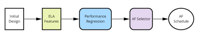
Refer to caption — Figure 1: How to select acquisition function (AF) schedules Based on the evaluated initial design of a BO run, we compute the ELA features. With those we query a trained RF and observe the predicted performance of each AF schedule. The Acquisition Function Selector returns the AF schedule with the best predicted performance to use for surrogate-based evaluations.

Motivated by recent insights from the AS domain, we aim to understand the interplay between the problem (characterized through the initial design), the choice of the AF (schedule), and the BO performance. To this end, we benchmark our approach on a test suite of well-established black-box numerical optimization problems, the BBOB functions of the COCO framework (Hansen et al., 2021). We build and train a model, called the Acquisition Function Selector (AFS) (Figure 1), which automatically selects the best suited AF (schedule) for a certain problem. To represent problems, we employ exploratory landscape analysis (ELA) (Mersmann et al., 2011). ELA is a framework for the extraction and computation of low-level numerical landscape features of black-box problems (related to e.g., multimodality, separability, conditioning, presence of plateaus, etc.) from sampled points and their evaluations. Here, we use the evaluated initial design for computing the ELA features. Since BO anyway evaluates the initial design before starting the surrogate-based optimization process, the use of ELA features comes at no evaluation cost. Our AF schedules are composed of either PI (more exploitative), EI (more explorative) or combinations of both.

Our key insights are that (i) already a selector built on top of a naïve random forest regression model outperforms any static AF schedule, (ii) the choice of the AF model should depend on the problem instance, but also on the characteristics (and in particular the quality) of the initial design, and (iii) the schedules that switch from EI to PI improve over static EI and PI.

2 Experiments

Building our Acquisition Function Selector (AFS) (see Figure 1) consists of two steps. First, we gather performance data of our seven AF schedules (static EI, static PI, and five dynamic ones: random, round robin, as well as three variants of explore-exploit schedules that switch from EI to PI after $25\text{\,}\mathrm{\char 37\relax}$ , $50\text{\,}\mathrm{\char 37\relax}$ and $75\text{\,}\mathrm{\char 37\relax}$ of the budget). Second, we train our AFS in the following way. We build a multi-target regression model that maps the ELA features of the initial design to the performance of each AF schedule. Our AFS then selects the schedule with the best predicted performance.
We evaluate our schedules on the $24$ single-objective noiseless BBOB functions of the COCO benchmark (Hansen et al., 2021) in dimension $5$ and $5$ instances with $60$ seeds). The size of the initial design is set to $10d=50$ data points and a budget of $40d=100$ function evaluations is used for the surrogate-based optimization part. The initial design is the same for every seed, so every schedule sees the same initial design. We adapt SMAC3 (Lindauer et al., 2022) to enable dynamic AF schedules and we use a Gaussian Process (GP) as surrogate model. We extract ELA features based on samples of the initial design and their function evaluations using the flacco library (Kerschke and Trautmann, 2019). Among the $300$ features (grouped in sets) in the library, we choose $38$ cheap-to-compute features not requiring further function evaluations, namely those from y-Distribution, Meta-Model, Dispersion, Information Content and Nearest-Better Clustering feature sets, following practices in the literature (Belkhir et al., 2016; Jankovic et al., 2021). In our setup, ELA feature computation for an initial design of $50$ points takes about $0.4\text{\,}\mathrm{s}$ , which is negligible compared to an expensive function evaluation. In this work, we restrict our attention to continuous problems, but ELA may also work well for discrete (and possibly mixed-integer) search spaces (Pikalov and Mironovich, 2022). We then train a standard random forest (RF) (Ho, 1995; Pedregosa et al., 2011) model ( $70/30$ train/test split) to regress the performance (log regret, normalized per problem) for each schedule based on the input ELA features. The schedule with the best predicted performance is selected by the AFS.
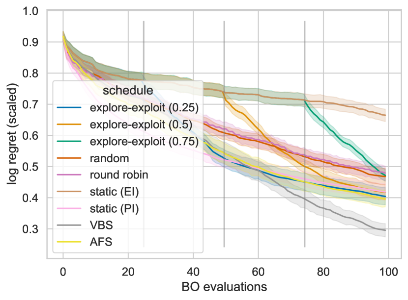
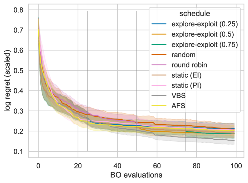
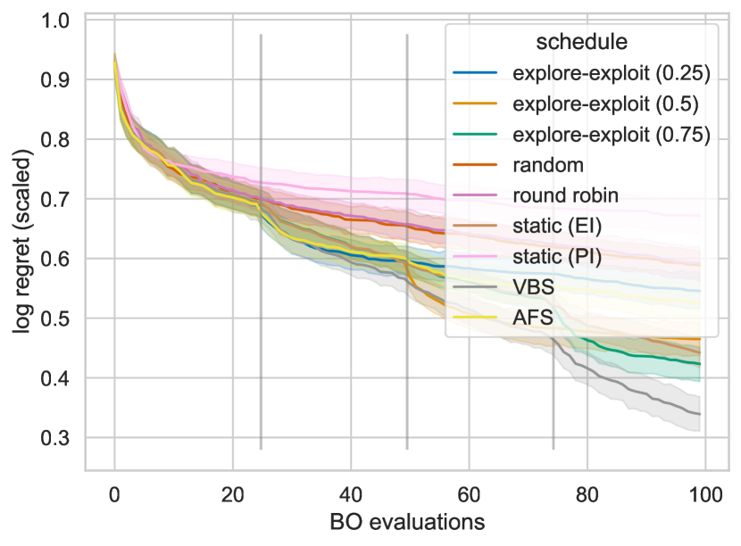
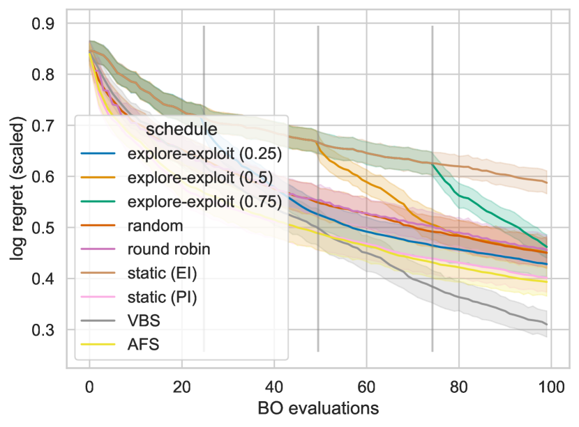
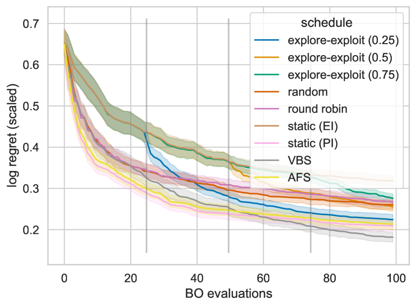
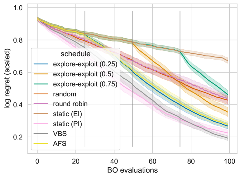
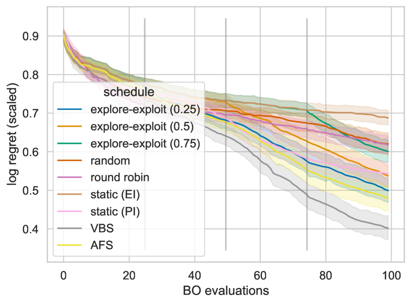
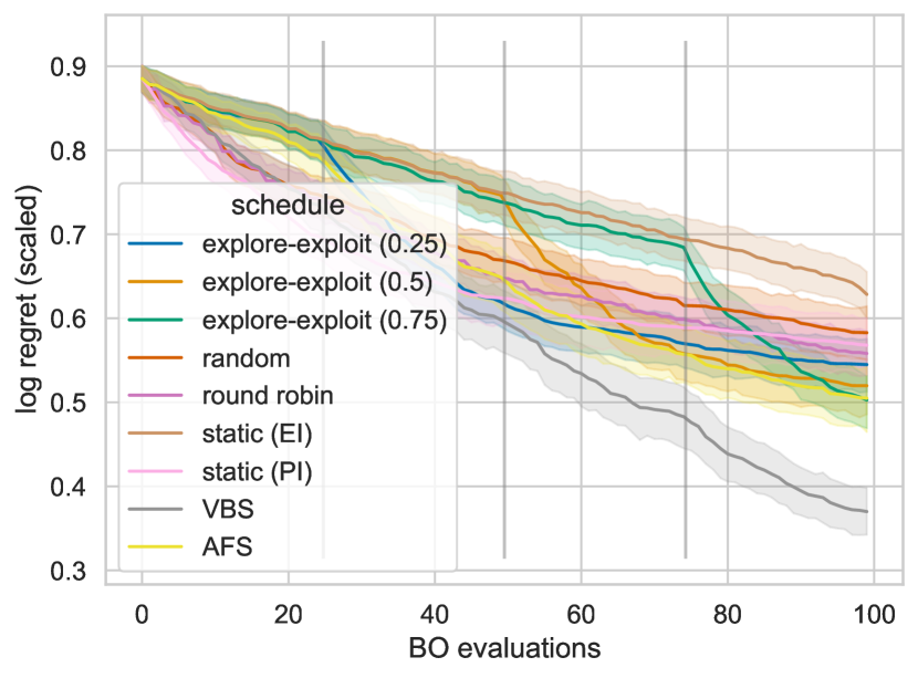
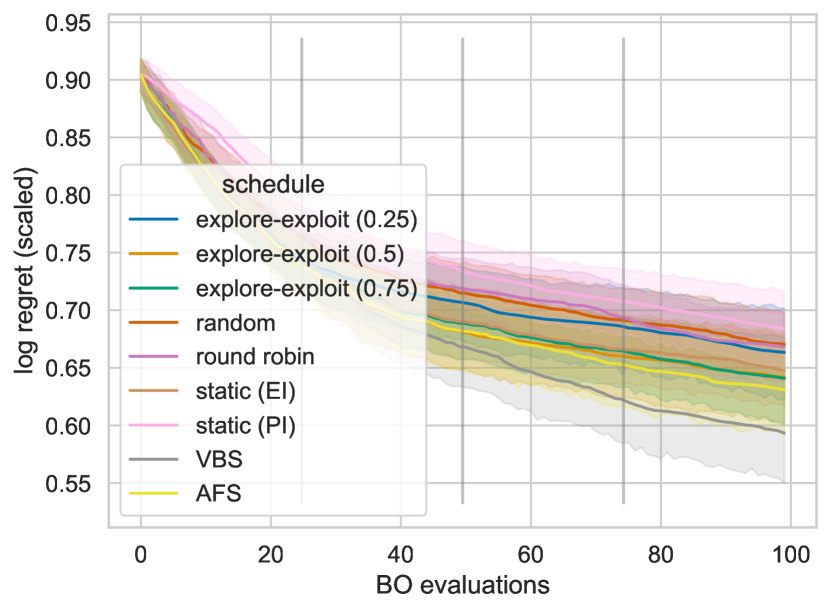
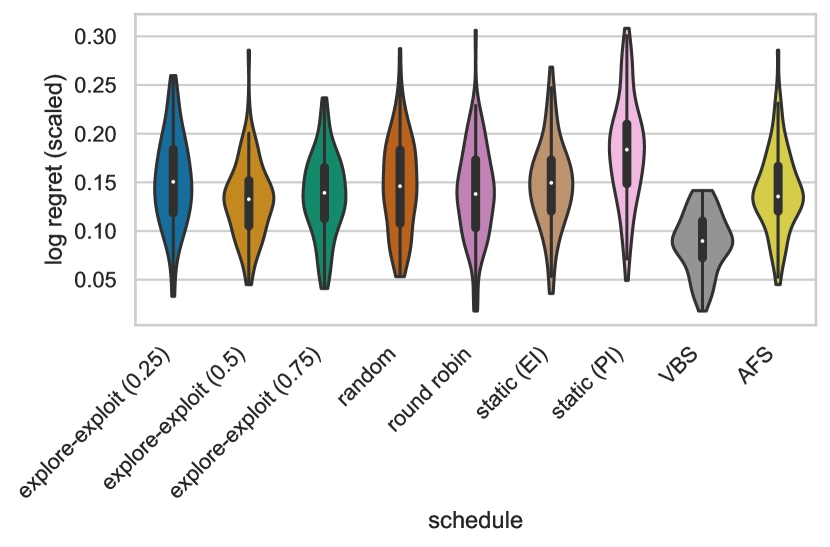
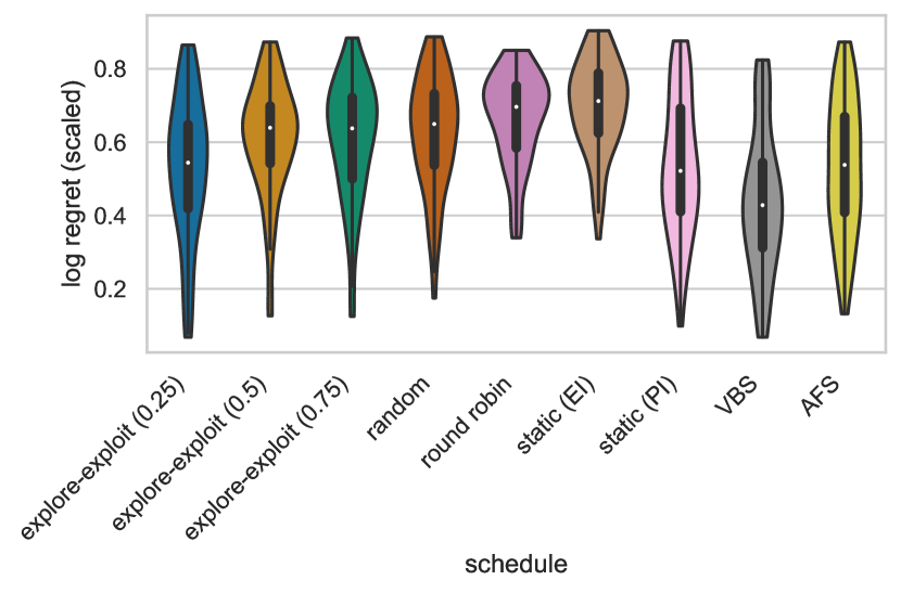
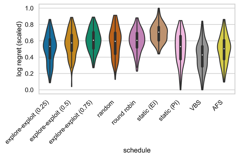
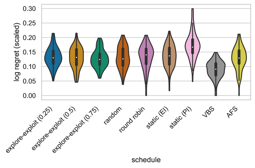
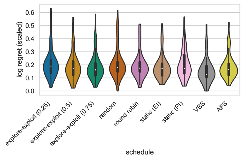
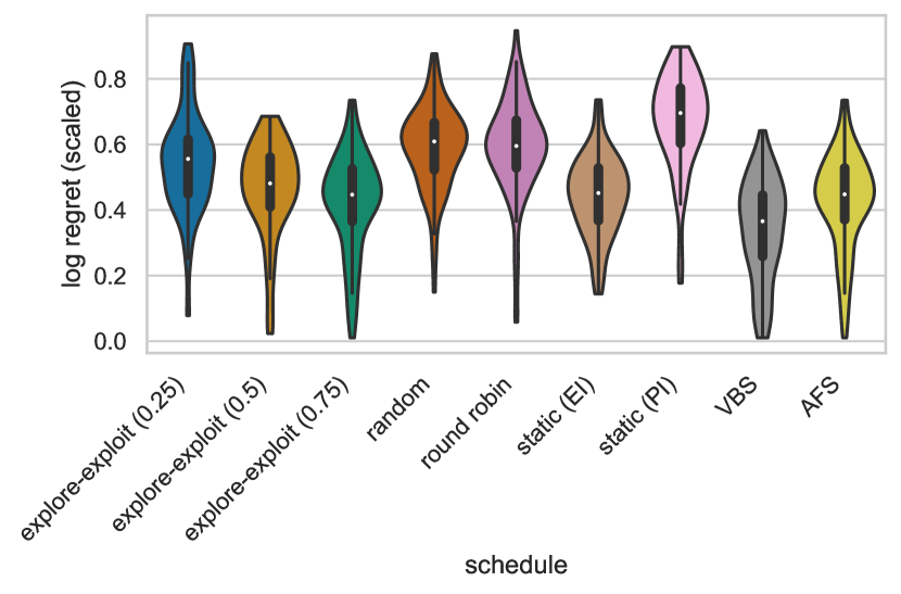
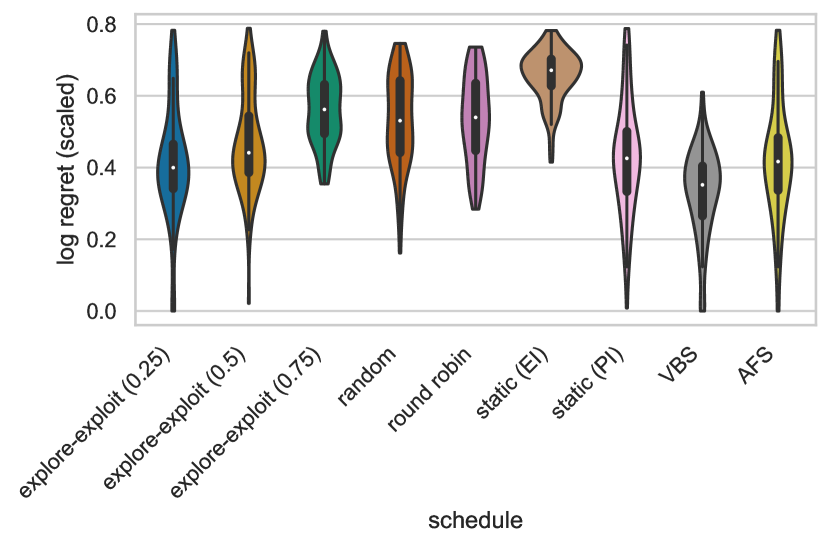
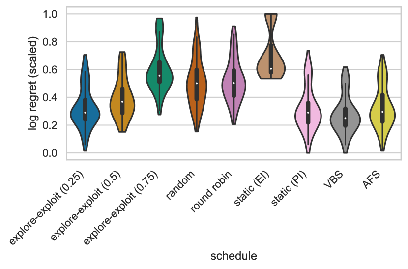
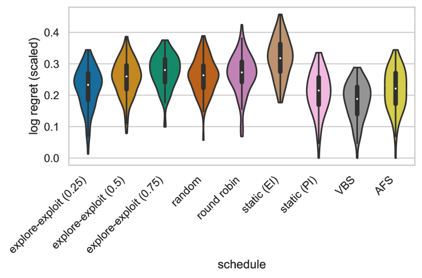
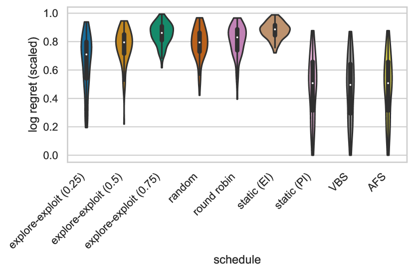
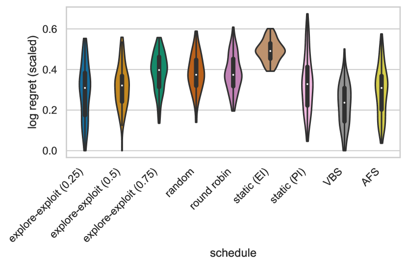
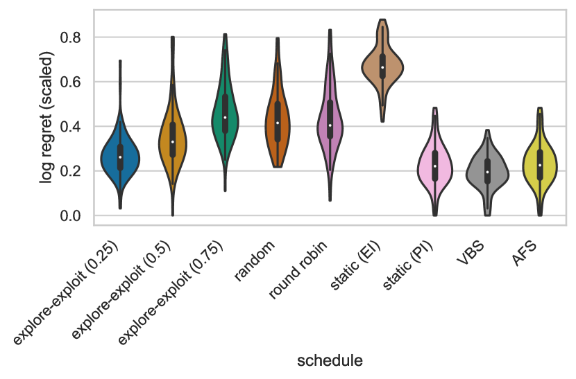
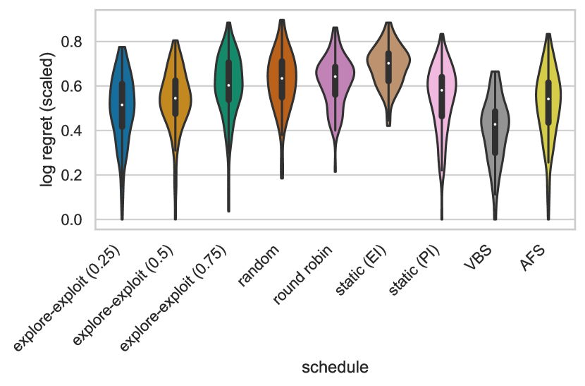
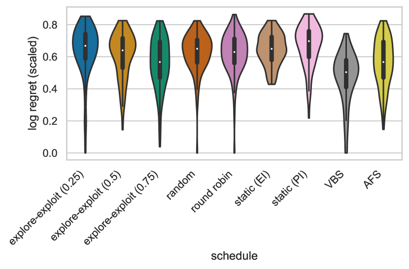
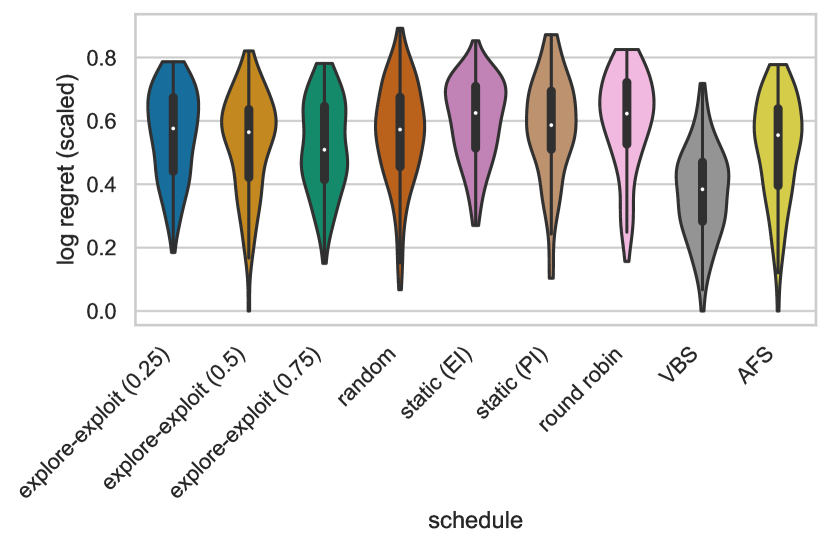
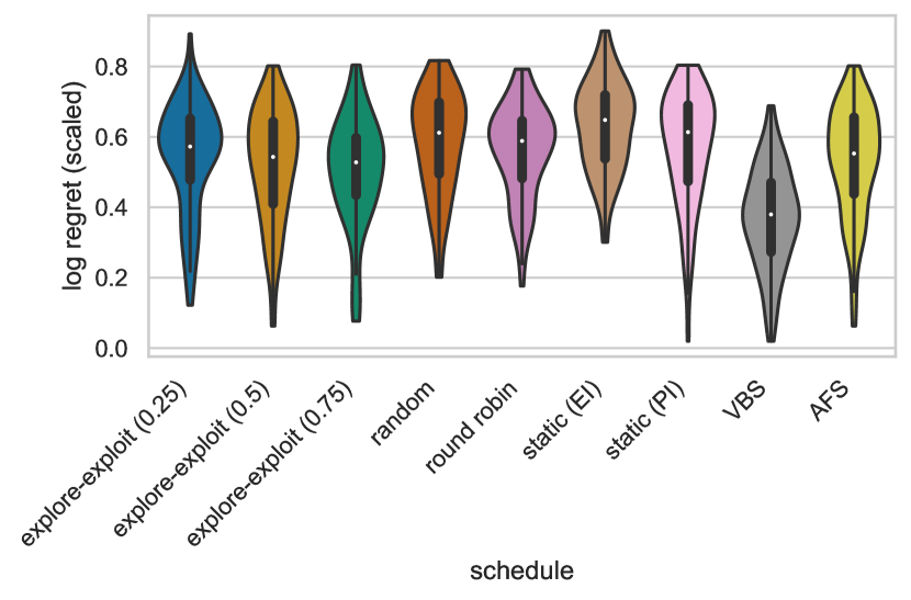
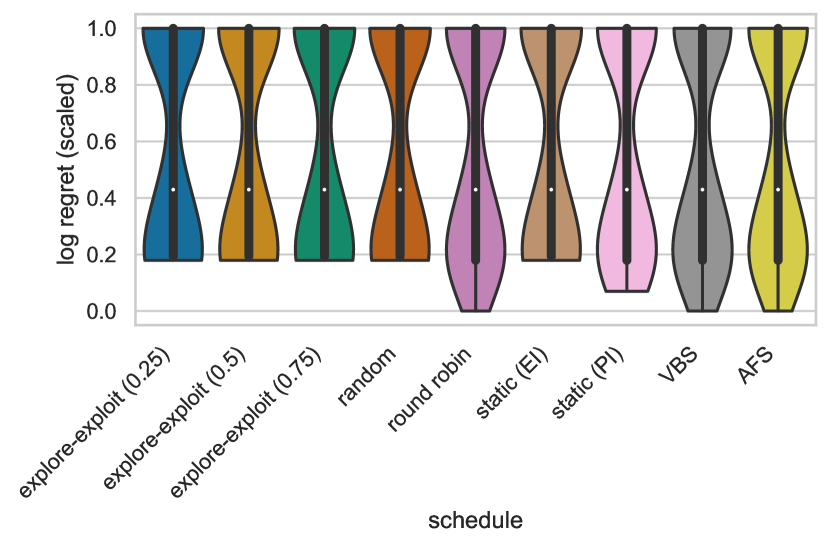
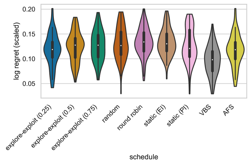
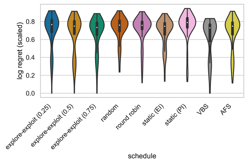
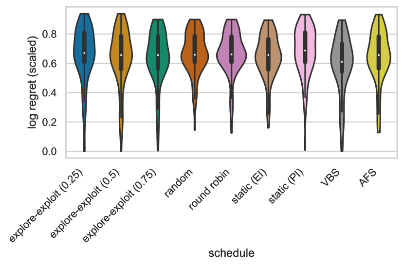
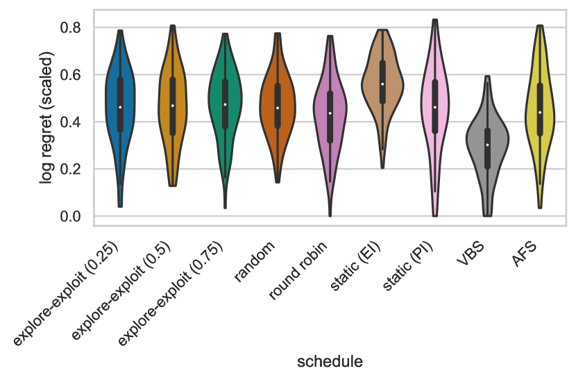
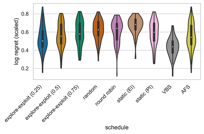
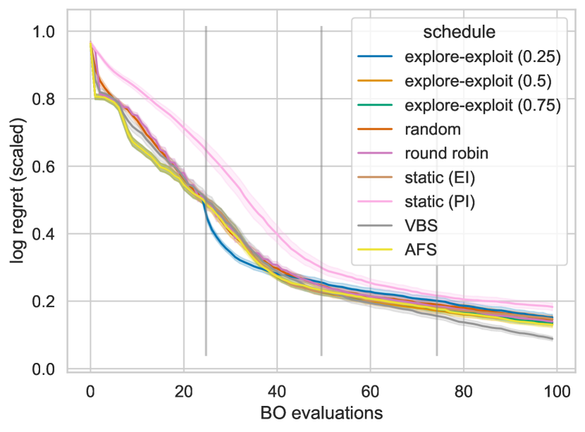
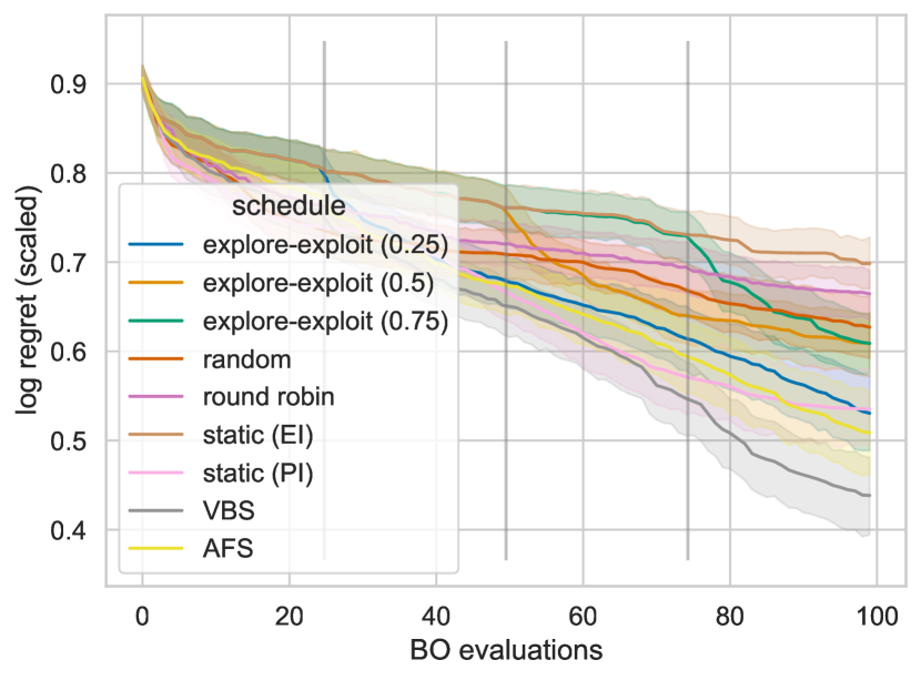
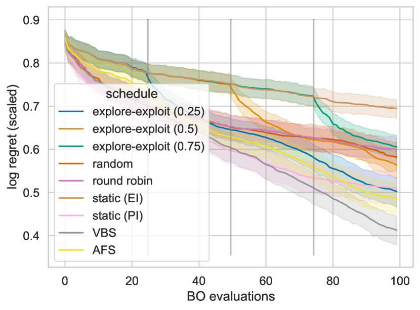
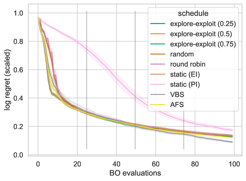
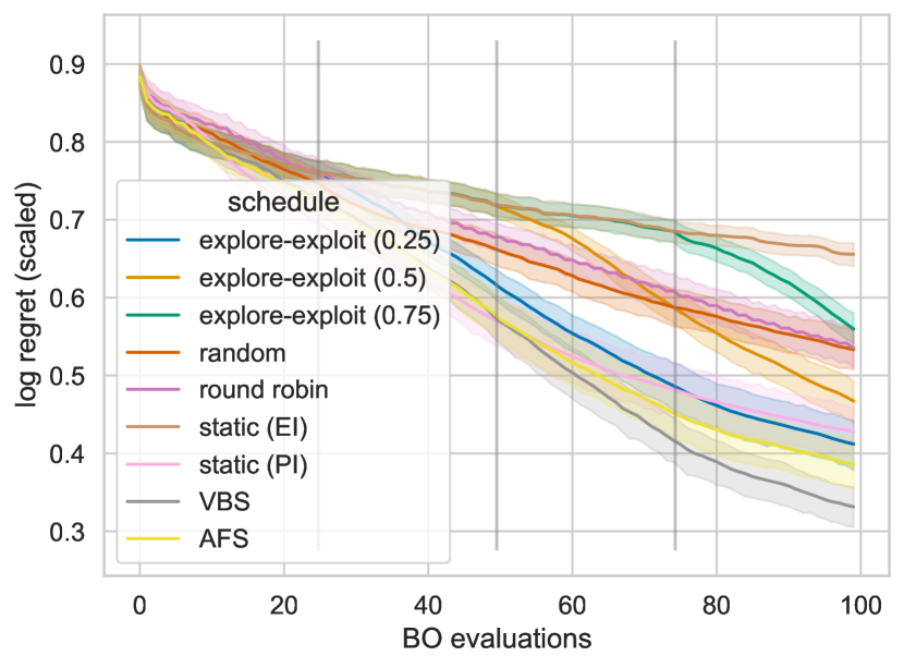
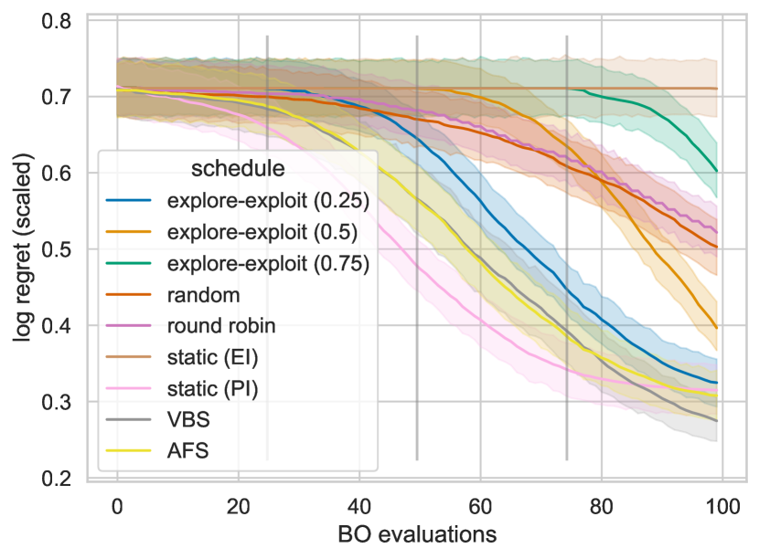
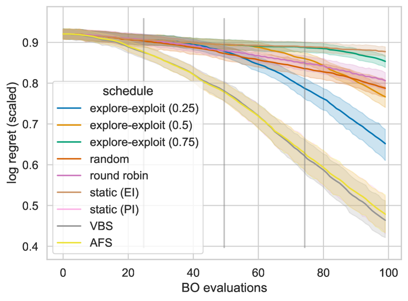
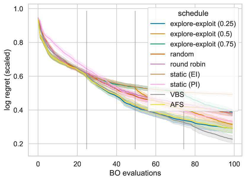
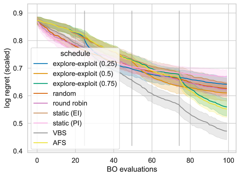
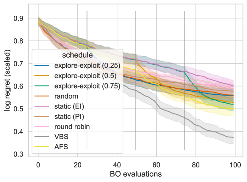
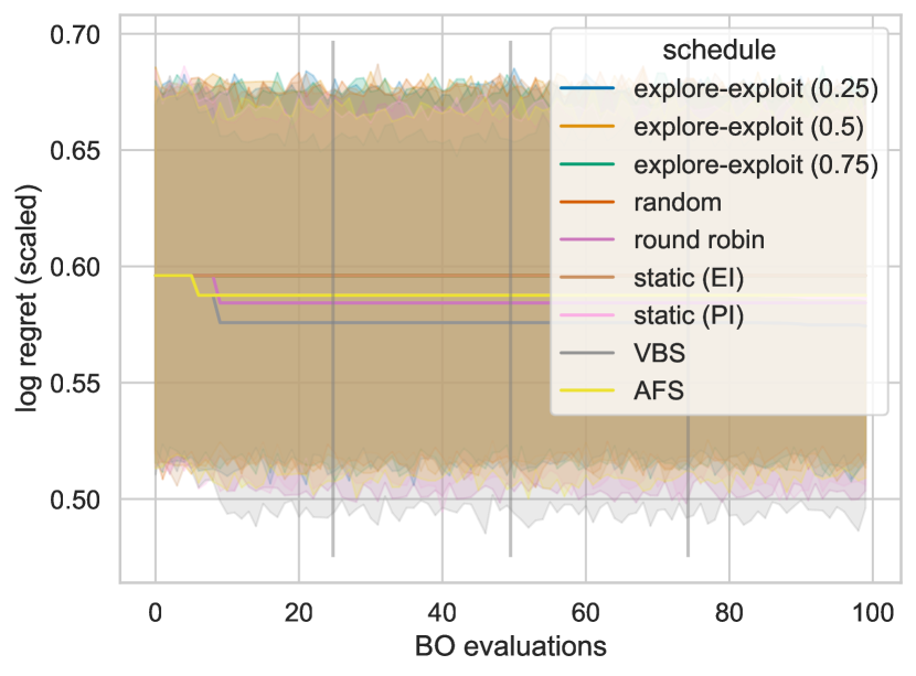
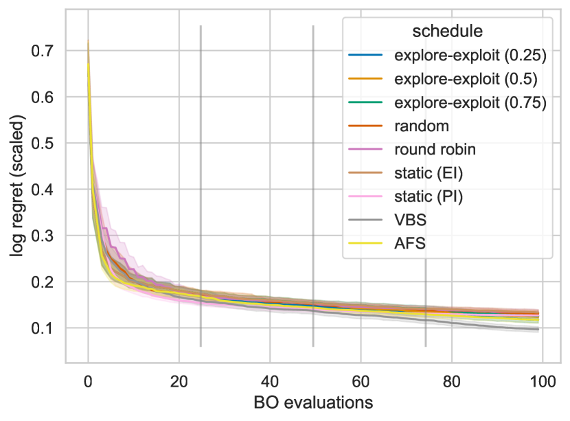
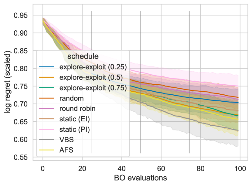
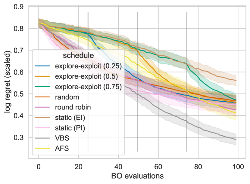
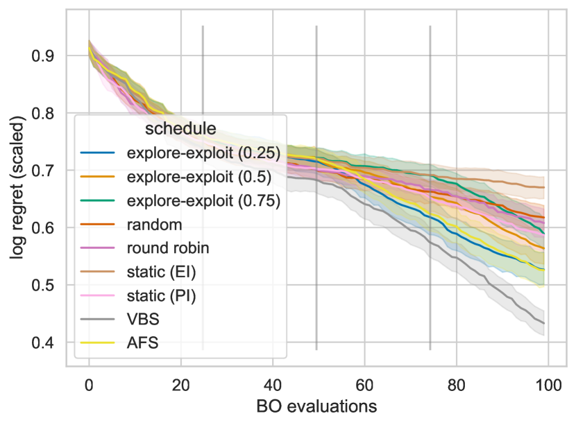
All experiments were conducted on a Slurm CPU cluster with $1592$ CPUs available across nodes. For visualization, we consider the log-regret of the incumbent (best evaluated search point) and only visualize the evaluations proposed by BO, omitting the initial design. In the violin plots, the log-regret of the final incumbents of all $60$ seeds are normalized to $[0,1]$ per BBOB function. In the convergence plots, the log-regret of the incumbents are normalized across runs to $[0,1]$ per BBOB function, and the means with the $95\text{\,}\mathrm{\char 37\relax}$ confidence intervals are shown. 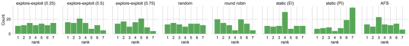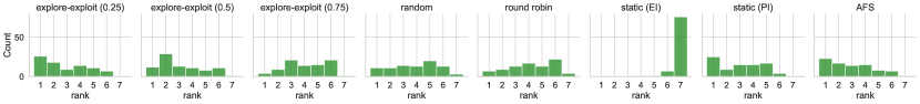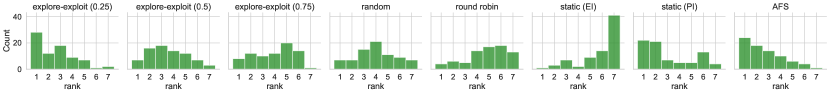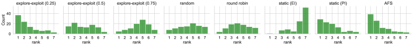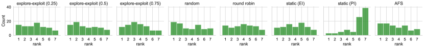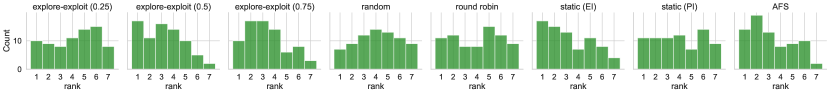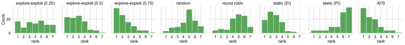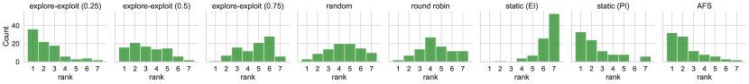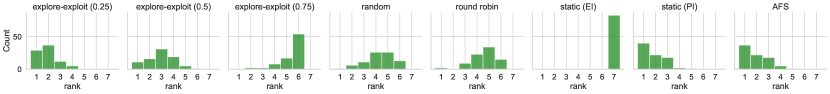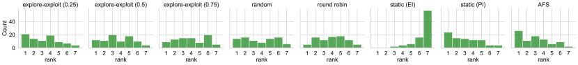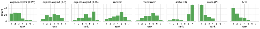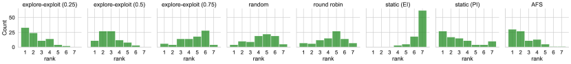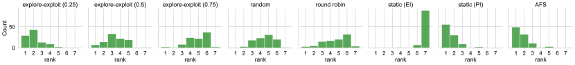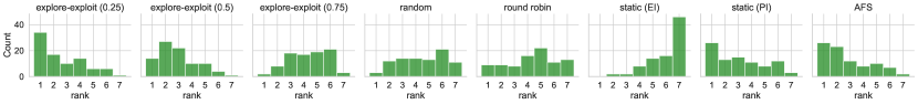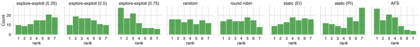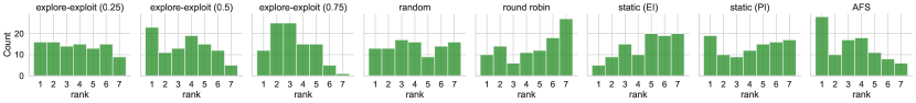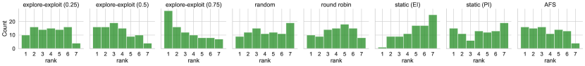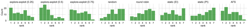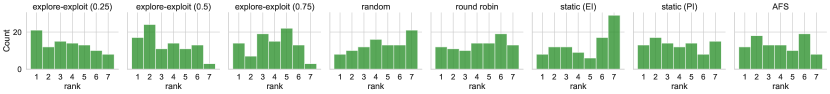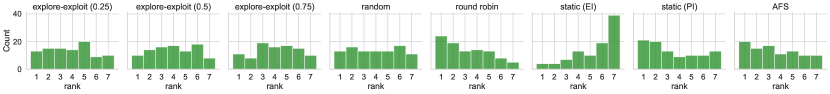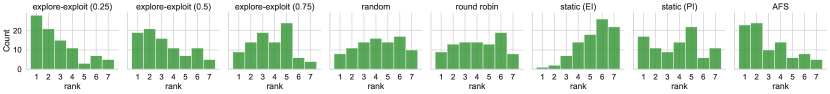Ranking is computed per run, i.e. per seed, BBOB function and instance. The AFS is assigned the same rank as the schedule it chose. We only plot performance on the test data. The plots for each function can be found in Appendix B. You can find the repository here: https://github.com/automl/BO-AFS.

Results

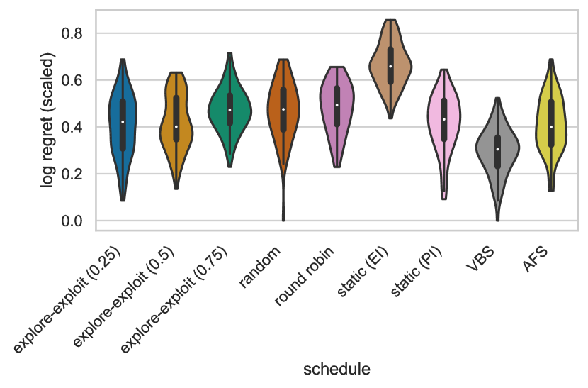
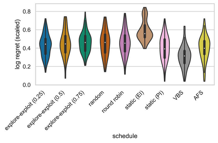
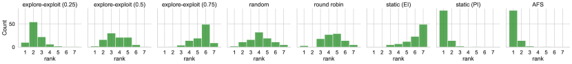
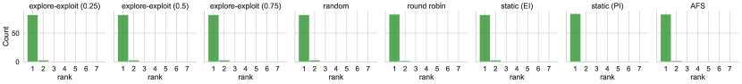
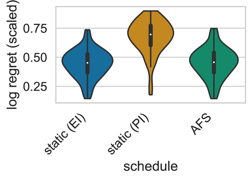
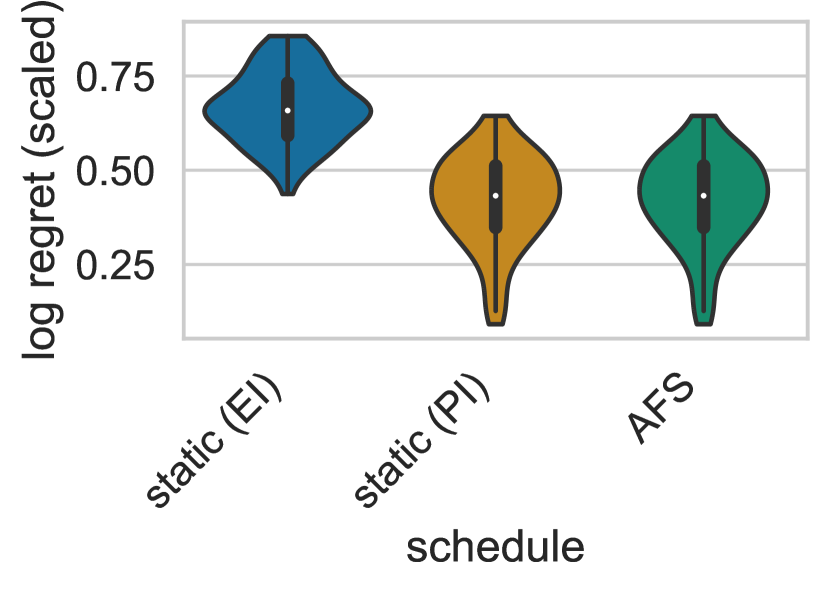
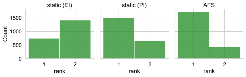
Before we learn to select from our portfolio containing static and dynamic schedules, we first consider selecting either static PI or static EI. We can observe that AFS adopts the shape of the better performing acquisition function (Figures 2(a) and 2(b)) and aggregated over all functions ranks first (Figure 2(c)), demonstrating the potential to select between AFs based on the initial design.

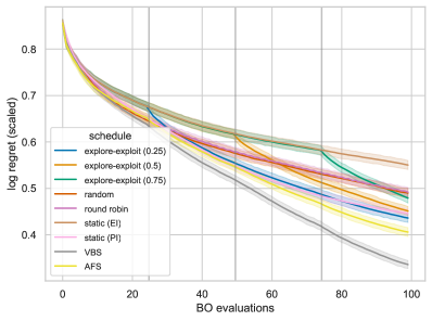
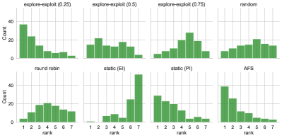
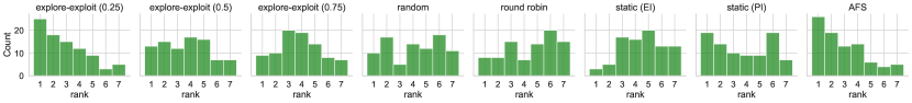
We then extend the AFS to select between all seven proposed schedules. We introduce the virtual best solver (VBS), which is our oracle, always selecting the best schedule per run. The general optimal choice of static or dynamic AF schedules depends on the problem at hand (see figures in Appendix B). As a rule of thumb, switching from EI to PI after a certain percentage of the budget of total number of function evaluations is beneficial and can boost performance, see Figure 4. However, the optimal switching point is highly problem-dependent and likely run-dependent. On average, switching after $25\text{\,}\mathrm{\char 37\relax}$ seems to be a viable general rule if the problem’s properties are unknown. Moreover, due to the initial design, we gain information about the problem landscape based on ELA features for that specific run. Already with a simple, non-tuned RF, we are able to select well-performing schedules with the AFS. In this case, the AFS (apart from the VBS) also shows the best anytime-performance which is not necessarily guaranteed as the AFS is trained on the final performance of the other schedules. Again, we rank across all functions and instances and observe that the mass of ranks for AFS is centered on the first, in contrast to all other schedules, see Figure 4. In summary, our AFS is able to propose appropriate schedules from a portfolio based on the initial design per run.

3 Conclusion and Future Work

Using a standard test bed for benchmarking single-objective numerical black-box optimization techniques, the BBOB suite of the COCO environment, we have shown in this work that a per-run selection of the acquisition function can benefit the performance of Bayesian optimization (BO) approaches. More precisely, we have seen that a landscape-aware selection of the AF, choosing from a portfolio of seven different AF schedules, outperforms any static choice. This advantage was realized with a naïve random forest regression approach, and it seems likely that further improvements can be expected from a proper model selection, e.g., using auto-sklearn (Feurer et al., 2020).
Our long-term objective is the development of modular BO algorithms that are trained to select their modules, including the AF, on the fly, i.e., during the optimization process. Such dynamic algorithm configuration (DAC) (Biedenkapp et al., 2020, 2022) approaches were recently shown capable of outperforming classic (static) hyperparameter optimization approaches. A key issue in the design of DAC is the identification of features that the trained model can use to guide its selection. Our results provide strong motivation to consider exploratory landscape analysis for this purpose. Blending the ELA features with information obtained from the surrogate model clearly is a natural next step for our work.
In our study, we have used a relatively large initial design size ( $10d$ points or $1/3$ of the total budget). Considering (Bossek et al., 2020), an intermediate decision whether to continue with the initial design or to start the surrogate-based optimization should bring additional performance gains. To realize this potential, a thorough investigation of suitable ELA features is needed, since some features cannot be considered reliable when based on such comparatively small sample sizes (Belkhir et al., 2016).
We see our work as a continuation of the per-run algorithm selection approach suggested in (Jankovic et al., 2022; Kostovska et al., 2022). In particular, we believe that it is not only the instance per se that should guide the selection of algorithm components and configurations, but also the particular trajectory that the algorithm follows in a particular run. In the future, we aim to develop a deeper understanding for when to switch from initial design sampling to using explorative AFs or exploitative ones. While in this first proof-of-concept study we have only considered EI and PI as AFs, in future studies we intend to include other AFs such as Upper Confidence Bound (UCB) (Forrester et al., 2008), Top-Two Expected Improvement (TTEI) (Qin et al., 2017), and Thompson Sampling (TS) (Thompson, 1933).

Acknowledgments

Our work has been financially supported by the the ANR T-ERC project VARIATION (ANR-22-ERCS-0003-01), by the CNRS INS2I project RandSearch, and by the PRIME programme of the German Academic Exchange Service (DAAD) with funds from the German Federal Ministry of Education and Research (BMBF), and by RFBR and CNRS, project number 20-51-15009. Carolin Benjamins and Marius Lindauer acknowledge funding by the German Research Foundation (DFG) under LI 2801/4-1.

References

Mockus (2012) Jonas Mockus. Bayesian Approach to Global Optimization: Theory and Applications. Springer Science & Business Media, December 2012. ISBN 978-94-009-0909-0.
Lindauer et al. (2019) M. Lindauer, M. Feurer, K. Eggensperger, A. Biedenkapp, and F. Hutter. Towards assessing the impact of bayesian optimization’s own hyperparameters. In IJCAI’19 DSO Workshop, 2019.
Cowen-Rivers et al. (2021) A. Cowen-Rivers, W. Lyu, R. Tutunov, Z. Wang, A. Grosnit, R. Griffiths, A. Maraval, H. Jianye, J. Wang, J. Peters, and H. Ammar. An empirical study of assumptions in Bayesian optimisation. arXiv:2012.03826 [cs.LG], 2021.
Bossek et al. (2020) Jakob Bossek, Carola Doerr, and Pascal Kerschke. Initial design strategies and their effects on sequential model-based optimization: an exploratory case study based on BBOB. In Proc. of Genetic and Evolutionary Computation Conference (GECCO’20), pages 778–786. ACM, 2020. doi: 10.1145/3377930.3390155. URL https://doi.org/10.1145/3377930.3390155.
Forrester et al. (2008) Alexander I. J. Forrester, András Sóbester, and Andy J. Keane. Engineering Design via Surrogate Modelling - A Practical Guide. John Wiley & Sons Ltd., 2008. ISBN 978-0-470-06068-1.
Thompson (1933) W. Thompson. On the likelihood that one unknown probability exceeds another in view of the evidence of two samples. Biometrika, 25(3/4):285–294, 1933.
Hoffman et al. (2011) Matthew Hoffman, Eric Brochu, and Nando de Freitas. Portfolio allocation for Bayesian optimization. In Proceedings of the Twenty-Seventh Conference on Uncertainty in Artificial Intelligence, UAI’11, pages 327–336, Arlington, Virginia, USA, 2011. AUAI Press. ISBN 9780974903972.
Kandasamy et al. (2020) Kirthevasan Kandasamy, Karun Raju Vysyaraju, Willie Neiswanger, Biswajit Paria, Christopher R Collins, Jeff Schneider, Barnabas Poczos, and Eric P Xing. Tuning hyperparameters without grad students: Scalable and robust Bayesian optimisation with dragonfly. J. Mach. Learn. Res., 21(81):1–27, 2020.
Rice (1976) J. Rice. The algorithm selection problem. Advances in Computers, 15:65–118, 1976.
Kerschke et al. (2019) Pascal Kerschke, Holger H. Hoos, Frank Neumann, and Heike Trautmann. Automated Algorithm Selection: Survey and Perspectives. Evolutionary Computation, 27(1):3–45, March 2019. ISSN 1063-6560. doi: 10.1162/evco_a_00242.
Jankovic et al. (2022) Anja Jankovic, Diederick Vermetten, Ana Kostovska, Jacob de Nobel, Tome Eftimov, and Carola Doerr. Trajectory-based algorithm selection with warm-starting. In IEEE Congress on Evolutionary Computation, CEC 2022, Padua, Italy, July 18-23, 2022, pages 1–8. IEEE, 2022. doi: 10.1109/CEC55065.2022.9870222. URL https://doi.org/10.1109/CEC55065.2022.9870222.
Kostovska et al. (2022) Ana Kostovska, Anja Jankovic, Diederick Vermetten, Jacob de Nobel, Hao Wang, Tome Eftimov, and Carola Doerr. Per-run algorithm selection with warm-starting using trajectory-based features. In Günter Rudolph, Anna V. Kononova, Hernán E. Aguirre, Pascal Kerschke, Gabriela Ochoa, and Tea Tusar, editors, Parallel Problem Solving from Nature - PPSN XVII - 17th International Conference, PPSN 2022, Dortmund, Germany, September 10-14, 2022, Proceedings, Part I, volume 13398 of Lecture Notes in Computer Science, pages 46–60. Springer, 2022. doi: 10.1007/978-3-031-14714-2\_4. URL https://doi.org/10.1007/978-3-031-14714-2_4.
Hansen et al. (2021) N. Hansen, A. Auger, R. Ros, O. Mersmann, T. Tušar, and D. Brockhoff. COCO: A platform for comparing continuous optimizers in a black-box setting. Optimization Methods and Software, 36:114–144, 2021. doi: 10.1080/10556788.2020.1808977.
Mersmann et al. (2011) Olaf Mersmann, Bernd Bischl, Heike Trautmann, Mike Preuss, Claus Weihs, and Günter Rudolph. Exploratory landscape analysis. In Natalio Krasnogor and Pier Luca Lanzi, editors, 13th Annual Genetic and Evolutionary Computation Conference, GECCO 2011, Proceedings, Dublin, Ireland, July 12-16, 2011, pages 829–836. ACM, 2011. doi: 10.1145/2001576.2001690. URL https://doi.org/10.1145/2001576.2001690.
Lindauer et al. (2022) M. Lindauer, K. Eggensperger, M. Feurer, A. Biedenkapp, D. Deng, C. Benjamins, T. Ruhkopf, R. Sass, and F. Hutter. SMAC3: A versatile bayesian optimization package for Hyperparameter Optimization. Journal of Machine Learning Research (JMLR) – MLOSS, 23(54):1–9, 2022.
Kerschke and Trautmann (2019) Pascal Kerschke and Heike Trautmann. Comprehensive feature-based landscape analysis of continuous and constrained optimization problems using the R-package FLACCO. In Nadja Bauer, Katja Ickstadt, Karsten Lübke, Gero Szepannek, Heike Trautmann, and Maurizio Vichi, editors, Applications in Statistical Computing – From Music Data Analysis to Industrial Quality Improvement, pages 93 – 123. Springer, 2019. doi: 10.1109/CEC.2016.7748359.
Belkhir et al. (2016) Nacim Belkhir, Johann Dréo, Pierre Savéant, and Marc Schoenauer. Surrogate assisted feature computation for continuous problems. In Proc. of Learning and Intelligent Optimization (LION’16), volume 10079 of LNCS, pages 17–31. Springer, 2016. doi: 10.1007/978-3-319-50349-3\_2. URL https://doi.org/10.1007/978-3-319-50349-3_2.
Jankovic et al. (2021) Anja Jankovic, Tome Eftimov, and Carola Doerr. Towards feature-based performance regression using trajectory data. In Pedro A. Castillo and Juan Luis Jiménez Laredo, editors, Applications of Evolutionary Computation - 24th International Conference, EvoApplications 2021, Held as Part of EvoStar 2021, Virtual Event, April 7-9, 2021, Proceedings, volume 12694 of Lecture Notes in Computer Science, pages 601–617. Springer, 2021. doi: 10.1007/978-3-030-72699-7\_38. URL https://doi.org/10.1007/978-3-030-72699-7_38.
Pikalov and Mironovich (2022) Maxim Pikalov and Vladimir Mironovich. Parameter tuning for the (1 + ( $\lambda$ , $\lambda$ )) genetic algorithm using landscape analysis and machine learning. In Juan Luis Jiménez Laredo, José Ignacio Hidalgo, and Kehinde O. Babaagba, editors, Applications of Evolutionary Computation - 25th European Conference, EvoApplications 2022, Held as Part of EvoStar 2022, Madrid, Spain, April 20-22, 2022, Proceedings, volume 13224 of Lecture Notes in Computer Science, pages 704–720. Springer, 2022. doi: 10.1007/978-3-031-02462-7\_44. URL https://doi.org/10.1007/978-3-031-02462-7_44.
Ho (1995) Tin Kam Ho. Random decision forests. In Proceedings of 3rd international conference on document analysis and recognition, volume 1, pages 278–282. IEEE, 1995.
Pedregosa et al. (2011) F. Pedregosa, G. Varoquaux, A. Gramfort, V. Michel, B. Thirion, O. Grisel, M. Blondel, P. Prettenhofer, R. Weiss, V. Dubourg, J. Vanderplas, A. Passos, D. Cournapeau, M. Brucher, M. Perrot, and E. Duchesnay. Scikit-learn: Machine learning in Python. 12:2825–2830, 2011.
Feurer et al. (2020) M. Feurer, K. Eggensperger, S. Falkner, M. Lindauer, and F. Hutter. Auto-sklearn 2.0: The next generation. arXiv:2007.04074[cs.LG], 2020.
Biedenkapp et al. (2020) A. Biedenkapp, H. F. Bozkurt, T. Eimer, F. Hutter, and M. Lindauer. Dynamic algorithm configuration: Foundation of a new meta-algorithmic framework. In Proc. of ECAI’20, pages 427–434, 2020.
Biedenkapp et al. (2022) A. Biedenkapp, N. Dang, M. S. Krejca, F. Hutter, and C. Doerr. Theory-inspired parameter control benchmarks for dynamic algorithm configuration. In Proc. of GECCO’22, 2022.
Qin et al. (2017) Chao Qin, Diego Klabjan, and Daniel Russo. Improving the Expected Improvement Algorithm. In Advances in Neural Information Processing Systems, volume 30. Curran Associates, Inc., 2017.

Checklist

1.
For all authors…
1. (a)
  
  Do the main claims made in the abstract and introduction accurately reflect the paper’s contributions and scope? [Yes]
2. (b)
  
  Did you describe the limitations of your work? [Yes]
3. (c)
  
  Did you discuss any potential negative societal impacts of your work? [No] We see no potential negative societal impact because our method is about speeding up an existing black-box optimization algorithm, therefore reducing required resources.
4. (d)
  
  Have you read the ethics review guidelines and ensured that your paper conforms to them? [Yes]
2.
If you are including theoretical results…
1. (a)
  
  Did you state the full set of assumptions of all theoretical results? [N/A]
2. (b)
  
  Did you include complete proofs of all theoretical results? [N/A]
3.
If you ran experiments…
1. (a)
  
  Did you include the code, data, and instructions needed to reproduce the main experimental results (either in the supplemental material or as a URL)? [Yes] https://github.com/automl/BO-AFS
2. (b)
  
  Did you specify all the training details (e.g., data splits, hyperparameters, how they were chosen)? [Yes]
3. (c)
  
  Did you report error bars (e.g., with respect to the random seed after running experiments multiple times)? [Yes]
4. (d)
  
  Did you include the total amount of compute and the type of resources used (e.g., type of GPUs, internal cluster, or cloud provider)? [Yes]
4.
If you are using existing assets (e.g., code, data, models) or curating/releasing new assets…
1. (a)
  
  If your work uses existing assets, did you cite the creators? [Yes]
2. (b)
  
  Did you mention the license of the assets? [N/A]
3. (c)
  
  Did you include any new assets either in the supplemental material or as a URL? [No]
4. (d)
  
  Did you discuss whether and how consent was obtained from people whose data you’re using/curating? [N/A] We create our own data.
5. (e)
  
  Did you discuss whether the data you are using/curating contains personally identifiable information or offensive content? [N/A]
5.
If you used crowdsourcing or conducted research with human subjects…
1. (a)
  
  Did you include the full text of instructions given to participants and screenshots, if applicable? [N/A]
2. (b)
  
  Did you describe any potential participant risks, with links to Institutional Review Board (IRB) approvals, if applicable? [N/A]
3. (c)
  
  Did you include the estimated hourly wage paid to participants and the total amount spent on participant compensation? [N/A]

Appendix A Acquisition Function Schedules

[Uncaptioned image] — Table 1: Schedule portfolio of PI, EI and their combinations. AFS is a selector that aims to predict which of the first seven schedules is the best. VBS is a perfect selector and forms the ground truth for AFS.

Name	Schedule
static (EI)
static (PI)
random
round robin
explore-exploit ( $0.25$ )
explore-exploit ( $0.5$ )
explore-exploit ( $0.75$ )
VBS (Virtual Best Solver)
AFS (AF Selector)

Appendix B Additional Results

In this section we provide all boxplot and convergence figures for each BBOB function. Please note that because the VBS is selected based on final performance, it does not always show the best anytime-performance.

We first present a more in-depth discussion of the results on specific BBOB functions, focusing on the manually defined schedules. A first observation is that switching from EI to PI is in general beneficial when the function landscape has an adequate global structure (F1-F19). Here, the only exceptions are F5 and F19. F5 is a purely linear function, where EI performs best as it explores fast in the beginning and exploits sufficiently fast later on because of the simplicity of the landscape. For F19, we hypothesize that only PI is able to exploit a lucky initial design landing close to optima.

In addition, we can see that PI works well for uni-modal and quite smooth functions (F1-F14), while performing even better when used after the switch. This observation is in line with PI’s exploitative behavior. In these cases exploiting does not miss any other optima further away in the landscape.

In contrast, PI is in general worse than EI and also not beneficial after the switch for multi-modal functions with weak global structure (F20-F24). Again, this is in line with our intuition because for these functions we have many important basins of attraction that have to be discovered before starting exploitation. The only exception is F23 (Figure 27), a rugged function with a high number of global optima, where the probability of starting in a basin of attraction is high and thus exploitation is a viable strategy. Also, the flatter the landscape the worse PI performs which can be also seen in F7 (slope with step, Figure 11).

Besides the static and the switching schedules, round robin switches from EI to PI and vice versa for each new function evaluation. The round robin schedule creates a step-wise progress, but is never the best strategy. Apparently, less frequent switching is preferable in order to take advantage of the strengths of each AF. On average, the random schedule performs similarly to round robin, but with a smoother progression. Most likely, the random schedule still switches too frequently for the AFs to work effectively.

On F16 we observe that a late switch from EI to PI performs best, see Figure 20(b). We can also nicely spot the general boosts after switching after $25\text{\,}\mathrm{\char 37\relax}$ , $50\text{\,}\mathrm{\char 37\relax}$ and $75\text{\,}\mathrm{\char 37\relax}$ . F16 has a highly rugged and moderately repetitive landscape with many local optima with evident quality difference. Therefore, PI can be trapped in a bad local optimum if applied too early.